Hyperspectral Target Detection Based on Masked Autoencoder Data Augmentation

Abstract

Deep metric learning combines deep learning with metric learning to explore the deep spectral space and distinguish between the target and background. Current target detection methods typically fail to accurately distinguish local differences between the target and background, leading to insufficient suppression of the pixels surrounding the target and poor detection performance. To solve this issue, a hyperspectral target detection method based on masked autoencoder data augmentation (HTD-DA) was proposed. HTD-DA includes a multi-scale spectral metric network based on a triplet network, which enhances the ability to learn local and global spectral variations using multi-scale feature extraction and feature fusion, thereby improving background suppression. To alleviate the lack of training data, a masked spectral data augmentation network was employed. It utilizes the entire hyperspectral image (HSI) training the network to learn spectral variability through mask-based reconstruction techniques and generate target samples based on the prior spectrum. Additionally, in search of more optimal spectral space, an Inter-class Difference Amplification Triplet (IDAT) Loss was introduced to enhance the separation between the target and background when finding the spectral space, by making full use of background and prior information. The experimental results demonstrated that the proposed model provides superior detection results.

1. Introduction

Hyperspectral imaging technology captures the reflectance of targets across hundreds of spectral bands, providing detailed spectral information that can be used to differentiate between different types of materials and different states of the same material. In hyperspectral image (HSI) processing, target detection is directly influenced by the application value of the HSI. It plays a crucial role in various fields, including agriculture [1,2] environmental monitoring [3], geological exploration [4,5], and military surveillance [6,7].

Hyperspectral image target detection (HTD) primarily identifies and locates the target of interest in hyperspectral images by using the prior spectrum of the target. Spectral information divergence (SID) [8] and spectral angle mapping [9] compute the matching degree between the HSI pixels and the prior spectrum. The higher the match degree, the more likely it is to be considered a target. Target detection is achieved by setting a decision threshold for these match degrees. These algorithms are simple to understand and implement. Some methods [10] assume that the background follows a specific distribution by using binary hypothesis testing and applying the generalized likelihood ratio test for target detection. Thus, these algorithms depend on hypothesis testing. Other researchers [11,12], recognizing that the actual background distribution is unknown and hypothesis testing may not be suitable for target detection, proposed a filter-based constrained energy minimization (CEM) method. It designs a filter that produces a binary output of one for the target and zero for the background as accurately as possible. Other scholars [13] proposed orthogonal subspace projection (OSP) based on signal decomposition, which treats the spectrum of each pixel as a combination of different signals. Thus, the target and background can be distinguished by decomposing each signal. The sparse representation method [14] reconstructs pixels in HSI using linear combinations of dictionary elements, followed by detection using the reconstructed pixels.

In recent years, deep learning methods have been widely applied for feature extraction, change detection, and semantic segmentation. Some researchers have employed models such as convolutional neural networks (CNNs), transformers, and autoencoders (AE) to explore the spatial–spectral features of hyperspectral data for target detection [15]. CNN uses a dual-stream network architecture to capture the spectral features, preserve the discriminative spectral information of pixels, and enhance the separability between the target and background. Although CNN has strong local feature extraction capabilities, it is difficult to capture long-range dependency relationships. Hence, transformers are used to enhance the ability to extract global features with long-range dependencies and capture contextual information effectively [16]. These models require labeled data and [17] introduce self-supervision to the HTD to explore spectral variations in the HSI and supplement prior information, enabling unsupervised target detection.

Some other scholars have combined deep learning with metric learning methods and constructed discriminative networks that measure the distance between the target and the background, aiming to identify a feature space that can distinguish the target from the background [18]. The Siamese network is able to learn the boundaries between the target and background, but it encounters difficulties when the target is very similar to the background, as it does not introduce additional constraints to ensure these subtle differences are captured correctly. Therefore, ref. [19] triplet networks are utilized to determine the optimal feature space for HTD. The triplet network can distinguish similar targets and backgrounds in more detail because it not only requires the distance between pairs of positive samples to be small but also emphasizes that negative samples should be far enough away from positive samples to increase the ability to learn fine-grained features.

Owing to the spectral variability and spectral mixing in HSI, the spectrum of the target sample and three background samples show similar trends and minor inter-class differences, as shown in Figure 1. Ignoring the minor local differences between the target and background results in insufficient suppression around the target and reduced detection accuracy. To address this issue, we employed a multi-scale spectral metric network. Through multi-scale feature extraction and feature fusion, the ability to recognize subtle differences and suppress the background improves target detection accuracy.

Training the triplet network for HTD requires a large amount of triplet data consisting of target, prior spectrum, and background. Therefore, a data augmentation network is required to generate targets and backgrounds. There are three types of methods for data augmentation in HTD:

• Coarse detection-based;
• Synthesis-based;
• Mask-based methods.

Coarse detection-based methods [20] were first detected using a fast HTD method, where the pixels with the highest and lowest probabilities in the detection map were treated as the target and background, respectively. The obtained target samples were mixed with the background samples, affecting the detection results because the target only accounted for a small portion of the HSI.

Synthesis-based methods [15,19,21] combine the prior spectrum with the HSI at a specific ratio to generate target samples. The method is simple and small computationally. However, this ratio typically requires manual adjustment, resulting in inconsistent detection results.

Generative-based methods [22,23,24] utilize generative adversarial networks to generate realistic sample curves by learning the spectral variability of an image with a large number of parameters. Gao et al. [25] use generative adversarial networks to generate simulated target sample points and background sample points for sample enhancement. Compared to synthesis-based methods, generative methods are closer to the real spectrum and can cover a wide range of different scenes and conditions. However, they require careful design of generators and discriminators. A lot of parameter tuning is needed, and when there are few samples, they are also prone to overfitting.

We propose a masked autoencoder (MAE)-based spectral mask data augmentation network inspired by the MAE [26] that can automatically learn spectral variability and realize unsupervised data augmentation to generate a realistic target, requiring the adjustment of only a single parameter. The contributions of this study are as follows:

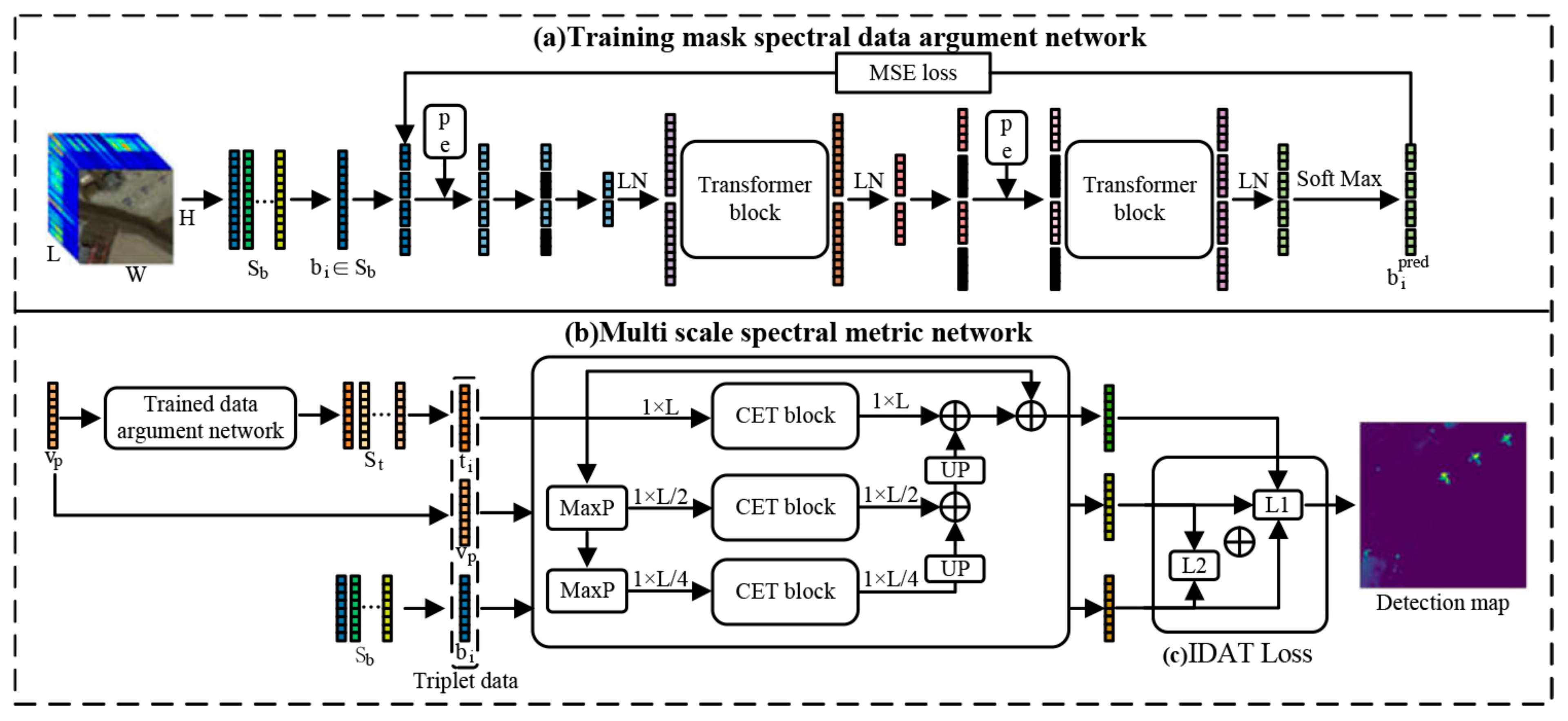
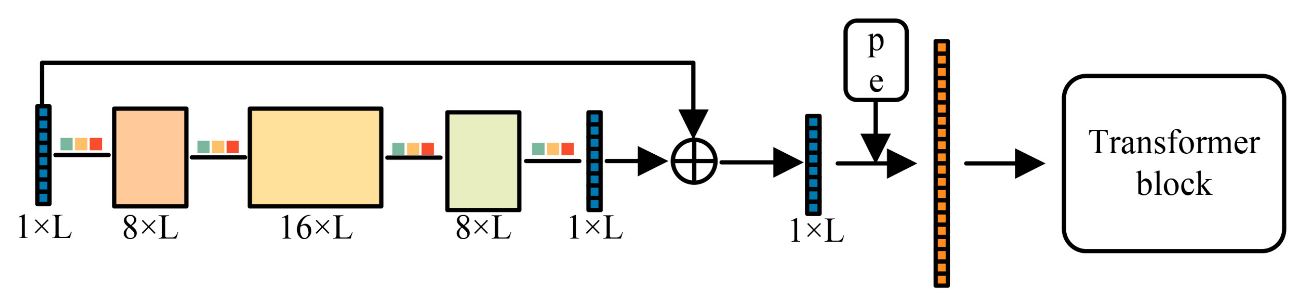
• A multi-scale spectral metric network is proposed; firstly, multi-scale feature vector construction is performed and a Convolutional Embedding Transformer (CET) block is proposed to extract local and global features of the feature vector and finally, the feature extraction results of multi-scale feature vector are fused to improve the ability to extract fine-grained features;
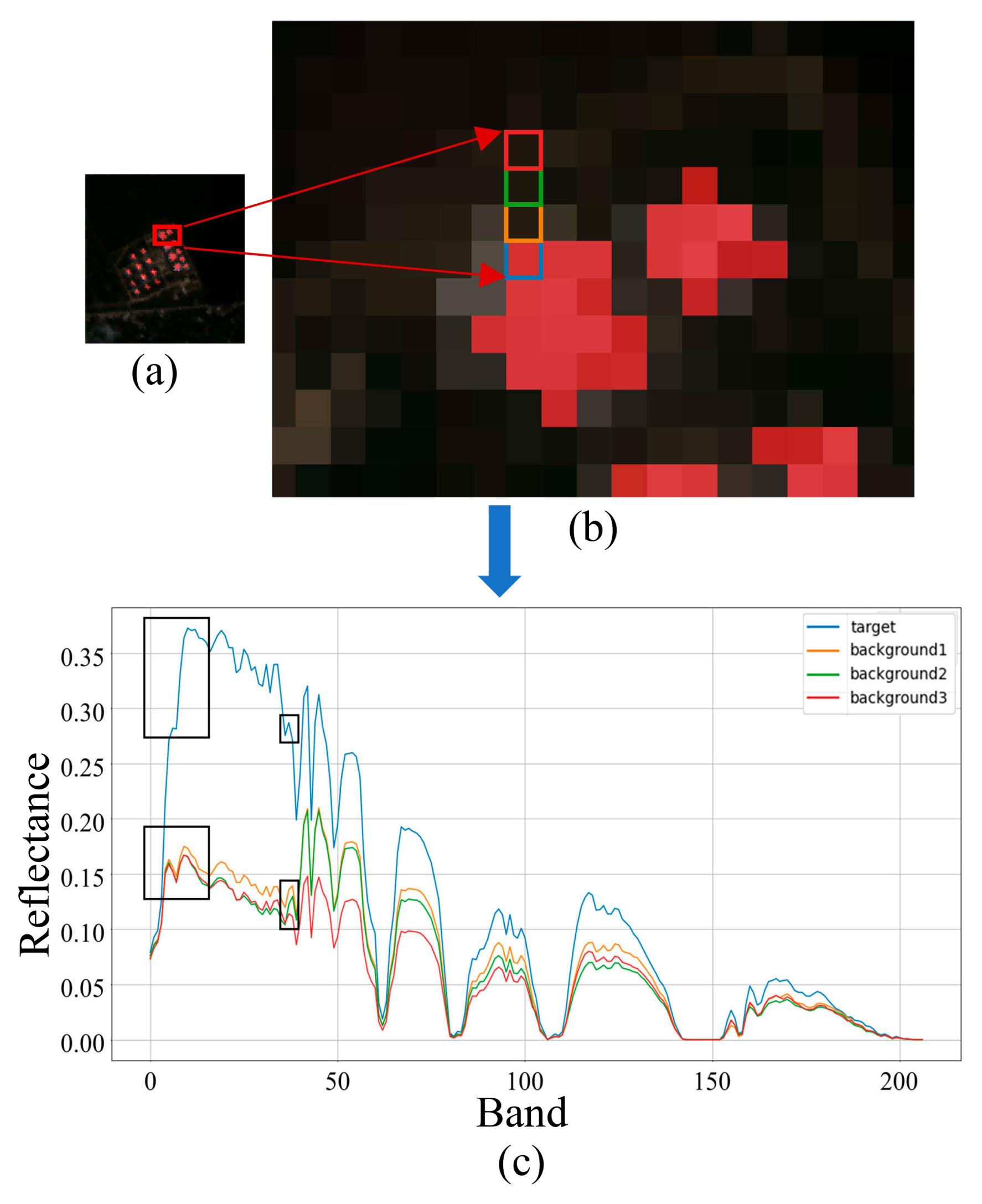
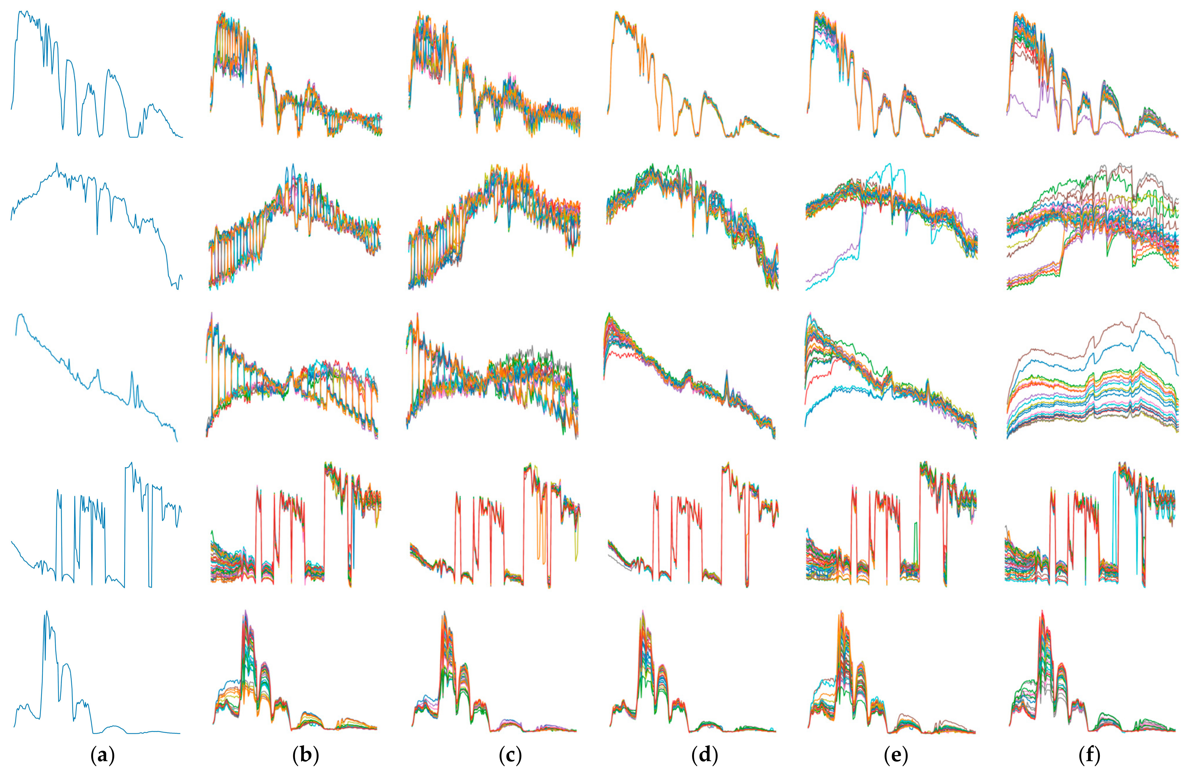
• A masked spectral data augmentation network was proposed to generate the target. The network learns spectral variability by dividing and masking the spectrum in the HSI, followed by reconstructing the spectrum. The prior spectrum is divided and masked to generate the target. The network is simple and requires adjustment of only the mask ratio to automatically learn the spectral variability for generating the target;
• Inter-class Difference Amplification Triplet Loss is proposed, based on the traditional triplet loss, to take into account the distance between the background and priori spectrum. The background information is fully utilized to enhance the discrimination between target and background.

2. Materials and Methods

2.1. Materials

2.1.1. Deep Metric Learning

The deep metric learning network is designed to identify a metric space that clusters same-class and separates different-class components. It includes a Siamese network and a triplet network, which can be used to differentiate between the target and background.

The Siamese network uses prior spectrum and HSI pixels as inputs and determines whether the pixel corresponds to the target [27,28]. Although Siamese Net performs well in two-by-two comparisons, it is essentially a binary classifier that can only determine whether two samples are similar. When multiple backgrounds are involved, additional designs are required to meet the requirements of complex tasks.

Therefore, triplet networks are gradually being applied to HTD. For a set of triplet data, including a target sample, prior spectrum, and background sample, the triplet network tries to learn a feature space in which the target and prior spectrum are close and the background is far away from the prior spectrum [19]. The triplet network groups spectral vectors for liner projection and adds hop-layer connections in the transformer block. Despite using deep residual convolution, the network is limited in its ability to extract features from high-dimensional spectral data, affecting the effectiveness of learning for small differences.

HSI usually contains a large amount of band information, and it is a challenge to efficiently extract key features from them that can help distinguish the target from the background. We design a multi-scale spectral metric network, which is able to perform local and global feature extraction and fuse multi-scale features to enhance the ability to capture long-range dependencies and global features.

2.1.2. Mask-Based Data Enhancement

Mask-based methods are inspired by the cutout method, which masks the prior spectrum to obtain the target [29]. It randomly masks the prior spectrum with zero to construct the target. Small clusters are discarded during the clustering process to obtain background using the density-based spatial clustering of applications with a noise clustering algorithm [30]. It employs a dropout strategy to drop the prior spectrum to generate a target and consider all pixels of the HSI as background. Owing to the strong redundancy in the spectral dimension, masking some bands retains part of the spectral information but reduces the ability to distinguish the background around the target, leading to poor background suppression.

In order to obtain more realistic targets, inspired by MAE, we designed a masked spectral data augmentation network. HSI pixels are masked and fed into the encoder and decoder to reconstruct and train the network to learn spectral variability. The prior spectrum is masked and input to the trained network to obtain the target.

2.1.3. MAE Network

As shown in Figure 2, MAE is a self-supervised learning method for computer vision that is widely used in the fields of image segmentation [31,32] and target detection [33]. MAE divides the image into patches, randomly masks some of the patches, and inputs them into an encoder–decoder to reconstruct masked patches. During the reconstruction, the network automatically learns image features and restores as much of the image as possible.

The encoder only encodes unmasked patches and the decoder uses the output of the encoder and the masked patches as input and reconstructs the image. The encoder and decoder are based on a vision transformer, utilizing patch embedding, linear projection, position embedding, and a transformer block.

Position encoding in MAE captures two-dimensional (2D) positional relationships around a patch, which is not suitable for processing spectral data. Therefore, in the masked spectral data augmentation network, we used one-dimensional (1D) position embedding to generate position information of the patch, generating more accurate targets.

2.2. Methods

A flowchart of the proposed method is shown in Figure 3. The algorithm can be divided into three main parts, which are as follows: masked spectral data augmentation network, multi-scale spectral metric network, and inter-class difference amplification triplet loss.

2.2.1. Masked Spectral Data Augmentation Network

Spectral variability exists in HSI. We used a background set in HSI to train the masked spectral data augmentation network; the network learns how to generate richer and more representative feature representations based on the input data. Once the network is fully trained, it can capture the spectral variability of HSI. Randomly masking the prior spectrum and inputting them into the trained network can generate more realistic target spectrums based on the variability features learned by the network.

According to the principle of suppressing background, all pixels of the $HSI\in R^{H\ast W\ast L}$ (H, W, and L denote the height, width, and number of channels of the image, respectively) are used as the background set $S_b={[b_1,b_2,b_3,...,b_N]}^T\in R^{N\ast L}$ ($b_i\in R^{L\ast 1},N=H\ast W$) to train the network.

Divide the background $b_i={\left[x_1,x_2,\dots ,x_L\right]}^T$ into non-overlapping Q patches, ${\left[p_1,p_2,\dots ,p_Q\right]}^T$ ($p_i\in R^{L/Q\ast 1}$). Put patch $p_i(i=\mathrm{1,2},3,...,Q$) into linear projection to obtain the potential representation $p_i^{\prime }\in R^{D\ast 1}$, which is represented by (1) and (2).

$${[p_1,p_2,\dots ,p_Q]}^T=divide\_into\_patch\left(b_i\right)$$

(1)

$${[p_1^{\prime },p_2^{\prime },\dots ,p_Q^{\prime }]}^T=LN\left({[p_1,p_2,\dots ,p_Q]}^T\right)$$

(2)

where $divide\_into\_patch\left(\right)$ denotes dividing into patches and LN denotes linear projection. Unlike MAE, only position encoding is performed because image classification is not required. Position embedding $pe$ uses 1D embedding instead of 2D embedding, which is more suitable for spectral data. By adding the 1D position embedding $pe$ with the patch, we obtain the embedded patch ${[{\mathrm{p}}_1^{\mathrm{e}},{\mathrm{p}}_2^{\mathrm{e}},{\mathrm{p}}_3^{\mathrm{e}},...,{\mathrm{p}}_{\mathrm{Q}}^{\mathrm{e}}]}^{\mathrm{T}}$. This is expressed by (3).

$${\left[p_1^e,p_2^e,p_3^e,\dots ,p_Q^e\right]}^T={\left[p_1^{\prime }\left|pe,p_2^{\prime }\right|pe,\dots ,p_Q^{\prime }|pe\right]}^T$$

(3)

$$pe={[{pe}_{(pos,2i)},{pe}_{(pos,2i+1)}]}^T(i=\mathrm{0,1},2,\dots ,Q/2)$$

(4)

$${pe}_{(pos,2i)}=sin(pos/{\mathrm{10,000}}^{2i/D})$$

(5)

$${pe}_{(pos,2i+1)}=cos(pos/{\mathrm{10,000}}^{2i/D})$$

(6)

where $i$ denotes patch index, ${pe}_{(pos,2i)}$ and ${pe}_{(pos,2i+1)}$ denote the embedding vectors of the even and odd positions, respectively, and $pos$ denotes the position of patch. Shuffling ${[p_1^e,p_2^e,p_3^e,...,p_Q^e]}^T$ randomly to disrupt the order of patches, like [$p_{\mathrm{Q}-1}^e,p_3^e,p_{\mathrm{Q}}^e,...,p_1^e$]. $P_{unmask}$ consists of the top 25% of patches and $P_{masked}$ consists of the last 75%. $P_{masked}$ is not input to the first transformer block; therefore, it realizes the masking. Inputting $P_{unmask}$ into the first conventional transformer block yields a latent representation $P_{unmasked}^{\prime }=[c_1,c_2,\dots ,c_Q]$($c_i\in R^{D\ast 1}$). This is expressed as (7)–(9).

$$P_{unmask}={top}_{25\mathrm{\%}}\left(\mathrm{S}\mathrm{h}\mathrm{u}\mathrm{f}\mathrm{f}\mathrm{l}\mathrm{e}\left({[p_1^e,p_2^e,p_3^e,...,p_Q^e]}^T\right)\right)$$

(7)

$$P_{masked}={bot}_{75\mathrm{\%}}\left(\mathrm{S}\mathrm{h}\mathrm{u}\mathrm{f}\mathrm{f}\mathrm{l}\mathrm{e}\left({[p_1^e,p_2^e,p_3^e,...,p_Q^e]}^T\right)\right)$$

(8)

$$P_{unmasked}^{\prime }={[c_1,c_2,\dots ,c_{Q/4}]}^T=Tb\left(P_{unmask}\right)$$

(9)

where $\mathrm{S}\mathrm{h}\mathrm{u}\mathrm{f}\mathrm{f}\mathrm{l}\mathrm{e}\left(\right)$ denotes a random shuffle, ${top}_{25\mathrm{\%}}$ denotes the top 25% of patches, and ${bot}_{75\mathrm{\%}}$ denotes the last 75% of patches. Tb denotes the transformer block. A linear projection of $P_{unmasked}^{\prime }$ obtains ${[c_1^{\prime },c_2^{\prime },\dots ,c_{Q/4}^{\prime }]}^T$($c_i^{\prime }\in R^{D/2\ast 1}$), has the learnable mask vector added $P_{masked}^{\prime }={[l_1,l_2,...,l_{3Q/4}]}^T$($l_i\in R^{D/2\ast 1}$), and is unshuffled, so that $P_{masked}^{\prime }$ learns the information of $P_{masked}$. By adding the position embedding pe and input to the transformer block, the $b_i^{\prime }$ is obtained, which learns the spectral information. However, the patch dimension $b_i^{\prime }$ is $R^{D/2\ast 1}$, so it needs to be projected onto $R^{L/Q\ast 1}$ for reconstruction, which is expressed by (10)–(12).

$$P_{unmasked}^{\prime \prime }={\left[c_1^{\prime },c_2^{\prime },\dots ,c_{Q/4}^{\prime }\right]}^T=LN\left({\left[c_1,c_2,\dots ,c_{{\displaystyle \frac{Q}{4}}}\right]}^T\right)$$

(10)

$$b_i^{\prime }=\mathrm{T}\mathrm{b}\left(\mathrm{p}\mathrm{e}+Unshuffle\left(\left[P_{unmasked}^{\prime \prime },P_{masked}^{\prime }\right]\right)\right)$$

(11)

$$b_i^{pred}=\mathrm{S}\mathrm{o}\mathrm{f}\mathrm{t}\mathrm{M}\mathrm{a}\mathrm{x}\left(\mathrm{L}\mathrm{N}\left(b_i^{\prime }\right)\right)$$

(12)

where $Unshuffle$() is used to restore the shuffle operation. $b_i^{pred}$ is the reconstructed $b_i$ containing $P_{unmask}$ and reconstructed $P_{masked}^{\prime }$, and the mean squared error (MSE) is used to calculate the loss between $P_{masked}^{\prime }$ and $P_{masked}$, as shown below by (13).

$$L_{MSE}={\left|\right|P_{masked}-P_{masked}^{\prime }\left|\right|}_2$$

(13)

where $L_{MSE}$ denotes the MSE loss. Using the background set trained network, the prior spectrum ${\mathrm{v}}_p\in R^{L\ast 1}$ is randomly masked using the same mask methods and fed into the trained network, which is repeated N times to obtain the target set $S_t=[t_1,t_2,t_3,...,t_N]$. The triplet dataset ${\mathrm{S}}_n=\left[\right\{t_1,{\mathrm{v}}_p,b_1\},\{t_2,{\mathrm{v}}_p,b_2\},...,\{t_N,{\mathrm{v}}_p,b_N\left\}\right]$ was combined with ${\mathrm{S}}_t$, ${\mathrm{v}}_p$, and ${\mathrm{S}}_b$. This network does not require parameter tuning; it learns spectral variability through a random mask operation, thereby enhancing the diversity of the data.

2.2.2. Multi Scale Spectral Metric Network

In HSI, there are only subtle differences between the spectra of the target and the background around the target, which is due to problems such as spectral mixing and low spatial resolution. In order to enhance the ability to discriminate subtle spectral variations, we design a multi scale spectral metric network, which can improve the discriminative ability of target and background, especially for the background samples around the target.

The network consists of three branches with shared weights. Each branch performs multi scale feature construction on the triplet data separately to obtain the feature at different scales. Then, the Convolutional Embedding Transformer (CET) block is used to obtain local and global feature representations at different scales. Multi scale feature representations fusion is performed to fuse different scales features to form the final feature representation. And it is added with the input triplet data to form a residual network to enhance the feature extraction capability of the model.

$V_0\in R^{L\ast 1}$ represents one of the triplet data $\{t_i,{\mathrm{V}}_p,b_i\}$. Firstly, the feature vector is downscaled by max pooling to obtain the multi scale feature $V_1\in R^{L/2\ast 1}$ and $V_2\in R^{L/4\ast 1}$. Max pooling can capture the important local information and retain the most significant features, constructing the multi scale feature. It is expressed by the equation as follow:

$$V_{\mathrm{i}} =\mathrm{M}\mathrm{a}\mathrm{x}\mathrm{P}\left(V_{\mathrm{i}-1}\right)(\mathrm{i}=\mathrm{1,2})$$

(14)

where $\mathrm{M}\mathrm{a}\mathrm{x}\mathrm{P}$ denotes max pooling. In order to fully extract the local–global features in multi scale feature, we design the CET block, as shown in Figure 4. The CET block first uses 1DCNN layers to capture the low-level localized features and sums the output with the input to form a residual network. This separates the local and global feature extraction parts and facilitates the verification of the effectiveness of the CET block. Then, the transformer block is used to further extract long-range contextual features, forming a feature representation comprising local and global features.

In 1DCNN layers, different scale feature has different sensory fields; to match this property, we use different sizes of convolution kernels for feature vectors having different dimensions to optimize the feature extraction process. For feature vectors of $V_0,V_1,V_2$, convolutional kernel size 1 × 5, 1 × 3, and 1 × 1 are used, respectively. Not only that, but the padding of sizes 2, 1, and 0 are also used, respectively, and set stride to 1 to ensure the dimensions of the vectors remain the same. The parameters of the 1DCNN part are shown in

Table 1. Parameters of the 1DCNN part in the CET block.

Input	Kernel Size	Number of Convolution Kernels	Padding Size	Stride	Output Size
$V_0$	1 × 5	8, 16, 8	2	1	L
$V_1$	1 × 3	8, 16, 8	1	1	L/2
$V_2$	1 × 1	8, 16, 8	0	1	L/4

. Higher dimensional feature vectors can capture a wider range of contextual information using a larger size convolution kernel, and lower dimensional feature vectors have been compressed to focus on finer features using smaller convolution kernels.

Each feature vector will then go through three convolutional layers, with the number of convolution kernels being 8, 16, and 8. After each convolution, normalization was performed, and relu was used as the activation function. A vector with the same shape as the input, respectively, is obtained by linear projection, and by adding it with input, a residual network is formed to realize the encoding of the local information of the feature vector.

A transformer block can capture the dependencies between different elements in sequence. We used a transformer encoder for the global feature extraction to effectively model long-range contextual features, capture the global spectral differences between the target and background, and improve background suppression.

The CET block can extract local and global feature representations of multi-scale features $V_0,V_1,V_2$. Then, through the up sampling, the deep low-dimensional features are recovered to the same size as the shallow features, keeping the position information of the original data. Then, the up sampled deep features and shallow features are added element by element, and the information of both is fused without losing the advantages of either side, so that the final feature representation have both good semantic interpretation ability and can capture rich visual details.

2.2.3. Inter-Class Difference Amplification Triplet Loss

Triplet loss has been widely recognized for its effectiveness in learning discriminative feature representations, particularly in tasks such as face recognition [34,35] and image retrieval [36]. Consequently, triplet loss is frequently employed as the loss function in triplet networks, where it enhances the discriminative power of the network, making it more effective at distinguishing between different classes. $f\left(\right)$ denotes the triplet network, and $f\left(t_i\right),f\left({\mathrm{v}}_p\right),and f\left(b_i\right)$ denote the high-dimensional representations of the triplet dataset $\{t_i,{\mathrm{v}}_p,b_i\}$ obtained by $f\left(\right)$, respectively. The triplet loss L is denoted by (15) and (16).

$$L=max(d\left(f\left({\mathrm{v}}_p\right),f\left(t_i\right)\right)-d\left(f\left({\mathrm{v}}_p\right),f\left(b_i\right)\right)+margin,0)$$

(15)

$$d\left(u,v\right)={\left|\left|u-v\right|\right|}_2^2$$

(16)

where $d\left(u,v\right)$ denotes the distance between $u \mathrm{and} v$ and the margin threshold ensures that $d\left(f\right({\mathrm{v}}_p),f(t_i\left)\right)$ is less than the $d\left(f\left({\mathrm{v}}_p\right),f\left(b_i\right)\right)$.

Although the triplet loss can help to distinguish different classes, in the task of HTD, the practice of just closing the distance between the target and prior spectrum and pushing away the background is not yet able to learn the subtle spectral differences between the target and the background. Moreover, hyperspectral images contain a large number of background classes containing small spectral differences that are decisive for recognition. The traditional triplet loss does not take these into account but focuses on the macroscopic adjustment of the target, prior spectrum, and background distances.

In order to let the network understand more deeply which features are really important for target detection, learn fine-grained and representative features, and make full use of background and prior information, we propose the Inter-class Difference Amplification Triplet (IDAT) Loss, which is based on the traditional triplet loss, and takes into account the distance between the background and prior spectrum distance, emphasizing the role of negative samples, allowing the network to learn richer detail information in the background, enhancing the ability to discriminate between target and background, and improving recognition accuracy.

IDATL can separate the background from the prior spectrum in high-dimensional space. The improved loss function is expressed by (17).

$$L^{\prime }=L+\beta e^{-d\left(f\left(v_p\right),f\left(b_i\right)\right)}$$

(17)

During the training process, when the first term is greater than zero, the target and background are maintained at a distance from each other and the value of the first part is reduced. For the second term, when $d(f\left(p_i\right),f\left(b_i\right))$ is lesser, a greater value will be obtained; at this time, to reduce the value, the model will automatically learn a feature space making $d(f\left(p_i\right),f\left(b_i\right))$ greater, increasing the distance between the background and the prior spectrum, increasing the inter-class differences, and improving the detection performance.

3. Results

3.1. Experimental Results

We conducted experiments on five public hyperspectral datasets and demonstrated the effectiveness of the proposed method by comparing traditional and deep learning approaches.

3.1.1. Datasets

The Airport–Beach–Urban (ABU) dataset was acquired by the AVIRIS sensor near Texas Coast, USA, which contained four airports, four beaches, and five rural scene images. We selected the second rural scene image, named ABU-urban-2, which contains 207 bands with an image size of 100 pixels × 100 pixels; a dozen buildings with the same material were used as our target, and the rest of the background included a highway and bare soil.

The second dataset, the hyperspectral digital imagery collection experiment (HYDICE) urban dataset, consisted of hyperspectral data collected by the HYDICE sensor for the urban area near Fort Hood, TN, USA. The spectral coverage ranged from 400 nm–2500 nm, the spatial resolution was 2 m, the spectral resolution was 10 nm, and the image size was 80 pixels × 100 pixels. After removing the noise and water vapor absorption bands, 162 bands were observed. The target of interest was a vehicle, and the remainder of the background contained highways, concrete, roofs, wood, soil, and paths.

The third and fourth datasets named San Diego A and San Diego B contain hyperspectral data from the San Diego region of California, USA, collected using the AVIRIS sensor. The wavelengths covered 370–2510 nm, and 189 bands were available after preprocessing. The target of interest was an airplane with roofs, airports, and highways in the background.

The fifth dataset, called the Salinas dataset, was acquired by a 224-band AVIRIS sensor over the Salinas Valley in California. This dataset has a spatial resolution of 3.7 m and an image size of 512 pixels × 217 pixels. The dataset contains 16 features such as vegetables, bare soil, and vineyards. We selected green_weeds_2 among them as the target.

3.1.2. Evaluation Indicators

The receiver operating characteristic (ROC) curve was used to qualitatively analyze the performance of the detector. A series of false positive rates (FPR) and true positive rates (TPR) can be obtained by adjusting the threshold of the detector with TPR and FPR indicating the detection performance for positive samples and negative samples, respectively. Taking FPR as the horizontal axis and TPR as the vertical axis, the ROC curve was plotted; the closer the curve is to the upper left corner, the better the detection performance.

The area under the ROC curve (AUC) value is the area under the ROC curve used to quantitatively analyze the performance of the detector. The AUC value was obtained by integrating the ROC curve along the horizontal axis; the closer the AUC value was to one, the better the performance of the classifier; conversely, the closer the AUC value was to zero, the worse the performance of the detector.

Separability maps are constructed using box-and-line plots that allow for a qualitative assessment of the detector’s performance in detecting the target and suppressing the background. Box-and-line plots of the target and background detection probabilities are shown in the red and blue boxes, respectively. The box-and-line plot consisted of the upper boundary, upper quartile, median, lower quartile, and lower boundary. The closer the blue box was to the upper end, the better the target detection performance. The closer the orange box was to the lower end, the better the background suppression performance. The farther apart the blue and orange boxes were, the better the separability of the target and background.

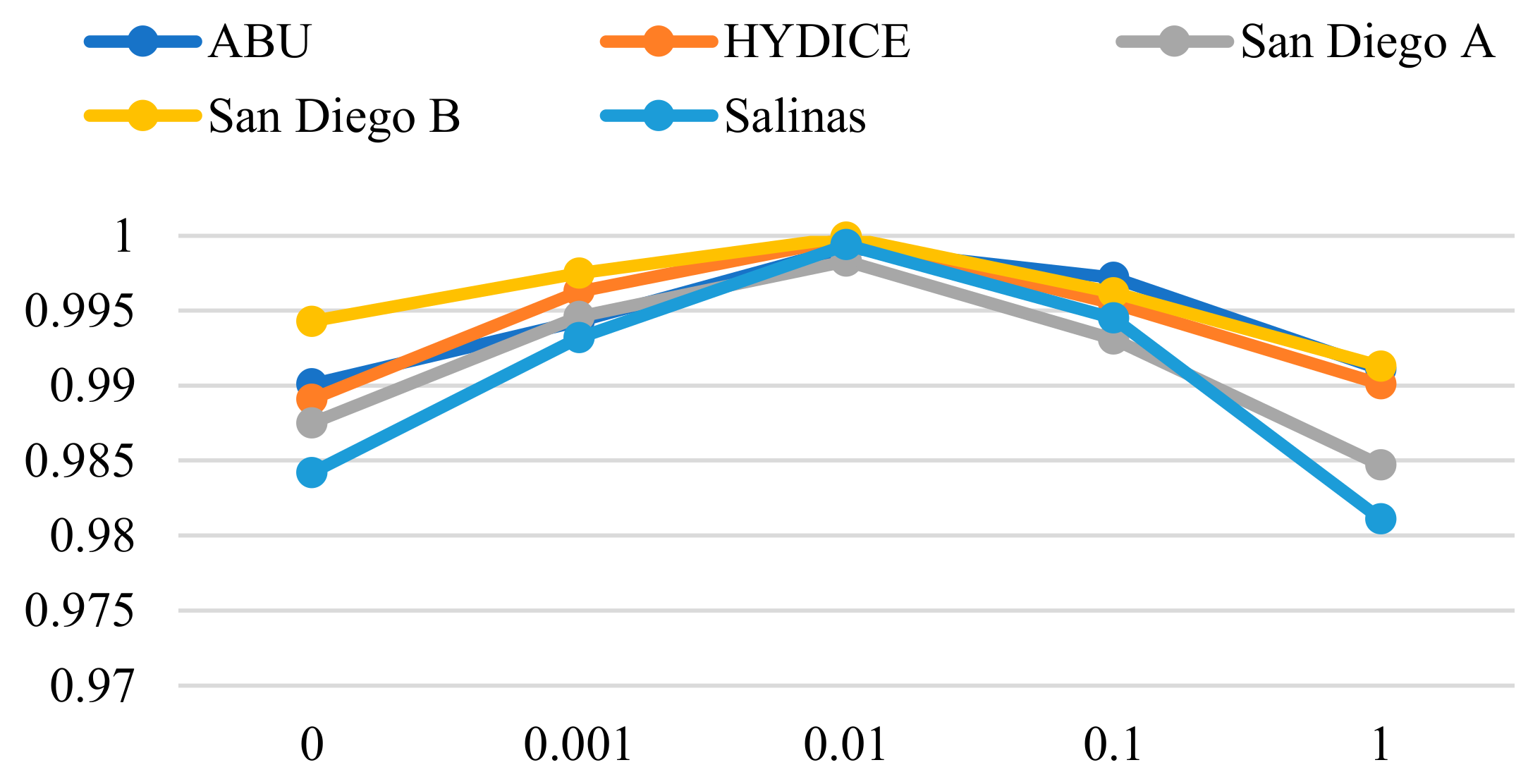
3.1.3. Parameter Setting

To validate the effectiveness of our proposed method, we compared it with seven other methods: four traditional methods, CEM [11], ACE, OSP [13], and MF; two convolution-based methods, SFCTD [29] and TSCNTD [15]; and a metric learning-based method, TSTTD [19].

All experiments were under the pytorch 1.13.1 environment with an Intel, Santa Clara, CA, USA, i5-13490f CPU, an NVIDIA, Santa Clara, CA, USA, GeForce RTX 4060Ti 16 GB GPU, and 32 GB memory.

To ensure we can divide the spectrum into integer patches, we set the patch size according to the number of bands in the spectral mask data augmentation network. The number of bands in ABU-urban-2, HYDICE, San Diego A, San Diego B, and Salinas is 207, 162, 189, 189, and 224, respectively, so the patch sizes were set to 3, 3, 7, 7, and 4 and the number of patches was 69, 54, 27, 27, and 56. D was set to 256. The batch size, learning rate, and epoch were set to 32, 0.001, and 300, using the Adam optimizer, respectively. The mask ratios were set to 25%, 50%, 75%, 85%, and 95%, respectively, and 75% yielded the best results. The β were set to 0, 0.001, 0.01, 0.1, and 1, respectively, and 0.01 obtained the best results.

In the multi-scale spectral metric network, we used the batch size as 32, the learning rate as 0.001, and the epoch as 200, also using the Adam optimizer.

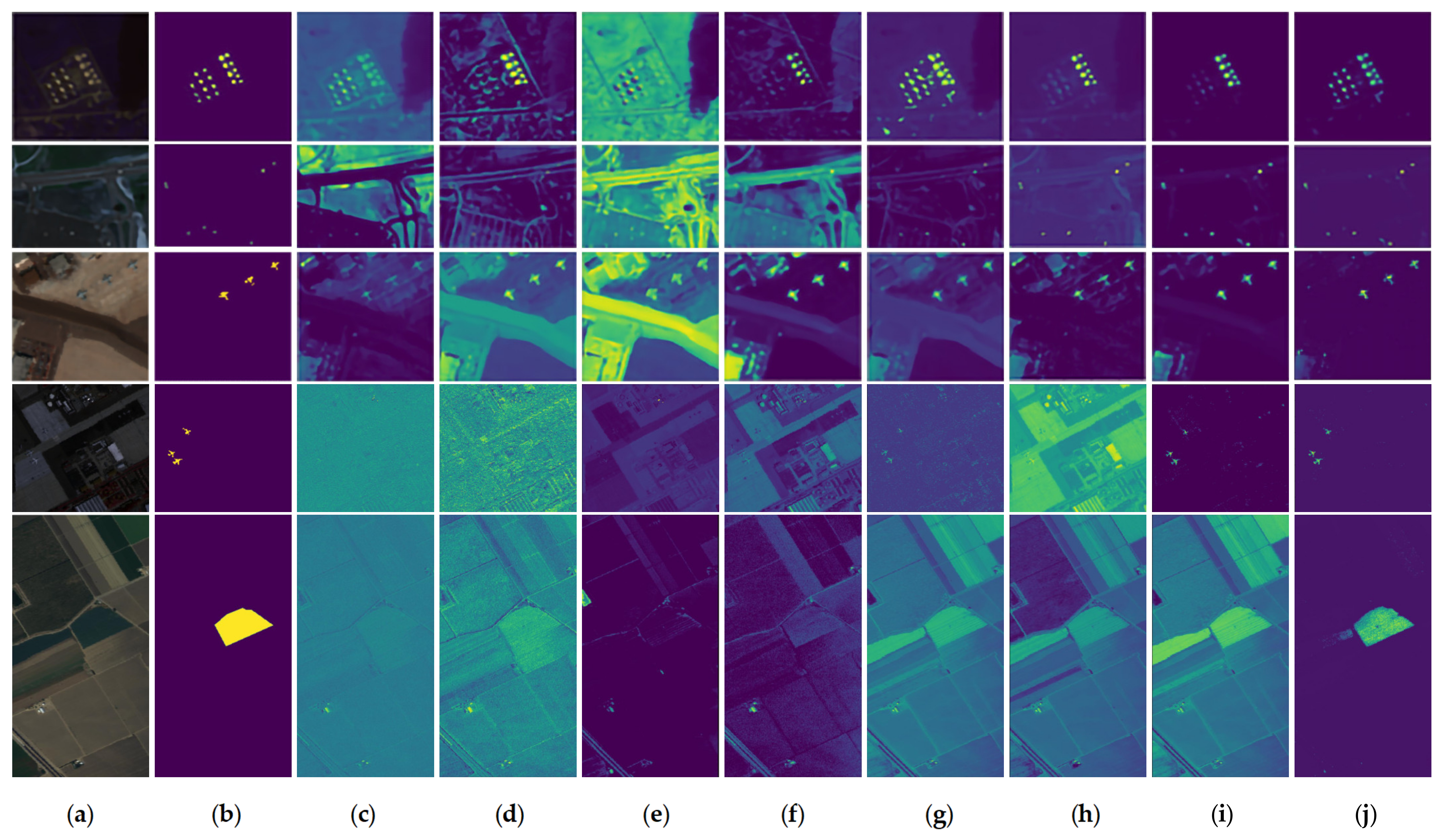
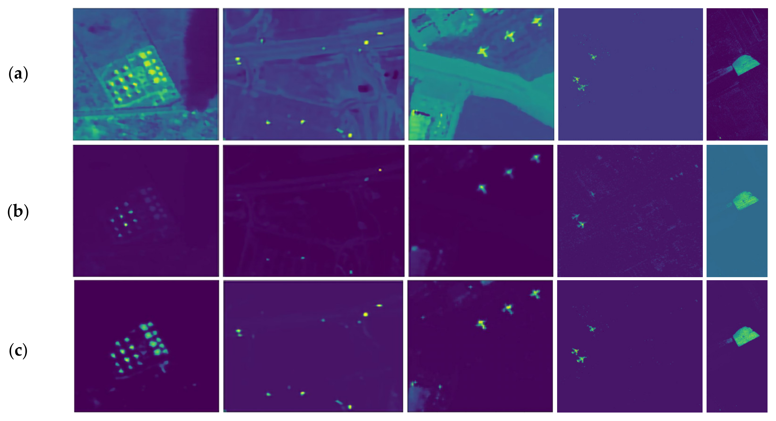
3.2. Comparison of the Experimental Results

The visual detection result, AUC values, ROC curves, and target-background separation maps are compared to verify the effectiveness of our proposed method.

Figure 5 shows the visual detection result of different methods. Traditional ACE and OSP methods perform worse than others in terms of background suppression and target detection, especially in the ABU and San Diego B dataset. CEM and MF have a better target detection result and can detect part of the target. However, they cannot suppress background, which leads to the detection of the background as the target. Deep learning-based SFCTD and TSCNTD methods are good for localized feature extraction and can identify the target accurately on ABU and HYDICE datasets. However, the background suppression is poor in San Diego A, San Diego B, and Salinas datasets due to the loss of spectral information during the pooling process. Triplet Net-based metric learning generated better detection results than deep learning-based methods and obtained better background suppression in five datasets. However, it misses too many target pixels, especially in the ABU dataset. Compared to other methods, our method showed better target detection result and background suppression on five datasets.

Figure 6 represents a comparison of the performances using target-background separability maps. The higher the target, the better the detection performance of the target. Similarly, the lower of background, the better the suppression of the background. The greater the difference between target and background, the better the separability of the target and background. Traditional methods are less effective than other methods in separating target and background. Convolution-based methods suppress the background on ABU, HYDICE, and San Diego A datasets but fail to distinguish between target and background on San Diego B and Salinas. The background suppression effect of our method on the ABU and HYDICE datasets is similar to TSTTD, which almost completely suppresses the background. However, the separation of target and background is better than TSTTD. Our method had the best background suppression effect for the San Diego A and San Diego B datasets.

Figure 7 represents a comparison of the ROC curve of different methods. The closer the ROC curve is to the upper left corner, the better the performance of the method. Our method is closer to the upper left corner in five datasets, especially on the San Diego B dataset. Other methods do not perform well in San Diego B, but our method is almost a straight line close to 1.

Table 2. AUC value comparison of different target detectors on five datasets.

Methods	ABU	HYDICE	San Diego A	San Diego B	Salinas
CEM	0.9842	0.6812	0.9902	0.4974	0.8853
ACE	0.7554	0.7103	0.9830	0.6346	0.9409
OSP	0.9133	0.7935	0.6735	0.2061	0.7896
MF	0.6685	0.9176	0.9753	0.7142	0.8431
SFCTD	0.9965	0.9972	0.9937	0.8824	0.9662
TSCNTD	0.9934	0.9499	0.9924	0.7727	0.9504
TSTTD	0.9935	0.9979	0.9959	0.9817	0.9685
Ours	0.9992	0.9998	0.9983	0.9999	0.9994

presents the comparison of the AUC value of all methods on five datasets, where a greater AUC value indicates a better detection performance. The traditional methods are inconsistent and can only provide good results on some datasets. For example, ACE performs well on San Diego A and Salinas dataset but not on ABU and HYDICE. SFCTD, TSCNTD, and TSTTD generated similar results on ABU, HYDICE, San Diego A and Salinas datasets, which are more robust and accurate. The proposed method obtained the highest AUC values for five datasets, demonstrating its effectiveness in target detection.

3.3. Experimental Setup

We selected mask ratios of 25%, 50%, 75%, 85%, and 95% to augment the data for five datasets, and the augmentation results for a batch were obtained, as shown in Figure 8. From the figure, it can be observed that when the mask ratio is too low, like 25%, 50%, the model cannot learn the information of the prior spectrum, resulting in excessive noise in augmented targets. When the mask ratio is too high, like 85% or 95%, the model confuses the prior spectra with background spectrum, resulting in augmented curves trending in different directions. When the mask ratio is 75%, better results can be obtained.

This is because with a low mask ratio, missing patches can be inferred from neighboring patches. The model will rely on this redundancy and fail to learn useful feature representations. And low mask ratio means the self-supervised task is not challenging enough to motivate the model to learn more advanced features. Although a high mask ratio is more challenging and forces the model to learn more robust feature representations, when the mask ration is too high, too much information of the prior spectrum is lost, making it difficult to accurately reconstruct the original spectrum. Experiments have shown that a mask ratio of 75% achieves the optimal balance. It ensures the task is difficult enough to promote meaningful learning while retaining enough information to learn useful feature representations.

Table 3. AUC value comparison of different mask ratios on five datasets.

Mask Ratio	ABU	HYDICE	San Diego A	San Diego B	Salinas
25%	0.8611	0.8731	0.8581	0.9903	0.9930
50%	0.8827	0.8628	0.8603	0.9971	0.9988
75%	0.9992	0.9998	0.9983	0.9999	0.9994
85%	0.9951	0.9732	0.9903	0.9892	0.9941
95%	0.9916	0.8755	0.7114	0.9867	0.9923

presents the AUC value of different mask ratios on five datasets. From the table, it can be seen that the detection accuracy is highest when the mask ratio is 75%.

To explore the effect of β, we compared the detection accuracy when β was 0, 0.001, 0.01, 0.1, and 1, as shown in Figure 9. When β is 0.001 or 0.01, better detection results can be obtained than for β as 0 because when no inter-class difference amplification operator was added.

However, when β is 0.1 or 1, it will influence the model excessively about the distance between the background and a prior spectrum and ignore the distance between the positive and negative samples, reducing the detection accuracy. As can be seen from the figure, when β was 0.01, better detection results can be obtained.

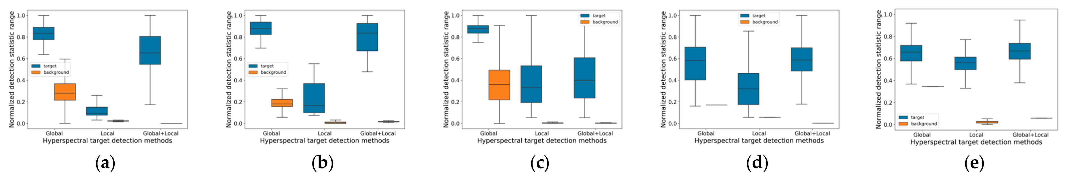
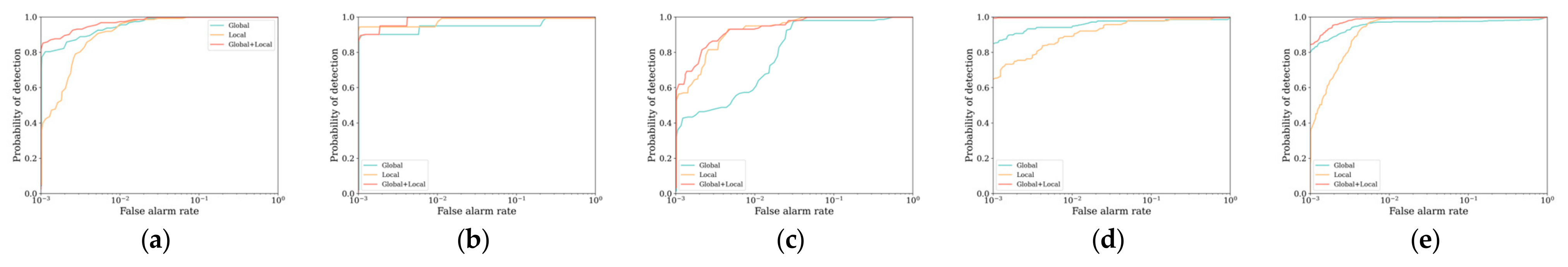
3.4. Ablation Experiments

The ablation experiments for verifying the global and local feature extraction parts in the multi-scale spectral metric network are carried out, with a mask ratio of 75% and β of 0.01.

Figure 10 shows the detection maps using global, local, and combined global and local parts, respectively.

The global feature extraction network captures the difference between the target and the background as a whole. However, due to the neglect of local details, it cannot effectively distinguish the target from the background when the target spectrum is similar to the background, resulting in weak background suppression, as shown in Figure 10a.

In contrast, a local feature extraction network can ignore the irrelevant global information and focus on a small range of spectral features that help distinguish the target from the background. The target detection performance is degraded due to the loss of target features in the global view, as shown in Figure 10b.

Combining the global and local feature extraction network can both retain the extensive contextual information provided by global features and utilize local features to enhance the sensitivity to subtle changes, thus improving the accuracy of target detection and the ability of background suppression, as shown in Figure 10c.

Figure 11 and Figure 12 compare the results of global, local, and combined global and local parts in terms of target-background separation maps and ROC curves, respectively. When the global feature extraction part was used, the target detection is better, but background suppression is worse. When only using the local feature extraction part, the target detection is worse and the background suppression is better. When the local and global modules were used together, the target and background were the furthest apart and could accurately distinguish the target from the background.

Table 4. AUC value comparison of ablation experiments on five datasets.

Global	Local	ABU	HYDICE	San Diego A	San Diego B	Salinas
√		0.9982	0.9881	0.9828	0.9911	0.9855
	√	0.9972	0.9994	0.9973	0.9906	0.9978
√	√	0.9992	0.9998	0.9983	0.9999	0.9994

presents a comparison of AUC values obtained from global, local, and combined global and local parts on five datasets. For the ABU and San Diego B datasets, only using global feature extraction part provided better results than only using local feature extraction part because the background is not too complicated. The highest detection accuracy was obtained when combining both global and local feature extraction parts.

4. Discussion

In the public datasets, we found that the spectral trends of the target and the surrounding background are almost the same, with only minor local differences. To address this issue, we propose HTD-DA, which achieves extremely high AUC values (close to 0.9999 on some datasets) in our experiments, indicating that the model performs extremely well in distinguishing the background from the target.

There are still some problems in our modeling. Using a traditional MAE-based network to generate target samples is simple and feasible, but the feature extraction capability is limited. Due to the high dimensionality of HSI, the training process is slower using a triplet network.

With the development of imaging technology, the spatial resolution of hyperspectral images can reach 1 m, and the size can be up to 1000 × 1000 pixels. If multiple images are stitched together, the image size can be even higher. In this case, HTD has some challenges and potential problems in practical applications.

• The data amount is too large, so processing these data requires not only efficient algorithms but also powerful computational capabilities to support fast analysis;
• Factors such as light, weather, and noise are difficult to control, which challenges the robustness of the algorithm.

5. Conclusions

In this study, we proposed an HTD method based on data arguments. We developed a masked spectral data augmentation network to generate more realistic target samples that learn spectral variability through masks. Simultaneously, we developed a multi-scale spectral metric network to learn the minor differences and overall trends between target and background spectra, improving the ability to discriminate between targets and suppress backgrounds.

Finally, we introduced IDATL to keep the target close to the prior spectrum and away from the background, which makes the background progressively less distant from the prior spectrum. Experiments were conducted on five datasets to verify their effectiveness.

In the future, the MAE-based network can be improved to enhance the spectral variability extraction ability and generate more realistic spectral curves. Difficult sample mining techniques can be used to select more valuable triplet training sets, improving the training efficiency.

References

1. Lu, B.; Dao, P.; Liu, J.; He, Y.; Shang, J. Recent Advances of Hyperspectral Imaging Technology and Applications in Agriculture. Remote Sens. 2020, 12, 2659. [Google Scholar] [CrossRef]
2. Wang, S.; Guan, K.; Zhang, C.; Lee, D.; Margenot, A.J.; Ge, Y.; Peng, J.; Zhou, W.; Zhou, Q.; Huang, Y. Using Soil Library Hyperspectral Reflectance and Machine Learning to Predict Soil Organic Carbon: Assessing Potential of Airborne and Spaceborne Optical Soil Sensing. Remote Sens. Environ. 2022, 271, 112914. [Google Scholar] [CrossRef]
3. Almeida, D.R.A.D.; Broadbent, E.N.; Ferreira, M.P.; Meli, P.; Zambrano, A.M.A.; Gorgens, E.B.; Resende, A.F.; De Almeida, C.T.; Do Amaral, C.H.; Corte, A.P.D.; et al. Monitoring Restored Tropical Forest Diversity and Structure through UAV-Borne Hyperspectral and Lidar Fusion. Remote Sens. Environ. 2021, 264, 112582. [Google Scholar] [CrossRef]
4. Makki, I.; Younes, R.; Francis, C.; Bianchi, T.; Zucchetti, M. A Survey of Landmine Detection Using Hyperspectral Imaging. ISPRS J. Photogramm. Remote Sens. 2017, 124, 40–53. [Google Scholar] [CrossRef]
5. Hou, Y.; Zhang, Y.; Yao, L.; Liu, X.; Wang, F. Mineral Target Detection Based on MSCPE_BSE in Hyperspectral Image. In Proceedings of the 2016 IEEE International Geoscience and Remote Sensing Symposium (IGARSS), Beijing, China, 10–15 July 2016; pp. 1614–1617. [Google Scholar]
6. Zhang, L.; Ma, J.; Fu, B.; Lin, F.; Sun, Y.; Wang, F. Improved Central Attention Network-Based Tensor RX for Hyperspectral Anomaly Detection. Remote Sens. 2022, 14, 5865. [Google Scholar] [CrossRef]
7. Manolakis, D.; Truslow, E.; Pieper, M.; Cooley, T.; Brueggeman, M. Detection Algorithms in Hyperspectral Imaging Systems: An Overview of Practical Algorithms. IEEE Signal Process. Mag. 2014, 31, 24–33. [Google Scholar] [CrossRef]
8. Chang, C.I. Spectral Information Divergence for Hyperspectral Image Analysis. In Proceedings of the IEEE 1999 International Geoscience and Remote Sensing Symposium. IGARSS’99 (Cat. No.99CH36293), Hamburg, Germany, 28 June–2 July 1999; Volume 1, pp. 509–511. [Google Scholar]
9. Kruse, F.A.; Lefkoff, A.B.; Boardman, J.W.; Heidebrecht, K.B.; Shapiro, A.T.; Barloon, P.J.; Goetz, A.F.H. The Spectral Image Processing System (SIPS)-Interactive Visualization and Analysis of Imaging Spectrometer Data. AIP Conf. Proc. 1993, 283, 192–201. [Google Scholar]
10. Zou, Z.; Shi, Z. Hierarchical Suppression Method for Hyperspectral Target Detection. IEEE Trans. Geosci. Remote Sens. 2016, 54, 330–342. [Google Scholar] [CrossRef]
11. Yang, X.; Chen, J.; He, Z. Sparse-SpatialCEM for Hyperspectral Target Detection. IEEE J. Sel. Top. Appl. Earth Obs. Remote Sens. 2019, 12, 2184–2195. [Google Scholar] [CrossRef]
12. Yang, X.; Zhao, M.; Shi, S.; Chen, J. Deep Constrained Energy Minimization for Hyperspectral Target Detection. IEEE J. Sel. Top. Appl. Earth Obs. Remote Sens. 2022, 15, 8049–8063. [Google Scholar] [CrossRef]
13. Chang, C.I. Orthogonal Subspace Projection (OSP) Revisited: A Comprehensive Study and Analysis. IEEE Trans. Geosci. Remote Sens. 2005, 43, 502–518. [Google Scholar] [CrossRef]
14. Chen, Y.; Nasrabadi, N.M.; Tran, T.D. Sparse Representation for Target Detection in Hyperspectral Imagery. IEEE J. Sel. Top. Signal Process. 2011, 5, 629–640. [Google Scholar] [CrossRef]
15. Zhu, D.; Du, B.; Zhang, L. Two-Stream Convolutional Networks for Hyperspectral Target Detection. IEEE Trans. Geosci. Remote Sens. 2021, 59, 6907–6921. [Google Scholar] [CrossRef]
16. Gao, L.; Chen, L.; Liu, P.; Jiang, Y.; Xie, W.; Li, Y. A Transformer-Based Network for Hyperspectral Object Tracking. IEEE Trans. Geosci. Remote Sens. 2023, 61, 5528211. [Google Scholar] [CrossRef]
17. Zhang, X.; Gao, K.; Wang, J.; Hu, Z.; Wang, H.; Wang, P.; Zhao, X.; Li, W. Self-Supervised Learning with Deep Clustering for Target Detection in Hyperspectral Images with Insufficient Spectral Variation Prior. Int. J. Appl. Earth Obs. Geoinf. 2023, 122, 103405. [Google Scholar] [CrossRef]
18. Koch, G.; Zemel, R.; Salakhutdinov, R. Siamese Neural Networks for One-Shot Image Recognition. In Proceedings of the 32nd International Conference on Machine Learning, Lille, France, 6–11 July 2015. [Google Scholar]
19. Jiao, J.; Gong, Z.; Zhong, P. Triplet Spectralwise Transformer Network for Hyperspectral Target Detection. IEEE Trans. Geosci. Remote Sens. 2023, 61, 5519817. [Google Scholar] [CrossRef]
20. Qin, H.; Xie, W.; Li, Y.; Jiang, K.; Lei, J.; Du, Q. Weakly Supervised Adversarial Learning via Latent Space for Hyperspectral Target Detection. Pattern Recognit. 2023, 135, 109125. [Google Scholar] [CrossRef]
21. Rao, W.; Gao, L.; Qu, Y.; Sun, X.; Zhang, B.; Chanussot, J. Siamese Transformer Network for Hyperspectral Image Target Detection. IEEE Trans. Geosci. Remote Sens. 2022, 60, 5526419. [Google Scholar] [CrossRef]
22. Qin, J.; Fang, L.; Lu, R.; Lin, L.; Shi, Y. ADASR: An Adversarial Auto-Augmentation Framework for Hyperspectral and Multispectral Data Fusion. IEEE Geosci. Remote Sens. Lett. 2023, 20, 5002705. [Google Scholar] [CrossRef]
23. Zhang, M.; Wang, Z.; Wang, X.; Gong, M.; Wu, Y.; Li, H. Features Kept Generative Adversarial Network Data Augmentation Strategy for Hyperspectral Image Classification. Pattern Recognit. 2023, 142, 109701. [Google Scholar] [CrossRef]
24. Wang, W.; Chen, Y.; He, X.; Li, Z. Soft Augmentation-Based Siamese CNN for Hyperspectral Image Classification with Limited Training Samples. IEEE Geosci. Remote Sens. Lett. 2022, 19, 5508505. [Google Scholar] [CrossRef]
25. Gao, Y.; Feng, Y.; Yu, X. Hyperspectral Target Detection with an Auxiliary Generative Adversarial Network. Remote Sens. 2021, 13, 4454. [Google Scholar] [CrossRef]
26. He, K.; Chen, X.; Xie, S.; Li, Y.; Dollár, P.; Girshick, R. Masked Autoencoders Are Scalable Vision Learners. In Proceedings of the IEEE/CVF Conference on Computer Vision and Pattern Recognition (CVPR), New Orleans, LA, USA, 18–24 June 2022. [Google Scholar]
27. Wang, Y.; Chen, X.; Wang, F.; Song, M.; Yu, C. Meta-Learning Based Hyperspectral Target Detection Using Siamese Network. IEEE Trans. Geosci. Remote Sens. 2022, 60, 5527913. [Google Scholar] [CrossRef]
28. Zhang, X.; Gao, K.; Wang, J.; Hu, Z.; Wang, H.; Wang, P. Siamese Network Ensembles for Hyperspectral Target Detection with Pseudo Data Generation. Remote Sens. 2022, 14, 1260. [Google Scholar] [CrossRef]
29. Gao, H.; Zhang, Y.; Chen, Z.; Xu, F.; Hong, D.; Zhang, B. Hyperspectral Target Detection via Spectral Aggregation and Separation Network With Target Band Random Mask. IEEE Trans. Geosci. Remote Sens. 2023, 61, 5515516. [Google Scholar] [CrossRef]
30. Jiao, J.; Gong, Z.; Zhong, P. Dual-Branch Fourier-Mixing Transformer Network for Hyperspectral Target Detection. Remote Sens. 2023, 15, 4675. [Google Scholar] [CrossRef]
31. Chen, X.; Ding, M.; Wang, X.; Xin, Y.; Mo, S.; Wang, Y.; Han, S.; Luo, P.; Zeng, G.; Wang, J. Context Autoencoder for Self-Supervised Representation Learning. Int. J. Comput. Vis. 2024, 132, 208–223. [Google Scholar] [CrossRef]
32. Ly, S.T.; Lin, B.; Vo, H.Q.; Maric, D.; Roysam, B.; Nguyen, H.V. Cellular Data Extraction from Multiplexed Brain Imaging Data Using Self-Supervised Dual-Loss Adaptive Masked Autoencoder. Artif. Intell. Med. 2024, 151, 102828. [Google Scholar] [CrossRef]
33. Guo, Q.; Cen, Y.; Zhang, L.; Zhang, Y.; Huang, Y. Hyperspectral Anomaly Detection Based on Spatial–Spectral Cross-Guided Mask Autoencoder. IEEE J. Sel. Top. Appl. Earth Obs. Remote Sens. 2024, 17, 9876–9889. [Google Scholar] [CrossRef]
34. Boutros, F.; Damer, N.; Kirchbuchner, F.; Kuijper, A. Self-Restrained Triplet Loss for Accurate Masked Face Recognition. Pattern Recognit. 2022, 124, 108473. [Google Scholar] [CrossRef]
35. Xie, W.; Wu, H.; Tian, Y.; Bai, M.; Shen, L. Triplet Loss With Multistage Outlier Suppression and Class-Pair Margins for Facial Expression Recognition. IEEE Trans. Circuits Syst. Video Technol. 2022, 32, 690–703. [Google Scholar] [CrossRef]
36. Chen, J.; Lai, H.; Geng, L.; Pan, Y. Improving Deep Binary Embedding Networks by Order-Aware Reweighting of Triplets. arXiv 2018, arXiv:1804.06061. [Google Scholar]
Figure 1. Spectrum of the target and background. (a) The pseudo figure of the urban-2 dataset, with targets in red. (b) Enlarged view of the red box in (a) and select one target and three backgrounds. (c) The spectrum of the target and three backgrounds; the black boxes are the parts of the target that are slightly different from the background.
Remotesensing 17 01097 g001
Figure 2. Structure of the MAE network. Black indicates masked patch, green and orange indicate encoder and decoder patches, respectively.
Remotesensing 17 01097 g002
Figure 3. Overall architecture of the proposed HTD-DA.
Remotesensing 17 01097 g003
Figure 4. Structure of the CET block.
Remotesensing 17 01097 g004
Figure 5. Experimental datasets and detection maps of competing methods. (a) False-color image. (b) Ground truth. (c) CEM. (d) ACE. (e) OSP. (f) MF. (g) SFCTD. (h) TSCNTD. (i) TSTTD. (j) Ours. From top to bottom are ABU, HYDICE, San Diego A, San Diego B, Salinas datasets, respectively.
Remotesensing 17 01097 g005
Figure 6. Target background separation maps of competing methods on five datasets. (a) ABU. (b) HYDICE. (c) San Diego A. (d) San Diego B. (e) Salinas.
Remotesensing 17 01097 g006
Figure 7. ROC curves of competing methods on five datasets. (a) ABU. (b) HYDICE. (c) San Diego A. (d) San Diego B. (e) Salinas.
Remotesensing 17 01097 g007
Figure 8. A batch target spectrums obtained with different mask ratios on five datasets. (a) Prior spectrum, (b) 25% mask ratio, (c) 50% mask ratio, (d) 75% mask ratio, (e) 85% mask ratio, (f) 95% mask ratio. From top to bottom: ABU, HYDICE, San Diego A, San Diego B, and Salinas.
Remotesensing 17 01097 g008
Figure 9. Detection accuracy obtained with different β values on five datasets.
Remotesensing 17 01097 g009
Figure 10. Detection maps of the ablation experiment on five datasets. (a) Global module. (b) Local module. (c) Combined global and local module. From left to right: ABU, HYDICE, San Diego A, San Diego B and Salinas.
Remotesensing 17 01097 g010
Figure 11. Target-background separation maps of ablation experiment on five datasets. (a) ABU (b) HYDICE. (c) San Diego A. (d) San Diego B. (e) Salinas.
Remotesensing 17 01097 g011
Figure 12. ROC curves of ablation experiment on five datasets. (a) ABU. (b) HYDICE. (c) San Diego A. (d) San Diego B. (e) Salinas.
Remotesensing 17 01097 g012