Detection of Parabolic Antennas in Satellite Inverse Synthetic Aperture Radar Images Using Component Prior and Improved-YOLOv8 Network in Terahertz Regime

Abstract

Inverse Synthetic Aperture Radar (ISAR) images of space targets and their key components are very important. However, this method suffers from numerous drawbacks, including a low Signal-to-Noise Ratio (SNR), blurred edges, significant variations in scattering intensity, and limited data availability, all of which constrain its recognition capabilities. The terahertz (THz) regime has reflected excellent capacity for space detection in terms of showing the details of target structures. However, in ISAR images, as the observation aperture moves, the imaging features of the extended structures (ESs) undergo significant changes, posing challenges to the subsequent recognition performance. In this paper, a parabolic antenna is taken as the research object. An innovative approach for identifying this component is proposed by using the advantages of the Component Prior and Imaging Characteristics (CPICs) effectively. In order to tackle the challenges associated with component identification in satellite ISAR imagery, this study employs the Improved-YOLOv8 model, which was developed by incorporating the YOLOv8 algorithm, an adaptive detection head known as the Dynamic head (Dyhead) that utilizes an attention mechanism, and a regression box loss function called Wise Intersection over Union (WIoU), which addresses the issue of varying sample difficulty. After being trained on the simulated dataset, the model demonstrated a considerable enhancement in detection accuracy over the five base models, reaching an mAP50 of 0.935 and an mAP50-95 of 0.520. Compared with YOLOv8n, it improved by 0.192 and 0.076 in mAP50 and mAP50-95, respectively. Ultimately, the effectiveness of the suggested method is confirmed through the execution of comprehensive simulations and anechoic chamber tests.

1. Introduction

In response to the needs of scientific and economic advancement, an extensive array of space-based systems, including space stations and satellites, have been deployed into the vast expanse of space [1,2]. So far, optical telescopes [3,4] and ground-based radars [5] are the main detection sensors of satellites in orbit. High-resolution observations of celestial bodies are feasible with optical telescopes; however, the clarity of the resulting images is significantly influenced by the lighting circumstances. Ground-based radar systems are capable of conducting continuous, round-the-clock surveillance and ISAR imaging for space objects, and they have emerged as the predominant method for such oversight. However, they still have some drawbacks. Initially, the limitation of transmission power poses challenges in detecting High Earth Orbit (HEO) satellite targets and small satellite targets, as the extended transmission distance and their low Radar Cross Section (RCS) contribute to their difficulty in being observed. The second challenge is that current ground-based radar systems typically operate in frequency bands below the W-band. This choice is made to mitigate the effects of atmospheric attenuation, which can degrade radar signals as they pass through the atmosphere. However, operating at lower frequencies also comes with a trade-off: it limits the imaging resolution. As a result, it is not possible to achieve detailed imaging and recognition of space objects down to the component level, meaning that the fine details of the satellite structure or individual components may not be discernible with these radar systems. Thirdly, when observing the target in HEO, the change in the elevation angle of the Line of Sight (LOS) is not enough to match the change in the azimuth angle, resulting in an unbalanced distribution of attitude parameters. Furthermore, accurately confirming the status of the target requires a detailed understanding of the component information, which the current methods are unable to fully provide. Furthermore, certain key structural features of the object may be susceptible to fading and blurring during radar imaging. This can be problematic for intelligent image interpretation, as the loss of clarity in these features may hinder the ability to accurately identify and analyze the object’s components or characteristics. Such limitations can affect the overall effectiveness of radar surveillance and the subsequent analysis of space objects.

Terahertz (THz) waves are a form of electromagnetic radiation characterized by wavelengths that span from 3 mm (mm) to 30 $\mathsf{\mu }$m (µm). This range corresponds to frequencies that fall between 0.1 terahertz (THz) and 10 THz. The use of THz waves in various applications is of interest due to their unique properties, such as their ability to penetrate certain materials without significant attenuation, making them useful for non-destructive testing and imaging as well as for communication and sensing [6]. Since terahertz waves have a shorter wavelength than low-frequency microwaves, this allows terahertz waves to achieve high-resolution imaging at shorter synthetic apertures. In addition, the terahertz region has many unique characteristics, including but not limited to a certain anti-interference [7] and penetration [8], and is widely used in astronomical exploration and wireless communication [9,10,11]. A space-based terahertz radar imaging system is proposed because of the above advantages. Therefore, in the application scenario of high-resolution radar, the performance of terahertz radar imaging is expected to reflect the detailed characteristics of the key component structure of the target.

The parabolic antenna load, as we all know, is a key component of satellite communication systems, and accurate identification of parabolic antennas is important to condition assessment and function maintenance, and it provides favorable support for subsequent three-dimensional reconstruction and pointing estimation tasks. The basic scattering characteristics and imaging methods for the terahertz frequency band are thoroughly discussed in reference [12]. This study demonstrates that the number of scattering centers in a scene increases significantly with the presence of rough surfaces, which can degrade image quality. To address the image quality degradation caused by dense scattering centers, researchers have investigated terahertz imaging enhancement techniques based on sparse regularization [13] and machine learning [14]. These methods have been shown to effectively surpass the Rayleigh limit, which is a fundamental limit of resolution in traditional imaging techniques. When these imaging enhancement methods were first proposed, scholars aimed to achieve a level of detail in the object of interest that was as clear as optical images. This goal was driven by the desire to obtain highly resolved and detailed images, even in the presence of complex scattering environments that traditionally limit the clarity of terahertz images. Through our research, due to the special azimuth dependence of extended structures (ESs), the key extended structures of complex targets such as parabolic antennas may disappear and be discretized into specular points, edge pair-points, or ellipse arcs, which are quite different from optical images. Therefore, we need to propose a new image interpretation and translation method for parabolic antennas.

The Constant False Alarm Rate (CFAR) detection technique, a well-established method, is widely utilized for its straightforwardness and efficiency [15]. A robust CFAR detector, grounded in truncated maximum likelihood principles, is adeptly implemented in environments prone to outlier interference, demonstrating adequate computational efficiency [16]. Despite this, contemporary object detection approaches leveraging deep neural networks have outperformed traditional methods in both accuracy and speed [17,18,19,20]. Rotter et al. [21] developed two alternative systems that utilize the Single-Shot multibox Detector (SSD) and the Tiny YOLOv2 network for the automated detection of sinking funnels generated by underground coal mining. A method integrating Interferometric Synthetic Aperture Radar (InSAR) and Convolutional Neural Networks (CNNs) is proposed for the automatic identification of subsidence funnels caused by coal mining activities [22]. Yu et al. [23] introduced a lean model named Light You Only Look Once (YOLO)-Basin, which is designed for subsidence basin detection using the YOLOv5 network. Under the premise of key frames, a technology to estimate the parameters of a parabolic antenna is presented explicitly [24]. This method significantly reduces the computational complexity of the model and improves the accuracy of the model. In the terahertz frequency ban, by analyzing the sliding scattering center and cross-polarization imaging characteristics of parabolic antennas, an improved Hough transform method has been proposed for identifying parabolic antennas [25]. Through the analysis of the prior information of the components and their imaging characteristics, the literature effectively identifies the components and is able to successfully reconstruct them in the terahertz regime [26]. These advancements offer valuable insights that inform the development of our proposed approach.

In this article, a novel method for detecting parabolic antennas is proposed. The main idea lies in the good use of CPICs as well as an improved-YOLOv8 object detection network. To make full use of the CPICs of the component, four objects are to be detected: the satellite body and the three statuses of the parabolic antenna, namely, specular point, edge-pair points, and ellipse arc. We not only give the characteristics of the parabolic antenna when imaging it alone but also realize the identification of parabolic antenna based on the detection of satellite. This article makes the following key contributions:

(1) Inserting the CPICs of a parabolic antenna into the object detection network, a new method for parabolic antenna detection is proposed, including two steps: determining the component prior and detecting the three statuses of the parabolic antenna.

(2) Using the scattering prior which is obtained by electromagnetic simulations, the imaging characteristics of the parabolic antennas of satellites are analytically determined.

(3) Compared with previous target detection networks, the proposed method achieves better detection effects for key components.

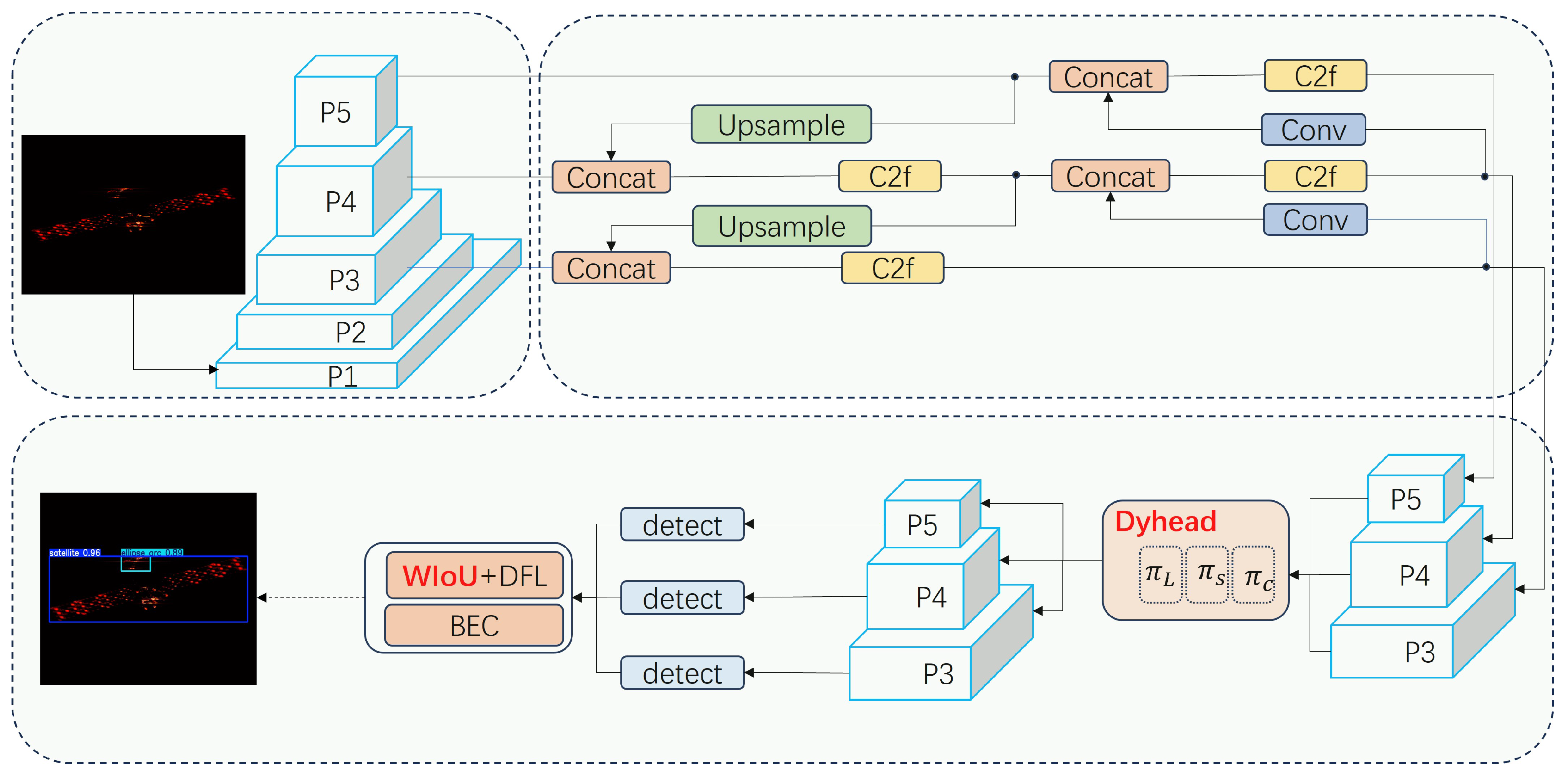
The proposed method’s overall structure is depicted in Figure 1. In Figure 1, firstly, we obtain the original echo data of the satellite model through electromagnetic simulation software, as mentioned in “Raw data of satellite echoes”. Then, using the classical RD imaging algorithm, we obtain the “Imaging result of satellite”. Additionally, by utilizing “Analyzing the ICPC” of the parabolic antenna, we extract the imaging characteristics of the parabolic antenna, providing an improvement approach for the next deep learning model. Finally, combining the ICPC of the parabolic antenna, we convert the recognition of the parabolic antenna into the detection of “Specular reflection point”, “Edge pair-point”, and “Ellipse arc”, and we execute “Training the Networks”. The organization of the remainder of this article proceeds as follows. In Section 2, the THz imaging characters of parabolic antennas are discussed. In Section 3, the Improved-YOLOv8 network is illustrated in detail. The electromagnetic simulation results and relevant analysis are provided, and the results are verified by the anechoic chamber experiment in Section 4. Finally, we give the conclusions of this paper in Section 5.

2. THz Imaging Character of Parabolic Antennas

The observation geometry of the spatial target for the space-based terahertz radar is depicted in Figure 2. The LOS vector links the $O_{Target}$ and $O_{Radar}$ points. In the case of a three-axis stabilized space target, its orientation remains constant with respect to the coordinate system of the target, and the projection onto the imaging plane is determined by the corresponding LOS angles of the radar.

The radar LOS can be represented as:

$$LOS={\left[\begin{array}{ccc}cos\theta cos\phi ,& cos\theta sin\phi ,& sin\theta \end{array}\right]}^{\mathrm{T}}$$

(1)

where the superscript T denotes transposition, $\theta \in [-{90}^{\circ },{90}^{\circ })$, and $\phi \in [-{180}^{\circ },{180}^{\circ })$, which represent the elevation angles and azimuth angles, respectively. The orientation of a parabolic antenna can be expressed as follows:

$$k={\left[\begin{array}{ccc}cos\beta cos\alpha ,& cos\beta sin\alpha ,& sin\beta \end{array}\right]}^{\mathrm{T}}$$

(2)

where k is usually called the normal vector and $\alpha \in [-{180}^{\circ },{180}^{\circ })$ and $\beta \in [-{90}^{\circ },{90}^{\circ })$ represent the yaw angle and the pitch angle, respectively. The R-axis and the D-axis of the ISAR plane are determined by the LOS vector and derivation LOS vector, respectively [27]. Since the projection relationship is not the key part of this article, we overlook its fussy details. It is important to recognize that all these angles can vary arbitrarily, leading to a complex issue. In reality, it is more common to focus on just a single rotational axis in order to achieve the highest possible imaging quality. After further analysis, we can see that the elevation and azimuth angles of the target relative to the radar’s LOS are, respectively, denoted as

$$\vartheta =\theta -\beta$$

(3)

$$\psi =\phi -\alpha$$

(4)

For the sake of analysis convenience, in the imaging setup of this paper, it is assumed that the elevation angle $\vartheta$ remains constant and only the rotation accumulation of the azimuth angle $\psi$ is considered to change. Without loss of generality, let $\alpha =0$, namely, the relative azimuth angle $\psi$ is equal to the $\phi$ angle.

We assume that the 2D ISAR imaging plane of the space target is composed of the R-axis and the D-axis, where the R-axis of the imaging plane is determined by the LOS vector, while the D-axis is defined based on the differentiation of the LOS vector. Given a point $M={[u,v,w]}^T$, which represents a 3D vector, its corresponding projection onto the 2D R–D imaging plane is referred to as $N={[r,d]}^T$. This projection relationship can be expressed as:

$$N=P·M$$

(5)

where P is the projection matrix, represented as

$$P=\left[\begin{array}{ccc}cos\theta cos\varphi & cos\theta sin\phi & sin\theta \\ P_{21}& P_{22}& cos\theta {\theta }^{\prime }\end{array}\right]$$

(6)

and $P_{21}$ and $P_{22}$ are denoted as

$$\left\{\begin{array}{c}{P}_{21}=-sin\theta cos\phi {\theta }^{\prime }-cos\theta sin\phi {\phi }^{\prime }\hfill \\ P_{22}=-sin\theta sin\phi {\theta }^{\prime }+cos\theta cos\phi {\phi }^{\prime }\hfill \end{array}\right.$$

(7)

where ${\theta }^{\prime }$ and ${\phi }^{\prime }$ represent the instantaneous velocities of the elevation and azimuth angles, respectively. Additionally, if the scatter point M is rotated along the $O_{Target}-UVW$ coordinate with angle ${\left[{\theta }_{\mu }{\theta }_{\nu }{\theta }_{\omega }\right]}^{\mathrm{T}}$, the rotated point $\widehat{M}$ is

$$\widehat{M}=R_W·R_V·R_U·M$$

(8)

where $R_U$, $R_V$, and $R_W$ are the rotation matrices along the $U-$, $V-$, and $W-$ axes, respectively. Specifically,

$$R_U=\left[\begin{array}{cccccc}& 1& & 0& & 0\\ & 0& & cos{\theta }_{\mu }& & -sin{\theta }_{\mu }\\ & 0& & sin{\theta }_{\mu }& & cos{\theta }_{\mu }\end{array}\right]$$

(9)

$$R_V=\left[\begin{array}{ccccc}cos{\theta }_{\nu }& & 0& & -sin{\theta }_{\nu }\\ 0& & 1& & 0\\ sin{\theta }_{\nu }& & 0& & cos{\theta }_{\nu }\end{array}\right]$$

(10)

$$R_W=\left[\begin{array}{cccc}cos{\theta }_{\omega }& -sin{\theta }_{\omega }& & 0\\ sin{\theta }_{\omega }& & cos{\theta }_{\omega }& & 0\\ 0& & 0& & 1\end{array}\right].$$

(11)

In this scenario, the projection relationship is

$$N=P·R_W·R_V·R_U·M=P^{\prime }·M$$

(12)

where $P^{\prime }=P·R_W·R_V·R_U$.

Moreover, in the geometric model of THz-ISAR imaging, the motion of the target relative to the radar can be independently decomposed into translational and rotational components. Taking into account the initial slant range and the instantaneous change in slant range due to translational motion, the instantaneous slant range $R_i\left(t_m\right)$ of scatter point i can be expressed as:

$$R_i\left(t_m\right)=r_0+r\left(t_m\right)+x_{i}sin\omega t_m+y_{i}cos\omega t_m$$

(13)

where $t_m$ denotes the slow time, $r_0$ represents the initial slant range, $r_m$ signifies the slant range of the target’s rotation center as it varies with the slow time, $x_i$ and $y_i$ are the coordinates of the i-th scatter point, and $\omega$ is the rotation speed of the target. It is assumed that the radar emits a linear frequency-modulated (LFM) signal:

$$s\left(\widehat{t};t_m\right)=\mathrm{rect}\left[{\displaystyle \frac{\widehat{t}}{T_p}}\right]·exp\left(j2\pi f_{c}t+j\pi \gamma {\widehat{t}}^2\right).$$

(14)

Following the delay time

$$\tau ={\displaystyle \frac{2R_i\left(t_m\right)}{c}},$$

(15)

the echo signal that has been acquired is

$$s_i(\widehat{t};t_m)=\mathrm{rect}\left[{\displaystyle \frac{\widehat{t}-2R_i\left(t_m\right)/c}{T_p}}\right]·exp\left\{j2\pi f_c\left[\widehat{t}-{\displaystyle \frac{2R_i\left(t_m\right)}{c}}\right]+j\pi {\gamma }_0{\left[\widehat{t}-{\displaystyle \frac{2R_i\left(t_m\right)}{c}}\right]}^2\right\}$$

(16)

where $T_p$ denotes the pulse duration, $f_c$ stands for the carrier frequency, and ${\gamma }_0$ indicates the frequency deviation of the linear frequency-modulated (LFM) signal. We proceed to perform dechirping and pulse compression on the received echo signal:

$$S(f_r;t_m)=\sum _{i=0}^{Q-1}\left\{{\sigma }_i·\mathrm{sinc}\left\{T_p\left[f_r+{\displaystyle \frac{2R_i\left(t_m\right)}{c}}\right]\right\}·exp\left[-j{\displaystyle \frac{4\pi f_c}{c}}{R}_i\left(t_m\right)\right]\right\}$$

(17)

where Q denotes the number of scatter points and ${\sigma }_i$ denotes the radar cross section of i-th scatter point.

Based on the imaging geometry above, the imaging characteristic of one ideal parabolic antenna is first analyzed.

The geometry of the paraboloid within the Cartesian coordinate system is depicted in Figure 3, and its equation could be presented in this manner:

$$x={\displaystyle \frac{y^2+z^2}{4K}},$$

(18)

where K represents the focal length. Given the rotational symmetry of the paraboloid, this study focuses on its projection onto the x–y plane, which forms a parabola. In Figure 3, the parabola is depicted as an orange curve. The diameter is represented by D, and $\phi$ denotes the angle between the electromagnetic wave transmitted by the radar and the y-axis. It is assumed that the scenario satisfies the far field condition, so the electromagnetic wave emitted by radar can be regarded as a plane wave. The focal point is denoted by G, and P is the specular reflected point on the parabola as it relates to the incident angle. $\rho$ is the distance between G and P, and $\beta$ is the angle between line segment GP and the y-axis. Since one of the parabola’s properties is that $\beta =2\phi$, the equation of the parabola can be formulated in this polar coordinate manner:

$$\rho ={\displaystyle \frac{2K}{1+cos\left(2\phi \right)}}.$$

(19)

Figure 3 illustrates that the location of the point of specular reflection moves along the parabola as the incident wave continuously varies angle, and the range of angle $\phi$ can be computed as follows:

$$\phi \in \left[-{\displaystyle \frac{1}{2}}arctan\left({\displaystyle \frac{8DF}{16K^2-D^2}}\right),{\displaystyle \frac{1}{2}}arctan\left({\displaystyle \frac{8DF}{16K^2-D^2}}\right)\right].$$

(20)

Owing to this distinctive feature, the paraboloid is classified as a sliding scattering center [28]. The point of specular reflection significantly impacts the Radar Cross Section (RCS). Additionally, the rim of the paraboloid contributes to the RCS [29]. Nonetheless, when the specular reflected point is present, this smaller part is often negligible. Therefore, the mirror-like scattering point is a characteristic of the paraboloidal imaging, in this case.

According to the analysis of the sliding scattering center of the parabolic antenna, the imaging characteristics of a parabolic antenna can be categorized into specular scattering points and non-specular scattering points. Furthermore, through observations from multiple simulation experiments, we have found that the non-specular scattering points can be divided into two main categories: edge pair-points and ellipse arc. To illustrate the imaging characteristic of parabolic antenna, we give an example of EM. The parameters of the parabolic antenna are as follows: radius = 25 cm, focal depth = 25 cm, edge width = 1 cm, and relative elevation angle $\psi ={10}^{\circ }$. Three typical observation apertures, AB, CD, and EF, are selected, and their imaging results are shown in Figure 4c–e, respectively. The images are presented in dB magnitude scale. The imaging result under the aperture AB has the one specular reflection point, whereas those of the apertures EF and CD have the scattered points about the edge of a paraboloid, which is consistent with the above theoretical analysis. Furthermore, it is observed that in Figure 4a,b, the amplitude discrepancies at the edge points are subject to substantial changes when the observation aperture is no longer aligned with the specular direction. This implies that the amplitude of the less intense scattered point could potentially exceed the dynamic range, resulting in it being obscured.

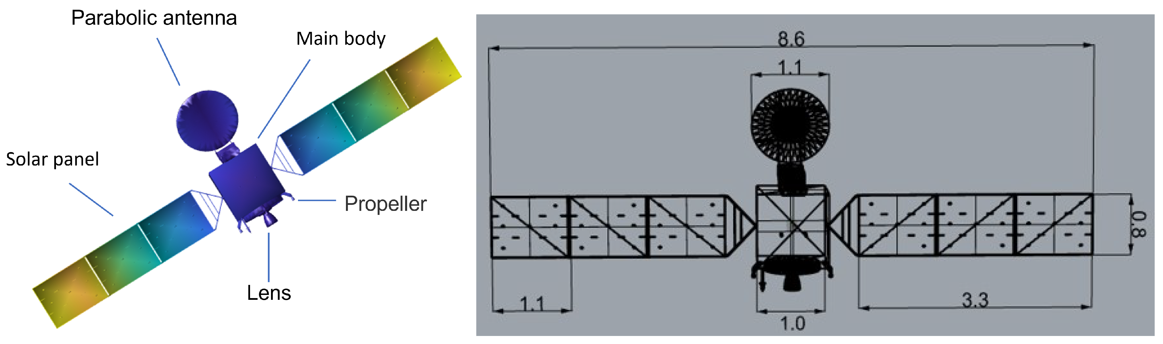
Therefore, the imaging properties of the satellite are analyzed by forward modeling and electromagnetic computations. In the case of the forward modeling, the satellite’s Computer-Aided Design (CAD) model and its geometry and size are depicted in Figure 5. In particular, the satellite model adopted in this paper has a total length of $8.6$ m, with each side of the sail panel measuring $3.3$ m in length and $0.8$ m in width and the diameter of the parabolic antenna being $1.1$ m, as illustrated in Figure 5. Dependent on the corporeal composition and shell curvatures listed in

Table 1. Scattering mechanism of each component of satellite.

Scattering Component	Description	Scattering Mechanism
Parabolic antenna	Dish-shaped structure that is designed to receive and transmit signals	Single/multiple reflection
Solar panel	Crucial component that provides electrical power to the satellite	Single/multiple reflection
Main body	Box-like structure that houses the majority of the satellite’s instruments, electronics, and systems	Single/multiple reflection
Lens	Cavity structure that is a key component in cameras or telescopes	Multiple reflection
Propeller	Cavity device that converts rotational motion into thrust	Multiple reflection

, five primary scattering elements are identified. Among these five elements, the parabolic antenna, solar panels, main body, propeller, and lens are clearly discernible in the imaging outputs. In addition, through analysis, we believe that the parabolic antenna, solar panels, and main body are the primary components of the satellite and are mainly characterized by single reflections, with multiple scattering occurring in a few cases. Additionally, although the lens and propellers are cavity structures that lead to multiple scattering, their component sizes are relatively small, they occupy a minor proportion within the satellite, and they do not interfere with the targets we aim to detect. Considering the above analysis and the need to conserve computational resources, we have limited our simulation calculations to single scattering for this study.

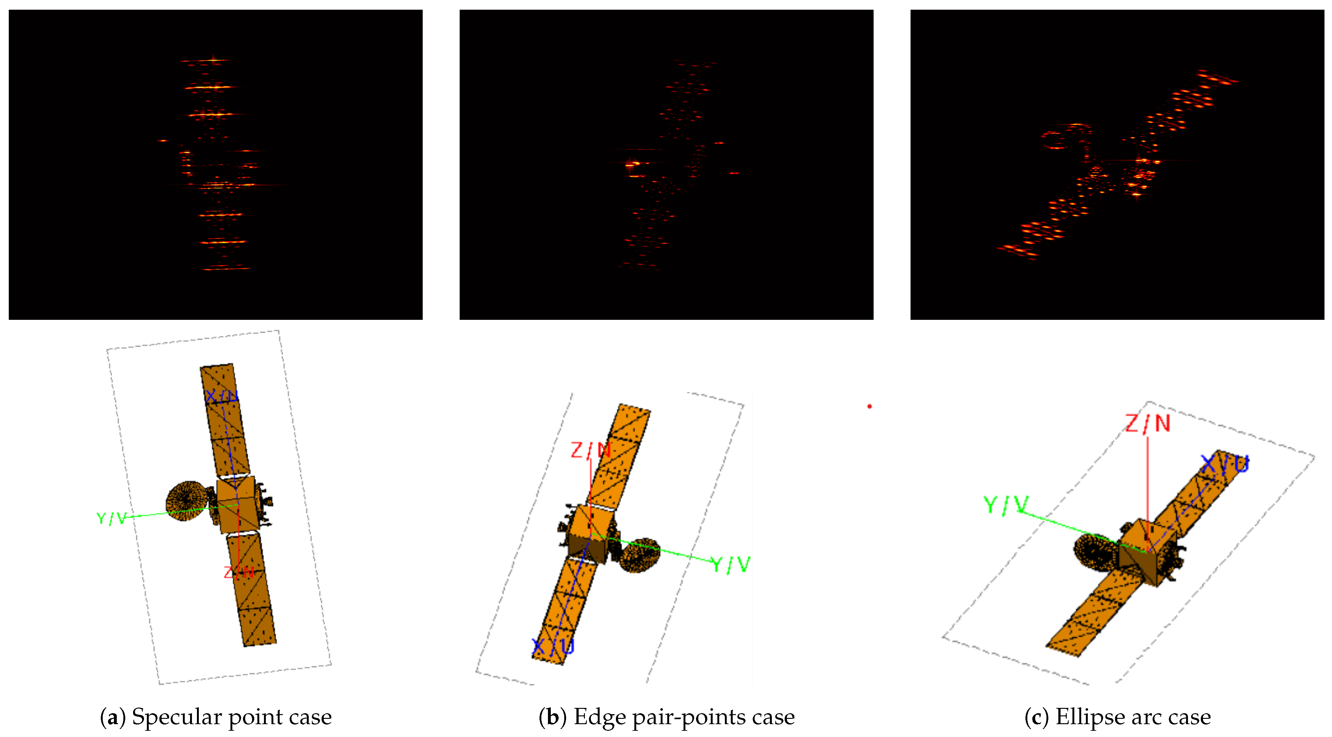
For the CAD (in the second row) and corresponding imaging characteristics (in the first row), we give three typical different apertures to observe, as shown in Figure 6. All observation apertures are with the same breadth, $3^{\circ }$, and the observing center angles $\phi$ are ${10}^{\circ }$, ${46}^{\circ }$, and ${70}^{\circ }$. From left to right, they are the three typical imaging characteristics, namely, specular point, edge pair-points, and ellipse arc, respectively. It can be found that the main body and solar panels are clearly discernible in all three observation apertures. In the case of the specular reflection point, as shown in Figure 6a, the parabolic antenna is not visible in the image; the specular scattering point occupies the majority of the energy, which is located at left to the satellite, and aligns with the analysis of component prior. In the case of the non-specular direction, there are two statuses of the parabolic antenna, corresponding to Figure 6b,c. It is easy to see that the parabolic antenna can be distinctly found in the image when it appears in the shape of an ellipse, which is shown in Figure 6c; and the parabolic antenna will be discretized into two endpoints when there are other strong scattering points in the observation aperture, as shown in Figure 6b. The readers can verify the position of the paraboloid by comparing the optical image with the corresponding viewing angle.

3. Improved Network for Component Detection

This study proposes a research framework for the automatic detection of satellite parabolic antenna components based on Inverse Synthetic Aperture Radar (ISAR) and deep learning. This section mainly develops a parabolic antenna component detection model based on the modified YOLOv8 algorithm, according to the features of the parabolic antenna analyzed in the previous section under terahertz radar imaging. Therefore, this section mainly introduces the basic structural framework of the proposed network, the relevant evaluation indicators, and the other algorithms involved in the comparison.

• A. Structure of Improved-YOLOv8 model

The most recent addition to the YOLO family of target detection algorithms, YOLOv8, boasts improvements across several key components over its earlier iterations. YOLOv8 incorporates an anchor mechanism inspired by YOLOX [30], which offers benefits in dealing with objects of elongated, unconventional shapes. Additionally, for the purpose of loss calculation in positive sample matching, YOLOv8 utilizes an adaptive multi-positive sample matching technique.

A variety of internal and external factors often result in size variations for satellites and their components, even in regions that appear identical. This diversity affects the size of the target detection area for the parabolic antenna. Yet, the target detection network generates detection boxes based on the fixed dimensions of a predefined box, which lacks flexibility. Further analysis of the samples in the dataset reveals that most samples have clear features and can be readily identified as simple samples. In contrast, a smaller number of samples have indistinct features, which raises the risk of misclassification, and are labeled as difficult samples. This creates a notable imbalance between simple and difficult samples. Nonetheless, it is essential for the model to be trained to recognize and differentiate these difficult samples so that the network’s detection capabilities can be improved.

Furthermore, the research introduces a refined algorithm derived from YOLOv8, designed for the automated detection of targets across multiple scales. Initially, a Dyhead [31] module, which employs an attention mechanism, is integrated into the algorithm’s head component to enable flexible detection of parabolic antenna targets that vary in size. Then, within the Intersection over Union (IoU) loss component, the standard Complete Intersection over Union (CIoU) from the YOLOv8 model is replaced with WIoU [32] to tackle the issue of sample imbalance between those that are easy to detect and those that are challenging. Figure 7 illustrates the primary architecture of the Enhanced-YOLOv8 algorithm.

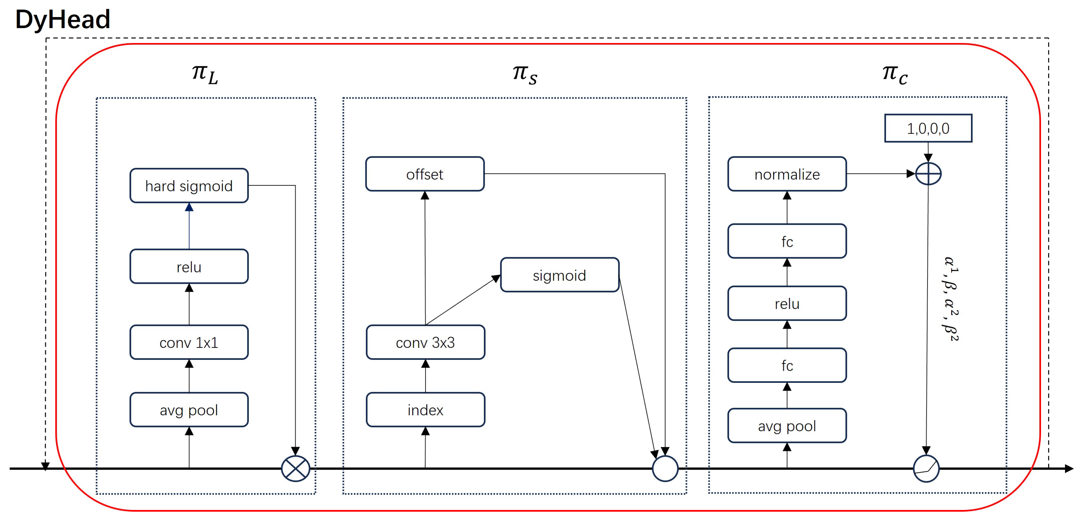
(1) Dyhead: The attention mechanism is a sophisticated processing strategy that prioritizes relevant information while excluding irrelevant, extraneous data. It adeptly captures the relative importance of various semantic levels and selectively boosts features in alignment with the dimensions of an individual object [31]. The Dyhead module integrates the target detection head and the attention mechanism together. This methodology seamlessly converges several self-attention components across different feature layers, spatial positions, and output channels, facilitating the concurrent acquisition of scale, spatial, and task awareness within a cohesive target detection architecture. This integration remarkably promotes the representational power of the detection head without augmenting the computational complexity. As illustrated in Figure 8, the detection head receives a scaled feature pyramid F, which is represented as a tensor $F\in R^{L\times S\times C}$, where L represents the number of layers within the pyramid. $S=H\times W$; H and W represent the height and width. And C denotes channel number of the median horizontal feature. The general procedure for utilizing self-attention can be expressed as:

$$W\left(\mathcal{F}\right)=\pi \left(\mathcal{F}\right)·\mathcal{F}$$

(21)

where $\pi (·)$ denotes an attention mechanism. A straightforward approach to addressing this attention mechanism involves the use of fully connected neural networks. However, training the attention function across all dimensions is computationally intensive and, in practice, not feasible due to the tensor’s high dimensionality. Alternatively, we decompose the attention function into three consecutive attentions, each dedicated to concentrating on a single perspective:

$$W\left(\mathcal{F}\right)={\pi }_C\left({\pi }_S\left({\pi }_L\left(\mathcal{F}\right)·\mathcal{F}\right)·\mathcal{F}\right)·\mathcal{F}$$

(22)

where ${\pi }_{L(·)}$, ${\pi }_{S(·)}$, and ${\pi }_{C(·)}$ represent three distinct attention functions, each applied to dimensions L, S, and C, respectively.

This module is equipped with scale-aware attention functions across the horizontal axis, and this module seamlessly integrates a range of different scales and thus effectively adjusts to the importance of various feature intensities. The scale-aware attention functions can be expressed as:

$${\pi }_L\left(\mathcal{F}\right)·\mathcal{F}=\sigma \left(f\left({\displaystyle \frac{1}{SC}}\sum _{S,C}\mathcal{F}\right)\right)·\mathcal{F}$$

(23)

where $f(·)$ denotes a linear function that is approximated through the use of a $1\times 1$ convolutional layer and $\sigma \left(x\right)$ is defined as the hard-sigmoid function given by $\sigma \left(x\right)=max(0,min(1,(x+1)/2\left)\right)$. The use of the hard-sigmoid operator is a key component of the attention mechanism, providing normalization, a probabilistic interpretation, and compatibility with the softmax function, all of which are essential for the effective operation of the attention mechanism in neural networks.

The spatially aware attention module operates within the spatial domain (specifically, along height and width), strategically pooling features from the same spatial locations across layers to yield more distinct feature representations, and can be expressed by

$${\pi }_S\left(\mathcal{F}\right)·\mathcal{F}={\displaystyle \frac{1}{L}}\sum _{l=1}^L\sum _{k=1}^K{w}_{l,k}·\mathcal{F}(l;p_k+\Delta p_k;c)·\Delta m_k,$$

(24)

where K represents the count of sparsely sampled positions, with $p_k+\Delta p_k$ indicating a relocated point achieved through the application of a spatial shift $\Delta p_k$ that the model has learned, which is designed to concentrate on a region of discriminative interest. Additionally, $\Delta m_k$ denotes a significance factor that the model has learned at the position $p_k$. Both of these elements are derived from the input features extracted at the median level of the feature set $\mathcal{F}$.

The task-specific attention module operates at the channel level, enabling the dynamic engagement or disengagement of operational channels to accommodate and support a variety of tasks, and can be expressed as

$${\pi }_C\left(\mathcal{F}\right)·\mathcal{F}=max\left({\alpha }^1\left(\mathcal{F}\right)·{\mathcal{F}}_c+{\beta }^1\left(\mathcal{F}\right),{\alpha }^2\left(\mathcal{F}\right)·{\mathcal{F}}_c+{\beta }^2\left(\mathcal{F}\right)\right)$$

(25)

where ${\mathcal{F}}_c$ denotes the feature tensor extracted from the c-th channel and the hyperparameter vector ${[{\alpha }^1,{\alpha }^2,{\beta }^1,{\beta }^2]}^T=\theta (·)$, which is determined by the function $\theta (·)$, is a specialized function that the model has been trained on to adjust activation thresholds. The function $\theta (·)$ is implemented in a manner akin to that described in reference [33], involving the following steps: first, it performs a global average pooling operation across the $L\times S$ dimensions to decrease the feature dimensionality, followed by two fully connected neural layers and a normalization layer. The output is then normalized using a shifted sigmoid activation function, constraining it to the range of $[-1,1]$.

(2) WIoU: In YOLOv8, the loss function is constructed from three distinct parts, which are divided into two unique streams, namely, classification and regression. For the former aspect, a Binary Cross-Entropy (BCE) loss is employed. For the latter aspect, the regression is handled using the CIoU bounding box loss and the Distribution Focus (DF) loss. A composite loss function is formulated by assigning appropriate weights to these three individual loss components, and it is represented as follows:

$${\mathrm{Loss}}^{\mathrm{total}}=u{\mathrm{Loss}}^{\mathrm{BCE}}+v{\mathrm{Loss}}^{\mathrm{DF}}+w{\mathrm{Loss}}^{\mathrm{CIoU}}$$

(26)

where, u, v, and w serve as weighting parameters.

The YOLOv8 implementation of the CIoU takes into account the overlapping region, the separation between the central points, as well as the shape ratio calculation within the bounding box regression procedure. Moreover, the way it defines the aspect ratio as a relative measure is not clear, and it fails to consider the equilibrium between difficult and simple sample types. WIoU addresses this by implementing a dynamic, non-increasing focus mechanism, which uses “outlierness” as a criterion for evaluating anchor box quality rather than IoU, and it also offers a well-considered approach to gradient distribution. As a result, WIoU is able to prioritize anchor boxes of average quality, thereby tackling the imbalance between challenging and easy samples and enhancing the detector’s overall effectiveness [32].

The WIoU is segmented into three distinct iterations: v1, v2, and v3, each characterized by its unique computational equations detailed as follows:

$$L_{\mathrm{WIoUv}1}=R_{\mathrm{WIoU}}\times L_{\mathrm{IoU}}$$

(27)

$$R_{\mathrm{WIoU}}=exp\left({\displaystyle \frac{{\left(x-x_{\mathrm{gt}}\right)}^2+{\left(y-y_{\mathrm{gt}}\right)}^2}{{\left({\mathit{H}}_g^2+{\mathit{W}}_g^2\right)}^{\ast }}}\right)$$

(28)

$$L_{\mathrm{WIoUv}2}=r\times L_{\mathrm{WIoUv}1},r={\left({\displaystyle \frac{L_{\mathrm{IoU}}^{\ast }}{{\overline{L}}_{\mathrm{IoU}}}}\right)}^{\gamma },\gamma >0$$

(29)

$$L_{\mathrm{WIoUv}3}=r\times L_{\mathrm{WIoUv}1},r={\displaystyle \frac{\beta }{\delta {\alpha }^{\beta -\delta }}}$$

(30)

$$\beta ={\displaystyle \frac{L_{\mathrm{IoU}}^{\ast }}{{\overline{L}}_{\mathrm{IoU}}}}\in (0,+\infty )$$

(31)

where $(x,y)$ and $(x_{gt},y_{gt})$ stand for the centroids of the anchor box and the ground-truth box, respectively. $W_g$ and $H_g$ refer to the measurements of the tightest surrounding rectangle. The presence of an asterisk (*) indicates that $W_g$ and $H_g$ are not part of the computational graph. $\beta$ measures the level of being an outlier, a parameter that is adjusted by the hyperparameters $\alpha$ and $\delta$. Moreover, r is used to denote the factor by which gradients are increased [32].

• B. Baseline Methods

The cutting-edge approaches in deep learning for target detection could be sorted into two main kinds: those that rely on region proposals and those that use regression. Region proposal-based methods, also referred to as two-step detection techniques, segment the detection process into two separate stages: the initial extraction of potential regions through algorithmic means, followed by a further refinement of these proposed bounding boxes. As a result, these methods tend to offer superior detection precision. Notable examples of such methods are the region-based Convolutional Neural Network (R-CNN) [34], FastR-CNN [35], and Faster R-CNN [36]. In contrast, regression-based methods, also known as one-stage detection techniques, dispense with the need for pre-selected regions. They are capable of identifying the target’s category and pinpointing its location in a single step, leading to rapid inference times. The YOLO series [37] and RetinaNet [38] are among the most prominent examples. This research endeavors to facilitate the swift and automated detection of subsidence funnels on extensive interferogram datasets. While two-stage methods are accurate, their intricate training processes and substantial computational demands pose challenges to real-time detection. Consequently, four exemplar one-stage detection methods were chosen for this investigation, YOLOv3 [39], YOLOv5 [40], YOLOv6 [41], YOLOv8 [22], and YOLOv11 [42], with the goal of enhancing the experimental workflow’s efficiency.

The YOLO (You Only Look Once) groups have emerged as a prominent family of object detection algorithms, with each iteration bringing significant advancements. YOLOv3, released in 2016, marked a milestone with its end-to-end architecture and ability to detect multiple objects simultaneously. Subsequently, YOLOv5, introduced in 2019, offered improved speed and accuracy with its more efficient design and multi-scale training approach. Building upon the success of YOLOv5, YOLOv6 introduced a novel backbone structure and data-efficient training strategies in 2021, aiming to find a middle ground between speed and precision. Then, YOLOv8 continued to push the boundaries with further enhancements in detection performance and efficiency, solidifying YOLO’s position as a leading algorithm within the realm of computer vision. Finally, YOLO11 is a cutting-edge, state-of-the-art object detection model, built upon previous versions of YOLO and incorporating new features and improvements to further enhance its performance and flexibility. Additionally, this study has opted for the lighter versions of the YOLO series models. In particular, YOLOv8 and YOLOv11 were chosen with the “n” variant, YOLOv5 and YOLOv6 were selected with the “s” variant, and YOLOv3 was chosen with the “tiny” variant.

4. Numerical and Anechoic Chamber Experiments

This section begins with an overview of the datasets and the specifics of the training process. Subsequently, a comparative evaluation of the detection performance across various networks is presented. Following this, the results of ablation studies focused on quantitative assessments and the impact of network components are discussed. Furthermore, experiments conducted in anechoic chambers are performed to demonstrate the superiority of robustness when compared to other networks.

• A. Dataset construction and experimental details

The method is verified by electromagnetic calculation data and an anechoic chamber. The simulation data are constructed and supported by the electromagnetic simulation software and satellite CAD model. The imaging parameters are configured to the following specifications: the center frequency is 220 GHz, the bandwidth is 20 GHz, the number of sampling points is 1200; the azimuth aperture is $3^{\circ }$ with 500 points for sampling. The depression angle is set as ${45}^{\circ }$. Taking into account the imaging resemblance between neighboring observation apertures, a set of 617 original images is acquired by selecting them at a $0.{58}^{\circ }$ interval from a total of ${360}^{\circ }$. 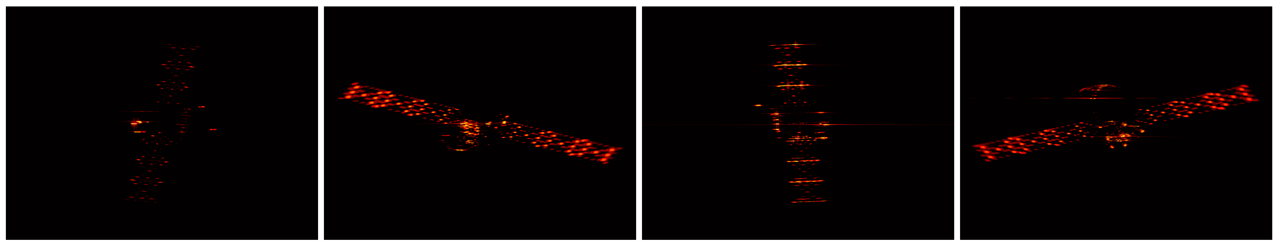Figure 9 demonstrates various representative imaging outcomes across a range of observation apertures.

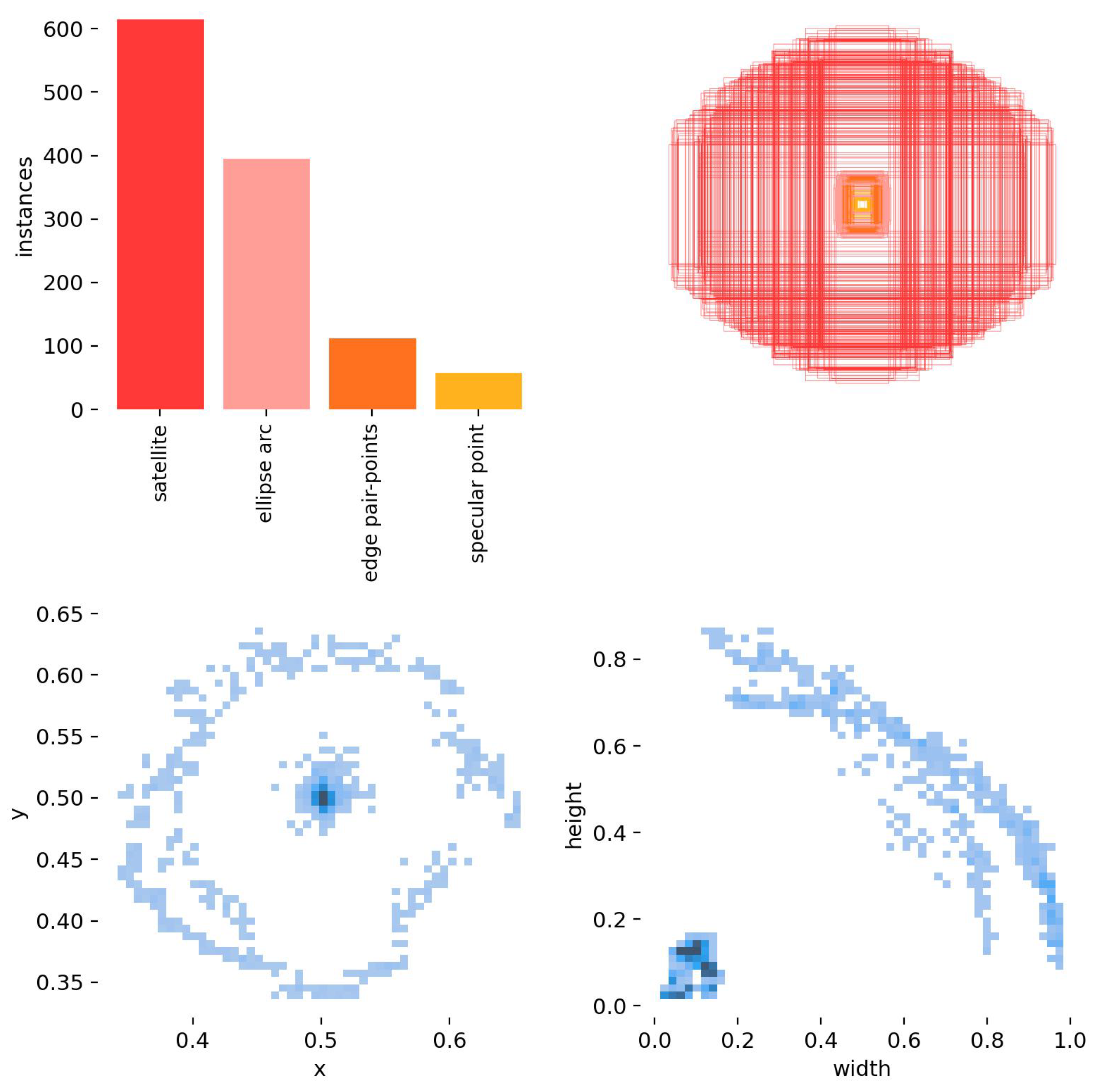
Next, we need to label the target for detection based on CPICs. Provided that the primary components of the satellite and parabolic antenna are discernible in the image, they are marked or labeled. Furthermore, the difference in the bounding boxes of the satellite and the antenna is illustrated in Figure 10. We can see that the bounding boxes of the satellite are significantly larger than the three kinds of bounding boxes for the parabolic antenna, particularly the bounding box for the specular point, which tests the multi-scale detection capability of the object detection network. Additionally, the distribution of the three bounding boxes for the parabolic antenna is uneven. Among them, there are approximately 400 types of ellipse arc, 100 types of edge pair-points, and around 50 types of specular point. The total number of ellipse arc and edge pair-points accounts for nearly $90\%$, and together they form the main part of the antenna.

The mean Average Precision (mAP) serves as a crucial measurement for assessing the performance of deep learning models. It is of paramount importance due to its ability to provide a comprehensive evaluation of accuracy and recall capabilities across various trained instances. The choice of mAP as an evaluation criterion is justified because it is extensively utilized in numerous object detection research studies, offering a standardized and reliable way to compare the effectiveness of different models in identifying and recalling objects accurately. We choose mAP50 and mAP50-95 to evaluate the training results. The mAP50 metric measures the average precision of the model when the IoU (Intersection over Union) threshold is set to 0.5, while mAP50-95 measures the average precision of the model over the IoU threshold range from 0.5 to 0.95. 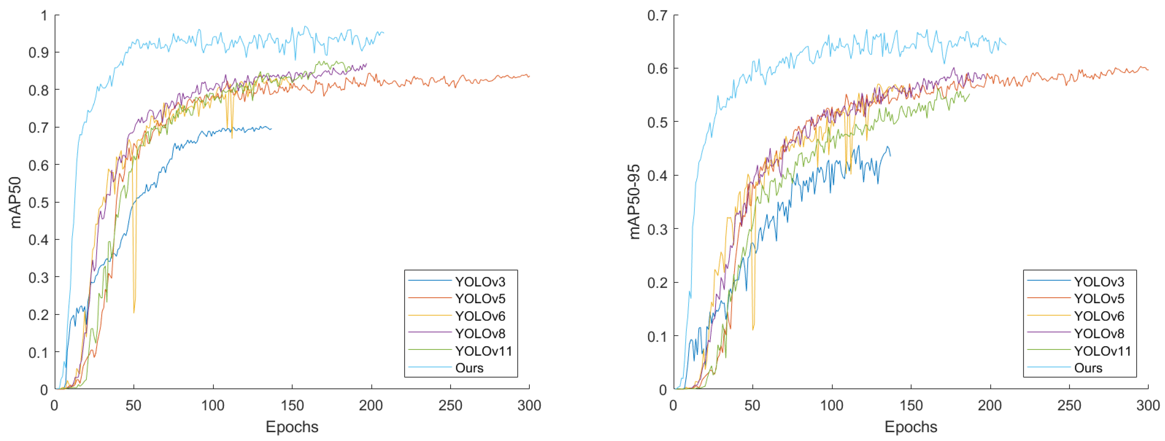Figure 11 shows the changes in mAP during the training process for different networks. The left side of Figure 11 shows that the training results of YOLOv3 are poor, and the training was terminated before reaching 0.7; YOLOv8 has an mAP50 around 0.8, which is a little better training effect than in YOLOv5 and YOLOv6. The proposed methods both have mAP50 values exceeding 0.9, maintaining a high level of training. The right side of Figure 11 gives the comparison result of mAP50-95. It shows that apart from the overall numbers having decreased by about 0.3, the overall trend remains unchanged. To further highlight the recognition superiority of the proposed method for parabolic antenna components, the next section will focus on analyzing the performance indicators of different algorithms for parabolic antenna detection. Moreover, the relevant parameters are $epochs=300$ and $patience=50$, which means the program will stop when the number of epochs reaches 300, or when there is no significant improvement over a continuous 50 iterations. So, we can see that different algorithms vary the epochs in Figure 11.

Taking into account the visual proximity among neighboring observation apertures, a selection of 620 pristine images is compiled by spacing them at intervals of 0.58 degrees within a full 360-degree range, as suggested in [26]. The dataset is segmented into training, validation, and testing subsets, with allocations of $70\%$, $10\%$, and $20\%$ each for these respective phases. To enrich the variety of the training images, conventional data augmentation techniques such as horizontal mirroring, brightness adjustment, and the introduction of random noise are employed. To improve the model’s generalization ability, mosaic enhancement is applied to each image; to reduce computational load, the image size is reduced to 0.5 times the original size; the image brightness will be adjusted to about 0.4 of the original brightness; there is a 0.5 probability of horizontally flipping the input image during each random training sample generation. All the experiments were conducted on a system featuring an Intel(R) Core(TM) i9-13900HX processor running at 2.20 GHz, complemented by an NVIDIA GeForce RTX 4060 graphics card. The PyTorch deep learning library, specifically the GPU-enabled version, was utilized as the primary framework for these experiments. CUDA 11.8 was employed for the parallel processing capabilities of the GPU. The SGD optimizer was chosen for updating and optimizing the network parameters. The initial training learning rate was initialized to 1 × 10⁻³. The mini-batch size was specified as 32, and the total number of training epochs was set to 300. The input image size was 640, the number of worker threads for data loading was 8.

• B. Accuracy Verification

To assess the effectiveness of deep learning models, the primary measure employed is the mean Average Precision (mAP). This measure is commonly applied in object detection research to depict the accuracy and recall patterns across different trained models [43]. The AP is computed through the difference-based AP evaluation technique, which represents the region below the precision–recall curve. The calculation formula is:

$$\mathrm{AP}=\left({\displaystyle \frac{1}{n}}\sum _{\left(rϵ{\displaystyle \frac{1}{n}},{\displaystyle \frac{2}{n}},...,{\displaystyle \frac{n-1}{n}},1\right)}{P}_{\left(r\right)}\right)$$

(32)

$$\mathrm{mAP}={\displaystyle \frac{1}{N}}\sum _{k=1}^{k=N}{\mathrm{AP}}_k$$

(33)

where n means the entire number of detection instances. $P\left(r\right)$ signifies the accuracy level at a specific recall rate of r. N refers to the complete count of categories, and $A{P}_k$ denotes the AP for category k. $mA{P}_{50}$ refers to IoU thresholds set at $50\%$. And mAP is short for $mA{P}_{50}$ in this paper in the absence of ambiguity. Furthermore, auxiliary assessment metrics such as precision, recall, and the F1 measure are represented mathematically in the following manner:

$$\mathrm{Precision}={\displaystyle \frac{\mathrm{TP}}{\mathrm{TP}+\mathrm{FP}}}$$

(34)

$$\mathrm{Recall}={\displaystyle \frac{\mathrm{TP}}{\mathrm{TP}+\mathrm{FN}}}$$

(35)

$$F1=2·{\displaystyle \frac{\mathrm{Precision}·\mathrm{Recall}}{\mathrm{Precision}+\mathrm{Recall}}}$$

(36)

where TP stands for true positives, indicating the case where an object is accurately identified as a positive example. FP denotes false positives, involving the erroneous identification of an object that is not actually positive. FN refers to false negatives, where a legitimate object is mistakenly classified as negative.

• C. Comparisons with other algorithms

To evaluate the detection performance fairly, the following representative algorithms are chosen for comparison: YOLOv3, YOLOv5, YOLOv6, YOLOv8 and YOLOv11.

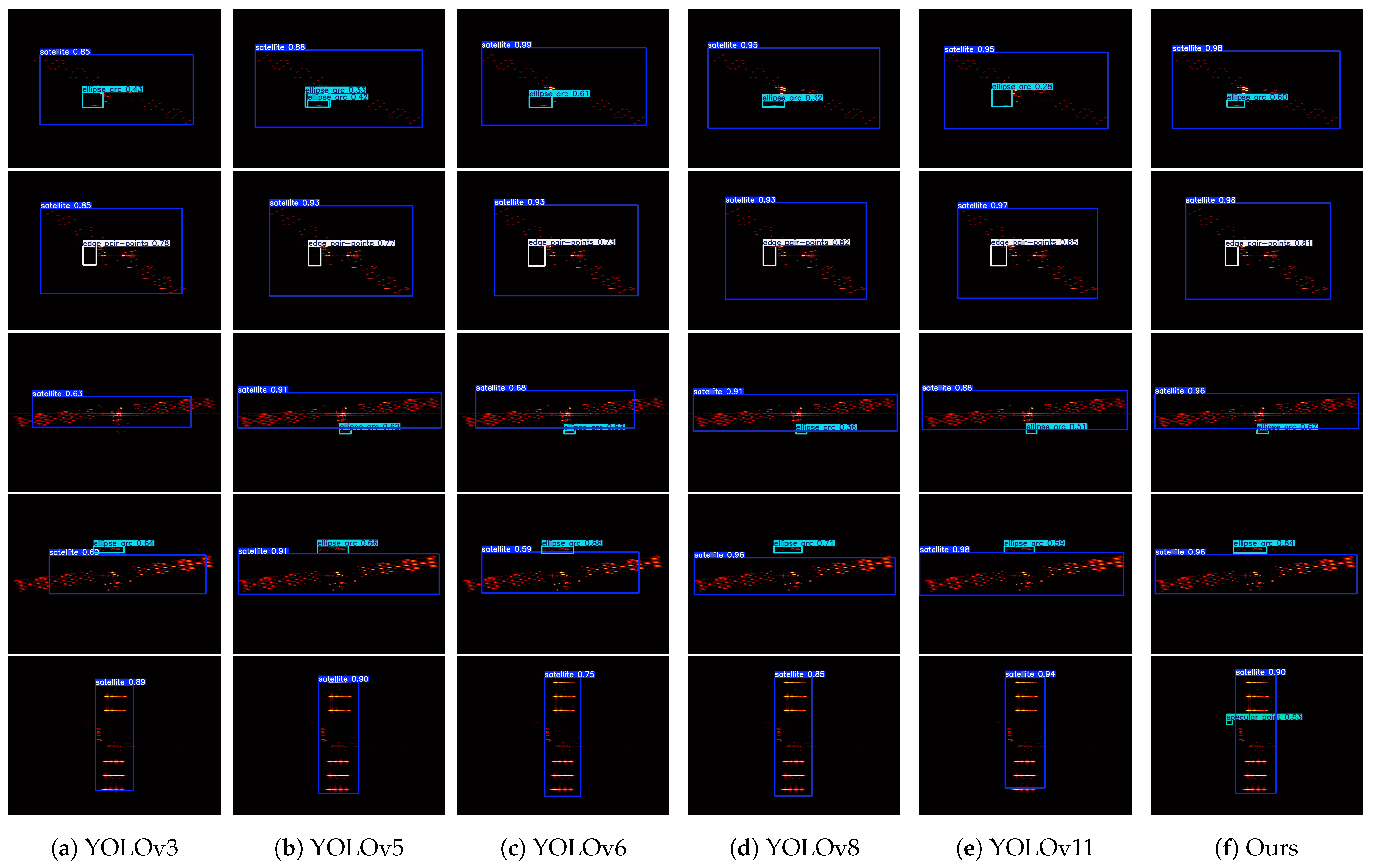
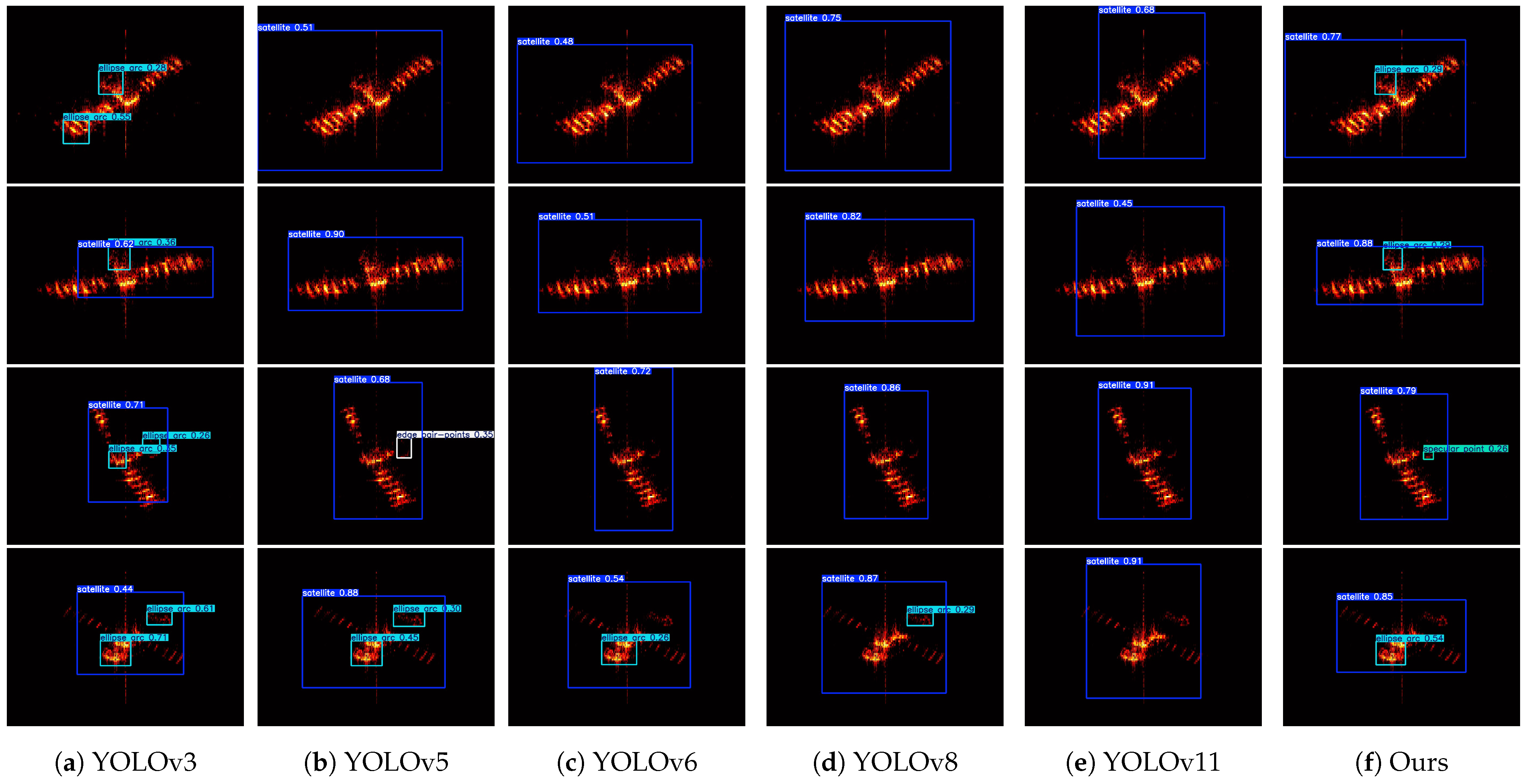
Figure 12 presents the outcomes of detecting objects using seven various detection networks. The images across each row illustrate the detection results from these networks at a set focal width. The boxes marked in red, pink, orange, and yellow indicate the identified areas of the satellite, the ellipse arc, the edge pair-points, and specular point, respectively. Observations reveal that ours successfully detects the parabolic antenna and satellite for all five samples, while others have varying degrees of shortcomings. YOLOv3, YOLOv5, YOLOv6, YOLOv8, and YOLOv11 miss the detection of the component in row 5, which indicates our network’s advantage in recognizing small-scale targets. Meanwhile, YOLOv3 misses detection in row 3, and the identification outcomes of YOLOv5 yield numerous intersecting bounding boxes for the elliptical arc, suggesting that the network necessitates a more refined Non-Maximum Suppression (NMS) threshold.

Table 2. The performance metrics across various networks in the context of satellite analysis.

Networks	P	R	F1	mAP50	mAP50-95
YOLOv3	0.968	1	0.984	0.994	0.679
YOLOv5	0.996	1	0.998	0.995	0.871
YOLOv6	1	0.98	0.99	0.995	0.766
YOLOv8	0.986	1	0.993	0.995	0.824
YOLOv11	0.996	0.989	0.981	0.994	0.794
Ours	0.996	1	0.998	0.995	0.873

,

Table 3. The performance metrics across various networks in the context of specular point analysis.

Networks	P	R	F1	mAP50	mAP50-95
YOLOv3	0.484	0.054	0.097	0.054	0.010
YOLOv5	0.991	0.333	0.498	0.628	0.217
YOLOv6	0.924	0.222	0.358	0.336	0.153
YOLOv8	0.756	0.278	0.407	0.352	0.123
YOLOv11	0.799	0.333	0.470	0.442	0.148
Ours	0.793	0.778	0.785	0.838	0.283

,

Table 4. The performance metrics across various networks in the context of edge pair-points analysis.

Networks	P	R	F1	mAP50	mAP50-95
YOLOv3	0.67	0.905	0.770	0.913	0.566
YOLOv5	0.736	0.952	0.830	0.913	0.627
YOLOv6	0.653	0.895	0.755	0.891	0.581
YOLOv8	0.694	0.952	0.803	0.933	0.62
YOLOv11	0.624	0.857	0.722	0.852	0.536
Ours	0.902	0.948	0.924	0.989	0.685

and

Table 5. The performance metrics across various networks in the context of ellipse arc analysis.

Networks	P	R	F1	mAP50	mAP50-95
YOLOv3	0.93	0.784	0.851	0.851	0.518
YOLOv5	0.902	0.94	0.921	0.96	0.593
YOLOv6	0.862	0.957	0.907	0.947	0.585
YOLOv8	0.856	0.897	0.876	0.943	0.59
YOLOv11	0.894	0.897	0.876	0.917	0.541
Ours	0.889	0.948	0.918	0.978	0.591

present performance metrics across various networks in the context of the satellite, the ellipse arc, the edge pair-points, and specular point quantitatively. From Table 2, we can tell that all networks detect the satellite accurately, which demonstrates stability in large target detection. Observing Table 3, it can be found that ours achieves the highest F1, R, mAP50, and mAP50-95, and the highest score of P is achieved by YOLOv5. In Table 4, we can see that the proposed algorithm achieves the top values across P, F1, mAP50, and mAP50-95 metrics, with YOLOv8 and YOLOv5 holding the top position for the R metric. In Table 5, the proposed algorithm also exhibits the highest mAP50 value, while YOLOv3 and YOLOv6, respectively, claim the top spots for the P and R metrics and YOLOv5 holds the top spots for the F1 and mAP50-95 metrics.

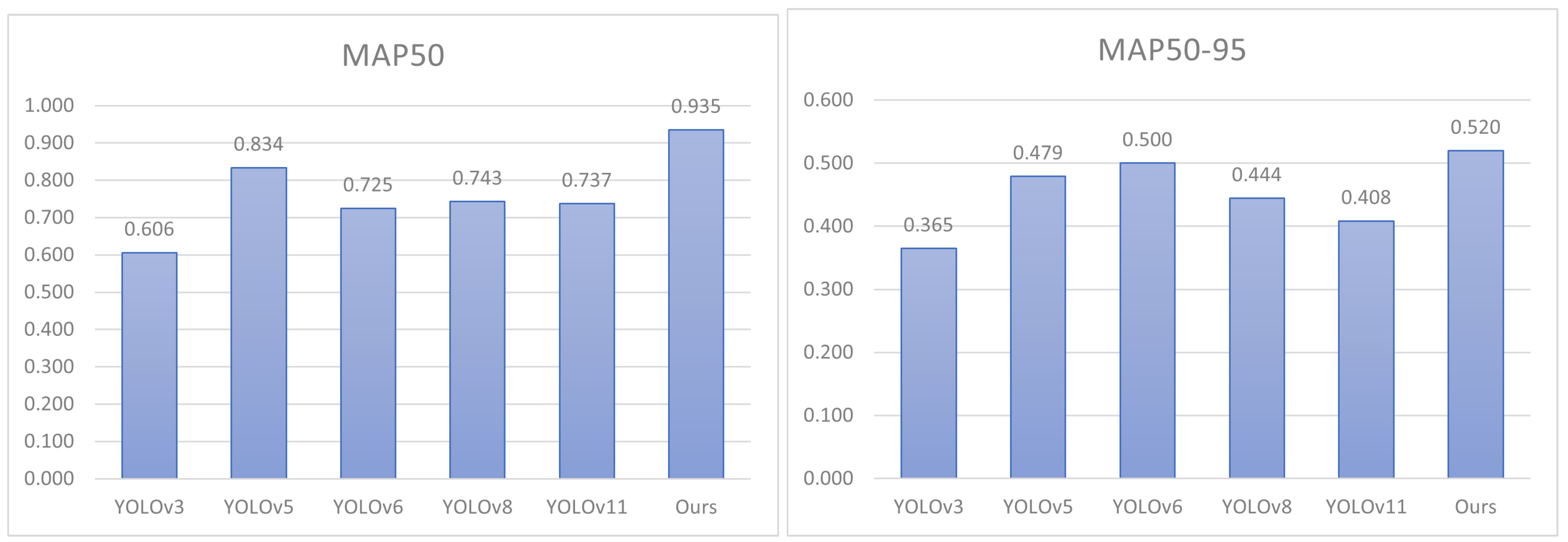
In order to focus attention on the detection of parabolic dish antennas, by integrating the mAP50 and mAP50-95 values from the aforementioned tables, namely, Table 3, Table 4 and Table 5, we obtain the following histogram in Figure 13. As a result, the efficacy of the suggested approach achieves peak levels in the recognition outcomes for parabolic antenna.

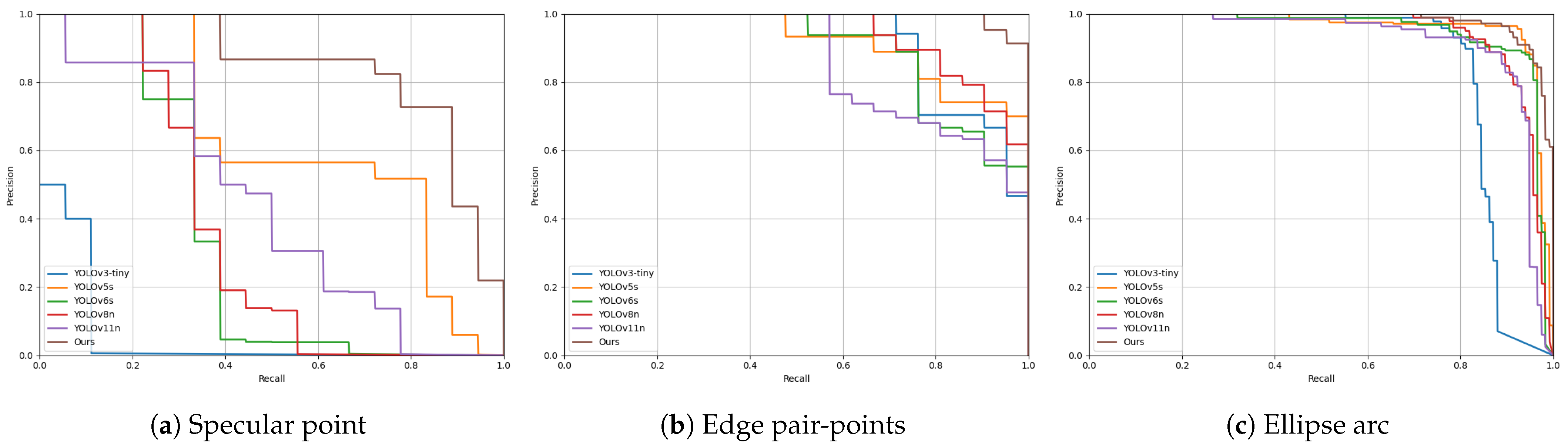
In order to gain a more detailed assessment of the detection capabilities, the precision–recall (PR) curves of the ellipse arc, the edge pair-points, and specular point are presented in Figure 14. For the ellipse arc, the proposed algorithm’s advantage is not significant. But for the specular point and edge pair-points, our algorithm is situated in the upper right-hand side of all the curves, thus verifying the stability of the detection.

To illustrate the improvement effects of the combined enhancement module, namely, Dyhead + WIoU (DW), introduced in this paper on the YOLOv8 model, and to further compare the impact of different versions of WIoU, we conducted ablation experiments on the Improved-YOLOv8 model. Considering the conservation of computational resources, we only chose to add one Dyhead module. Additionally, there exist three variations of WIoU: v1, v2, and v3, among which WIoUv3 requires the determination of hyperparameters $\gamma$ and $\delta$ [32] with the classic values $\gamma =1.9$ and $\delta =3$. We show the results of mAP as an index to assess the performance of the proposed network quantitatively. The findings are presented in

Table 6. Ablation experiment.

Method	MAP(%)
YOLOv8	0.743
YOLOv8 + WIoUv3	0.808
YOLOv8 + WIoUv2	0.737
YOLOv8 + WIoUv1	0.917
YOLOv8 + Dyhead	0.906
YOLOv8 + Dyhead + WIoUv3	0.859
YOLOv8 + Dyhead + WIoUv2	0.926
YOLOv8 + Dyhead + WIoUv1	0.935

.

Table 6 visually illustrates the changes in model accuracy after adding Dyhead and different versions of WIoU. According to the aforementioned results, we could sum up that when the two modules are combined, i.e., Dyhead + WIoUv1, there is a significant improvement in model performance. As previously described, the Dyhead module helps the network to adaptively detect various scales of parabolic shapes from ISAR images, while WIoU to some degree mitigates the problem of sample unevenness between simple and complex examples.

• D. Recognition Performance in Anechoic Chamber Measurement Data

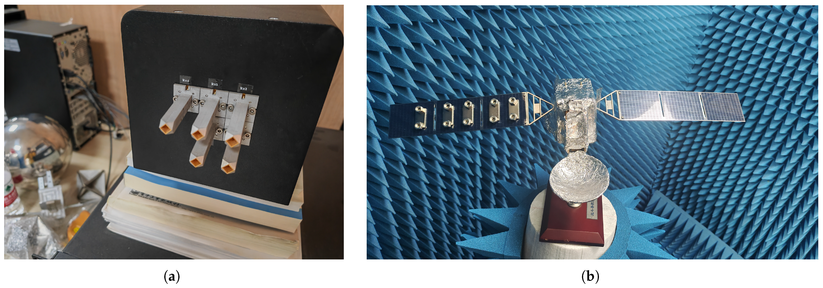
Figure 15 illustrates the configuration of an anechoic chamber and presents a photograph of the satellite prototype. The radar transmits a linear frequency-modulated signal. Its start frequency and end frequency are 324 GHz and 344 GHz, respectively. This is a terahertz radar system with one transmitting antenna and four receiving antennas. For this experiment, only one of the receiving channels was used. In addition, a satellite model with a length of approximately 70 cm was mounted on an accurately calibrated turntable for capturing images through various observation apertures.

Figure 16 shows the recognition outcomes of different algorithms for the four anechoic chambers’ measurement data. From the figure, we can see that YOLOv3 has poor performance with misrecognition for both satellites and parabolic antenna; and YOLOv11 recognizes all the satellites but misses all parabolic antennas; YOLOv5 loses the recognition of two parabolic antennas and also duplicates the recognition of parabolic antennas; YOLOv6 and YOLOv8 lose the recognition of three parabolic antennas, and the latter has a false recognition, showing a weak generalizability. The proposed algorithm is able to recognize both satellites and parabolic antennas without any omissions or misjudgments, which fully demonstrates that the addition of modules can adaptively detect various scales and can solve the issue of sample imbalance between different types of samples.

• E. The limitations of the Improved-YOLOv8

Although the proposed algorithm performs well on electromagnetic simulation datasets and can correctly identify some dark room data, exceeding most YOLO models and to some extent demonstrating the algorithm’s superiority, it has not been compared with other one-stage or two-stage models. In the design phase of the algorithm, we mainly focused on data processing under ideal conditions. While it can successfully identify some dark room measurement data, it has not yet conducted in-depth analysis and optimization for the noise interference that may be encountered in practical applications. Moreover, this paper has fully analyzed the imaging characteristics of smooth parabolic antennas under non-polarized conditions and achieved good recognition results. However, the study has not explored other types of parabolic antennas, such as those equipped with feed sources or with grid-shaped parabolic antennas; therefore, it cannot be guaranteed that the generalizability to other structures of parabolic antennas remains. In addition, the improved-YOLOv8 model proposed in this study mainly optimizes the final detection process of the model by modifying the head part, thereby improving the model’s performance. However, since the model has not been improved in the backbone and neck parts, it has not further optimized the model’s feature extraction and enhancement process. Therefore, in the future, we will focus on enhancing the model’s multi-scale feature extraction capabilities.

5. Conclusions

In summary, this article proposes an algorithm based on component prior knowledge and an improved version of YOLOv8, which achieves the identification of parabolic antennas on satellites. With reference to the specified imaging geometry and standard imaging techniques, the CPICs of the parabolic antenna in the THz band were analyzed, and the corresponding dataset was established. By effectively using the special CPICs, we transformed this component identification problem into three different types of object detection problems. Subsequently, by incorporating Dyhead and WIoU, the multi-scale target challenges and sample imbalance in the satellite ISAR images were addressed. Trained on simulated data, the Improved-YOLOv8 model achieved 0.935 and 0.52 in AP50 and AP50-95, respectively, surpassing the baseline YOLOv8 model. Compared with five other detection algorithms, YOLOv3, YOLOv5, YOLOv6, YOLOv8, and YOLOv11, our method notably improved about by 0.33, 0.10, 0.21, 0.19, and 0.20 in mAP50 and improved by about 0.16, 0.04, 0.02, 0.08, and 0.11 in mAP50-95. And for the anechoic chamber measurement data, the effectiveness and reliability of the proposed method in identifying parabolic antennas were also verified.

Recognizing the parabolic antenna, which is a major component of satellite communication systems on satellites in space, possesses immense application potential. It plays a significant role in ensuring the success of satellite missions and maintaining satellite’s safety and repair. In the future, we will consider this method to apply to other types of satellites as well as the detection of parabolic antennas and recognition under low signal-to-noise ratios. And the discussion about the improvement of the backbone of the network and different training strategies will be taken into account.