Abstract
A key component of the new stochastic approach for discontinuity shear strength (referred to as StADSS) is characterising the roughness of natural rock discontinuities at full scale to mitigate well-known scale effects on shear strength predictions. An investigation was conducted using the software Blender (v4.0) to determine the influence of camera orientation and position on the estimation of the standard deviation of gradients, a parameter used to quantify roughness and to make predictions of discontinuity shear strength. The existing literature has investigated the various distortions of images due to camera position and orientation; however, a comprehensive understanding of their unique influence on error in shear strength prediction is still missing. The investigation revealed that a ground sampling distance of less than 1.36 mm/pixel allows the standard deviation of gradients to be quantified within approximately ±10% relative error to the control data set. Based on investigations into camera orientation relative to the planar control data set, error on the roughness parameter due to perspective distortion was quantified. Recommendations were made to reduce perspective distortions and improve seed trace digitisation errors, including capturing images perpendicular to the seed trace with no rotation and getting as close as possible to the trace during capture to improve ground sampling distance. Lastly, the influence of these different trace digitisation errors on predictions of shear strength obtained using StADSS was investigated. Digitisation errors were found to have a disproportionate influence on shear strength prediction error, especially for rough discontinuities at low normal stress. The investigation highlighted the importance of accurately digitising the standard deviation of gradients to predict discontinuity shear strength.
1. Introduction
The recent growth of critical infrastructure, including open pit mines, tunnels, road cuttings, and other deep excavations, combined with increasing financial and environmental constraints, puts pressure on engineering designs to be less conservative. One source of such conservatism lies in the estimation of shear strength for large rock discontinuities, which contributes to the stability of rock masses [1]. Until recently, the prediction of discontinuity shear strength has been subject to scale effects [2,3,4,5,6,7,8,9,10,11,12,13,14], often resulting in overly conservative design. Despite decades of research into roughness and scale effects on discontinuity shear strength, there remains no consensus on how to reliably predict discontinuity shear strength at large scale [15].
There are many shear strength models that recognise different properties of discontinuities contributing to shear strength such as roughness [5,16,17,18,19,20,21], infilling [22,23,24,25,26,27,28], anisotropy [29,30,31], persistence [32,33,34], and mismatch or aperture [35,36]. However, most shear strength models are primarily based on roughness. Arguably, the current industry standard for shear strength prediction is Barton and Choubey’s empirical joint roughness coefficient (JRC) method [5]. The revised JRC model [2] accounts for scale dependent parameters, though concerns remain to its formulation and methodology [17,18,37]. Also, the scale effects on roughness were not clearly understood and only were accounted for based on an empirical chart comparing trace length and amplitude [2]. The roughness of discontinuities is difficult to quantify due to being multiscale and often non-stationary [38]. An additional challenge comes from the fact that discontinuity surfaces are usually contained within the rock mass, preventing their complete 3D roughness characterisation. Often, the only roughness datum available is the 2D profile of the discontinuity exposed on the rock face, usually referred to as a trace.
A stochastic approach for discontinuity shear strength (referred to as StADSS) was proposed by Buzzi and co-workers [20,21,38,39,40,41,42]. This novel approach predicts the peak and residual shear strength of rough rock discontinuities at full scale whilst by-passing the well-known scale effects on roughness [2,3,4,5,6,7,8,9,10,11,12,13,14]. Roughness is quantified through a multiscale statistical analysis of an exposed, daylighting seed trace at full scale, referred to as a seed trace [38]. A random field model (RFM) generates several synthetic surfaces which share the same statistical characteristics as the seed trace. Rock strength parameters and the generated synthetic surfaces are the input to a deterministic shear strength model, used to conduct a series of Monte Carlo simulations. The Newcastle discontinuity shear strength (NDSS) model [20,21] is used within StADSS to deliver a statistical distribution of peak and residual shear strengths which can be used in stability analysis. StADSS has been shown to closely predict the peak and residual shear strength of prepared specimens replicating natural joints [20,21]; more recently, it was applied to a large in situ specimen [43].
The seed trace of a discontinuity must be accurately digitised to allow for the application of StADSS. Roughness information can be obtained from contact and non-contact approaches. In the rock mechanics field, many would be familiar with the mechanical profile comb used to characterise roughness at small increments [5,30]. This method was found to be subjective and unreliable due to human error [17,18,37] and is also only applicable to small lengths (commonly 100 mm). All contact methods including the profile comb also require physical access to the rough rock surface, which is often not possible when the discontinuity is contained within the rock mass. Lastly, when applying a shear strength model, physically accessing the surface/discontinuity may not be safe or possible, making seed trace digitisation by contact an invalid approach. Non-contact approaches to digitise roughness have also been investigated, including photogrammetry [44,45,46], and laser scanning [10,47,48]. However, a seed trace is often only identifiable by its contrast in colour from the remainder of the rock mass. Discontinuities that are tight and unweathered may exhibit insufficient data to allow for digitisation by laser scanning or photogrammetry. To avoid the need to physically access a seed trace, a non-contact approach must be developed to allow application of StADSS to common discontinuities in the field where physical access is not possible or safe. The most promising non-contact approach applicable to the development of StADSS is by processing images [49,50]. Images have many advantages over other methods:
High-resolution images can be captured using hand-held digital cameras or with drones enabling remote access to potentially unsafe and difficult to reach areas.
High-quality cameras (both hand-held and mounted to drones) are now relatively affordable and cost-effective items used in industry.
Images capture a lot of data, including the colour and relative positions of objects within the image. A combination of information ideal for digitising seed traces in the field.
It is for these reasons that high-resolution images were pursued as the proposed approach to digitise seed traces for application of StADSS to natural rock discontinuities. Essentially, the digitisation methodology comprises capturing a high-resolution image of the seed trace, extracting the profile of the trace during processing, and scaling the data using survey data from the site.
Given the importance of trace roughness information for the prediction of shear strength [45,51], it is essential for the seed trace to be digitised at high resolution and with an effort to reduce errors. Capturing the profile of a natural trace in the field with high accuracy can be challenging because of limited access, size of the discontinuity and trace, weather, and lighting conditions.
The orientation of a camera relative to an object (in this case, a seed trace) is important to ensure the objects captured within the image are least affected by perspective distortion. Ideally, the camera should be oriented perpendicular in all directions to the object dimensions desired to be proportionally correct within the image. This orientation reduces the effects of pose, distance, and foreshortening [52]. Whilst corrective models for perspective distortion do exist [52,53,54,55], these will not be investigated within this process for simplicity and because they become complex when applied to irregular 3D scenes such as rock faces [56].
This paper presents the results of a study on the quantification of errors on a discontinuity roughness descriptor resulting from camera rotations around two axes and photograph resolution. Poor information capture will result in errors on the estimation of roughness, which, in turn, will result in error in shear strength predictions. Although the significance of ground sampling distance and image distortion have been extensively studied in other applications, there is no information in the literature on those effects on the quantification of roughness for large in situ discontinuities. As far as the authors know, there are no published data on identifying the influence of camera position (distance, and orientation) on the relative error of standard deviation of gradients, a roughness indicator, and its effect on predictions of shear strength for rough rock discontinuities. Hence, the novelty of this investigation lies in determining the magnitude of the influence of different image distortion errors and systematic errors in the trace extraction methodology on predictions of shear strength using a recently developed shear strength prediction approach named StADSS [45].
2. Methodology
The seed trace digitisation methodology comprises a sequence of steps beginning with the capture of the images on site followed by post-processing:
- Capture a high-resolution image containing the entire seed trace and take survey measurements (tape measure, ruler, or theodolite survey) on site for scale.
- Trace the profile of the seed trace in the image at single pixel increments manually or using a customised Python script. The rock mass and seed trace should be coloured white and black, respectively, to increase the contrast between intact rock and discontinuity trace.
- Extract the coordinates of the seed trace profile within the image at single-pixel increments. Depending on the trace thickness, a top and bottom trace can be extracted at each pixel position on the horizontal axis. In this investigation, only the top trace was extracted.
- Scale the seed trace data using the physical measurements taken on site. This converts the trace coordinates from pixels to millimetres using linear interpolation.
Examples of steps 1, 2, and 3 are illustrated in Figure 1 [57].
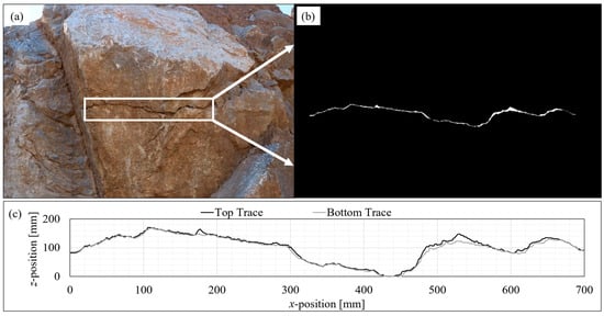
Figure 1.
(a) Photograph showing the full length of a seed trace exposed on a natural rock face. The white box indicates the border of the trace which has been converted to a binary image in part b of this figure. (b) Binary-coloured image depicting the profile of the seed trace in white and the remainder of the rock mass in black. The trace is separated from the remainder of the rock mass using a binary colouring system to simplify extracting the coordinates of the white pixels. (c) The extracted height coordinates of the top and bottom seed traces taken from part b of this figure [57].
The coordinates of the trace profile are extracted using a top–down approach. A Python script starts the identification in the top left pixel of the image; if this pixel is coloured as rock mass, it then moves down a single pixel and repeats this process. If the next pixel is coloured as seed trace, the script identifies this as the coordinate of the top trace for that column of pixels. Extracting the coordinates of the bottom trace is not applicable within this paper. The script then progresses to the next column of pixels and repeats the process. This is demonstrated visually in Figure 2.
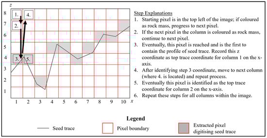
Figure 2.
Illustration of the process followed to identify the top trace coordinates of a seed trace. This presents a simplified version where the thickness of the trace profile is a single line, and the resolution of the image is low. Each numbered cell from 1 to 5 within the array presents a step described on the right of the figure.
The main sources of errors when digitising the trace are expected to come from steps 1 and 2. This paper aims to quantify the errors encountered primarily during step 1 of the digitisation methodology by investigating the influence of the camera’s distance from the trace and the orientations of the camera relative to the trace. Some errors are also expected to occur during post-processing due to image types, data compression, and geometric anomalies caused by digitising roughness at pixel increments. This paper does not address errors due to survey accuracy on site used to scale the trace data, edge detection of the trace in photographs of real rock surfaces, or errors due to methods used to digitise very long traces not containable within a single image. These issues will be addressed in further research. To quantify the desired errors, the following steps shown in Figure 3 will be followed, and the following sections provide specific information on each step of the methodology.
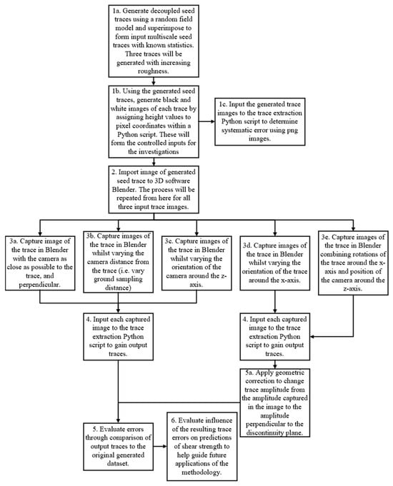
Figure 3.
Flow chart of the methodology followed in this study to quantify different digitisation errors.
2.1. Random Field Model and Control Trace Generation
Control traces with known roughness statistics were generated using a multiscale Gaussian random field model. The control traces were generated to simulate real in situ traces because the roughness statistics of real in situ traces are unknown. The simulation of the traces in a 3D software is explained in Section 2.2. Three control traces of increasing roughness were generated. They were 5 m in length and characterised by their standard deviation of gradients (sdi), which was 0.31 m/m, 0.71 m/m, and 1.12 m/m, respectively. More information on the input traces is found in Table 1. The trace length of 5 m was nominally adopted to cover situations the authors believed most likely to encounter in the field where StADSS or CFR would be required to gain predictions of shear strength of a natural rock discontinuity.

Table 1.
Summary of roughness characteristics (from left to right, including standard deviation of gradients, mean of heights, standard deviation of heights, and mean of gradients) of the input multiscale seed traces generated by the random field model.
The random field model was written using components of the GSTools (v1.5.0) random field modelling package in Python [58], with a Gaussian covariance model for spatial correlation. The GSTools (v1.5.0) package provides the framework to write unique random field models for specific tasks; in this case, a model was written to generate 2D seed trace data with known output statistics and inputs. The inputs to the random field model are the mean and variance of asperity height, the dimension of the field created (5001 points for a trace 5000 mm long), and the correlation length. These values were based off decoupled trace data [21] but were altered through trial and error to achieve the desired statistics of each trace.
Each trace was obtained by superposing three daughter traces with different roughness profiles at small, intermediate, and large scales of roughness [38]. The large, intermediate, and small scales were generated separately with the random field model and then superimposed to form a single multiscale seed trace as demonstrated in Figure 4.
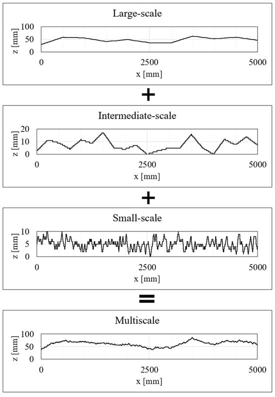
Figure 4.
Principle of multiscale trace development by superimposing daughter traces of different roughness generated by a random field model. At 1 mm increments on the x-axis, the large-, intermediate-, and small-scale traces (or height values on the z-axis) were superimposed to create the multiscale trace at the base of the figure.
The z values of each trace were integer values between 0 and 100. The random field model generated values with decimal places; however, each height value (z) was rounded to the nearest whole number to prescribe a pixel coordinate within the output images (i.e., pixels form an array with positions 0, 1, 2, …, 3, etc.). The resulting roughness characteristics of each trace are summarised in Table 1 and they are shown in Figure 5.
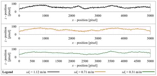
Figure 5.
Plots of the three generated multi-scale traces used during the investigations into the digitisation methodology. Please note the z-axis is not proportionally scaled to the x-axis and exaggerates the profile of the traces vertically. The axes are displayed in pixels rather than millimetres because these data were directly translated to image format to commence the next steps. The legend identifying each trace is located at the base of the figure, and further, the traces are ordered roughest to smoothest from top to bottom.
The control traces were then plotted onto an image (format png); with the trace plotted black, and the remainer of the image plotted white. The images were 5000 pixels wide and 200 pixels tall. The thickness of the trace on the image was arbitrarily set to 7 pixels to increase visibility of the trace on the photographs to be taken. Such a thickness is consistent with photographs of real discontinuity traces. At a given x-coordinate, the z-coordinate of the trace was in the middle pixel of the seven within the thickness of the trace.
Each seed trace image was then densified in Photoshop using the bilinear interpolation method. The final image was 30,000 pixels wide and 1200 pixels tall. The purpose of densifying each image at this stage was to allow for high-resolution input of data into Blender to best simulate a real discontinuity [57]. This was performed now rather than during the generation step due to limitations in the RFM; data had to be generated at 1 mm increments (or single-pixel increments) to maintain control of the input statistics. Please note the bilinear interpolation method was deemed most suitable by trial and error.
A summary of inputs to the random field model can be found in Appendix A.
2.2. Trace Photography and Digitisation
The seed trace digitisation methodology was applied to the generated seed trace data in a variety of cameras distance and orientations, relative the rock face, to quantify the associated errors on roughness characterisation. The control traces printed onto high resolution images were input into Blender, for photographs to be virtually captured, replicating real scenarios in a virtual environment. Blender (v4.0) is an opensource 3D creation software that supports 3D models, lighting, camera positioning and setup, simulations, and rendering, amongst other features [59]. Blender has been used in the scientific community for the presentation of data, medical scans, and animations [60,61]. A key capability of Blender is being able to capture images of 3D scenes with cameras of different technical specifications and orientations and in various lighting conditions. The images captured within Blender closely represent those that would be captured in the same scenarios in the ‘real world’. The virtual camera properties used for the investigations presented in this paper within Blender are summarised in Table 2.
Table 2.
Properties of the virtual camera used in Blender.
For all Blender scenarios considered, a vertical rock face was used, and sunlight was applied to the trace at 45° to simulate ideal lighting conditions (i.e., uniform, and consistent daylight on the rock face). Lens distortion was minimised by adopting a prime lens (i.e., fixed focal length) for all images captured in Blender. The boundary of the output images was checked for square within Photoshop, no obvious curved distortions were noticed at each camera position, so no corrections for lens distortion were required.
A specific programme of investigations was developed to study the effect of several relevant parameters, one at a time, on the possible error made on the roughness quantification.
Part 1: The error due to developing the input seed trace using the random field model was evaluated by applying those data into png image format and densifying the input image for use in Blender. Errors may arise from possible image compression during the formation of the png image or during densification. For this study, Blender was not used. The three control traces were developed and then put straight into the Python trace extraction script, bypassing any photography to determine the magnitude of any systematic errors.
Part 2: The effect of ground sampling distance (GSD) was investigated. GSD is a parameter commonly used in scientific photography and photogrammetry. It describes the real length in the scene which a pixel covers in mm per pixel. The influence of GSD on roughness data was investigated to determine the optimal distance to position a camera. For this part, the camera is ideally orientated perpendicular in all directions to the rock face the trace is exposed on.
Part 3: The error arising from camera rotation around the z-axis was investigated (see Figure 6 for axis definition). The idea is to simulate human error in positioning the camera perpendicular from the rock face the trace is exposed on with the camera oriented toward the centre. Each camera position relative to the seed trace is shown in Figure 7. Angles of 90°, 85°, 80°, and 75° were considered.
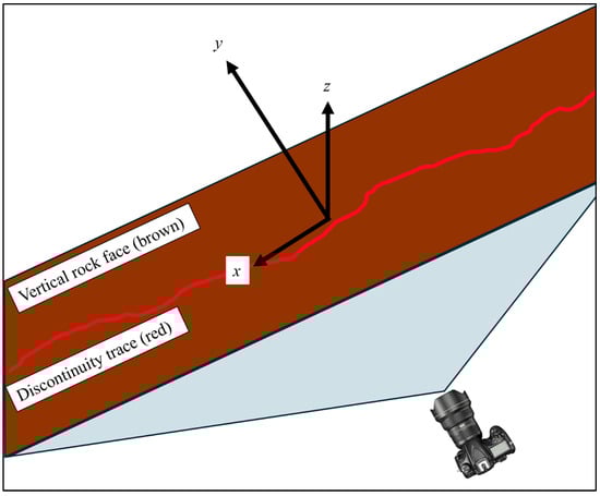
Figure 6.
Top view of an inclined rock face (in brown) containing a discontinuity (red) and showing the local x, y, and z axes. The z-axis is always vertical, the x-axis is horizontal and parallel with the rock face, and the y-axis is horizontal and perpendicular to the rock face.
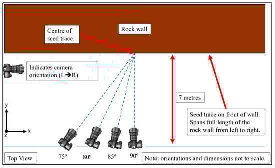
Figure 7.
A top view visual representation of the four camera positions investigated to determine the error induced in output seed trace data due to orientation around the z-axis. The cameras are aimed towards the centre of the seed trace and are oriented parallel with ground level.
Part 4: The effect of camera rotation around the x-axis was investigated (see Figure 6 for axis definition). Here, two angles are relevant, as illustrated in see Figure 8c: the angle between the rock face and the camera orientation (denoted by ) and the angle between the rock face and the average discontinuity plan (denoted by ). The latter angle’s relevance lies in the fact that the asperity heights should be measured perpendicular to the average discontinuity plane. In any other position than a discontinuity plane perpendicular to the rock face, the asperity heights are seen larger than they are (i.e., exaggerated by perspective), and a geometric correction should be applied. The correction is expressed in Equation (1):
where z is the corrected height value representative of the trace amplitude perpendicular to the discontinuity plane, is the distorted amplitude of the seed trace captured in the original image of the seed trace (see Figure 8a), is the angle between to average plane of the rock face where the seed trace is exposed upon and the orientation vector of the camera (see Figure 8c), and is the angle between the average discontinuity plane and the average plane of the rock face where the seed trace is exposed upon (see Figure 8c). It should be noted that the camera is positioned perpendicular to the rock face around the z-axis (see Figure 8b) and level. Unfortunately, it is not possible to change angle using Blender, so a constant value of 90° was adopted. Angle was varied from 90° to 45° in 5° increments. The data were then corrected at each data point during post-processing using Equation (1). An example of a planar rock face containing a trace oriented 15° from perpendicular is shown in Figure 9.
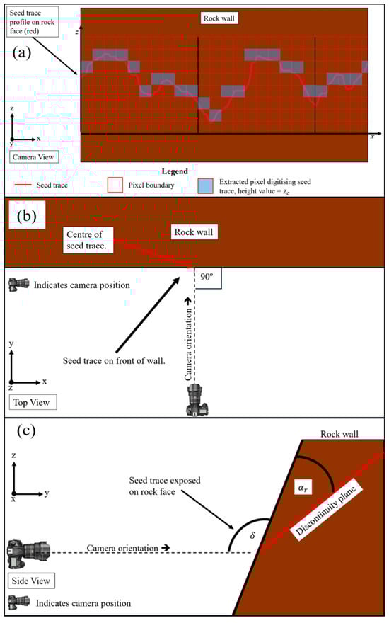
Figure 8.
(a) Camera view of the discontinuity on the rock face. The red boxes indicate a hypothetical array of pixels that would form the image structure on capture. The blue shaded pixels indicate the profile of the trace that could be extracted using the digitisation methodology at this hypothetical resolution. (b) Top view. The camera is oriented perpendicular to the rock face around the z-axis. (c) Side view shows the rock face oriented non-perpendicularly to ground level, and the discontinuity plane non-perpendicularly to the rock face. The two angle parameters used to correct for rotation around the x-axis are also indicated.
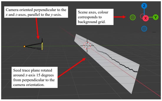
Figure 9.
Example of a Blender scene constructed to simulate an angle oblique to perpendicular between the camera direction and the seed trace plane around the x-axis. The camera position is represented by the orange dot/circle to the left of the image and the black and white trace image plane to the right.
Part 5 combines incremental rotations around x and z axes to assess the possible compounding digitising errors due to rotation around two axes. This was conducted to simulate the potential for poor put results when the operator capturing the images is not careful or diligent. Like part 3 above, the camera was positioned with rotation around the z-axis at 5° from perpendicular; however, the trace was also tilted by 5° at the same time rather than staying perpendicular. The trace and camera were oriented at the same respective orientations from 90° to 75° at 5° increments.
A summary of inputs for each part of the investigation can be found in Table 3. The output images captured in Blender were all densified during post-processing prior to extracting the coordinates of the trace using the nearest neighbour approach in Photoshop [57]. The orientation of each is always the same for each of the investigations referred to above. The z-axis is always vertical, the x-axis is parallel to the rock face plane and is level, the y-axis is perpendicular to the rock face plane and level, and the origin of axes is set at the centre of the seed trace. This is visually demonstrated in Figure 6.
Table 3.
Summary of all parameters used during the investigations into the trace digitisation approach. Contained within parts 2, 3, and 5 are subsections (labelled a, b, c, …, etc.) which explain the variations tested. In part 2, for example, the 5 m trace with input image size of 30,000 × 12,000 pixels was captured at 12 m, 9 m, and 7 m to result in GSDs of 2.2, 1.6, and 1.3 mm/pixel.
2.3. Calculation of Errors
The investigations into the digitisation approach were evaluated by calculating the relative error on sdi and the standard deviation of absolute errors for each output trace in each different scenario. The relative error on sdi (%) was calculated by Equation (2) and the standard deviation of absolute errors was calculated by Equation (3).
where is the relative error percentage of sdi, is the sdi of the output trace of a particular scenario, and is the sdi of the original input trace data.
where is the standard deviation of absolute errors, is each height value of the output trace at x position i, is each height value of the original trace at x position i, is the average of height differences between the output and original traces at 1 mm increments on the x-axis, and N is the number of points on the trace. In most cases, N was equal to 5001; however, some investigations used smaller traces, in which case N was equal to 1001.
Quantification of the standard deviation of absolute errors was conducted to provide readers (and the authors) with additional insight into how the digitisation method behaved. Just because the quantification of sdi may be accurate in the tested scenarios does not necessarily indicate the method is accurate when the absolute errors are high.
Like quantifying the errors on trace digitisation, errors on the predictions of peak and residual shear strength were also calculated relative to the real values using Equation (4) and Equation (5), respectively.
where and are the relative error of the peak and residual shear strength predictions, and and the peak and residual shear strength predictions made with known error input of sdi, and and are the peak and residual shear strength predictions made with no error input of sdi.
2.4. Influence of Digitisation Error on Shear Strength Predictions
The digitisation of a seed trace yields the roughness data required to make predictions of peak and residual shear strength using the Newcastle discontinuity shear strength model (NDSS) and the continued fraction regression (CFR) model [51]. To assess the significance of the error made during data capturing on shear strength prediction, a parametric study was conducted using the CFR model, which is more computationally efficient than the NDSS.
The CFR model was developed by applying a continued fraction mathematical regression model to a set of 14,000 shear strength predictions produced by the Newcastle discontinuity shear strength model. The primary inputs to the model are the sdi (in m/m) computed in the shear direction, the material strength parameters of the rock (, mi, and ), and effective normal stress (). The model predicts the number of sheared facets (NCFo) of a 3D surface with a 4 m2 projected area (Atot-o) at a 1 mm spatial increment (Reso). The model is defined mostly by Equation (6) (further broken down into Equations (7)–(9)):
where
The sdi may be computed from a 3D point cloud of a surface or from a trace exposed on a rock face and should ideally be computed in the shear direction whenever possible to avoid effects of possible anisotropy.
Here, the sdi was taken from the three generated seed traces used throughout the paper equal to 1.12 m/m, 0.71 m/m, and 0.31 m/m, respectively. Based on the prediction of NCFo, the CFR model may predict peak and residual shear strength using Equation (10) and Equation (11), respectively.
The Hoek brown criterion is used to derive both and for a given stress state [62] by Equations (12) and (13).
where is the local normal stress acting on contributing asperities, mi and are the material parameter and intact unconfined compressive strength of the Hoek Brown criterion obtained by fitting experimental triaxial data, and is defined as
where and .
The material strength inputs for the parametric study are presented in Table 4.
Table 4.
Parameters used as input to the CFR model for the investigation into peak shear strength prediction error induced by error on sdi. The strength parameters correspond to limestone previously tested [43].
The three input traces with standard deviation of gradients (sdi) of 0.31 m/m, 0.71 m/m, and 1.12 m/m were also used as a base for the inputs. The sdi was input with relative error ranging from −20% to +20% at 5% increments at a variety of normal stresses. The normal stress scenarios were 0.01 MPa, 0.1 MPa, 1 MPa, 10 MPa, and 100 MPa. This process was conducted for each seed trace resulting in plots of input sdi error and output relative errors of peak and residual shear strength.
3. Results
3.1. Error Due to Data Extraction Algorithm and Image Densification
This section reports the results of the investigation into systematic error produced by generating png-format images of the control traces that underwent pixel densification by the bilinear interpolation method in Photoshop. Each trace image was processed using a trace coordinate extraction script written in Python. Here, Blender was not used, and photographs of the traces were not taken. Rather, the objective was to assess the error resulting from the image creation, densification, and data extraction. The error relative to the original trace data both for sdi and absolute error is shown in Figure 10a and Figure 10b, respectively. See Section 2.3 for definitions and the calculations of errors.
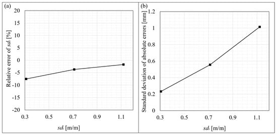
Figure 10.
(a) Values of relative error of standard deviation of gradients (sdi) for each of the three control traces identifiable by their standard deviation of gradients. (b) Values of standard deviation of absolute error (of heights) for each of the three control traces. The amplitude of all three traces is approximately 50–60 mm, making the standard deviation of absolute errors between 0.2 mm and 1 mm relatively negligible.
The results show that the process of converting the generated seed trace data to a png image, its densification, and then the extraction of the trace using a python script does result in some error. Interestingly, the rougher the surface, the higher the absolute error on heights (Figure 10b) but the lower the relative error (absolute) on gradients (Figure 10a). The fact that the relative error on gradients is lower for rougher traces can be attributed to simple math; a higher sdi on the denominator of the relative error calculation results in a smaller relative error percentage. The increasing relationship between the standard deviation of absolute error and roughness can be attributed to the formation of the png image type, where hard edges are slightly softened during development using deflate compression [63]. The relative error on sdi is negative for all three traces, implying that the process slightly underestimates sdi. This underestimation can again be attributed to the formation of the image type, where some extremity asperity peaks are softened, resulting in a slightly smoother trace profile.
The standard deviations of absolute error for each trace are maximum ~1 mm for all traces. Overall, the error due to the image processing and extraction Python script falls within the range −7.5% to −2%, which is quite low.
3.2. Error Due to Ground Sampling Distance (GSD)
In this section, the image of each control trace was imported to Blender, photographs were taken with the virtual camera (orientated ideally, i.e., perpendicularly, to the rock face), the photographs were densified, and the roughness profile was extracted. The distance between the rock face and the camera was increased from 6 m to 12 m. This range of distances results in a GSD ranging from 1.1 mm/pixel to 2.2 mm/pixel given the resolution of the camera (refer to Table 2). This process was applied to the three control traces of Section 2.1; however, eventually the entire trace was not contained within the image frame as the camera was positioned closer. To continue investigating at GSDs less than 1.2 mm/pixel, each trace was cropped to the first 1 m of length, enabling the entire trace to be contained within the image frame. The relative errors for these cases were calculated relative to the trace statistics representative of the trace length captured within the image frame over 1 m of length and the results depict this in Figure 11.
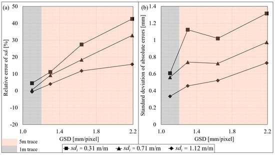
Figure 11.
(a) The relative error of standard deviation of gradients (in m/m) for different ground sampling distances. The results for each trace, varying in roughness, are identifiable using the legend at the base of the figure. (b) Results showing the standard deviation of absolute errors at each ground sampling distance. The results for each trace, varying in roughness, are identifiable using the legend at the base of the figure.
Figure 11 shows the evolution of relative error on sdi and standard deviation of absolute error on heights as the GSD increases from 1.1 mm/pixel to 2.2 mm/pixel. When the camera was positioned too close to the rock face (in our case, closer than 7 m), it was not possible to capture the full 5 m of trace length. In that case, only 1 m of trace was photographed, analysed, and compared to the same 1 m of control trace.
The overall trend was that increasing the GSD resulted in increased error, both relative and absolute. The GSD correlates to the resolution of the photograph: the higher the GSD, the more physical area a pixel covers, and hence, the lower the resolution. Roughness information was lost as GSD increased, which explains the increased error. These results indicate that a GSD equal to 1 mm/pixel delivered the best results overall, because the relative error on standard deviation of gradients trended towards zero for all traces. Whilst the results presented in Figure 11 indicate that output data generally improve as the camera gets closer to the seed trace, the access to and size of the trace may limit the ability to place the camera very close to the rock face. Indeed, in this study, the trace was required to be captured in a single photograph. A GSD of 1.36 mm/pixel was practical as it corresponded to 7.5 m from the rock face for this camera and it allowed for the capture of the entire 5 m trace.
3.3. Errors Due to Camera Rotation Around the z-Axis
In this section, the images of the three control traces were imported into Blender and photographs were taken with the camera positioned at various positions to the rock face such that the camera was not perpendicular to the trace plane around the z-axis. The errors were computed for each camera orientation to reveal the effect of camera rotation around the z-axis (refer to Figure 7). The relative error on sdi is shown in Figure 12a, and the standard deviation of absolute errors is shown in Figure 12b.
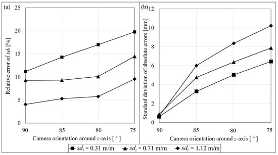
Figure 12.
(a) Results showing the relative error of the output standard deviation of gradients from the original seed trace data at each camera rotation around the z-axis. The results for each trace, varying in roughness, are identifiable using the legend at the base of the figure. (b) Results showing the standard deviation of absolute errors at each camera rotation around the z-axis. The results for each trace, varying in roughness, are identifiable using the legend at the base of the figure.
As seen in Figure 12 any deviation around the z-axis from perpendicular results in a decay in data quality from both a gradient perspective and an absolute error perspective. The range of absolute errors increases (represented by an increase in standard deviation) as the camera is rotated further from perpendicular for each trace. The roughest trace (sdi = 1.12 m/m) experienced the greatest increase in absolute error as the camera increased its rotation from perpendicular to the trace. As the camera rotated around the z-axis, roughness data were lost, with all traces exhibiting a standard deviation of absolute error greater than 3 mm after only 5° rotation. The data loss exhibited by the output traces occurred due to parts of the rough profile falling within the resolution of the image, disabling the ability to characterise the profile by pixel location.
These results highlight the importance of ensuring a perpendicular orientation of the camera relative to the rock face. This can be achieved with relatively high accuracy using basic measuring techniques and survey data on site.
3.4. Errors Due to Camera Rotation Around the x-Axis
In this section, the three input traces were imported into Blender and incrementally rotated around the x-axis at 5° increments to determine the error where the camera cannot capture images of the trace whilst perpendicular to the trace plane around the x-axis. The errors were computed for each trace orientation to reveal the effect of a camera rotation around the x-axis (refer to Figure 9). Prior to evaluating the error on the output traces, each output was geometrically corrected using Equation (1). The relative error on sdi is shown in Figure 13a and the standard deviation of absolute errors is shown in Figure 13b.
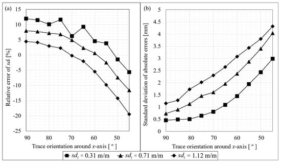
Figure 13.
(a) The relative error of standard deviation of gradients (in m/m) for different rotations of the seed trace or camera around the x-axis. The results for each trace, varying in roughness, are identifiable using the legend at the base of the figure. (b) Results showing the standard deviation of absolute errors at each camera rotation around the x-axis. The results for each trace, varying in roughness, are identifiable using the legend at the base of the figure.
The results presented in Figure 13 show that, as the camera progressively rotates from its initial position (angle of 90°), the initially positive relative error reduces to 0% for an angle that depends on the roughness of the trace, and then its magnitude increases again, this time in the negative range. For the roughest trace, it takes a rotation of 40° to reach a relative error of 15% in magnitude. In contrast, for the smoothest trace, the maximum magnitude of relative error measured in 12%. Figure 13b shows a consistent increase in absolute error on heights as the camera orientation increases. The rougher the trace (or surface), the higher the absolute error.
Considering these results, one would suggest that rotations over 35° from vertical give poor results that may not be reliable for accurate shear strength prediction. However, Figure 13b indicates that the data suffered a notable decay in quality from inclinations over 15° from vertical, demonstrated by the standard deviation of absolute errors exceeding 2 mm for the smoothest trace in Figure 13b. Hence, whilst the relative errors on sdi remain within ±10% for rotations up to 35° from perpendicular, the actual output traces are not necessarily representative of the real trace because the absolute errors increase with any rotation.
Data quality decayed as the seed trace plane was rotated around the x-axis because some asperities’ amplitude fell within the resolution of the image. Hence, some asperities were lost due to the camera’s inability to prescribe them a location within a single pixel. This is demonstrated in Figure 14b after Figure 14a is rotated by 15° around the horizontal axis. The shaded pixel boxes show the locations of pixels extracted to digitise the seed trace. The shaded pixel profile for the image captured perpendicular to the seed trace (Figure 14a) is clearly rougher and captures more roughness data than the image captured at 15° to the seed trace (Figure 14b).
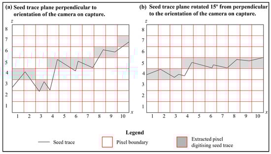
Figure 14.
Roughness data begin to fall into plane, reducing asperity amplitude when the trace is rotated around the x-axis from 90° (shown in part a on the left of the figure) by 15° (shown in part b on the right of the figure). Eventually, some roughness data fall within the resolution of the image, causing data loss.
Based on the results of this investigation presented in Figure 13 and Figure 14, it is recommended that the angle between the camera and the seed trace plane does not exceed 15° from perpendicular.
As mentioned in Section 2.2, it was not possible to change angle using Blender, so a constant value of 90° was adopted, and only angle was varied (refer to Figure 8). Whilst was not independently varied, the simulations presented above cover its effects on results because the geometric influence of is the same as . This investigation resulted in a recommendation for not to exceed 15° from perpendicular; this can be extrapolated to a basic geometric relations ship with . Geometrically, no distortion of the trace will occur when the sum of and is 180° (i.e., the camera direction is parallel to the discontinuity plane). Hence, the sum of and should not be less than 165° in accordance with the findings in this section; this allows for a combination of these angles where required.
3.5. Effect of Combined Rotations
In this section, the three input traces were imported into Blender and images were captured whilst incrementally moving the camera to rotate its perspective around the z-axis and tilting the trace around the x-axis simultaneously at 5° increments. The purpose of the investigation was to determine whether the output trace errors were exaggerated by a combination on rotations when an operator capturing the images is not careful or diligent on site.
The errors were computed for each trace orientation to reveal the effect of combined rotations (refer to Figure 7 and Figure 9). Prior to evaluating the error on the output traces, each output was geometrically corrected using Equation (1) to correct for the x-axis rotation. The relative error on sdi is shown in Figure 15a, and the standard deviation of absolute errors is shown in Figure 15b.
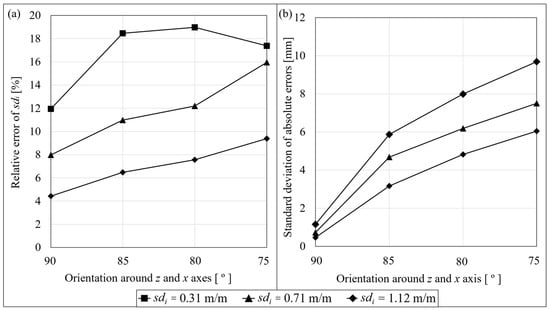
Figure 15.
(a) Results showing the relative error of the output standard deviation of gradients from the original seed trace data at each orientation around the z and x axes. (b) Results showing the standard deviation of absolute errors at each orientation around the z and x axes.
The output traces for the combined rotations exhibited features of the results shown in Figure 12 and Figure 13 where the rotations were individually investigated. The relative error on sdi exhibited nearly the same profile and magnitude for all traces as the errors for rotation around the z-axis (i.e., Figure 12a). The smoothest trace (sdi = 0.31 m/m) error began to reduce from 80° to 75°; possibly, this was the influence of rotation around the x-axis where the relative error decreases from positive to negative with rotation (refer to Figure 13a). The standard deviation on absolute errors exhibited little difference to the errors where only the z-axis was rotated (refer to Figure 12b).
Based on these observations, a combination of rotations does not necessarily exaggerate the errors on output traces using the digitisation methodology. However, the results reinforce the importance of aligning the camera perpendicular to the rock face ideally in all directions. If the camera cannot be orientated perpendicular around the x-axis, a geometric correction may be made. Unfortunately, no real solution allows for rotation around the z-axis due to complex perspective distortions. Hence, alignment around the z-axis remains critical to check to ensure quality trace output results.
3.6. Effect of Roughness Error on Shear Strength Predictions
Figure 16 presents the relative error on peak and residual shear strength prediction resulting from a relative error input on the standard deviation of gradients sdi, as per Section 2.4. All other input parameters for the CFR model are given in Section 2.4. Each sub-figure corresponds to a trace with a given sdi, on which the error is made. The results are plotted for a variety of normal stresses denoted in the legend at the base of the figure.
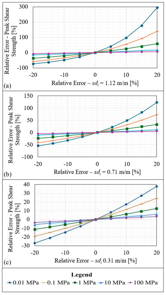
Figure 16.
Peak shear strength relative errors induced by various input errors of sdi. The three input traces are plotted separately in parts a to c, and various normal stresses are shown in each plot denoted by the different symbols and coloured lines. (a) The peak shear strength prediction errors relative to the correct input of sdi for the input of sdi = 1.12 m/m. (b) The peak shear strength prediction errors relative to the correct input of sdi for the input of sdi = 0.71 m/m. (c) The peak shear strength prediction errors relative to the correct input of sdi for the input of sdi = 0.31 m/m.
The relative errors on strength and on standard deviation are positively correlated: an overestimation of roughness yields an overestimation of strength, which is consistent with results from the literature. The most important observation is the disproportionate influence of input error of sdi on predictions of peak shear strength. This strong effect is exacerbated under low normal stress and high roughness: for a stress of 0.01 MPa and a rough trace (sdi = 1.12 m/m), an error of +20% on sdi yields in a peak shear strength prediction error of +300%. However, results improved with increases in normal stress, with predictions of peak shear strength falling within ±10% relative error at 100 MPa normal stress. As seen in Figure 16b,c, the sensitivity to error input of sdi reduces with roughness, with the maximum errors decreasing to 125% and 38%, respectively. These findings highlight the need to take extra care when assessing the roughness of rougher discontinuities subjected to low normal stress.
Residual shear strength is dependent on the number of contributing facets as defined by Equation (11). Despite this, the influence of sdi error on predictions of residual shear strength is far less significant than on predictions of peak shear strength as demonstrated in Figure 17. Similarly, here, results are plotted for a variety of normal stresses denoted in the legend at the base of the figure.
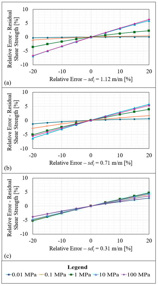
Figure 17.
Residual shear strength relative errors induced by various input errors of sdi. The three input traces are plotted separately in parts a to c, and various normal stresses are shown in each plot denoted by the different symbols and coloured lines. (a) The residual shear strength prediction errors relative to the correct input of sdi for the input of sdi = 1.12 m/m. (b) The residual shear strength prediction errors relative to the correct input of sdi for the input of sdi = 0.71 m/m. (c) The residual shear strength prediction errors relative to the correct input of sdi for the input of sdi = 0.31 m/m.
The results shown in Figure 16 and Figure 17 demonstrate the sensitivity of shear strength predictions to different input errors of sdi. These results are exacerbated by roughness and normal stress to varying degrees for both peak and residual shear strength. Unlike peak shear strength, the relative errors on predictions of residual shear strength are contained between ±7%. Predictions of residual shear strength are fundamentally less sensitive to roughness compared to peak shear strength due to their mathematical formulation [51]. The equations used to calculate peak and residual shear strength may assist the reader understand this phenomenon; refer to Equation (10) and Equation (11), respectively.
4. Discussion
4.1. Remarks on the Digitisation Methodology
The new seed trace digitisation methodology was shown to be effective in several scenarios expected to encounter in the field. The influence of camera rotation and GSD relative to the seed trace plane were investigated. The key observations taken from each investigation include the following:
The systematic relative error on sdi induced by generating images of seed trace data ranged from −1.7% to −7.5%.
The ideal conditions simulating a camera perpendicular to the seed trace plane produced a relative error on sdi from 4.1% to 11.2%, with the smoothest trace experiencing the highest relative error. For all traces, this process exhibited a maximum standard deviation of absolute errors of approximately 0.6 mm.
Rotation of the camera up to 5° from perpendicular around the z-axis resulted in suitably low relative error on sdi. Based on the results of this investigation, the camera should ideally be placed perpendicular to the rock face around the z-axis in all scenarios. Failure to do so may results in unreliable results.
Rotation of the camera around the x-axis relative to the seed trace plane was shown to be correctable for rotations up to 15° from perpendicular. Any rotations exceeding that limit began to exhibit high levels of error, especially for rough traces.
A captured ground sampling distance (GSD) equal to or better (i.e., smaller) than 1.4 mm/pixel was found best to characterise seed trace roughness. All traces exhibited greater than 10% relative error for sdi where the GSD exceeded 1.4 mm/pixel.
A combination of rotation around the z and x axes resulted in similar results to only rotating the camera around the z-axis. The combination of rotations did not exaggerate error, and this investigation reinforced the importance of orienting the camera perpendicular around the z-axis.
4.2. Ramifications of Errors on Predictions of Peak Shear Strength
The investigation into shear strength prediction errors due to input error of sdi enabled several key observations to be made:
Seed trace errors resulting in an overestimation or underestimation of sdi disproportionately influence predictions of peak shear strength but have relatively little influence on predictions of residual shear strength. This can be explained by the mathematical formulation of the CFR model, a model that is based on theoretical shear mechanics and experimentally validated.
Rougher seed traces experience greater errors in predictions of shear strength due to input errors of the standard deviation of gradients calculated at 1 mm increments (sdi).
Predictions of peak shear strength are most disproportionately influenced by input errors of sdi at normal stresses less than 1 MPa.
Peak shear strength predictions must be correctly interpreted based on the level of roughness and magnitude of normal stress to ensure predictions are made within acceptable bounds.
These observations give valuable insights into how site investigations must be conducted in the future and how predictions of shear strength made after digitising an in situ seed trace must be interpreted. Following this reasoning, the following recommendations can be made:
During a site investigation, firstly, an accurate estimation of normal stress must be gained. For discontinuities experiencing low normal stress (i.e., <1 MPa), there is less flexibility in data capture methods, limiting the following steps of the investigation. Where normal stress is low, ideal conditions (i.e., ground sampling distance (GSD) 1.4 mm/pixel, camera perpendicular to seed trace, seed trace perpendicular to rock face) must be adhered to as closely as possible to make accurate predictions of peak shear strength.
Regardless of normal stress, the seed trace digitisation methodology may be an iterative approach to ensure the process remains economical where an initial application is used to determine the approximate magnitude of sdi. Where sdi is approximately greater than 0.3 m/m, perhaps an additional application of the method is necessary where extra expense and effort is spent to improve the camera quality, camera position, or the capture GSD. This is due to rough traces producing the highest shear strength prediction errors due to input error of sdi.
The predictions of peak shear strength must be correctly interpreted based on the quality of the investigation, the magnitude of normal stress, and the magnitude of sdi in conjunction with the results shown in Figure 16. Predictions of peak shear strength for smoother discontinuities (sdi < 0.3 m/m) experiencing higher normal stress (>1 MPa) can be treated with greater confidence, especially where the trace was digitised under ideal conditions (i.e., GSD 1.4 mm/pixel, camera perpendicular to rock face, and discontinuity perpendicular to rock face).
4.3. Comments on Practical Application
The work presented in this paper gave valuable insight into further developing and applying the digitisation methodology for shear strength predictions. Based on the discussion in Section 4.1 and Section 4.2, some key tips on applying the methodology have been compiled and are summarised in Table 5.
Table 5.
A summary of practical tips on applying the digitisation methodology in the field.
4.4. Recommendations for Further Research
The work presented in this paper provides a robust foundation for digitising the seed trace data of planar seed traces in the field. However, limitations to the approach must be addressed, with further research focusing on the following issues:
Developing an approach to robustly extract the profile of a seed trace from images of real, natural rock discontinuities. The research presented in this paper focusing on simplified conditions (i.e., black and white images); however, images of natural discontinuities contain different colours which complicates the identification of the profile of the seed trace.
Lighting conditions must be considered in the future. Standard photography practices are well known and can be employed to improve the image quality (i.e., non-direct sunlight, consistent lighting across rock face). However, the influence of exposure settings and contrast is not yet understood.
Discontinuities may contain infilling, have openings, are weathered, or be mismatched. These issues are known to influence predictions of shear strength [23,24,26,35]. Additional work must be undertaken to determine how to robustly digitise a seed trace in these circumstances and also how to incorporate these properties into StADSS.
The question of how to extend the approach to discontinuities longer than 5 m needs to be addressed. A single image may not provide a suitable GSD; hence, multiple images may be required to digitise the length of a seed trace accurately. Possible avenues include panorama images and stitching trace segments after processing.
The influence of curved rock faces on seed trace data collection. Rock faces are not always planar as considered within this paper. Additional research is required to determine how much curve or undulation is acceptable before seed trace data becomes unusable with the standard approach.
5. Conclusions
A new method to digitise the in situ traces of natural rock discontinuities at full scale using high resolution images was investigated from an error’s perspective. The purpose of the research was to determine how sensitive the method is to scenarios likely to encounter in the field and how the resulting errors on trace digitisation influence predictions of shear strength made using the stochastic approach for discontinuity shear strength (StADSS) and the continued fraction regression (CFR).
Investigations into rotations of the camera and trace plane around the z and x axes, respectively, confirmed that orienting the camera perpendicular to the trace plane produces the most accurate results. Rotations around the x-axis were found to be correctable to within 15° of perpendicular, and output traces from rotations around the z-axis were only suitably accurate within 5° of perpendicular. The output traces were found to be highly sensitive to the capture ground sampling distance (GSD), and a recommendation of a GSD equal to or better than 1.4 mm/pixel was made. Combinations or rotations around the z and x axes at the same time were found not to exaggerate the output trace errors more than when the rotations occurred independently.
Lastly, predictions of peak shear strength were found to be highly sensitive to overestimations of the standard deviation of gradients calculated at 1 mm increments (sdi), especially at low normal stress. Generally, the digitisation method always slightly overestimated the sdi of the trace, which highlighted the importance of interpreting predictions of peak shear strength based on the magnitude of sdi and normal stress. Residual shear strength predictions were found to be far less sensitive to input errors of sdi. Based on the recommendations made within this paper to achieve acceptable results, predictions of peak and residual shear strength made using trace data from the digitisation methodology can be treated with confidence.
Author Contributions
All authors contributed to the study conception and design. Material preparation, data collection and analysis were performed by C.B. and O.B. The first draft of the manuscript was written by Clarence Butcher. All authors engaged in planning for the field investigation, scientific discussion during the interpretation of results, and commented on previous versions of the manuscript. All authors have read and agreed to the published version of the manuscript.
Funding
This research was funded by Australian Research Council grant number DP190101558.
Data Availability Statement
The raw data supporting the conclusions of this article will be made available by the authors on request in the spirit of collaborative research.
Acknowledgments
The authors acknowledge the financial support provided by PSM.
Conflicts of Interest
Author Robert Bertuzzi was employed by the company PSM. The remaining authors declare that the research was conducted in the absence of any commercial or financial relationships that could be construed as a potential conflict of interest.
Nomenclature
| Symbol | Units | Description |
| GSD | mm/pixel | Ground sampling distance |
| degrees | Angle between the discontinuity average plane and rock face average plane | |
| degrees | Angle between the rock face and camera orientation | |
| MPa | Hoek–Brown intact compressive rock strength | |
| - | Hoek–Brown intact material constant | |
| degrees | Basic friction angle | |
| SI | mm | Segment interval |
| mm | Correlation length | |
| mm | Trace height value at a position on the x-axis | |
| mm | Distorted trace height value captured by a camera | |
| mm | Mean of heights | |
| mm2 | Variance of heights | |
| mm | Standard deviation of heights | |
| m/m | Mean of gradients at 1 mm increment | |
| sdi | m/m | Standard deviation of gradients at 1 mm increments |
| % | Relative error percentage of sdi | |
| m/m | sdi of the output trace | |
| m/m | sdi of the original trace | |
| mm | Standard deviation of absolute errors | |
| mm | Height value of the output trace at x position i | |
| mm | Height value of the original trace at x position i | |
| mm | Average of height differences between the output and original traces | |
| N | - | Number of z coordinates in the trace |
| % | Relative error of the peak shear strength prediction | |
| MPa | Peak shear strength prediction made with known error input of sdi | |
| MPa | Peak shear strength prediction made with correct input of sdi | |
| % | Relative error of the residual shear strength prediction | |
| MPa | Residual shear strength prediction made with known error input of sdi | |
| MPa | Residual shear strength prediction made with correct input of sdi | |
| mm2 | Projected area of a triangular facet | |
| - | Number of contributing facers of the reference surface | |
| - | Number of contributing facets | |
| mm2 | Total projected area of a discontinuity | |
| mm2 | Total projected area of the reference surface | |
| c | MPa | Cohesion |
| ° | Friction angle | |
| MPa | Stress acting on an active facet | |
| Res | mm | Resolution of surface roughness data |
| Reso | mm | Resolution of the reference surface |
| N | Total force acting on the whole discontinuity | |
| MPa | Normal stress |
Appendix A
Table A1.
Summary of inputs to the 1D random field model to generate the input seed traces. See Nomenclature for definition of variables.
Table A1.
Summary of inputs to the 1D random field model to generate the input seed traces. See Nomenclature for definition of variables.
| Output sdi (Trace ID) | Large-Scale Inputs | Intermediate-Scale Inputs | Small-Scale Inputs | |||||||||
|---|---|---|---|---|---|---|---|---|---|---|---|---|
| SI | SI | SI | ||||||||||
| m/m | mm | mm | mm | mm2 | mm | mm | mm | mm2 | mm | mm | mm | mm2 |
| 1.12 | 500 | 490 | 250 | 400 | 250 | 80 | 0 | 100 | 1 | 4 | 0 | 12 |
| 0.71 | 500 | 490 | 250 | 340 | 250 | 100 | 0 | 68 | 1 | 6 | 0 | 8 |
| 0.31 | 500 | 490 | 250 | 265 | 250 | 125 | 0 | 28 | 1 | 20 | 0 | 3 |
References
- Hoek, E. Practical Rock Engineering. 2006. 341p. Available online: https://www.rocscience.com/assets/resources/learning/hoek/Practical-Rock-Engineering-Full-Text.pdf (accessed on 5 June 2024).
- Bandis, S.; Lumsden, A.C.; Barton, N.R. Experimental studies of scale effects on the shear behaviour of rock joints. Int. J. Rock Mech. Min. Sci. Geomech. Abstr. 1981, 18, 1–21. [Google Scholar] [CrossRef]
- Tatone, B.S.A.; Grasselli, G. An Investigation of Discontinuity Roughness Scale Dependency Using High-Resolution Surface Measurements. Rock Mech. Rock Eng. 2012, 46, 657–681. [Google Scholar] [CrossRef]
- Pratt, H.R.; Black, A.D.; Brace, W.F. Friction and deformation of jointed quartz diorite. In Proceedings of the 3rd ISRM Congress on Rock Mechanics, Denver, CO, USA, 1–7 September 1974; pp. 306–310. [Google Scholar]
- Barton, N.; Choubey, V. The Shear Strength of Rock Joints in Theory and Practice. Rock Mech. 1977, 10, 1–54. [Google Scholar] [CrossRef]
- Cravero, M.; Iabichino, G.; Piovano, V. Analysis of Large Joint Profiles Related to Rock Slope Instabilities. In Proceedings of the 8th ISRM Congress, Tokyo, Japan, 25–29 September 1995. [Google Scholar]
- Swan, G.; Zongqi, S. Prediction of shear behaviour of joints using profiles. Rock Mech. Rock Eng. 1985, 18, 183–212. [Google Scholar] [CrossRef]
- Fardin, N. Influence of Structural Non-Stationarity of Surface Roughness on Morphological Characterization and Mechanical Deformation of Rock Joints. Rock Mech. Rock Eng. 2008, 41, 267–297. [Google Scholar] [CrossRef]
- Fardin, N.; Feng, Q.; Stephansson, O. Application of a new in situ 3D laser scanner to study the scale effect on the rock joint surface roughness. Int. J. Rock Mech. Min. Sci. 2004, 41, 329–335. [Google Scholar] [CrossRef]
- Fardin, N.; Stephansson, O.; Jing, L. The scale dependence of rock joint surface roughness. Int. J. Rock Mech. Min. Sci. 2001, 38, 659–669. [Google Scholar] [CrossRef]
- Ueng, T.S.; Peng, I.H.; Jou, Y.-J.; Chang, Y. Scale effect on shear strength of computer-aided-manufactured-joints. J. GeoEngineering 2010, 5, 29–37. [Google Scholar]
- Hencher, S.; Toy, J.; Lumsden, A.C. Scale-Dependent Shear-Strength of Rock Joints; CRC Press: Boca Raton, FL, USA, 1993; pp. 233–240. [Google Scholar]
- Papaliangas, T.; Hencher, S.; Lumsden, A.C. Scale Independent Shear Strength of Rock Joints. Rock Mech. Rock Eng. 1994, 27, 97–107. [Google Scholar]
- Bahaaddini, M.; Hagan, P.C.; Mitra, R.; Hebblewhite, B.K. Scale effect on the shear behaviour of rock joints based on a numerical study. Eng. Geol. 2014, 181, 212–223. [Google Scholar] [CrossRef]
- Hencher, S.R.; Richards, L.R. Assessing the Shear Strength of Rock Discontinuities at Laboratory and Field Scales. Rock Mech. Rock Eng. 2015, 48, 883–905. [Google Scholar] [CrossRef]
- Patton, F.D. Multiple Modes of Shear Failure In Rock. In Proceedings of the 1st ISRM Congress, Lisbon, Portugal, 25 September–1 October 1966; p. ISRM–1CONGRESS-1966-1087. [Google Scholar]
- Tse, R.; Cruden, D.M. Estimating Joint Roughness Coefficients. Int. J. Mech. Min. Sci. Geomech. 1979, 16, 303–307. [Google Scholar] [CrossRef]
- Maerz, N.H.; Franklin, J.A.; Bennett, C.P. Joint roughness measurement using shadow profilometry. Int. J. Rock Mech. Min. Sci. Geomech. Abstr. 1990, 27, 329–343. [Google Scholar] [CrossRef]
- Ge, Y.; Kulatilake, P.H.S.W.; Tang, H.; Xiong, C. Investigation of natural rock joint roughness. Comput. Geotech. 2014, 55, 290–305. [Google Scholar] [CrossRef]
- Casagrande, D. A Stochastic Approach for the Shear Strength of Rock Discontinuities. Ph.D. Thesis, University of Newcastle, Callaghan, Australia, 2018. [Google Scholar]
- Jeffery, M. A Preliminary Large Scale Validation of the Stochastic Approach for Discontinuity Shear Strength (STADSS). Ph.D. Thesis, University of Newcastle, Callaghan, NSW, Australia, 2021. [Google Scholar]
- Ladanyi, B.; Archambault, G. Shear strength and Deformability of Filled Indented Joints. In Proceedings of the 1st International Symposium on Geotechnics of Structurally Complex Formations, Capri, Italy, 19–21 September 1977; Volume 1, pp. 317–326. [Google Scholar]
- Papaliangas, T.; Hencher, S.R.; Lumsden, A.C.; Manolopoulou, S. The effect of frictional fill thickness on the shear strength of rock discontinuities. Int. J. Rock Mech. Min. Sci. Geomech. Abstr. 1993, 30, 81–91. [Google Scholar] [CrossRef]
- Tating, F.; Hack, H.; Jetten, V.G. Weathering effects on discontinuity properties in sandstone in a tropical environment: Case study at Kota Kinabalu, Sabah Malaysia. Bull. Eng. Geol. Environ. 2014, 74, 427–441. [Google Scholar] [CrossRef]
- Indraratna, B.; Premadasa, W.N.; Brown, E.T.; Gens, A.; Heitor, A. Shear strength of rock joints influenced by compacted infill. Int. J. Rock Mech. Min. Sci. 2014, 70, 296–307. [Google Scholar] [CrossRef]
- Indraratna, B.; Oliveira, D.A.F.; Jayanathan, M. Revised Shear Strength Model for Soil-Infilled Rock Joints Considering Over-Consolidation Effect. In Proceedings of the SHIRMS 2008: First Southern Hemisphere International Rock Mechanics Symposium, Perth, Australia, 16–19 September 2008; pp. 523–532. [Google Scholar]
- Indraratna, B.; Mylvaganam, J. Measurement of pore water pressure of clay-infilled rock joints during triaxial shearing. Géotechnique 2005, 55, 759–764. [Google Scholar] [CrossRef]
- Brekke, T.L.; Howard, T.R. Stability problems caused by seams and faults. In Proceedings of the North American Rapid Excavation and Tunneling Conference, Chicago, IL, USA, 5–7 June 1972; pp. 25–41. [Google Scholar]
- Grasselli, G.; Egger, P. Constitutive law for the shear strength of rock joints based on three-dimensional surface parameters. Int. J. Rock Mech. Min. Sci. 2002, 40, 25–40. [Google Scholar] [CrossRef]
- Aydan, Ö.; Shimizu, Y.; Kawamoto, T. The anisotropy of surface morphology characteristics of rock discontinuities. Rock Mech. Rock Eng. 1996, 29, 47–59. [Google Scholar] [CrossRef]
- Kulatilake, P.H.S.W.; Shou, G.; Huang, T.H.; Morgan, R.M. New peak shear strength criteria for anisotropic rock joints. Int. J. Rock Mech. Min. Sci. Geomech. Abstr. 1995, 32, 673–697. [Google Scholar] [CrossRef]
- Shang, J.; West, L.J.; Hencher, S.R.; Zhao, Z. Geological discontinuity persistence: Implications and quantification. Eng. Geol. 2018, 241, 41–54. [Google Scholar] [CrossRef]
- Shang, J.; Hencher, S.R.; West, L.J.; Handley, K. Forensic Excavation of Rock Masses: A Technique to Investigate Discontinuity Persistence. Rock. Mech. Rock. Eng. 2017, 50, 2911–2928. [Google Scholar] [CrossRef]
- Paronuzzi, P.; Rigo, E.; Bolla, A. Back-Analysis of a Failed Rock Wedge Using 214 a 3D Numerical; Springer: Berlin/Heidelberg, Germany, 2015; pp. 1225–1229. [Google Scholar] [CrossRef]
- Ríos-Bayona, F.; Andersson, E.; Johansson, F.; Mas Ivars, D. The importance of accounting for matedness when predicting the peak shear strength of rock joints. IOP Conf. Ser. Earth Environ. Sci. 2021, 833, 012017. [Google Scholar] [CrossRef]
- Zhao, J. Joint surface matching and shear strength part A: Joint matching coefficient (JMC). Int. J. Rock Mech. Min. Sci. 1997, 34, 173–178. [Google Scholar] [CrossRef]
- Yang, Z.Y.; Lo, S.; Di, C. Reassessing the Joint Roughness Coefficient (JRC) Estimation Using Z2. Rock Mech. Rock Eng. 2001, 34, 243–251. [Google Scholar] [CrossRef]
- Jeffery, M.; Huang, J.; Fityus, S.; Giacomini, A.; Buzzi, O. A rigorous multiscale random field approach to generate large scale rough rock surfaces. Int. J. Rock Mech. Min. Sci. 2021, 142, 104716. [Google Scholar] [CrossRef]
- Buzzi, O.; Casagrande, D. A step towards the end of the scale effect conundrum when predicting the shear strength of large in situ discontinuities. Int. J. Rock Mech. Min. Sci. 2018, 105, 210–219. [Google Scholar] [CrossRef]
- Buzzi, O.; Casagrande, D.; Giacomini, A. A new approach to avoid scale effect when predicting the shear strength of large in situ discontinuity. In Proceedings of the 70th Candian Geotechnical Society Conference: 70 Years of Canadian Geomechanics and Geoscience, GeoOttawa 2017, Ottawa, ON, Canada, 1–4 October 2017; Canadian Geotechnical Society: Richmond, BC, Canada, 2017; Volume 8. [Google Scholar]
- Casagrande, D.; Buzzi, O.; Giacomini, A.; Lambert, C.; Fenton, G. A New Stochastic Approach to Predict Peak and Residual Shear Strength of Natural Rock Discontinuities. Rock Mech. Rock Eng. 2018, 51, 69–99. [Google Scholar] [CrossRef]
- Jeffery, M.; Lapastoure, L.M.; Giacomini, A.; Fityus, S.; Buzzi, O. Development of an improved semi-analytical model for desribing the shear strength of rock joint disconitnuities. In Proceedings of the 12th ANZ Young Geotechnical Professionals Conference (12YGPC) in Hobart, Hobart, Australia, 7–9 November 2018. [Google Scholar]
- Butcher, C.; Buzzi, O.; Giacomini, A.; Bertuzzi, R.; Griffiths, D.V.; Fityus, S. Shear Strength of a Large Limestone Discontinuity: In Situ Pull Test and Prediction. Rock Mech. Rock Eng. 2024. [Google Scholar] [CrossRef]
- Uotinen, L.; Torkan, M.; Baghbanan, A.; Hernández, E.C.; Rinne, M. Photogrammetric Prediction of Rock Fracture Properties and Validation with Metric Shear Tests. Geosciences 2021, 11, 293. [Google Scholar] [CrossRef]
- Jeffery, M.; Huang, J.; Fityus, S.; Giacomini, A.; Buzzi, O. A Large-Scale Application of the Stochastic Approach for Estimating the Shear Strength of Natural Rock Discontinuities. Rock Mech. Rock Eng. 2023, 56, 6061–6078. [Google Scholar] [CrossRef]
- Haneberg, W. Directional Roughness Profiles From Three-Dimensional Photogrammetric or Laser Scanner Point Clouds; Taylor & Francis: Abingdon, UK, 2007; Volume 1, pp. 101–106. [Google Scholar]
- Moosavi, M.; Rafsanjani, H.N.; Mehranpour, M.H.; Nazem, A.; Navabi, A. An Investigation of Surface Roughness Measurement in Rock Joints with a 3D Scanning Device; ISRM SINOROCK: Shanghai, China, 2013. [Google Scholar]
- Feng, Q.; Fardin, N.; Jing, L.; Stephansson, O.S. A New Method for In-situ Non-contact Roughness Measurement of Large Rock Fracture Surfaces. Rock Mech. Rock Eng. 2003, 36, 3–25. [Google Scholar] [CrossRef]
- Reid, T.R.; Harrison, J.P. A semi-automated methodology for discontinuity trace detection in digital images of rock mass exposures. Int. J. Rock Mech. Min. Sci. 2000, 37, 1073–1089. [Google Scholar] [CrossRef]
- Hadjigeorgiou, J.; Lemy, F.; Côté, P.; Maldague, X. An Evaluation of Image Analysis Algorithms for Constructing Discontinuity Trace Maps. Rock Mech. Rock Eng. 2003, 36, 163–179. [Google Scholar] [CrossRef]
- Buzzi, O.; Jeffery, M.; Moscato, P.; Grebogi, R.; Haque, M. Mathematical Modelling of Peak and Residual Shear Strength of Rough Rock Discontinuities Using Continued Fractions. Rock Mech. Rock Eng. 2024, 57, 851–865. [Google Scholar] [CrossRef]
- Bousaid, A.; Theodoridis, T.; Nefti-Meziani, S.; Davis, S. Perspective Distortion Modeling for Image Measurements. IEEE Access 2020, 8, 15322–15331. [Google Scholar] [CrossRef]
- Vangorp, P.; Richardt, C.; Cooper, E.; Chaurasia, G.; Banks, M.; Drettakis, G. Perception of Perspective Distortions in Image-Based Rendering. ACM Trans. Graph. 2013, 32, 1–12. [Google Scholar] [CrossRef]
- Lee, T.-Y.; Chang, T.-S.; Lai, S.-H. Correcting radial and perspective distortion by using face shape information. In Proceedings of the 2015 11th IEEE International Conference and Workshops on Automatic Face and Gesture Recognition (FG), Ljubljana, Slovenia, 4–8 May 2015; Volume 1, pp. 1–8. [Google Scholar]
- Valente, J.; Soatto, S. Perspective distortion modeling, learning and compensation. In Proceedings of the 2015 IEEE Conference on Computer Vision and Pattern Recognition Workshops (CVPRW), Boston, MA, USA, 7–12 June 2015; pp. 9–16. [Google Scholar]
- Aloimonos, J.Y. Perspective approximations. Image Vis. Comput. 1990, 8, 179–192. [Google Scholar] [CrossRef]
- Butcher, C.; Buzzi, O.; Bertuzzi, R.; Griffiths, D.V. Capturing the roughness of discontinuity traces in the field with high accuracy: The effect of photograph resolution. In Proceedings of the ISRM 15th International Congress on Rock Mechanics and Rock Engineering & 72nd Geomechanics Colloquium—Challenges in Rock Mechanics and Rock Engineering, Salzburg, Austria, 9–14 October 2023; pp. 2862–2867. [Google Scholar]
- Müller, S.; Schüler, L.; Zech, A.; Hesse, F. GSTools v1.3: A Toolbox for Geostatistical Modelling in Python. Geosci. Model Dev. 2021, 15, 3161–3182. [Google Scholar] [CrossRef]
- Blender. About Page. 2024. Available online: https://www.blender.org/about/ (accessed on 6 February 2024).
- Kent, B.R. 3D Scientific Visualisation with Blender; Springer: Berlin/Heidelberg, Germany, 2019. [Google Scholar]
- Mastrofini, A. Scientific Animation with Blender. 2023. Available online: https://alessandromastrofini.it/2023/12/18/scientific-animation-with-blender/ (accessed on 6 February 2024).
- Hoek, E. Strength of Jointed Rock Masses. Geotechnique 1983, 33, 187–223. [Google Scholar] [CrossRef]
- Randers-Pehrson, G. 5. Deflate/Inflate Compression. 1999. Available online: http://www.libpng.org/pub/png/spec/1.2/PNG-Compression.html (accessed on 4 May 2024).
Disclaimer/Publisher’s Note: The statements, opinions and data contained in all publications are solely those of the individual author(s) and contributor(s) and not of MDPI and/or the editor(s). MDPI and/or the editor(s) disclaim responsibility for any injury to people or property resulting from any ideas, methods, instructions or products referred to in the content. |
© 2025 by the authors. Licensee MDPI, Basel, Switzerland. This article is an open access article distributed under the terms and conditions of the Creative Commons Attribution (CC BY) license (https://creativecommons.org/licenses/by/4.0/).