Abstract
Magnetization vector inversion (MVI) is an effective method for simultaneously determining the distribution of magnetization intensity and direction without knowing the direction of magnetization beforehand. Nevertheless, the presence of serious non-uniqueness in MVI imposes challenges in achieving accurate and reliable results. To improve the accuracy of MVI, we propose a method that incorporates a modulus constraint, informed by an analysis of the model constraints in two different frameworks. We employ a sparse operator on the magnetization magnitude and obtain an explicit expression for the magnetization components, establishing correlation constraints among them. Synthetic test results show that this method can achieve models with clear boundaries and consistent magnetization directions. Furthermore, the application of a sparse operator to the gradient’s modulus of the magnetization magnitude helps recover inclined structures. However, the dispersed magnetization directions suggest that we should also constrain the magnetization direction, simultaneously. The inversion of magnetic data measured over the Zaohuohexi iron-polymetallic deposit in Qinghai Province, northwest China, verified the proposed approach’s effectiveness.
1. Introduction
Magnetization vector inversion determines magnetization vector distribution by inverting magnetic data. The inverted parameters include both the magnitude and direction of magnetization, eliminating the necessity for a pre-specified magnetization direction. This strategy is very useful in complex circumstances with unclear magnetization orientations or multiple overlapping sources with different magnetization directions.
When the direction of magnetization is significantly affected by demagnetization, remanence, or magnetic anisotropy, magnetization vector inversion provides an indirect method for achieving reliable inversion results. The derived magnetization vector not only shows the shape and direction of the field source magnetization but also allows scientists to extract information about rocks’ remanent magnetization, induced magnetization, and true magnetic susceptibility [1,2,3,4]. As a result, this technique effectively addresses the challenge of interpreting magnetic anomalies in complex magnetization scenarios and facilitates the application of magnetic anomalies to investigate rock magnetism and paleomagnetism.
However, while the application of MVI can fundamentally improve inversion outcomes under complex conditions, its parameter space is three times larger than that of classical magnetic susceptibility inversion. This increases the complexity of computation, exacerbates the uniqueness issue, and reduces the resolution of inversion, thereby making it challenging to achieve satisfactory results without appropriate constraints [5]. Moreover, the inverted results heavily rely on regularization functions. For instance, the use of a quadratic stabilizer for smooth constrained inversion often produces ambiguous results, characterized by smooth magnetization magnitude and inconsistent magnetization direction, hindering further interpretation. Hence, it is imperative to explore efficient constrained magnetization vector inversion methods to provide accurate and reliable information.
Magnetization vector inversion is being studied slightly later than magnetic susceptibility inversion. First, Wang et al. [6,7] derive the magnetization vector tomography equation and perform 2D forward modeling and inversion. Kubota [8] applies magnetization vector inversion to a 3D seamount model with heterogeneous magnetization, revealing the distributions of the magnetization’s magnitude and direction. Lelièvre et al. [5] develop two 3D magnetization vector inversion routines that can be performed in either Cartesian or spherical frameworks, and apply them to the magnetic data affected by remanence. They also consider the known magnetization direction, magnetic susceptibility, Koenigsberger ratio, and remanent direction as constraints to reduce non-uniqueness. Subsequently, Ellis et al. [9] also employ MVI in Cartesian coordinates to address the interpretation problem when remanence is presented.
To address the problems of serious ambiguity and low resolution in magnetization vector inversion, a variety of solutions have been proposed. These approaches generally can be categorized into three groups. The first group can be referred to as a stepped strategy. Liu Shuang et al. propose several sequential inversion algorithms, such as 2D sequential inversion using borehole magnetic data [10], sequential inversion with correlation and iteration methods [11], and iterative magnetization vector inversion [12], among others. Given that the magnitude anomaly is independent of the direction of magnetization in 2D cases while weakly influenced by it in 3D cases, these methods initially invert the intensity from the magnitude data derived from the total magnetic anomaly. Subsequently, they recover magnetization direction based on the intensity results, avoiding the direct calculation of the magnetization vector and reducing the ambiguity of vector inversion. Nevertheless, magnitude data exhibit some sensitivity to the direction of magnetization in 3D case and lack phase information, decreasing the accuracy of magnetization vector inversion. Similarly, Fournier [13] adopts a cooperative magnetization vector inversion method that first proceeds with the magnitude inversion and then imposes a geometric constraint on the magnetization vector inversion by converting the inverted amplitude result to a sensitivity weighting matrix, which is different from Liu’s in the second step, and improves the resolution.
The second approach applies joint data constraints to enhance the accuracy of vector inversion. For instance, Zhdanov et al. [14] use the full tensor magnetic gradient data, which have higher directional sensitivity compared with total magnetic anomaly, to invert the distribution of the magnetization vector. Later, Queitsch et al. [15] also adopt such a way to obtain accurate magnetization in the data with strong remanence. Ma et al. [16] employ airborne magnetic and gradient data to perform a high-precision joint magnetization vector inversion. Meng [17] and Wang [18] utilize both gravity and magnetic anomaly data in the joint inversion to achieve the same goal. We also conduct a joint magnetization vector inversion that utilizes surface and borehole magnetic data, which helps improve the accuracy of inversion [19].
The third approach aims to execute constrained magnetization vector inversion with prior information or model constraints. For example, Sun et al. [20,21,22] integrate the fuzzy C-means clustering technique (FCM) into magnetization vector inversion to restrict the magnetization direction to several possible values. This algorithm prevents inconsistent magnetization direction and achieves an accurate result. Zhu et al. [23] and Jorgensen et al. [24] apply Gramian regularization to constrain each component of the magnetization. Fournier et al. [25] propose a sparse magnetization vector inversion in spherical coordinates to avoid the generation of overly smooth models. This method imposes sparse constraints on the magnitude and direction of magnetization, yielding simple and compact results. Comparatively, restricting the magnitude and direction of magnetization in spherical coordinates is straightforward; however, the nonlinear forward operator complicates the calculations. Therefore, Ghalehnoee and Ansari [26] propose a compact magnetization vector inversion in Cartesian coordinates. This formulation applies the compactness matrix in Lp-norm penalties [27] to three components to derive a block model. This method also achieves focused results when constraining the gradient terms [28]. Furthermore, Xie et al. [29] conduct a 2.5D magnetization vector inversion method by reducing the model space to minimize the uncertainty of vector inversion.
Generally, magnetization vector inversion methods based on prior information and model constraints have achieved reasonable results. To provide some insights for better understanding and establishing effective model constraints in magnetization vector inversion, this paper analyzes the model constraints and implements a sparse magnetization vector inversion method based on a modulus constraint to create a more effective constrained scheme. Simulation and inversion are performed in the Matlab programming environment. Both synthetic and field data tests are performed to verify the effectiveness of the proposed method.
2. Methods
2.1. Theory of Magnetization Vector Inversion
Referring to the classical magnetic susceptibility inversion, the subsurface is divided into an orthogonal 3D mesh of m rectangular cells, and assuming that the magnetization in each cell is uniform, the total magnetic anomaly ΔT can be expressed as [12]:
where , , and , , are sensitivity matrices with a size of n × m (n is the number of observed data and m is the number of rectangular cells) and are independent of the magnetic parameters; mx, my, and mz denote the three orthogonal components of the magnetization in Cartesian coordinates.
In addition to the three orthogonal components in Cartesian coordinates, the magnetization vector can also be represented by the magnitude M, magnetization inclination I, and magnetization declination D in spherical coordinates. The conversion from spherical to Cartesian coordinates adheres to the following relationship:
Similar to Equation (1), the relationship between the magnetization vector and total magnetic anomaly ΔT can be expressed as follows:
where the sensitivity matrix GP is composed of three submatrices GM, GI, and GD. Obviously, the forward operator in Cartesian coordinates is linear, whereas in spherical coordinates it is nonlinear.
According to the above forward formulas, the vector inversion problem can be formulated as an optimization problem where the objective function can be expressed as follows:
where represents the data misfit function, denotes the model objective function, and β is the regularization parameter, respectively. Wd represents the diagonal data-weighting matrix consisting of the standard deviations; G denotes the forward modeling operator (GC or GP); and dobs is the vector of the observed data. Wm denotes the model weighting matrix, which consists of the depth-weighted matrix, reweighting matrices, and gradient operators.
The Gauss–Newton method is adopted to solve the inverse problem. A gradient descent direction δm is calculated by solving the following:
where m(k−1) is the result of the k-1th iteration.
2.2. Inversion Based on Modulus Constraints
In Cartesian and spherical coordinates, magnetization vector inversion differs not only in the sensitivity matrix but also in the model objective function. The model objective function in Cartesian coordinates can be expressed as:
while the model objective function in spherical coordinates can be expressed as:
In Equation (6), the model objective function imposes constraints on the three orthogonal components of magnetization: mx, my, and mz, while the model objective function in Equation (7) restricts magnitude M, inclination I, and declination D. Comparatively, the model objective function in Cartesian coordinates does not constrain the correlation among components, whereas in spherical coordinates, it can directly constrain the magnitude and direction of magnetization [5,25]. Therefore, the spherical formulation makes it easier to obtain a result with simple and consistent magnetization directions.
In order to constrain the magnitude of magnetization while preserving the linear forward operator, a magnetization vector inversion based on the modulus constraint in Cartesian coordinates is proposed here. The data objective function is defined in Cartesian coordinates, and the model objective function is formulated using sparse stabilizers to regulate the magnitude of magnetization. Then, the objective function of the magnetization vector inversion can be expressed as follows:
where and denote the smallness term and the gradient term, respectively; αs, αx, αy, and αz are coefficients that affect the relative importance of different stabilizing terms; Wr is the depth-weighting matrix; Rs, Rx, Ry, and Rz are the reweighting matrices of the magnitude; Dx, Dy, and Dz represent the discrete gradient operators; and Mref is the reference magnitude.
The sparse operator is approximated by the Lp norm of Lawson form [27], and the reweighting matrices are calculated as follows:
where ε is a small value introduced to avoid the singularity of the zero parameter.
The explicit relationship between the data objective function and mC facilitates a straightforward formula:
The model smallness term and gradient term present implicit relationships with mC, so partial derivatives are calculated through the following method of composite function differentiation:
where the reference magnitude is set to zero, and Rs, Rj, and Wr are diagonal matrices.
Considering the formula , the derivatives are given by:
The symbol “⊙” indicates element-wise operation (also known as the Hadamard product), and the symbol “/” indicates the reciprocal of the following vector’s elements. Taking the partial derivative only with respect to mx, the sensitivity matrices simplify to:
Since diagonal matrices satisfy the commutative law of multiplication, and for vectors of the same length a, b, and c satisfy the formula , Equations (16) and (17) can be written as follows:
where an approximate calculation is carried out in the gradient term . The partial derivatives extending to three directions can be written as follows:
This study derives the formula for inverting a sparse magnetization vector result based on modulus constraints. The partial derivatives of the model objective function about mC can be derived through transformation and approximation, and the model updates can be determined by further calculating the Hessian matrix. The magnetization vector inversion method in the Cartesian coordinates and the proposed method exhibit similar form; the distinction lies solely in the calculation of the re-weighting matrix. However, correlation constraints among the components are established in the proposed method. When employing the L2 norm, the reweighted matrix becomes the identity matrix, indicating that the two methods are equivalent at that point. Considering only the model smallness term, it corresponds with the compact magnetization vector inversion proposed by Ghalehnoee and Ansari [26]. What’s more, this study utilizes differences of magnetization magnitude to calculate the gradient reweighting matrix, offering a theoretically more rigorous approach compared with the amplitude and gradient constraints proposed by Shi et al. [28].
2.3. Improvement for Gradient Terms
Applying sparse stabilizers to the gradient components typically results in structures with either horizontal or vertical boundaries [30,31]. To recover dipping structures, we suggest the use of an isotropic stabilizer for gradient terms, which has achieved good results in gravity inversion [32]. Therefore, the reweighting function in Equation (10) is rewritten as follows:
3. Synthetic Examples
To evaluate the effectiveness of the proposed method, we inverted the total magnetic anomaly, ΔT, produced by two synthetic examples.
3.1. Combined Cube Models
The first example consists of two cubes with a side length of 500 m, while their magnetization directions Ms are completely opposite (as indicated by the green arrows in Figure 1c,d). Table 1 details the specific forward modeling parameters of models A and B. The observation points are placed on a regular plane grid with a distance of 100 m and an elevation of 0.5 m. The intensity of the geomagnetic field T0 is 50,000 nT, the geomagnetic inclination I0 is 50°, and the geomagnetic declination D0 is 10° (as indicated by the blue arrows in Figure 1c,d). Gaussian random noise, characterized by a standard deviation of 3 nT, is incorporated into the magnetic anomaly data ΔT generated by this model, as illustrated in Figure 1a.
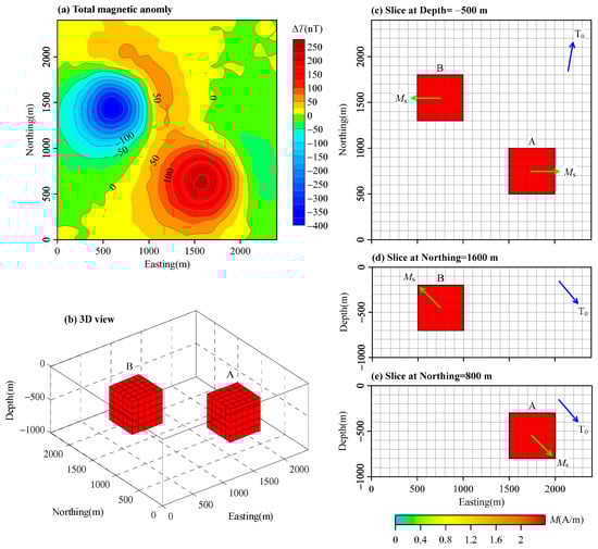
Figure 1.
Magnetic anomaly data and the spatial distribution of the combined cube models: (a) the simulated magnetic anomaly data, mixed by Gaussian random noise with a standard deviation of 3 nT; (b) 3D view of the combined cube models; (c) horizontal slice at depth = −500 m; (d) vertical slice at northing = 1600 m; (e) vertical slice at northing = 800 m.

Table 1.
Forward modeling parameters of the synthetic models.
The subspace is divided into 24 × 24 × 10 = 5760 cubic blocks with a side length of 100 m. First, we interpret the data by utilizing the L2 norm on the three orthogonal components, mx, my, and mz. Note that the smallness term and three gradient terms are all measured by the L2 norm. Figure 2 presents the inversion results, with data misfit illustrated in Figure 2a, a 3D view of magnetization intensity M > 0.2 A/m depicted in Figure 2b, and slices of the inverted models at depth = −500 m, northing = 1600 m, and northing = 800 m displayed in Figure 2c–e, respectively. The blue arrows denote the orientation of the inverted magnetization, and the black dashed lines delineate the boundaries of the true models. The results demonstrate a smooth magnetization intensity model, and the magnetization direction has continuously varying characteristics, with very poor consistency and extremely low resolution, indicating that reasonable results are impossible to acquire without appropriate constraints.
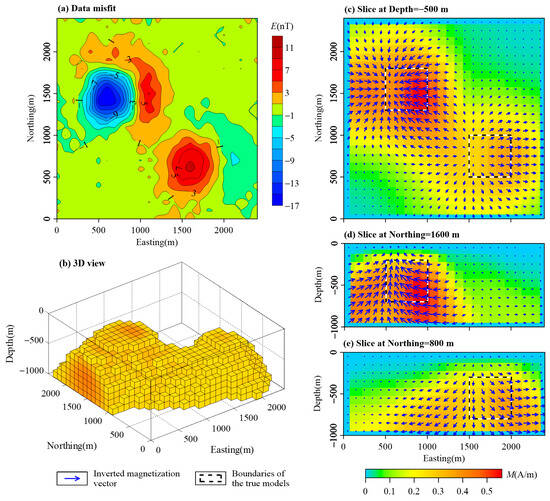
Figure 2.
Magnetization vector inversion result of the combined cube models’ data by employing the L2 norm to the three orthogonal components: (a) data misfit between the predicted and observed data; (b) 3D view of magnetization intensity M > 0.2 A/m; (c) horizontal slice at depth = −500 m; (d) vertical slice at northing = 1600 m; (e) vertical slice at northing = 800 m.
Sparse regularization operators can significantly enhance the fuzzy results of susceptibility inversion. Does applying those sparse regularization operators to the magnetization vector inversion yield the same result? Figure 3 illustrates the inversion results from the application of the L0 norm to both the model’s smallness term and gradient terms. The observed blocky structures exhibit low correlation and poor consistency in magnetization direction, diverging significantly from the true model despite being sparser than those presented in Figure 2 and providing a clearer indicator of the model’s location. This phenomenon suggests that the correlation and consistency of the magnitude and direction of the inverted magnetization vector will finally diminish when the sparse operator is only applied to the magnetization components due to the absence of correlation restrictions among them.
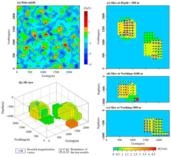
Figure 3.
Magnetization vector inversion result of the combined cube models’ data by employing the L0 norm to the three orthogonal components: (a) data misfit between the predicted and observed data; (b) 3D view of magnetization intensity M > 0.2 A/m; (c) horizontal slice at depth = −500 m; (d) vertical slice at northing = 1600 m; (e) vertical slice at northing = 800 m.
Finally, the sparse magnetization vector inversion utilizing modulus constraints is implemented on the data presented in Figure 1a. This approach applies the L0 norm to both the smallness term and gradient terms to restrict the magnetization magnitude. The inversion results in Figure 4 exhibit clear boundaries and consistent magnetization directions, which are close to the true models. Figure 5 also presents statistical diagrams of the magnitude and direction of the inverted magnetization vector derived from the three inversion results mentioned above. The inversion results based on the L2 norm exhibit dispersive magnetization magnitude and direction. In contrast, the results, based on the L0 norm, present focused models. However, applying the L0 norm to the three orthogonal components fails to obtain a reasonable magnetization direction. The proposed method achieves precise magnetization magnitude and direction through establishing correlation constraints among the components and validates its correctness.
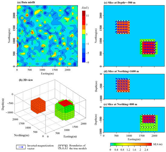
Figure 4.
Magnetization vector inversion result of the combined cube models’ data by employing the L0 norm to the magnitude: (a) data misfit between the predicted and observed data; (b) 3D view of magnetization intensity M > 0.2 A/m; (c) horizontal slice at depth = −500 m; (d) vertical slice at northing = 1600 m; (e) vertical slice at northing = 800 m.
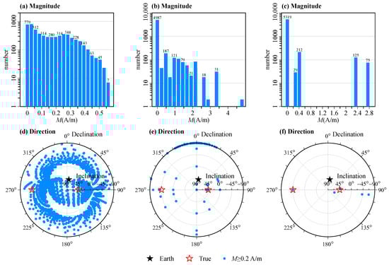
Figure 5.
Statistical diagrams of the magnitude and direction of the inverted magnetization vector from the data of combined cubic models: (a–c) bar charts of the magnetization intensity; (d–f) scatter diagrams of the magnetization direction (M ≥ 0.2 A/m); (a,d) magnetization vector inversion result by employing the L2 norm to the three orthogonal components; (b,e) magnetization vector inversion result by employing the L0 norm to the three orthogonal components; (c,f) magnetization vector inversion result by employing the L0 norm to the magnitude.
3.2. Combined Dipping Dyke Models
Previous studies [30,32] indicate that the application of sparse operators to gradient components readily produces vertical or horizontal structures and enhances image quality at corners [33]. However, it has challenges recovering sparsely inclined models. To explore the effect of magnetization vector inversion on recovering sparse and inclined structures, another model is designed under the same observation condition and the same geomagnetic field as in Figure 1. This model contains two dipping dykes in opposing directions, with the magnetization direction parallel to the models’ inclination. Table 1 details the specific forward modeling parameters of models C and D. Figure 6a presents the magnetic anomaly data ΔT (incorporating Gaussian random noise with a standard deviation of 3 nT) generated by the combined dipping dyke models.
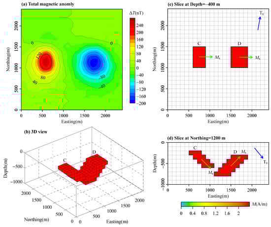
Figure 6.
Magnetic anomaly data and the spatial distribution of the combined dipping dyke models: (a) the simulated magnetic anomaly data, mixed by Gaussian random noise with a standard deviation of 3 nT; (b) 3D view of the combined dipping dyke models; (c) horizontal slice at depth = −400 m; (d) vertical slice at northing = 1200 m.
We apply the sparse magnetization vector inversion with modulus constraints to the magnetic anomaly data in Figure 6a. First, we measure the smallness term and the three gradient terms using the L0 norm. Figure 7 presents the inversion results when the L0 norm is applied to the gradient components of magnetization magnitude. The recovered magnetization direction is consistent, but the results show compact block structures, making it difficult to depict the dipping structures.
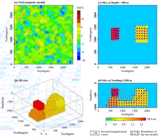
Figure 7.
Magnetization vector inversion result of the combined dipping dyke models’ data by employing the L0 norm to the gradient’s components of magnetization magnitude: (a) data misfit between the predicted and observed data; (b) 3D view of magnetization intensity M > 0.2 A/m; (c) horizontal slice at depth = −400 m; (d) vertical slice at northing = 1200 m.
To address this issue, the improved scheme proposed in Section 3.2 is adopted here. We utilize the L0 norm for the smallness term and implement the minimum gradient support stabilizer [34] for the gradient term. Thus, the sparse operator is applied to the gradient’s modulus of the magnetization magnitude. The results of the improved scheme show both sparse and tilted structures in Figure 8. Nevertheless, the consistency of magnetization direction deteriorates, exhibiting a notable difference in the tilt angle compared with the true models. Statistical diagrams of the magnitude and direction of the inverted magnetization vector in Figure 9 show that results in Figure 8 are less concentrated in magnetization direction contrasted with those in Figure 7. This indicates that employing modulus constraints alone to improve the inversion resolution for inclined structures has certain limitations.
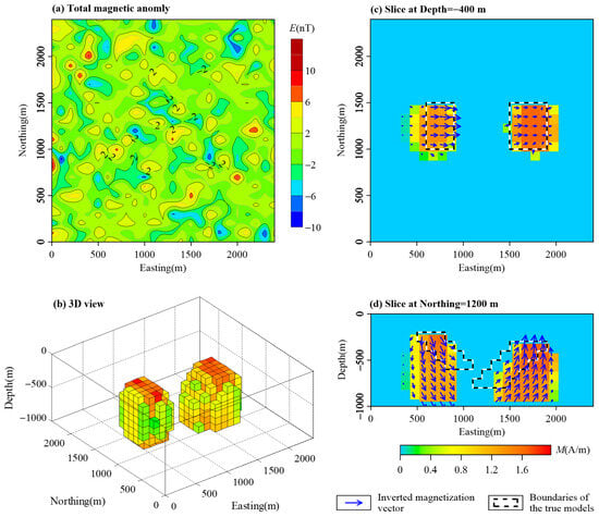
Figure 8.
Magnetization vector inversion result of the combined dipping dyke models’ data by employing the L0 norm to the gradient’s modulus of the magnetization magnitude: (a) data misfit between the predicted and observed data; (b) 3D view of magnetization intensity M > 0.2 A/m; (c) horizontal slice at depth = −400 m; (d) vertical slice at northing = 1200 m.
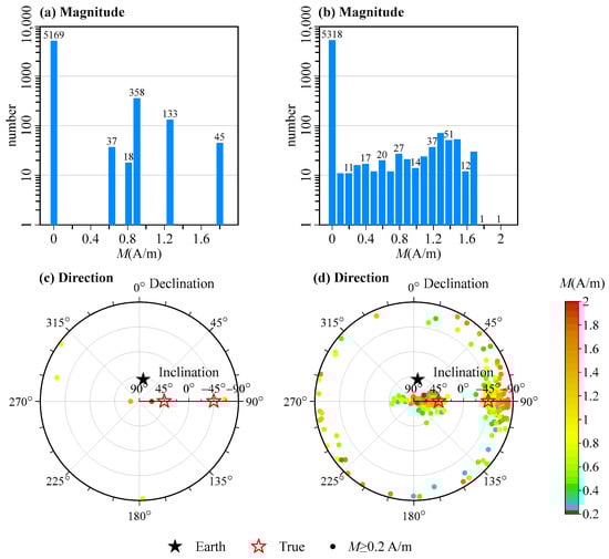
Figure 9.
Statistical diagrams of the magnitude and direction of the inverted magnetization vector from the combined dipping dyke models’ data: (a,b) bar charts of the magnetization intensity; (c,d) scatter diagrams of the magnetization direction (M ≥ 0.2 A/m); (a,c) magnetization vector inversion by applying the L0 norm to the gradient’s components of magnetization magnitude; (b,d) magnetization vector inversion by applying the L0 norm to the gradient’s modulus of the magnetization magnitude.
4. Field Example
To demonstrate the validity and applicability of the proposed approach, we apply it to the inversion of magnetic data measured over the Zaohuohexi iron-polymetallic deposit, Qinghai Province, northwest China. The magnetic survey area is located at the junction of the Northern Kunlun Magmatic Arc and the Qimantage Suture Zone [35,36]. This area is largely covered by Quaternary sediments, and most iron-polymetallic ore bodies are found in skarns at the outer contact zones of marble and granite-diorite. Magnetite has the strongest magnetism in the study area, which not only has a high susceptibility but also a strong remanent magnetization, with a Koenigsberger ratio Q = 2.1 [37]. Chalcopyrite-magnetite and mineralized skarn exhibit moderate magnetism, with a wide range of variation, making them the main interference anomalies, while rocks with moderate and weak magnetism constitute the background field [2,37].
The magnetic anomaly in the study area exhibits a regular, banded distribution in a north-west-west direction (Figure 10a), with a length of 1.6 km and a width of approximately 400 m. The anomaly is positive to the south and negative to the north, with sharp curves, high intensity (peak value reaching 1980 nT), and steep gradients, making it the strongest magnetic anomaly belt in this area. As delineated by the drill holes, the depth of the magnetic ore body gradually increases from east to west, and its thickness gradually decreases. We apply an inversion-based method [38,39] to separate the regional anomalies and local anomalies. The research region is divided into 124 × 74 × 19 = 174,344 cells in the east, north, and depth directions, with each cell having a side length of 20 m. The calculated residual magnetic anomaly in Figure 10b is then interpreted by the proposed method.
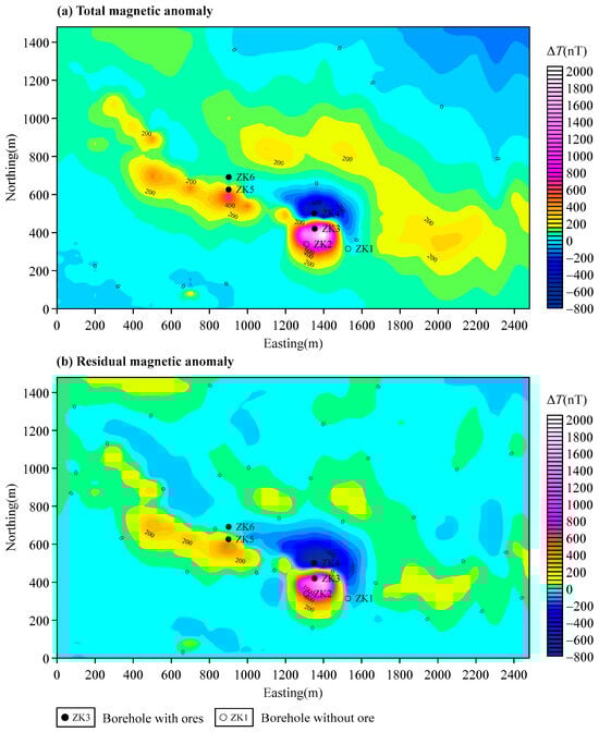
Figure 10.
(a) The magnetic anomaly of the Zaohuohexi iron-polymetallic deposit, Qinghai Province, northwest China; (b) the residual magnetic anomaly calculated by an inversion-based method.
Figure 11 shows the results of the proposed magnetization vector inversion. The distribution characteristics of the magnetization intensity are relatively simple, mainly reflecting the characteristics of moderate to strong magnetic bodies. The high-magnitude magnetization corresponds to the horizontal projection position of the magnetic ore body. The horizontal slice at depth = 2860 m in Figure 11b indicates that the magnetic anomaly in the southeast is significantly stronger than that in the northwest, which corresponds to the characteristic of the magnetite body gradually increasing in depth from east to west and becoming thinner.
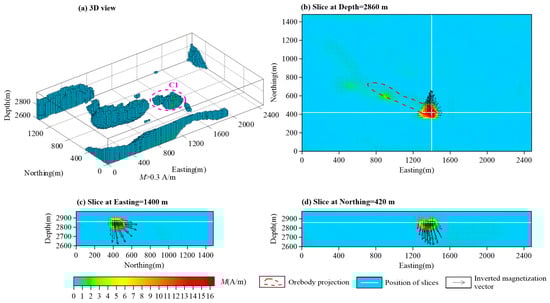
Figure 11.
Results of magnetization vector inversion from the Zaohuohexi magnetic data using the modulus constrains method: (a) 3D view of magnetization intensity M > 0.3 A/m; (b) horizontal slice at depth = 2860 m; (c) vertical slice at easting = 1400 m; (d) vertical slice at northing = 400 m.
To further analyze the results of the magnetization vector, Figure 12 summarizes the magnitude and direction of the magnetization intensity in the high magnetic area C1. Although Figure 12b shows a dispersed magnetization direction, the direction of the high magnetization intensity vector is close to the geomagnetic field direction, indicating that the remanent magnetization direction is not significantly different from the geomagnetic direction. Geological data indicate that mineralization in this region primarily occurred during the Late Triassic orogeny of the East Kunlun Orogenic Belt [40]. Since no significant tectonic movements occurred in the study area after the formation of the ore deposits, the remanent magnetization direction of the rocks did not change significantly. This result is also consistent with previous studies [2].
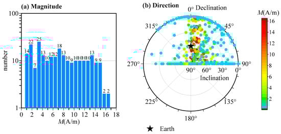
Figure 12.
Statistical diagrams of the inverted magnetization vector in the C1 area: (a) bar chart of the magnetization intensity; (b) scatter diagram of the magnetization direction.
5. Conclusions
In this study, we propose a magnetization vector inversion method based on modulus constraints. This method employs a sparse operator on the magnitude of the magnetization vector in Cartesian coordinates. Through transformation and approximation, we can obtain an explicit expression for the partial derivative of the model objective function with respect to the magnetization components. This demonstrates that it has the same form as the magnetization vector inversion in Cartesian coordinates, with the only difference in calculating the reweighted matrix. This theoretically confirms the correctness of the previously proposed compact magnetization vector inversion. The inversion of the combined cube models indicates that the modulus-based inversion can get models with clear boundaries and consistent magnetization directions by establishing correlation constraints among the magnetization components.
In addition, to obtain sparse and inclined structures, we suggest applying the sparse operator to the gradient’s modulus of the magnetization magnitude, which can alleviate the staircasing problem. Inversion of the combined dipping dyke models indicates that this improvement is beneficial for obtaining inclined structures. However, the magnetization direction becomes dispersed, as only the magnetization modulus is constrained. We think future research needs to explore the inversion method that simultaneously constrains both the magnitude and direction of the magnetization.
Finally, we apply this method to the magnetic data measured over the Zaohuohexi iron-polymetallic deposit in Qinghai Province, northwest China. The obtained magnetization vector characteristics match with the geological data, yielding results consistent with previous studies.
Author Contributions
Conceptualization, Y.O.; data curation, Y.L.; formal analysis, Y.O.; funding acquisition, J.Z. (Jie Zhang) and Y.Y.; investigation, D.J. and Y.L.; methodology, Y.O.; resources, J.Z. (Jinghong Zhai) and Z.J.; software, Y.O.; supervision, Q.L.; validation, Y.O., Y.Y. and Z.J.; visualization, J.Z. (Jinghong Zhai); writing—original draft, Y.O.; writing—review & editing, Y.O., Q.L. and D.J. All authors have read and agreed to the published version of the manuscript.
Funding
This research was funded by the National Natural Sciences Foundation of China (grant number 42104082), Central Government Surplus Research Funds for Institute of Geophysical and Geochemical Exploration (grant number JY202104), National Nonprofit Institute Research Grant of Chinese Academy of Geological Sciences (grant number JKYZD202330 and JKYQN202350), and China Geological Survey Project (grant number DD20242708).
Data Availability Statement
The original contributions presented in the study are included in the article, further inquiries can be directed to the corresponding author.
Conflicts of Interest
The authors declare no conflicts of interest.
References
- Baniamerian, J.; Liu, S.; Hu, X.; Fedi, M.; Chauhan, M.S.; Abbas, M.A. Separation of magnetic anomalies into induced and remanent magnetization contributions. Geophys. Prospect. 2020, 68, 2320–2342. [Google Scholar] [CrossRef]
- Liu, S.; Hu, X.; Zuo, B.; Zhang, H.; Geng, M.; Ou, Y.; Yang, T.; Vatankhah, S. Susceptibility and remanent magnetization inversion of magnetic data with a priori information of the Köenigsberger ratio. Geophys. J. Int. 2020, 221, 1090–1109. [Google Scholar] [CrossRef]
- Liu, S.; Fedi, M.; Hu, X.; Baniamerian, J.; Wei, B.; Zhang, D.; Zhu, R. Extracting Induced and Remanent Magnetizations From Magnetic Data Modeling. J. Geophys. Res. Solid Earth 2018, 123, 9290–9309. [Google Scholar] [CrossRef]
- Li, Y.; Sun, J.; Li, S.; Leão-Santos, M. A paradigm shift in magnetic data interpretation: Increased value through magnetization inversions. Lead. Edge 2021, 40, 89–98. [Google Scholar] [CrossRef]
- Lelievre, P.G.; Oldenburg, D.W. A 3D total magnetization inversion applicable when significant, complicated remanence is present. Geophysics 2009, 74, L21–L30. [Google Scholar] [CrossRef]
- Wang, M.Y.; Di, Q.Y. Magnetization Vector Tomography. CT Theory Appl. 2000, 9, 48–50. [Google Scholar]
- Wang, M.Y.; Di, Q.Y.; Xu, K.; Wang, R. Magnetization vector inversion equations and 2D forward and inversed model study. Chin. J. Geophys. 2004, 47, 528–534. [Google Scholar]
- Kubota, R.; Uchiyama, A. Three-dimensional magnetization vector inversion of a seamount. Earth Planets Space 2005, 57, 691–699. [Google Scholar] [CrossRef]
- Elllis, R.G.; de Wet, B.; Macleod, I.N. Inversion of Magnetic Data from Remanent and Induced Sources. ASEG Ext. Abstr. 2012, 1–4. [Google Scholar] [CrossRef]
- Liu, S.; Hu, X.; Liu, T.; Feng, J.; Gao, W.; Qiu, L. Magnetization vector imaging for borehole magnetic data based on magnitude magnetic anomaly. Geophysics 2013, 78, D429–D444. [Google Scholar] [CrossRef]
- Liu, S.; Hu, X.; Xi, Y.; Liu, T.; Xu, S. 2D sequential inversion of total magnitude and total magnetic anomaly data affected by remanent magnetization. Geophysics 2015, 80, K1–K12. [Google Scholar] [CrossRef]
- Liu, S.; Hu, X.Y.; Zhang, H.L.; Geng, M.X.; Zuo, B.X. 3D Magnetization Vector Inversion of Magnetic Data: Improving and Comparing Methods. Pure Appl. Geophys. 2017, 174, 4421–4444. [Google Scholar] [CrossRef]
- Fournier, D. A Cooperative Magnetic Inversion Method with Lp-Norm Regularization. Master’s Thesis, University of British Columbia, Vancouver, BC, Canada, 2015. [Google Scholar]
- Zhdanov, M.S.; Čuma, M.; Wilson, G.A.; Polomé, L. 3D magnetization vector inversion for SQUID-based full tensor magnetic gradiometry. In Proceedings of the 2012 SEG Annual Meeting, Las Vegas, NV, USA, 4–9 November 2012; SEG Technical Program Expanded Abstracts. pp. 1–5. [Google Scholar]
- Queitsch, M.; Schiffler, M.; Stolz, R.; Rolf, C.; Meyer, M.; Kukowski, N. Investigation of three-dimensional magnetization of a dolerite intrusion using airborne full tensor magnetic gradiometry (FTMG) data. Geophys. J. Int. 2019, 217, 1643–1655. [Google Scholar]
- Ma, G.; Zhao, Y.; Xu, B.; Li, L.; Wang, T. High-Precision Joint Magnetization Vector Inversion Method of Airborne Magnetic and Gradient Data with Structure and Data Double Constraints. Remote Sens. 2022, 14, 2508. [Google Scholar] [CrossRef]
- Meng, Q.F. Research on High Precision Joint Inversion Method of Gravity and Magnetic with Undulating Terrain. Ph.D. Thesis, Jilin University, Changchun, China, 2022. [Google Scholar]
- Wang, T.; Ma, G.; Meng, Q.; Wang, T.; Jiang, Z. Joint Inversion Method of Gravity and Magnetic Data with Adaptive Zoning Using Gramian in Both Petrophysical and Structural Domains. Surv. Geophys. 2024, 45, 1291–1330. [Google Scholar] [CrossRef]
- Ou, Y.; Feng, J. Joint magnetization vector inversion of surface and borehole magnetic data. In Proceedings of the International Workshop and Gravity, Electrical & Magnetic Methods and Their Applications, Chengdu, China, 19–22 April 2015; pp. 73–76. [Google Scholar]
- Li, Y.; Sun, J. 3D magnetization inversion using fuzzy c-means clustering with application to geology differentiation. Geophysics 2016, 81, J61–J78. [Google Scholar] [CrossRef]
- Sun, J.; Li, Y. Magnetization clustering inversion—Part 1: Building an automated numerical optimization algorithm. Geophysics 2018, 83, J61–J73. [Google Scholar] [CrossRef]
- Sun, J.; Li, Y. Magnetization clustering inversion—Part 2: Assessing the uncertainty of recovered magnetization directions. Geophysics 2019, 84, J17–J29. [Google Scholar] [CrossRef]
- Zhu, Y.; Zhdanov, M.S.; Čuma, M. Inversion of TMI data for the magnetization vector using Gramian constraints. In SEG Technical Program Expanded Abstracts 2015; Society of Exploration Geophysicists: Houston, TX, USA, 2015; pp. 1602–1606. [Google Scholar]
- Jorgensen, M.; Zhdanov, M.S.; Parsons, B. 3D Focusing Inversion of Full Tensor Magnetic Gradiometry Data with Gramian Regularization. Minerals 2023, 13, 851. [Google Scholar] [CrossRef]
- Fournier, D.; Heagy, L.J.; Oldenburg, D.W. Sparse magnetic vector inversion in spherical coordinates. Geophysics 2020, 85, J33–J49. [Google Scholar] [CrossRef]
- Ghalehnoee, M.H.; Ansari, A. Compact magnetization vector inversion. Geophys. J. Int. 2022, 228, 1–16. [Google Scholar] [CrossRef]
- Fournier, D.; Oldenburg, D.W. Inversion using spatially variable mixed ℓp norms. Geophys. J. Int. 2019, 218, 268–282. [Google Scholar] [CrossRef]
- Shi, X.; Geng, H.; Liu, S. Magnetization Vector Inversion Based on Amplitude and Gradient Constraints. Remote Sens. 2022, 14, 5497. [Google Scholar] [CrossRef]
- Xie, R.; Xiong, S.; Duan, S.; Luo, Y.; Wang, P. 2.5D magnetization vector inversion of vector magnetic data. Geophysics 2023, 88, G135–G144. [Google Scholar] [CrossRef]
- Ou, Y.; Lü, Q.; Yan, J.; Jia, D.; Li, Y. Enhancements for stabilizing functional in potential field inversion to recover sparse models with reasonable values and dipping structures. J. Appl. Geophys. 2023, 218, 105187. [Google Scholar] [CrossRef]
- Farquharson, C.G. Constructing piecewise-constant models in multidimensional minimum-structure inversions. Geophysics 2008, 73, K1–K9. [Google Scholar] [CrossRef]
- Sun, J.; Fournier, D. Understanding total variation regularization: Why can it recover dipping structures? Geophys. Prospect. 2023, 72, 424–434. [Google Scholar] [CrossRef]
- González, G.; Kolehmainen, V.; Seppänen, A. Isotropic and anisotropic total variation regularization in electrical impedance tomography. Comput. Math. Appl. 2017, 74, 564–576. [Google Scholar] [CrossRef]
- Portniaguine, O.; Zhdanov, M.S. Focusing geophysical inversion images. Geophysics 1999, 64, 874–887. [Google Scholar] [CrossRef]
- Feng, C.Y.; Zhao, Y.M.; Li, D.X.; Liu, J.N.; Xiao, Y.; Li, G.C.; Ma, S.C. Skarn Types and Mineralogical Characteristics of the Fe-Cu-polymetallic Skarn Deposits in the Qimantage Area, Western Qinghai Province. Acta Geol. Sin. 2011, 85, 1108–1115. [Google Scholar]
- Zhao, Y.M.; Feng, C.Y.; Li, D.X.; Liu, J.N.; Xiao, Y.; Yu, M.; Ma, S.C. Metallogenic setting and mineralization-alteration characteristics of major skarn Fe-polymetallic deposits in Qimantag area, western Qinghai Province. Miner. Depos. 2013, 32, 1–19. [Google Scholar]
- Ou, Y.; Feng, J.; Zhao, Y.; Jia, D.Y.; Gao, W.L. Forward modeling of magnetic data using the finite volume method with a simultaneous consideration of demagnetization and remanence. Chin. J. Geophys. 2018, 61, 4635–4646. [Google Scholar]
- Li, Y.; Oldenburg, D.W. Separation of regional and residual magnetic field data. Geophysics 1998, 63, 431–439. [Google Scholar] [CrossRef]
- Li, Z.; Yao, C. An Investigation of lp-Norm Minimization for the Artifact-Free Inversion of Gravity Data. Remote Sens. 2023, 15, 3465. [Google Scholar] [CrossRef]
- Liu, G.Y.; Zhao, Y.L.; Lin, G.; He, A.Q.; Wang, Z.S.; Li, Z. Preliminary analysis of prospecting potential in the western Zaohuohe iron polymetallic ore deposit area in eastern Kunlun belt. Miner. Explor. 2017, 8, 559–567. [Google Scholar]
Disclaimer/Publisher’s Note: The statements, opinions and data contained in all publications are solely those of the individual author(s) and contributor(s) and not of MDPI and/or the editor(s). MDPI and/or the editor(s) disclaim responsibility for any injury to people or property resulting from any ideas, methods, instructions or products referred to in the content. |
© 2025 by the authors. Licensee MDPI, Basel, Switzerland. This article is an open access article distributed under the terms and conditions of the Creative Commons Attribution (CC BY) license (https://creativecommons.org/licenses/by/4.0/).