Abstract
Indoor scenes often contain complex layouts and interactions between objects, making 3D modeling of point clouds inherently difficult. In this paper, we design a divide-and-conquer modeling method considering the structural differences between indoor walls and internal objects. To achieve semantic understanding, we propose an effective 3D instance segmentation module using a deep network Indoor3DNet combined with super-point clustering, which provides a larger receptive field and maintains the continuity of individual objects. The Indoor3DNet includes an efficient point feature extraction backbone with good operability for different object granularity. In addition, we use a geometric primitives-based modeling approach to generate lightweight polygonal facets for walls and use a cross-modal registration technique to fit the corresponding instance models for internal objects based on their semantic labels. This modeling method can restore correct geometric shapes and topological relationships while maintaining a very lightweight structure. We have tested the method on diverse datasets, and the experimental results demonstrate that the method outperforms the state-of-the-art in terms of performance and robustness.
1. Introduction
The automatic 3D reconstruction of indoor scenes from point clouds has become increasingly popular for a wide range of applications, such as augmented/virtual reality, robotic navigation, and building maintenance [1,2]. However, it is a complex task hindered by uneven density, noise, and incompleteness of data, whether captured by laser scanners or RGB-D cameras [3]. Specifically, it is challenging to accurately reconstruct the shapes of objects like furniture, as the gaps and noise in point clouds significantly compromise the reliability of existing methods.
Conventional explicit data-driven surface modeling methods struggle to reconstruct complete shapes when encountering regions with large missing data. Therefore, many methods are developed using grammatical rules or pattern matching [4,5,6], and object-level modeling results are achieved by leveraging prior knowledge of indoor environments. The latest advances in 3D deep learning have facilitated the understanding of 3D indoor environments and automatic 3D modeling [1,7]. Some semantics-supported methods aim to match and align Computer-Aided Design (CAD) models with the detected objects [8,9,10,11], leading to parametric models.
Although some classification algorithms [12,13,14,15] have achieved considerable accuracy and precision, the segmentation of indoor point clouds remains challenging overall. Point clouds, unlike the structured 2D image data, are inherently irregular and unordered, presenting a challenge for the direct application of Convolutional Neural Networks (CNNs) designed for grid-like data [16]. Moreover, the computational demands for processing extensive point clouds are notably high. One of our primary objectives is to propose a new deep learning network for indoor scene parsing, which assigns different instance labels to point clouds, such as tables, chairs, walls, etc. This network aims to enhance the precision of point cloud classification and enable advanced capabilities, such as instance segmentation.
On the other hand, indoor scenes usually exhibit different granularity levels, which refer to their visual structural disparities. Indoor walls typically have a lower granularity level, characterized by larger, flatter, and more continuous structures. In contrast, interior objects have a higher granularity level due to their intricate shapes and spatial arrangements. We propose a practical hybrid method that applies distinct strategies to walls and internal objects, considering these differences in their granularity levels. Using our semantic parsing framework, we segment the input point cloud into two parts, i.e., exterior walls (including the wall, floor, and ceiling) and interior objects (furniture). Room walls are depicted using polygonal surfaces, while internal furniture is modeled using corresponding CAD models from a predefined library.
Different from previous CAD model-based methods that pose the models in the inferred 3D bounding boxes [1,17,18], we design a cross-modal registration method (mesh to point cloud registration) to address the scale and orientation issues in the model fitting. The proposed approach aims to achieve semantic richness and topological correctness. The final merged models lead to a comprehensive representation of the indoor environment and allow for easy editing, meeting a wide range of application needs, such as architectural design and simulation of the indoor environment.
Most existing methods either build the main structure of the rooms [19,20,21,22,23,24] or generate mesh models for the interior objects [1,9,18], lacking a modeling method that can maintain different granularities. The main contributions of this paper are as follows:
- The Indoor3DNet is developed as a novel 3D neural network that utilizes positional encoding to perform semantic segmentation on indoor point clouds. It effectively captures multi-granular features using positional encoding and skip connection structures. The connection structures are likely used to enhance the network’s ability to capture detailed and contextual information from indoor point clouds, thereby improving the accuracy of semantic segmentation;
- A super-point clustering strategy is integrated into the instance segmentation module. It allows the module to obtain more accurate and continuous instance labels on the point clouds, promoting a divide-and-conquer modeling approach that accounts for the structural disparities between walls and interior objects;
- A hybrid modeling approach is created for the generation of lightweight semantic indoor models. The modeling module allows for a clean and compact reconstruction of the room walls and enables the parametric rendering of interior objects.
2. Related Work
Research in indoor modeling from point clouds involves a range of techniques and methodologies. In the following, we review the relevant literature from three aspects.
2.1. Geometric-Prior Driven Modeling
Early surface modeling methods only yield a skin-like surface by extracting iso-surfaces. Typically, these surface models can approximate entire point clouds but lack semantic understanding, failing to differentiate between components such as walls and clutter. In addition, conventional meshing methods often degrade in the presence of noisy and partial scans [25].
Given the vertical orientation of indoor walls, 3D wall structures can be transformed into 2D line drawings. Consequently, some line feature-based methods utilize line frameworks to aid in wall model construction [21,22,23]. To produce more regular room structures, early methods decompose point clouds into horizontal slices, identify walls as line segments, and work in 2D before merging into 3D [26,27]. Using some regularization constraints, these algorithms are effective for environments with mainly orthogonal or parallel features. Chen et al. [19] introduced a scalable indoor modeling technique that optimizes linear element segmentation in space through horizontal slicing and binary energy minimization methods. Although these methods are adept at representing vertical walls through the detection of intersecting planes, the disconnected line segments may contain substantial noise and detail and lead to fault structures.
Another group of methods relies on basic geometric elements and prior shape grammars to approximate room outlines. The renowned RANSAC algorithm [28] has been widely used in various methods to generate planar hypotheses for building architecture [29]. In the study by Ikehata et al. [20], a scene is conceptualized as a structure graph. The reconstruction process is facilitated by the application of a structure grammar that serves to define and enforce the admissible transformation rules governing the evolution of the graph. Wei et al. [30] proposed a robust method for segmenting planar 3D reconstruction and completion from large-scale unstructured point clouds. Their approach leverages the Manhattan assumption to extract a simplified model of buildings from point clouds, effectively reconstructing and completing missing or incomplete data while maintaining planar consistency. Although such models are concise, they may overlook certain complex details. The Polyfit modeling method [31] is designed to create polynomial models that fit planar hypotheses on the input point clouds by solving a binary optimization function. The method can obtain a very concise result of the exterior surface of the building. However, the fitting accuracy is highly dependent on the desired precision level, and achieving higher accuracy may require additional constraints or more refined data preprocessing. These approaches mainly concentrate on permanent wall structures, omitting consideration of complex indoor furniture.
2.2. Semantic-Prior Driven Modeling
By training models on extensive labeled data, deep learning-based methods strive to accurately predict 3D reconstructions from incomplete point cloud inputs. This allows object-level analysis even when working with partial scans by integrating instance segmentation information, involving approaches such as volume-based methods [32], mesh-based methods [1], and graph-based methods [11].
Some prominent methodologies leverage neural networks to learn implicit representations or shape priors of 3D objects, such as Mesh R-CNN [33] and GeoRec [1]. This capability facilitates the direct reconstruction of 3D geometry from point cloud data. Using the structural features of RGB-D scan data, certain methods can employ voxels or grids to achieve Convolutional Neural Network model designs. For instance, RevealNet [34] is a fully convolutional 3D network that joins color and geometry feature learning to detect independent objects and infer their complete geometric shapes. Similarly, RfD-Net [17] uses RGB-D data to conduct the indoor semantic reconstruction, aiming to simultaneously achieve 3D object detection and mesh prediction.
An alternative approach is to use CAD models of certain objects to replace the point cloud data and construct the model [11,35,36]. These methods decompose intricate geometries into more manageable instance forms, thereby enabling a more accurate representation of missing structures in terms of geometric fidelity. Nan et al. [5] leverage geometric and symmetry descriptors to retrieve the most similar models from a 3D model library. Izadinia et al. [20] align CAD models with predefined 3D room boundaries and employ object proposals to refine the accuracy of the reconstruction process. In current deep learning methods, ensuring model accuracy in feature extraction and modeling across different scales continues to be a persistent challenge.
2.3. Deep Learning-Based Indoor Parsing
Deep learning-based instance segmentation is critical for semantic prior-driven reconstruction, and there has been more interest in deep learning for 3D point cloud classification and segmentation [12,13,37]. The early methods typically project point clouds into bird’s eye view (BEV) [38] or range/depth images [39] and then process them using 2D neural network techniques. These strategies are not suitable for intricate indoor scenes. Designing the learning modules for 3D voxels can be achieved by directly extending the well-studied 2D CNN networks to 3D [40,41,42]. The parameter count of these networks would increase cubically due to the additional dimension compared with the 2D data structure. Moreover, graph neural network-based methods can organize convolution operations in point clouds with graph structures [43]. To leverage local geometric structures, Shen et al. [44] employed kernel correlation for feature learning, followed by calculating the affinity between these kernels and the specific neighborhood points.
By directly processing point clouds, certain 3D neural networks, such as PointNet [45], PointNet++ [46], KPConv [47], and RandLA-Net [48], are effective due to their capacity to comprehend spatial information without depending on predefined grid structures. The advancement of multi-layer perceptron (MLP) for point feature extraction has been demonstrated in these models. To better capture the local and global features of large datasets, such methods employ techniques including farthest point sampling (FPS), random sampling (RS), local feature aggregation (LFA), etc. SemanticFlow [14] introduces a sparse-frame-supervised segmentation network, utilizing a small number of fully annotated frames instead of partially annotated points within all frames. SFL-NET [49] employs SFConv to reduce redundancy in convolutional filters, thereby enhancing the efficiency of local feature extraction.
The outstanding performance of Transformers [50] has also extended to the realm of point cloud data processing. Point transformer networks like PointNN [51], PCT [52], and Stratified Transformer [53] have expanded the semantic segmentation capability with increased receptive field and the ability to recognize the interaction between features. However, their high computational requirements hinder the application in large scenes. More recently, Luo et al. [54] proposed the Dense Dual-Branch Cross Attention Network (D2CAN) for semantic segmentation of large-scale point clouds. Their approach integrates Local Context Deep Perception (LCDP) and Global Feature Pyramid Dense Fusion (GFDF) modules to enhance local feature extraction and global context modeling, achieving state-of-the-art performance. However, the dense feature fusion and attention mechanisms may introduce higher computational costs. In summary, point cloud semantic segmentation remains a challenging and computationally expensive task. This paper proposes a method that follows deep learning-based instance segmentation and semantic prior-driven approaches as part of its contribution.
3. Method
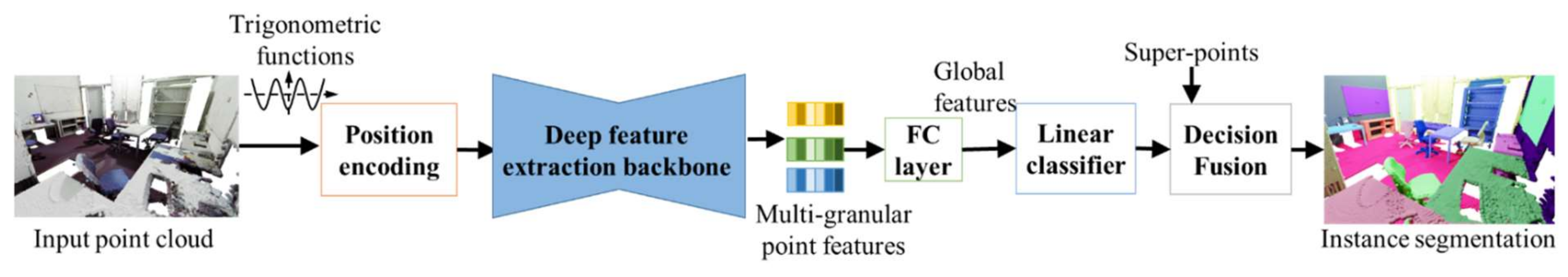
As illustrated in Figure 1, our pipeline comprises two primary modules: (1) an indoor parsing module based on a deep semantic labeling network (i.e., Indoor3DNet) and (2) a hybrid modeling module (i.e., Hybrid-Modeler) responsible for building mesh models.
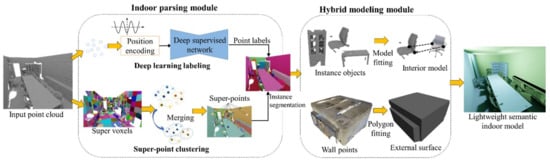
Figure 1.
Overview of the modeling method. The indoor parsing module uses a deep supervised semantic labeling network and super-point information to predict the semantic labels of each point and segment them into different instances. Subsequently, the hybrid modeling module estimates geometric primitives from the predefined instances and reconstructs the exterior walls and interior objects separately.
- (1)
- Indoor parsing module: Indoor3DNet first adopts a position-encoding strategy to promote the feature extraction of points, utilizing trigonometric functions. Subsequently, a point feature extraction backbone is designed based on an encoder–decoder structure to extract multi-granular features. The output is the semantic labels for each point. A parallel routine incrementally constructs super-point structures to cover larger homogeneous regions. Every point within a super-point inherits homogenous class distributions, thereby assigning a clustering label for each point. By merging the deep semantic labels and super-point information, the algorithm effectively segments the point cloud into distinct instances;
- (2)
- Hybrid modeling module: The hybrid-modeler aims to extract geometric primitives from the predefined instance classes and independently reconstruct the walls and interior objects. The walls are represented using a combination of polygon primitives, resulting in a lightweight model. In contrast, the interior objects are aligned with their respective semantic CAD models to generate a detailed reconstruction. The final output is a lightweight semantic model that represents indoor scenes in a compact format.
3.1. Indoor Parsing Module
3.1.1. Indoor3DNet
As illustrated in Figure 2, the Indoor3DNet is a deep semantic labeling network, which first encodes the point position into high-dimensional vectors by concatenating the embeddings of , , and axes. Then, the network progressively aggregates the spatial local features through a multi-stage hierarchical FPS, k Nearest Neighbors (k-NN), and MLP.

Figure 2.
Workflow of the proposed Indoor3DNet.
Position encoding. The 3D position encodes for point clouds and is estimated by trigonometric functions, inspired by the methods described in PointNN [51] and PCT [52]. For each point within the point cloud , its , , and coordinates are embedded separately by sine and cosine functions and then their embeddings are concatenated to form high-dimensional feature vectors, .
where denotes the dimension of the feature, , and the notation represents a value from one of the dimensions , , or . The wavelengths form a geometric series ranging from to .
The inherent properties of trigonometric functions enable the encoded feature vector to effectively capture relative position information between different points. The spatial relation of two points can be depicted by a dot product of their embeddings. In addition, for any fixed offset , can be represented as a linear function of , which facilitates the extraction of high-frequency information and the capture of fine-grained structural changed in 3D shapes.
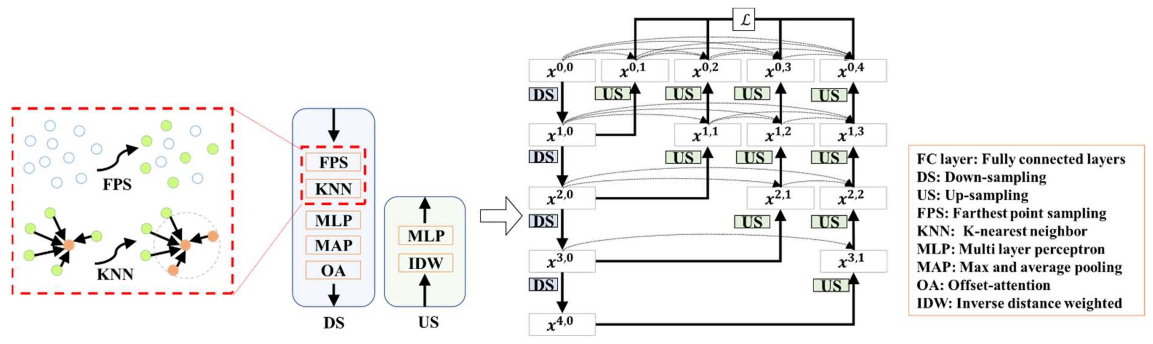
Deep feature extraction sub-network. Figure 3 illustrates the deep supervised encoder–decoder sub-network. By adopting the encoder–decoder architecture [55], we expand the network by adding more intermediate nodes and incorporating skip connections between each of these nodes. At the end of each down-sampling (DS) block, an offset-attention (OA) mechanism, as originally proposed in PCT [52], is incorporated. Additionally, deep supervision is employed to enable gradients to propagate back to the intermediate nodes, facilitating faster and more effective convergence of the model. This, in turn, allows the model to flexibly adjust network depth through pruning, thus achieving a balance between accuracy and efficiency.
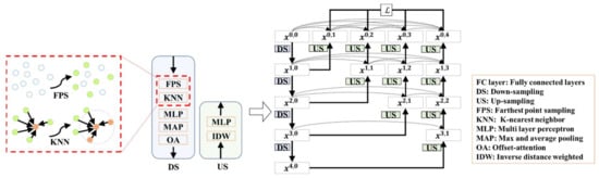
Figure 3.
The deeply-supervised encoder–decoder network for multi-granular feature extraction.
We use a 4-layer network structure to boost accuracy further when computational resources are available. Each DS block conducts local feature extraction as local information aggregation, starting from FPS and followed by -NN to obtain local 3D region sets.
As the proposed network directly processing points, the FPS is adopted to reduce the density of the point cloud while preserving its overall shape and structural features. Then, the -NN operator clusters the closest points neighbour points around the sampled points to construct local region sets. Additionally, we apply MLP for each local 3D region to extract local features, followed by an aggregation step that employs both max and average pooling, denoted as
where denotes the estimate of the maximum value, represents the formula for calculating the average value, and is the coefficient. Notice that max pooling may discard a considerable amount of local information by only selecting the maximum feature. Average pooling can also attenuate key features. By combining max and average pooling, we have substantially aggregated local information, enhancing the feature representation.
After the pooling process, the features are refined through OA, which is estimated based on the input feature of the self-attention (SA) block and its output feature . The result of OA is the offset between the input features and the output features of the enhanced SA, as follows:
where represents the continuous operations of the Linear, BatchNorm, and ReLU layers. Then, the up-sampling (US) block uses the same inverse distance interpolation as in PointNet [45] for interpolation, followed by global feature learning through an MLP.
Loss function. In the encoder–decoder sub-network, each down-sample layer has a corresponding up-sampled layer that has a same size of the input point cloud, as the nodes , , , and show in Figure 3. The loss function for each layer employs a cross-entropy measure, and the overall loss function is defined as a weighted aggregation of the individual losses from the decoder stages.
where represents the loss of the layer . In this context, is the one-hot encoded label vector that represents the true labels of the data, where each class is represented by a binary vector with a 1 in the position of the correct class and 0 elsewhere. represents the predicted label probability vector generated by the model, indicating how likely each class is for a given input. represents the point within the layer, while represents the total number of points within .
At the top layer nodes, i.e., , , , and , we predict the semantic label of each point, and they maintain segmentation capabilities. The skip connections allow the network to propagate gradient information to the earlier layers.
Similar concepts are also employed in RFFS-Net [56]. RFFS-Net targets airborne laser scanning (ALS) data, using multi-scale receptive field fusion and stratification to address complex structures and scale variations. It incorporates Dilated Graph Convolution (DGConv) and Annular Dilated Convolution (ADConv) to capture multi-scale features, integrates features via the DAGFusion module, and optimizes classification with Multi-level Receptive Field Aggregation Loss (MRFALoss).
In contrast, Indoor3DNet is designed for indoor point clouds, incorporating positional encoding to capture spatial relationships. It employs FPS and -NN for feature extraction, followed by aggregation using MAP. The loss function is a weighted sum of cross-entropy losses from decoder stages. In summary, RFFS-Net excels in handling complex ALS data through multi-scale fusion, while Indoor3DNet leverages positional encoding and precise local feature extraction for indoor classification.
3.1.2. Super-Point Guided Instance Segmentation
Growth of super-points. To further generate instance segmentation, we use a modified Voxel Cloud Connectivity Segmentation (VCCS) [57] method to perform the over-segmentation on the input point cloud. The coordinates of the patch centroids serve as the coordinates of the corresponding super voxels, while the normal vectors of these super voxels are determined based on the points within the patches. Subsequently, a region-growing algorithm is applied in the context of super voxel growth, incrementally expanding the super-points to create larger homogenous regions, i.e., super-points.
The growth of super-points is constrained by the criteria: if the spatial distance and feature similarity between neighboring super-points fall within a pre-defined threshold, they are merged. This merging process is crucial in the propagation of labels, ensuring that all points within the same super-point are assigned a uniform clustering label, thereby providing a higher-level representation of the scene.
Final instance segmentation. A decision fusion process is applied to integrate two types of labels (from the deep network and the super-point clustering) to generate final instance labels that are closely aligned with the distribution of real-world objects. The decision fusion process involves a comparative analysis between the semantic and clustering labels for each point, with subsequent label adjustments based on the intersection coverage between these labels.
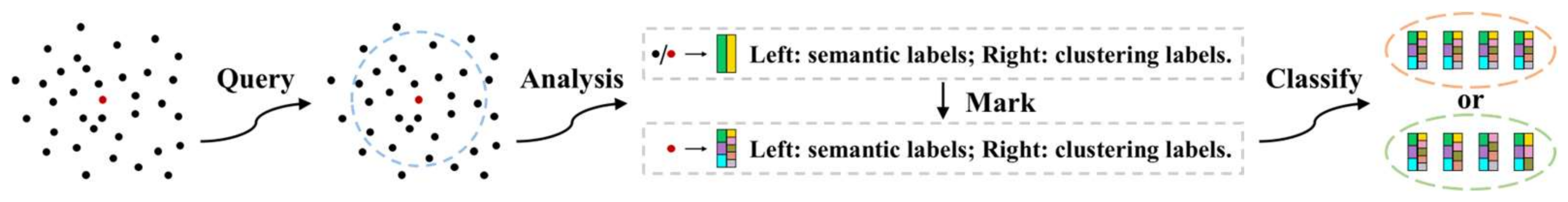
Specifically, we designed an algorithm based on heuristic strategies to bring the adjustment of semantic and clustering labels for each point closer to their true values in a bottom-up manner by combining local analysis and global optimization. This algorithm focuses on the boundaries where discrepancies occur between semantic and clustering labels in 3D space. First, we marked and classified points, as shown in Figure 4. The algorithm starts by selecting k nearest neighbors of each point in its local neighborhood using a ball query method. Then, it compares the labels of these neighboring points to search for differences. If the semantic labels are varied while the clustering labels are uniform, or vice versa, the point is marked to reflect this discrepancy.
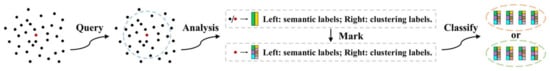
Figure 4.
Illustration of the schematic representation of marking and classification rules.
The marking method is expressed as follows: (left: all semantic labels in the local neighborhood, right: all instance labels in the local neighborhood). After traversing all points, we will merge some semantic/clustering labels according to pre-defined decision rules. We merge and classify points with the same mark, as well as those points where one side demonstrates a containment relationship in terms of their markings.
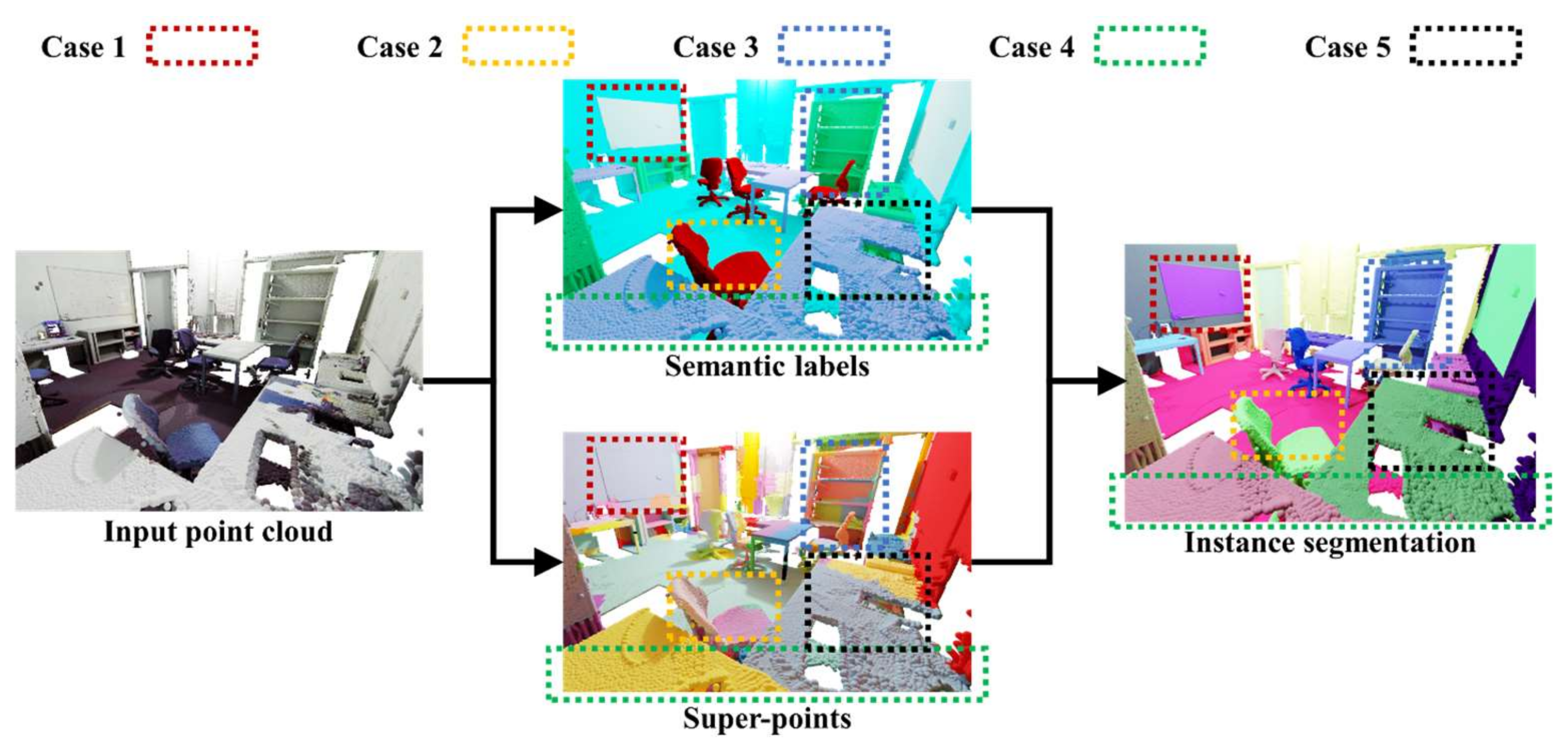
Then, for points classified into one category, we conduct decision fusion analysis on the clustering regions they are in. An example of instance segmentation is shown in Figure 5. If there are the same clustering labels but different semantic labels in the region (Case 1), we choose to believe the semantic boundary and modify the instance labels of these points according to the semantic boundary. If there are different clustering but same semantics in the region, we conduct decision analysis based on the number of classified points and the number of points in the clustering region they are in. If the number of classified points is less than a pre-defined threshold (Case 2), or the number of clusters in the clustering region is greater than a pre-defined threshold (Case 3), we choose to believe the semantic boundary and modify the instance labels of these points according to the semantic boundary. On the contrary of Case 2 and Case 3 (Case 4), we choose to believe the clustering boundary and modify the instance labels of these points according to the clustering boundary. If there are different semantics and clustering labels in the region (Case 5), we choose to believe the semantic boundary and modify the instance labels of these points according to the semantic boundary.
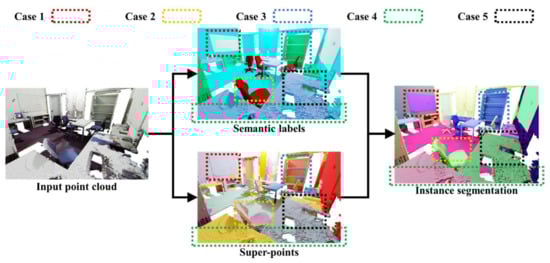
Figure 5.
A visual result of the proposed algorithm for indoor instance segmentation. Different colors represent different instance segmentation.
3.2. Hybrid Modeling Module
After instance segmentation, the locations of walls and interior objects are determined, so the hybrid-modeler can be executed by replacing the scatted point clouds with regular 3D shapes, as shown in Figure 6.
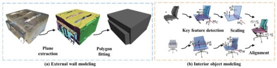
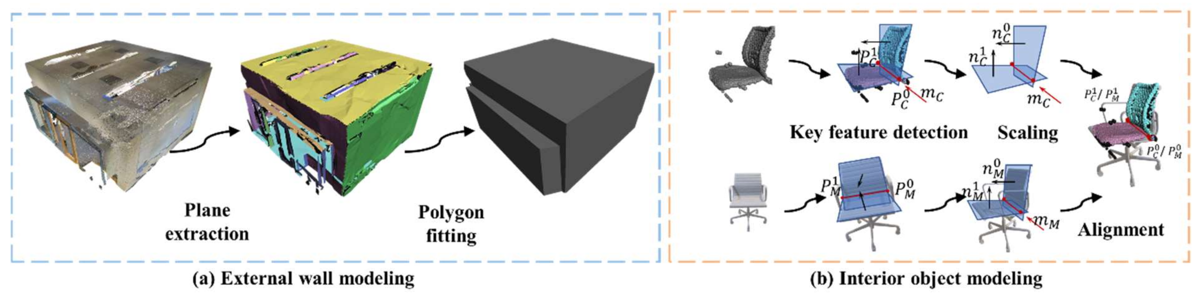
Figure 6.
Illustration of the method in the hybrid modeling module.
External wall modeling using the Polyfit algorithm. The walls of rooms are typically composed of straightforward planes. According to our statistics, these structures make up a large part of the point cloud, accounting for approximately 70% of the entire scene. Based on the classic Polyfit [31] algorithm, we perform plane fitting on points that are labeled as walls, including the ceiling, floor, and walls. As we can exclude interior object points during the extraction of planar elements, the Polyfit [31] method demonstrates effective performance on wall points, thereby achieving lightweight and ideal wall structures.
Interior object modeling based on cross-modal registration. For interior objects, we arrange the CAD models in the predefined model library to replace the segmented objects based on their semantic labels. A cross-modal registration algorithm is proposed to find the ideal registration of 3D models to the object locations.
The cross-modal registration method involves the computation of a 7 DoF (degree of freedom) transformation matrix, as outlined in Formula (6), to align the instance point cloud with its corresponding model.
where represents the feature points extracted from the model, while represents the feature points extracted from the instance point cloud. The variable denotes the scale factor, represents the rotation matrix, and represents the translation. The solution process can be outlined as follows.
We define some geometric feature-based patterns for the typical furniture in the model library, such as a sofa, chair, bookcase, and table. For instance, each chair contains two planes and an intersecting line segment, and each table or cabinet contains three orthogonal planes from an observation angle, etc. Based on the labels of the instance point cloud and the preset geometry feature patterns, we can find matching features between the model and the point cloud. The following is an explanation of feature estimate and transformation for objects such as chairs. The estimate processer is similar for other furniture as well.
Taking the chair model as an example, we initially extract geometric primitives, including some main planes of furniture and their intersecting line segments. The endpoints of these line segments serve as pivotal key points. To ensure unique matching, the normal vectors of the planes are oriented consistently toward the space encompassing the centroid. Furthermore, the direction vector of the intersection line segments is established by computing the cross-product of the normal vectors associated with the perpendicular and horizontal planes.
Subsequently, the transform scale for the CAD model is determined based on the length of the corresponding intersection line segment. The rotation matrix is solved based on the angle constraint between the direction vector of the intersection line segment and the corresponding plane normal vector. The translation vector is computed using the endpoints of the intersection line segment.
where and represent the th feature points extracted from the model and the object point cloud. and represent the unit direction vectors of the intersection line segments derived from the model and the point cloud. Additionally, and are the unit normal vectors of extracted planes. In order to achieve consistency in direction, the value of is assigned based on the role of the feature point within the direction vector: if the feature point is the starting endpoint, then ; conversely, if it is the ending endpoint, then . The subscript is assigned based on the orientation of the plane: if the plane is vertical, then ; if the plane is horizontal, then .
Based on the correspondences of the above features, the 7Dof transformation between the model and the point cloud can be estimated. Other furniture items are also aligned using similar predefined pattern features to estimate the registration transformation parameters, thereby matching the models to the positions. At the end, by integrating the wall surfaces and interior objects, the indoor models are completed. Due to the highly structured representation used in modeling both the walls and internal objects of the house, the data volume of the entire model is very lightweight, and the model result has the ability for semantic analysis and easy editing.
3.3. Implementation Details
We conducted training for all neural networks on a workstation with an Intel Core i9-13900K CPU, 64 GB RAM, and an NVIDIA GeForce RTX, 4090 GPU. For the Indoor3DNet, we use the Adam optimizer with an initial learning rate of , trained for 200 epochs with 70% step decay every 10 epochs, and set the batch size to 32. Specifically, the output dimension of the position encoding layer is set to 144. For FPS, we use ratios of 1/4, 1/16, 1/64, and 1/256 and select 16 nearest neighbour points for the -NN parameter. The dimensions of different depth feature layers are 96, 256, 512, and 1024, respectively.
We conducted experiments on different datasets. These datasets were collected using different sensor devices, including RGB-D camera and LiDAR. In our study, the object classes in the original dataset have been simplified by merging categories, such as beams, columns, and windows merged into walls. The indoor modeling categories of our classification network include walls, tables, chairs, sofas, bookcases, and boards.
S3DIS [58]: It is a comprehensive benchmark dataset of large 3D indoor spaces captured by Matterport RGB-D camera. It covers 272 rooms in 6 areas with diverse scenes and totals 695,878,620 points. Points range from 500,000 to 2.5 million per room, each with coordinates and color attributes.
UZH 3D Dataset [59]: It consists of 40 rooms and 13 environments, focusing on complex office and residential spaces. Captured with a Faro Focus3D LiDAR scanner, it features multi-scan composites with 10 million points each, combining multiple stations for comprehensive data, including coordinates, color, and intensity.
NUAA3D: Our dataset contains one office and four conference rooms captured with a Leica BLK360 LiDAR scanner in the university. It provides detailed point clouds with an average of 20 million points per scene, scanned from multiple angles to minimize occlusions, and includes coordinates, color, and intensity for each point. This dataset serves the algorithm for precision analysis of the models and is also used for assessing the transfer capabilities of deep neural networks.
Table 1 shows the information of the test data used in our paper, including the number of points and the total number of objects.

Table 1.
Information for the dataset example.
4. Results and Discussion
4.1. Reconstruction Results
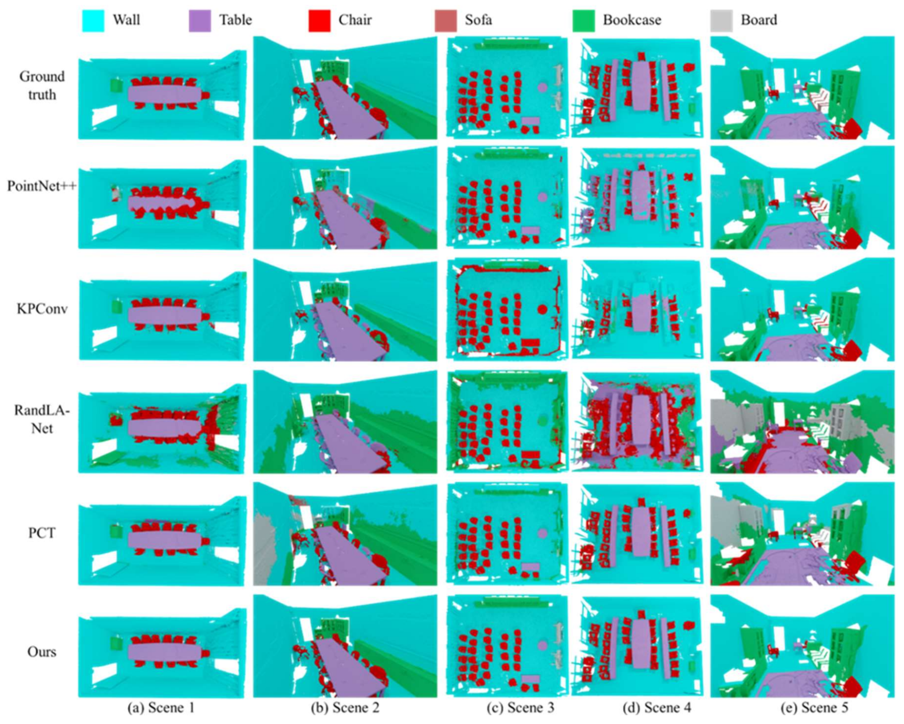
The indoor semantic parsing results include point labeling results and the further instance segmentation results. We conducted tests on the S3DIS dataset [58] and the UZH dataset [59]. The method has been compared with other methods, including PointNet++ [46], KPConv [47] and RandLA-Net [48], and PCT [52]. The visualization results of semantic labeling for the point clouds are shown in Figure 7, where the dashed boxes indicate some areas with serious incorrect labels. The visual results show that our results are more in line with the ground truth. Even in the case of a small sample, our method can effectively segment complex categories. This capability is attributed to the network’s effective semantic recognition of high-frequency information and its ability to aggregate local features, thereby achieving accurate segmentation inferences.
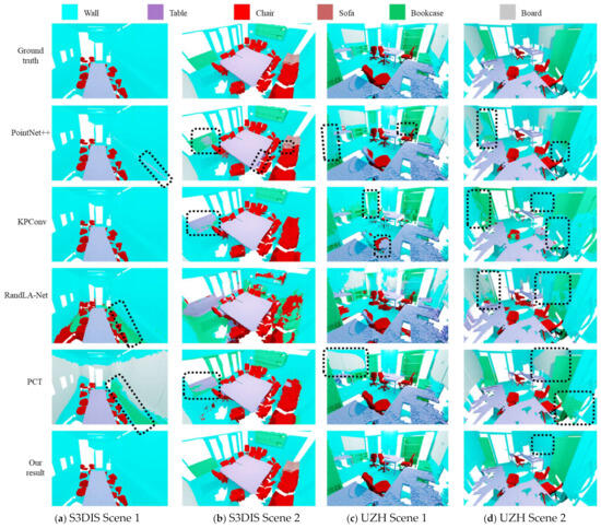
Figure 7.
Visualization of the point labeling results on the S3DIS datasetand UZH 3D dataset.
The evaluation metrics for the indoor parsing module include overall accuracy (OA), mean accuracy (mAcc), and mean intersection over union (mIoU). The mathematical formulas can be expressed as follows:
where the terms , , , and represent true positives, false positives, true negatives, and false negatives, respectively. The variable represents the number of categories in the datasets.
For the modeling module, where the ground truth is often missing, a common metric for assessing the quality of reconstructed models is to estimate the root mean square (RMS) error of the surface fitting, as follows below:
where is the shortest distance from a point to the mesh model and represents the number of points in the point cloud.
The quantitative results related to Figure 7 are presented in Table 2 and Table 3, indicating that our method achieved high scores on both datasets. On the S3DIS dataset [58] (RGB-D points), our method achieved an mIoU of 73.5%, marking an improvement of 9.1% over the second methods, i.e., PointNet++ [46]. Similarly, our method has also achieved excellent performance on the UZH 3D dataset [59], which is LiDAR point clouds. Our method outperforms other methods in terms of OA and mIoU. This can be attributed to our position encoding module, which will be discussed in the ablation experiments.
Table 2.
Reconstruction results on the S3DIS dataset.
Table 3.
Reconstruction results on the UZH 3D dataset.
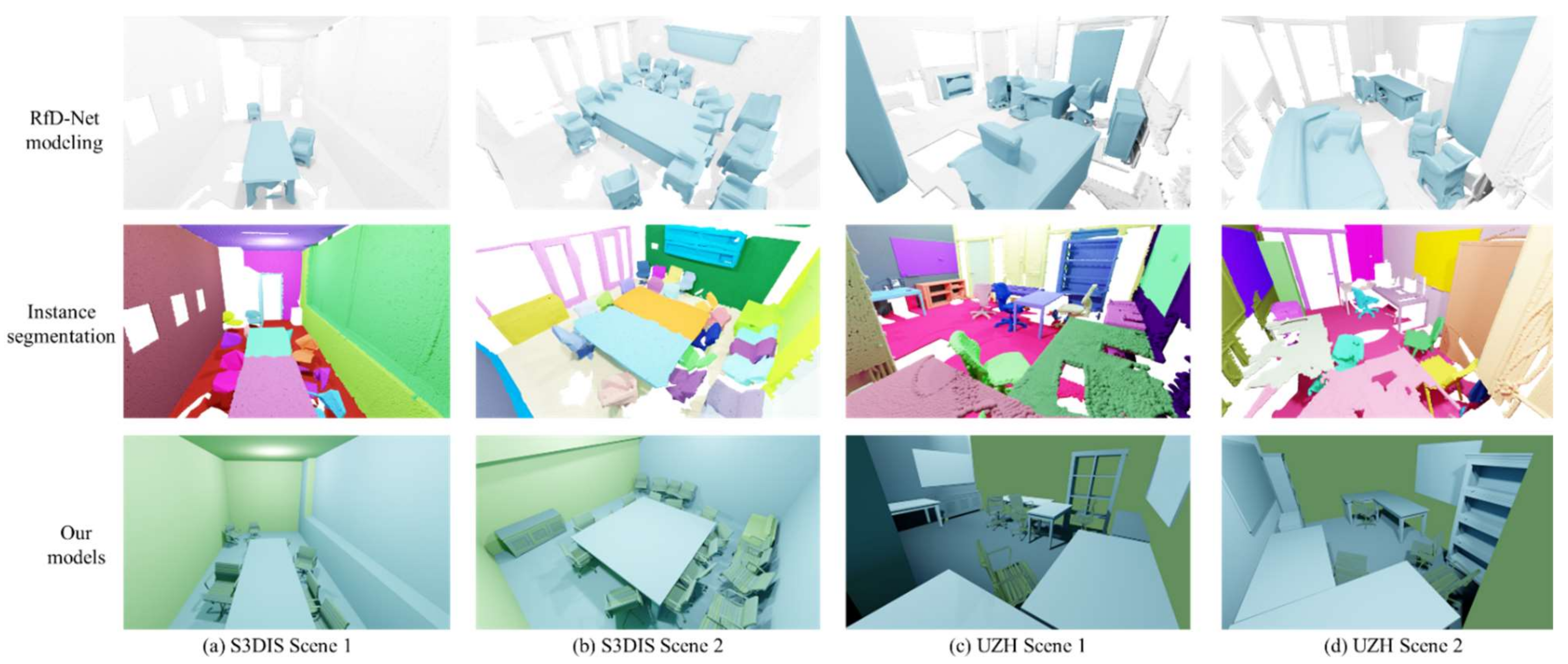
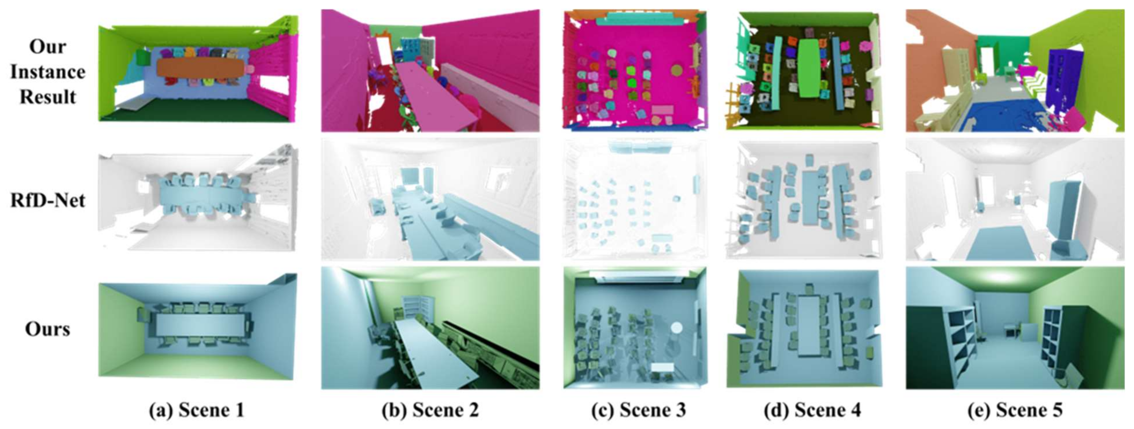
We also compared the final reconstruction results of our method with those of RfD-Net [17]. As shown in Figure 8, our reconstruction results (third row) better capture the real scene with instance segmentation results (second row). The first row illustrates the object reconstructions of RfD-Net [17], which often generates multiple model outputs for a single instance object and frequently leaves a substantial number of instances unreconstructed.
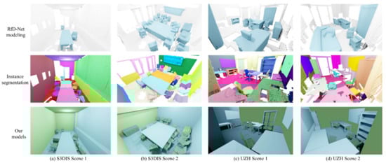
Figure 8.
Visualization of reconstruction results on the S3DIS dataset and UZH 3D dataset.
The quantitative analysis of the final models is conducted using the RMS metric, with the statistics summarized in Table 4. The RMS values of our model are all below 0.12 m, whereas the value of RfD-Net [17] is 1 m. This indicates that our model demonstrates superior performance.
Table 4.
Reconstruction of RMS on the S3DIS dataset and the UZH 3D dataset.
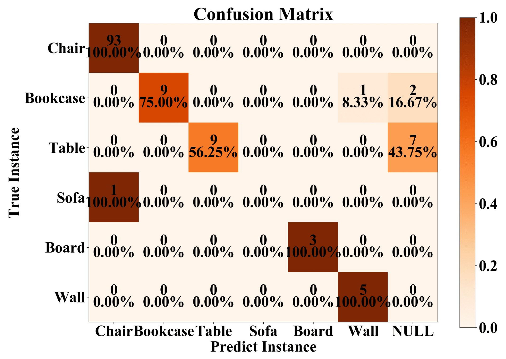
To further assess the completeness of the reconstructed instances, we present a confusion matrix of our result, as shown in Figure 9. The horizontal axis represents the predicted instance results (successfully reconstructed), while the vertical axis represents the actual instances.
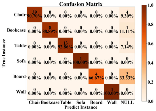
Figure 9.
Confusion matrix on the S3DIS dataset and UZH 3D dataset. The NULL indicates that the instance cannot be successfully reconstructed.
4.2. More Results on the NUAA3D Dataset
We also use the NUAA3D dataset for testing; the visualizations are depicted in Figure 10, and the modeling results are depicted in Figure 11. To further assess the completeness of the reconstruction results, as shown in Figure 12, a confusion matrix comparing the reconstruction results of our method and RfD-Net is presented [17]. Furthermore, we performed quantitative analysis on the reconstruction results of our method and RfD-Net [17], with the primary evaluation metric being the RMS, and the results are summarized in Table 5. The RMS of our method’s reconstruction results is within 0.06 m, outperforming RfD-Net [17], which achieves 0.9 m.
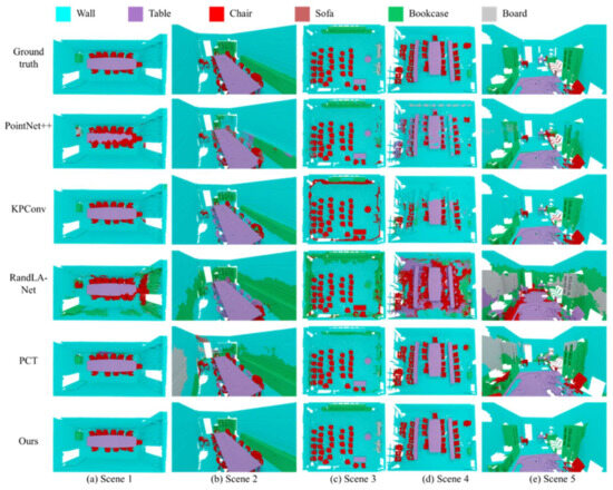
Figure 10.
Visualization of point labeling results on the NUAA3D dataset.

Figure 11.
Visualization of reconstruction results on the NUAA3D dataset.

Figure 12.
Confusion matrix on the NUAA3D dataset. The NULL indicates that the instance cannot be successfully reconstructed.
Table 5.
Reconstruction of RMS on the NUAA3D dataset.
4.3. Ablation Study
4.3.1. Impact of Specific Blocks
In our semantic parsing module, several network blocks are used, including FPS + -NN, PosEmb, DS, OA, and the decision fusion (DF). To elucidate the individual contributions of each process to the model’s performance, we executed a series of ablation studies by constructing network model variants named A1, A2, A3, and A4, as listed in Table 6. We observe that there is an improvement in the transition from model A1 to A2, which can be largely attributed to the incorporation of positional encoding. This encoding captures both the absolute and relative spatial orientations of the points, along with the implicit high-frequency components, thereby significantly improving the model’s ability to distinguish points across various categories.
Table 6.
Ablation study.
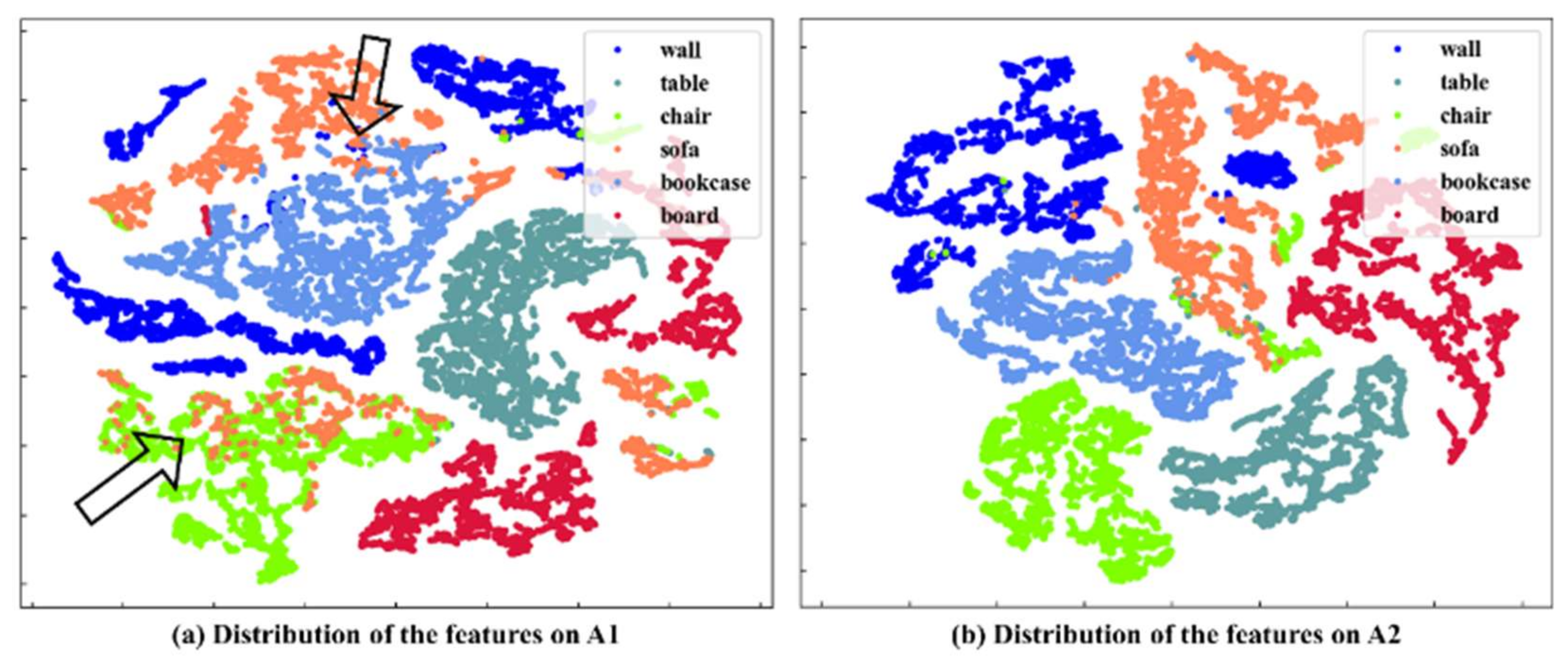
Furthermore, we compare and discuss the feature distributions before and after position encoding, as illustrated in Figure 13. As indicated by the arrows in the feature distribution maps, there is inter-class overlap among features before position encoding, such as the sofa class overlapping with the chair and table classes, indicating limited discriminative capability. After position encoding, the inter-class overlap of features is greatly mitigated, and the intra-class distances become more compact, leading to clearer feature distinction.

Figure 13.
Feature distribution before and after position encoding. Arrows in (a) indicate inter-class overlap before position encoding.
4.3.2. Impact of Parameter Settings
Furthermore, we analyze the impact of the value and the selection of position encoding dimension (PosE_dim) on the model. As shown in Table 7, the highest OA score is achieved at “”, which is 0.9% higher than “”. In terms of mIoU scores, “” performs at 63.2%, marking an improvement of 1.7% over “”. Given the minimal performance disparity between “” and “” and considering the computational efficiency, we opt for the lesser computational load of “”. The comparison of position encoding dimension selection is depicted in Table 8, where a dimension of 144 yields the highest OA and mIoU.
Table 7.
Ablation study of .
Table 8.
Ablation study on the impact of position encoding dimension.
In addition, we have also analyzed the parameter count for different layers of our network, with the input tensor dimensions of [9, 4096], as shown in Table 9.
Table 9.
Ablation study on the parameter count for different layers of Indoor3DNet. A comparison with PointNet [45].
4.4. Limitation
We acknowledge that our current approach has limitations. First, small objects, such as wall decorations and table tools, may still be overlooked. Additionally, the accuracy of internal object models is limited by CAD fitting methods, as they rely on the diversity of offline model libraries. Nevertheless, the method only models one room at a time, and the modeling results can capture the indoor scene structure in a concise and comprehensive manner.
5. Conclusions and Future Work
This paper introduces a semantic modeling method for indoor scenes that is proficient in learning geometric feature representations from a variety of data sources. The indoor parsing module integrates the labeling results of Indoor3DNet and the super-points clustering information with decision fusion to provide instance segmentation, which is crucial for indoor semantic 3D reconstruction. Furthermore, we use a hybrid modeling approach that leverages geometric primitives to generate lightweight internal wall models and to align CAD models of indoor objects based on the determined instance labels. The experimental results on multiple datasets demonstrate the superior performance and robustness of the proposed method in semantic segmentation and reconstruction of indoor scenes. In future work, we plan to explore the modeling capability of this method in multiple rooms, including corridors and stairs.
Author Contributions
Conceptualization, M.L. (Minglei Li) and M.L. (Mingfan Li); methodology, M.L. (Minglei Li) and M.L. (Mingfan Li); software, M.L. (Mingfan Li); validation, M.L. (Minglei Li); formal analysis, M.L. (Minglei Li), M.L. (Minglei Li), M.L. (Min Li), and L.X.; investigation, M.L. (Mingfan Li) and M.L. (Minglei Li); writing—original draft preparation, M.L. (Minglei Li) and M.L. (Mingfan Li); writing—review and editing, M.L. (Mingfan Li) and M.L. (Minglei Li); visualization, M.L. (Mingfan Li); supervision, M.L. (Minglei Li); project administration, M.L. (Minglei Li); funding acquisition, M.L. (Minglei Li). All authors have read and agreed to the published version of the manuscript.
Funding
This work was funded by the National Natural Science Foundation of China: Grant 42271343.
Data Availability Statement
The data that support the findings of this study are available on request from the corresponding author.
Conflicts of Interest
The authors declare no conflicts of interest.
References
- Huan, L.; Zheng, X.; Gong, J. GeoRec: Geometry-enhanced semantic 3D reconstruction of RGB-D indoor scenes. ISPRS J. Photogramm. Remote Sens. 2022, 186, 301–314. [Google Scholar] [CrossRef]
- Rhee, T.; Petikam, L.; Allen, B.; Chalmers, A. Mr360: Mixed reality rendering for 360 panoramic videos. IEEE Trans. Vis. Comput. Graph. 2017, 23, 1379–1388. [Google Scholar] [CrossRef] [PubMed]
- Kim, Y.M.; Ryu, S.; Kim, I.-J. Planar Abstraction and Inverse Rendering of 3D Indoor Environments. IEEE Trans. Vis. Comput. Graph. 2021, 27, 2992–3006. [Google Scholar] [CrossRef] [PubMed]
- Cui, Y.; Li, Q.; Yang, B.; Xiao, W.; Chen, C.; Dong, Z. Automatic 3-D Reconstruction of Indoor Environment with Mobile Laser Scanning Point Clouds. IEEE J. Sel. Top. Appl. Earth Obs. Remote Sens. 2019, 12, 3117–3130. [Google Scholar] [CrossRef]
- Nan, L.; Xie, K.; Sharf, A. A search-classify approach for cluttered indoor scene understanding. ACM Trans. Graph. 2012, 31, 137:1–137:10. [Google Scholar] [CrossRef]
- Zheng, Y.; Weng, Q. Model-Driven Reconstruction of 3-D Buildings Using LiDAR Data. IEEE Geosci. Remote Sens. Lett. 2015, 12, 1541–1545. [Google Scholar] [CrossRef]
- Zhang, Y.; Xu, W.; Tong, Y.; Zhou, K. Online structure analysis for real-time indoor scene reconstruction. ACM Trans. Graph. 2015, 34, 159:1–159:13. [Google Scholar] [CrossRef]
- Avetisyan, A.; Dahnert, M.; Dai, A.; Savva, M.; Chang, A.X.; NieBner, M. Scan2CAD: Learning CAD Model Alignment in RGB-D Scans. In Proceedings of the IEEE/CVF Conference on Computer Vision and Pattern Recognition (CVPR), Long Beach, CA, USA, 15–20 June 2019; pp. 2609–2618. [Google Scholar]
- Li, M.; Li, M.; Xu, L.; Wei, M. Hybrid 3D reconstruction of indoor scenes integrating object recognition. Remote Sens. 2024, 16, 638. [Google Scholar] [CrossRef]
- Poux, F.; Neuville, R.; Nys, G.-A.; Billen, R. 3D Point Cloud Semantic Modelling: Integrated Framework for Indoor Spaces and Furniture. Remote Sens. 2018, 10, 1412. [Google Scholar] [CrossRef]
- Wang, T.; Wang, Q.; Ai, H.; Zhang, L. Semantics-and-Primitives-Guided Indoor 3D Reconstruction from Point Clouds. Remote Sens. 2022, 14, 4820. [Google Scholar] [CrossRef]
- Li, Y.; Li, X.; Zhang, Z.; Shuang, F.; Lin, Q.; Jiang, J. DenseKPNET: Dense Kernel Point Convolutional Neural Networks for Point Cloud Semantic Segmentation. IEEE Trans. Geosci. Remote Sens. 2022, 60, 1–13. [Google Scholar] [CrossRef]
- Chen, D.; Zhang, L.; Mathiopoulos, P.T.; Huang, X. A Methodology for Automated Segmentation and Reconstruction of Urban 3-D Buildings from ALS Point Clouds. IEEE J. Sel. Top. Appl. Earth Observ. Remote Sens. 2014, 7, 4199–4217. [Google Scholar] [CrossRef]
- Zhao, J.; Huang, W.; Wu, H.; Wen, C.; Yang, B.; Guo, Y.; Wang, C. SemanticFlow: Semantic Segmentation of Sequential LiDAR Point Clouds from Sparse Frame Annotations. IEEE Trans. Geosci. Remote Sens. 2023, 61, 1–11. [Google Scholar] [CrossRef]
- Wang, M.; Lyu, X.; Li, Y.; Zhang, F. VR content creation and exploration with deep learning: A survey. Comput. Vis. Media. 2020, 6, 3–28. [Google Scholar] [CrossRef]
- Guo, Y.; Wang, H.; Hu, Q.; Liu, H.; Liu, L.; Bennamoun, M. Deep Learning for 3D Point Clouds: A Survey. IEEE Trans. Pattern Anal. Mach. Intell. 2021, 43, 4338–4364. [Google Scholar] [CrossRef]
- Nie, Y.; Hou, J.; Han, X.; Niesner, M. RfD-Net: Point Scene Understanding by Semantic Instance Reconstruction. In Proceedings of the IEEE/CVF Conference on Computer Vision and Pattern Recognition (CVPR), Nashville, TN, USA, 20–25 June 2021; pp. 4606–4616. [Google Scholar]
- Zhang, C.; Cui, Z.; Zhang, Y.; Zeng, B.; Pollefeys, M.; Liu, S. Holistic 3D Scene Understanding from a Single Image with Implicit Representation. In Proceedings of the IEEE/CVF Conference on Computer Vision and Pattern Recognition (CVPR), Nashville, TN, USA, 20–25 June 2021; pp. 8829–8838. [Google Scholar]
- Chen, D.; Wan, L.; Hu, F.; Li, J.; Chen, Y.; Shen, Y.; Peethambaran, J. Semantic-aware room-level indoor modeling from point clouds. Int. J. Appl. Earth Obs. Geoinf. 2024, 127, 103685. [Google Scholar] [CrossRef]
- Ikehata, S.; Yang, H.; Furukawa, Y. Structured Indoor Modeling. In Proceedings of the IEEE International Conference on Computer Vision (ICCV), Santiago, Chile, 13–16 December 2015; pp. 1323–1331. [Google Scholar]
- Lin, Y.; Wang, C.; Chen, B.; Zai, D.; Li, J. Facet Segmentation-Based Line Segment Extraction for Large-Scale Point Clouds. IEEE Trans. Geosci. Remote Sens. 2017, 55, 4839–4854. [Google Scholar] [CrossRef]
- Ochmann, S.; Vock, R.; Klein, R. Automatic reconstruction of fully volumetric 3D building models from oriented point clouds. ISPRS J. Photogramm. Remote Sens. 2019, 151, 251–262. [Google Scholar] [CrossRef]
- Tao, W.; Xiao, Y.; Wang, R.; Lu, T.; Xu, S. A Fast Registration Method for Building Point Clouds Obtained by Terrestrial Laser Scanner via 2-D Feature Points. IEEE J. Sel. Top. Appl. Earth Observ. Remote Sens. 2024, 17, 9324–9336. [Google Scholar] [CrossRef]
- Zhao, B.; Hua, X.; Yu, K.; Xuan, W.; Chen, X.; Tao, W. Indoor Point Cloud Segmentation Using Iterative Gaussian Mapping and Improved Model Fitting. IEEE Trans. Geosci. Remote Sens. 2020, 58, 7890–7907. [Google Scholar] [CrossRef]
- Sulzer, R.; Marlet, R.; Vallet, B.; Landrieu, L. A Survey and Benchmark of Automatic Surface Reconstruction from Point Clouds. arXiv 2024, arXiv:2301.13656. [Google Scholar] [CrossRef]
- Xiao, J.; Furukawa, Y. Reconstructing the world’s museums. In Proceedings of the European Conference on Computer Vision (ECCV), Florence, Italy, 7–13 October 2012; pp. 668–681. [Google Scholar]
- Oesau, S.; Lafarge, F.; Alliez, P. Indoor scene reconstruction using feature sensitive primitive extraction and graph-cut. ISPRS J. Photogramm. Remote Sens. 2014, 90, 68–82. [Google Scholar] [CrossRef]
- Schnabel, R.; Wahl, R.; Klein, R. Efficient RANSAC for Point-Cloud Shape Detection. Comput. Graph. Forum. 2007, 26, 214–226. [Google Scholar] [CrossRef]
- Li, M.; Wonka, P.; Nan, L. Manhattan-World Urban Reconstruction from Point Clouds. In Proceedings of the Computer Vision–ECCV 2016: 14th European Conference, Amsterdam, The Netherlands, 11–14 October 2016; pp. 54–69. [Google Scholar]
- Wei, J.; Wu, H.; Yue, H.; Jia, S.; Li, J.; Liu, C. Automatic Extraction and Reconstruction of a 3D Wireframe of an Indoor Scene from Semantic Point Clouds. Int. J. Digit. Earth. 2023, 16, 3239–3267. [Google Scholar] [CrossRef]
- Nan, L.; Wonka, P. PolyFit: Polygonal Surface Reconstruction from Point Clouds. In Proceedings of the IEEE International Conference on Computer Vision (ICCV), Venice, Italy, 22–29 October 2017; pp. 2372–2380. [Google Scholar]
- Li, C.; Guan, T.; Yang, M.; Zhang, C. Combining data-and-model-driven 3D modelling (CDMD3DM) for small indoor scenes using RGB-D data. ISPRS J. Photogramm. Remote Sens. 2021, 180, 1–13. [Google Scholar] [CrossRef]
- Gkioxari, G.; Johnson, J.; Malik, J. Mesh R-CNN. In Proceedings of the IEEE/CVF International Conference on Computer Vision (ICCV), Seoul, Republic of Korea, 27 October–2 November 2019; pp. 9784–9794. [Google Scholar]
- Hou, J.; Dai, A.; Nießner, M. RevealNet: Seeing Behind Objects in RGB-D Scans. In Proceedings of the IEEE/CVF Conference on Computer Vision and Pattern Recognition (CVPR), Seattle, WA, USA, 13–19 June 2020; pp. 2095–2104. [Google Scholar]
- Bansal, A.; Russell, B.; Gupta, A. Marr Revisited: 2D-3D Alignment via Surface Normal Prediction. In Proceedings of the IEEE/CVF Conference on Computer Vision and Pattern Recognition (CVPR), Las Vegas, NV, USA, 27–30 June 2016; pp. 5965–5974. [Google Scholar]
- Izadinia, H.; Shan, Q.; Seitz, S. IM2CAD. In Proceedings of the IEEE/CVF Conference on Computer Vision and Pattern Recognition (CVPR), Honolulu, HI, USA, 21–26 July 2017; pp. 2422–2431. [Google Scholar]
- Zhang, H.; Xu, F. MixedFusion: Real-Time Reconstruction of an Indoor Scene with Dynamic Objects. IEEE Trans. Vis. Comput. Graph. 2018, 24, 3137–3146. [Google Scholar] [CrossRef]
- Cortinhal, T.; Tzelepis, G.; Erdal Aksoy, E. SalsaNext: Fast, Uncertainty-Aware Semantic Segmentation of LiDAR Point Clouds. In Proceedings of the Advances in Visual Computing: 15th International Symposium, ISVC 2020, San Diego, CA, USA, 5–7 October 2020; pp. 207–222. [Google Scholar]
- Chen, X.; Ma, H.; Wan, J.; Li, B.; Xia, T. Multi-view 3D Object Detection Network for Autonomous Driving. In Proceedings of the IEEE/CVF Conference on Computer Vision and Pattern Recognition (CVPR), Honolulu, HI, USA, 21–26 July 2017; pp. 6526–6534. [Google Scholar]
- Riegler, G.; Ulusoy, A.; Geiger, A. OctNet: Learning Deep 3D Representations at High Resolutions. In Proceedings of the IEEE/CVF Conference on Computer Vision and Pattern Recognition (CVPR), Honolulu, HI, USA, 21–26 July 2017; pp. 6620–6629. [Google Scholar]
- Tchapmi, L.; Choy, C.; Armeni, I.; Gwak, J.; Savarese, S. SEGCloud: Semantic Segmentation of 3D Point Clouds. In Proceedings of the 2017 International Conference on 3D Vision (3DV), Qingdao, China, 10–12 October 2017; pp. 537–547. [Google Scholar]
- Wang, P.; Liu, Y.; Guo, Y.; Sun, C.; Tong, X. O-CNN: Octree-based convolutional neural networks for 3D shape analysis. ACM Trans. Graph. 2017, 36, 72:1–72:11. [Google Scholar] [CrossRef]
- Wang, Y.; Sun, Y.; Liu, Z.; Sarma, S.; Bronstein, M.; Solomon, J. Dynamic Graph CNN for Learning on Point Clouds. ACM Trans. Graph. 2019, 38, 146:1–146:12. [Google Scholar] [CrossRef]
- Shen, Y.; Feng, C.; Yang, Y.; Tian, D. Mining Point Cloud Local Structures by Kernel Correlation and Graph Pooling. In Proceedings of the IEEE/CVF Conference on Computer Vision and Pattern Recognition (CVPR), Salt Lake City, UT, USA, 18–23 June 2018; pp. 4548–4557. [Google Scholar]
- Qi, C.; Su, H.; Kaichun, M.; Guibas, L. PointNet: Deep Learning on Point Sets for 3D Classification and Segmentation. In Proceedings of the IEEE/CVF Conference on Computer Vision and Pattern Recognition (CVPR), Honolulu, HI, USA, 21–26 July 2017; pp. 77–85. [Google Scholar]
- Qi, C.; Yi, L.; Su, H.; Guibas, L. PointNet++: Deep hierarchical feature learning on point sets in a metric space. In Proceedings of the Advances in Neural Information Processing Systems (NeurIPS), Long Beach, CA, USA, 4–9 December 2017; pp. 5105–5114. [Google Scholar]
- Thomas, H.; Qi, C.; Deschaud, J.; Marcotegui, B.; Goulette, F.; Guibas, L. KPConv: Flexible and Deformable Convolution for Point Clouds. In Proceedings of the IEEE/CVF International Conference on Computer Vision (ICCV), Seoul, Republic of Korea, 27 October–2 November 2019; pp. 6410–6419. [Google Scholar]
- Hu, Q.; Yang, B.; Xie, L.; Rosa, S.; Guo, Y.; Wang, Z.; Trigoni, N.; Markham, A. RandLA-Net: Efficient Semantic Segmentation of Large-Scale Point Clouds. In Proceedings of the IEEE/CVF Conference on Computer Vision and Pattern Recognition (CVPR), Seattle, WA, USA, 13–19 June 2020; pp. 11105–11114. [Google Scholar]
- Li, X.; Zhang, Z.; Li, Y.; Huang, M.; Zhang, J. SFL-NET: Slight Filter Learning Network for Point Cloud Semantic Segmentation. IEEE Trans. Geosci. Remote Sens. 2023, 61, 1–14. [Google Scholar] [CrossRef]
- Vaswani, A.; Shazeer, N.; Parmar, N.; Uszkoreit, J.; Jones, L.; Gomez, A.; Kaiser, Ł.; Polosukhin, I. Attention is all you need. In Proceedings of the Advances in Neural Information Processing Systems (NeurIPS), Long Beach, CA, USA, 4–9 December 2017; pp. 6000–6010. [Google Scholar]
- Zhang, R.; Wang, L.; Wang, Y.; Gao, P.; Li, H.; Shi, J. Starting from Non-Parametric Networks for 3D Point Cloud Analysis. In Proceedings of the IEEE/CVF Conference on Computer Vision and Pattern Recognition (CVPR), Vancouver, BC, Canada, 17–24 June 2023; pp. 5344–5353. [Google Scholar]
- Guo, M.; Cai, J.; Liu, Z.; Mu, T.; Martin, R.; Hu, S. PCT: Point cloud transformer. Comput. Vis. Media. 2021, 7, 187–199. [Google Scholar] [CrossRef]
- Lai, X.; Liu, J.; Jiang, L.; Wang, L.; Zhao, H.; Liu, S.; Qi, X.; Jia, J. Stratified Transformer for 3D Point Cloud Segmentation. In Proceedings of the IEEE/CVF Conference on Computer Vision and Pattern Recognition (CVPR), New Orleans, LA, USA, 18–24 March 2022; pp. 8500–8509. [Google Scholar]
- Luo, Z.; Zeng, Z.; Tang, W.; Wan, J.; Xie, Z.; Xu, Y. Dense Dual-Branch Cross Attention Network for Semantic Segmentation of Large-Scale Point Clouds. IEEE Trans. Geosci. Remote Sens. 2024, 62, 1–16. [Google Scholar] [CrossRef]
- Zhou, Z.; Siddiquee, M.; Tajbakhsh, N.; Liang, J. UNet++: Redesigning Skip Connections to Exploit Multiscale Features in Image Segmentation. IEEE Trans. Med. Imaging. 2020, 39, 1856–1867. [Google Scholar] [CrossRef] [PubMed]
- Mao, Y.; Chen, K.; Diao, W.; Sun, X.; Lu, X.; Fu, K.; Weinmann, M. Beyond Single Receptive Field: A Receptive Field Fusion-and-Stratification Network for Airborne Laser Scanning Point Cloud Classification. ISPRS J. Photogramm. Remote Sens. 2022, 188, 45–61. [Google Scholar] [CrossRef]
- Papon, J.; Abramov, A.; Schoeler, M.; Wörgötter, F. Voxel Cloud Connectivity Segmentation-Supervoxels for Point Clouds. In Proceedings of the IEEE/CVF Conference on Computer Vision and Pattern Recognition (CVPR), Portland, Oregon, 25–27 June 2013; pp. 2027–2034. [Google Scholar]
- Armeni, I.; Sener, O.; Zamir, A.; Jiang, H.; Brilakis, I.; Fischer, M.; Savarese, S. 3D Semantic Parsing of Large-Scale Indoor Spaces. In Proceedings of the IEEE/CVF Conference on Computer Vision and Pattern Recognition (CVPR), Las Vegas, NV, USA, 27–30 June 2016; pp. 1534–1543. [Google Scholar]
- University of Zurich: UZH 3D Dataset. 2014. Available online: https://www.ifi.uzh.ch/en/vmml/research/datasets.html (accessed on 1 December 2024).


Disclaimer/Publisher’s Note: The statements, opinions and data contained in all publications are solely those of the individual author(s) and contributor(s) and not of MDPI and/or the editor(s). MDPI and/or the editor(s) disclaim responsibility for any injury to people or property resulting from any ideas, methods, instructions or products referred to in the content. |
© 2025 by the authors. Licensee MDPI, Basel, Switzerland. This article is an open access article distributed under the terms and conditions of the Creative Commons Attribution (CC BY) license (https://creativecommons.org/licenses/by/4.0/).