Article

Spatial Downscaling of Satellite Sea Surface Wind with Soft-Sharing Multi-Task Learning

1
School of Computer Science, China University of Geosciences, Wuhan 430074, China
2
Wuhan Digital Engineering Institute, Wuhan 430205, China
3
College of Meteorology and Oceanography, National University of Defense Technology, Changsha 410073, China
4
Fiberhome Telecommunication Technologies Co., Ltd., Wuhan 430073, China
*
Author to whom correspondence should be addressed.
Remote Sens. 2025, 17(4), 587; https://doi.org/10.3390/rs17040587
Submission received: 20 December 2024 / Revised: 3 February 2025 / Accepted: 7 February 2025 / Published: 8 February 2025

Abstract

:
Sea surface wind (SSW) plays a pivotal role in numerous research endeavors pertaining to meteorology and oceanography. SSW fields derived from remote sensing have been widely applied; however, regional and local studies require higher-spatial-resolution SSW fields to identify refined details. Most of the existing studies based on deep learning have constructed mappings from low-resolution inputs to high-resolution downscaled estimates. However, these methods have failed to capture the relationships between multiple variables as revealed by physical processes. Therefore, this paper proposes a spatial downscaling approach for satellite sea surface wind that employs soft-sharing multi-task learning. Sea surface temperature and water vapor are included as auxiliary variables for SSW, considering the close correlation revealed by physical principles and data availability. The spatial downscaling of auxiliary variables is designed as an auxiliary task and integrated into a multi-task learning network with generative adversarial network and dual regression structures. The proposed multi-task downscaling network achieves flexible parameter sharing and information exchange between tasks through a soft-sharing mechanism and bridge modules. Comprehensive experiments were conducted with WindSat SSW products at 0.25° from Remote Sensing Systems. The experimental results validate the outstanding downscaling capability of the proposed methodology with respect to precision in comparison with buoy measurements and reconstruction quality.

1. Introduction

Sea surface wind (SSW), one of the fundamental drivers of ocean momentum, plays a crucial role in Earth system science research [1]. The significance of precise and timely SSW observations extends across multiple domains, including marine environmental monitoring, numerical weather prediction (NWP), search and rescue missions, transportation, and wind energy assessment [2]. While SSW data can be collected through in situ observations from monitoring stations, buoys, and ships, these traditional measurements, despite their accuracy, face several limitations, such as sparse sampling density, restricted spatial coverage, uneven geographical distribution, and vulnerability to adverse weather conditions. Remote sensing (RS) instruments, including scatterometers, radiometers, altimeters, and spaceborne synthetic aperture radar (SAR), have emerged as valuable tools for SSW observation in meteorological and oceanographic applications [3]. Nevertheless, the relatively coarse spatial resolution of current SSW data products presents a significant challenge in capturing fine-scale variability, particularly for regional and local studies requiring detailed analysis [4,5].
Spatial downscaling represents a critical methodology for deriving high-resolution (HR) fine-scale data from low-resolution (LR) large-scale conditions, effectively enhancing the spatial resolution of SSW products [6]. This process primarily encompasses two distinct approaches: dynamical and statistical downscaling. Dynamical downscaling employs global climate models (GCMs) as boundary conditions to drive regional climate models (RCMs), generating detailed HR fine-scale results [7]. While this approach is underpinned by robust physical mechanisms, it requires substantial computational costs [8]. In contrast, statistical downscaling establishes mathematical relationships between small-scale and large-scale variables through historical data [9]. This computationally efficient approach has gained considerable traction in recent years due to its practical advantages [10,11]. The statistical methodology encompasses three main categories: transfer function methods, weather-type methods, and stochastic weather generators [12]. Among these, transfer function methods have emerged as the predominant choice, operating on the assumption of time-invariant relationships. These methods involve developing either linear models (such as multiple linear regression [13], canonical correlation analysis [14], and empirical orthogonal function [15]) or nonlinear models (including random forest [16], support vector machine [17], and artificial neural network [18]) to establish relationships between large-scale and small-scale variables. The resulting transfer functions are then applied to generate precise downscaled estimates.
Deep learning has revolutionized numerous fields through its exceptional ability to capture complex nonlinear features. In particular, it has achieved remarkable success in image super resolution (SR) by effectively mapping relationships between HR and LR images. Similar to spatial downscaling, image SR aims to reconstruct HR data from degraded LR inputs that result from hardware limitations or noise interference [19]. Therefore, recent research on the deep learning-based spatial downscaling of SSW and meteorological variables has adapted key concepts from image SR networks while incorporating domain-specific optimization methods to enhance performance.
Several studies have explored deep learning for wind field spatial downscaling, utilizing architectures such as convolutional neural networks (CNNs), recurrent neural networks (RNNs), generative adversarial networks (GANs), and Transformers. Notably, Höhlein et al. evaluated four CNN architectures for near-surface wind downscaling, enhancing performance by incorporating atmospheric parameters like geopotential height and surface roughness. They subsequently developed DeepRU, an innovative U-Net-based CNN that achieved improved reconstruction quality [20]. Dujardin et al. developed Wind-Topo, a CNN-based statistical downscaling model that generates near-surface wind fields at 50 m height in complex terrain. Their approach features a dual-branch CNN architecture with a custom loss function and leverages high-resolution topography as a constraint [21]. Yu et al. later proposed a terrain-guided flatten memory network (TIGAM) to improve wind downscaling performance through several innovations: spatial dependency modeling through an axial attention mechanism, meteorological consistency preservation via a flatten memory module with a denoise block, and terrain-aware optimization using an enhanced loss function [22]. The evolution of wind field downscaling has witnessed the adoption of diverse deep learning architectures beyond CNNs. To model spatio-temporal dependencies, RNN-based approaches like Zhang et al.’s bidirectional GRU network have demonstrated success in downscaling GCM outputs to regional scales, producing long-term offshore wind projections [23]. GAN-based methods have addressed the challenge of preserving high-frequency details, with Stengel et al. achieving remarkable 50× resolution enhancement while maintaining physical consistency [24] and Liu et al. combining a GAN with dual learning for enhanced SSW product downscaling [25]. The latest advancement comes from Transformer architectures, represented by Gerges et al.’s Bayesian AIG-Transformer for daily wind speed downscaling [26].
The prevailing approach in meteorological downscaling research simplifies the problem by treating it as an image super-resolution task, establishing direct relationships between low-resolution inputs and their high-resolution counterparts. The major issues addressed to improve downscaling performance include integrating critical components such as residual structures [20,24] and attention mechanisms [22,25], improving local and global spatial feature extraction capabilities [26], modeling temporal correlation by using recurrent structures [23], enhancing the high-frequency details of the reconstruction results by adversarial learning [24,25], etc. The atmosphere’s physical processes and Earth system components are intricately interconnected [27,28], presenting a critical challenge for spatial downscaling: the need to represent and preserve the correlations among multiple meteorological variables [29].
The challenge of auxiliary variable selection in spatial downscaling networks remains unresolved, with approaches varying significantly based on study area, timing, and data availability. Research strategies range from simplified approaches using only low-resolution inputs [24,30] to more comprehensive methods that incorporate additional variables to represent inter-variable correlations [22]. Digital elevation models (DEMs) and other topographic data have been widely adopted as auxiliary inputs [31,32,33,34], effectively capturing the complex interactions between atmospheric states and terrain features. Drawing inspiration from traditional statistical downscaling methods, researchers have expanded predictor sets significantly. For instance, Harris et al. leveraged operational forecast datasets containing multiple fields (e.g., total precipitation and surface pressure) [35], which is an approach informed by the ecPoint model and meteorological expertise [36]. While the VALUE framework offers a rich set of predictors, including geopotential height, wind components, specific humidity, and temperature at various vertical levels [37,38,39], their integration remains challenging. Current approaches either stack these variables as multi-channel inputs [38,40,41,42] or process them through separate network branches [22,34]. Yet, the diverse data distributions of these variables continue to pose significant obstacles for performance enhancement.
Multi-task learning might provide another potential way. The multi-task learning strategy enables the model to learn shared representations across multiple tasks while capturing domain-specific information from each related task [43]. In the single-task setting, significant features have a greater impact on the results, and less common features, which are still necessary, might be neglected. Multi-task learning, however, can learn more robust and universal representations for multiple tasks through auxiliary tasks [44]. These auxiliary tasks, also called prompt tasks, provide a way to integrate information into supervised learning [45]. To the best of our knowledge, no prior research has focused on enhancing downscaling performance by using a multi-task learning framework. To address this gap, we propose a spatial downscaling method for satellite SSW that leverages soft-sharing multi-task learning to integrate implicit correlations among variables, thereby improving performance. The main contributions of this paper are as follows:
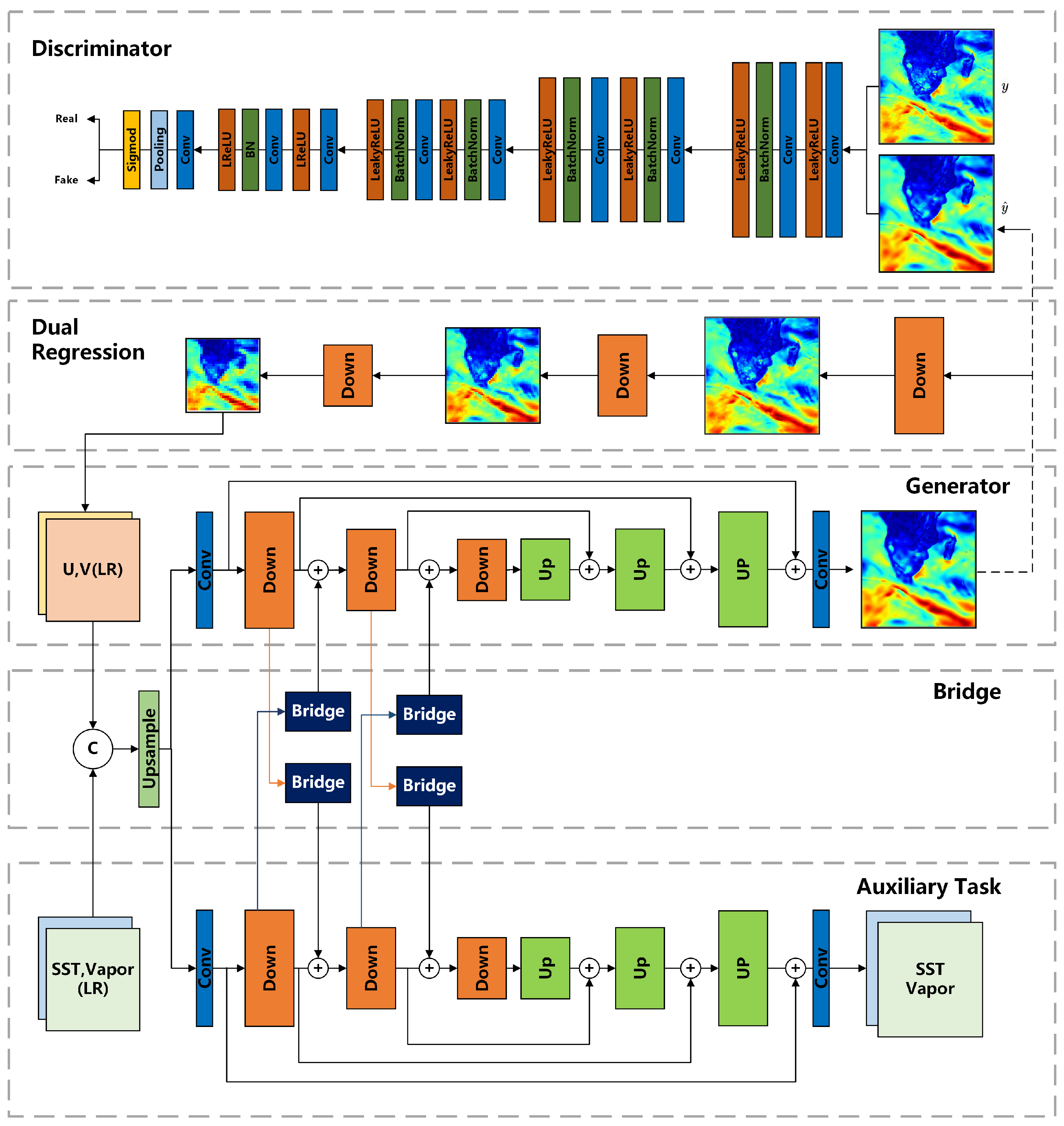
  • A spatial downscaling method for satellite SSW with multi-task learning is proposed. It takes the downscaling of sea surface temperature (SST) and water vapor (WV) as an auxiliary task and incorporates the implicit correlations among variables into downscaling for performance enhancement.
  • A soft-sharing mechanism with bridge modules has been developed to facilitate the sharing of and interaction between tasks.
  • GAN and dual-learning structures have been incorporated into the presented multi-task downscaling network to enhance performance.
  • The results in terms of accuracy compared with buoy observations and reconstruction quality demonstrate the superior performance of the proposed downscaling network.
This paper is structured as follows: Section 2 describes the study area and dataset. Section 3 provides a detailed explanation of the proposed method, encompassing the baseline, auxiliary variables and task, downscaling architecture utilizing soft-sharing multi-task learning, loss function, and training specifications. Section 4 outlines the experimental setup and discusses the results. Concluding remarks are presented in Section 5.

2. Study Area and Dataset
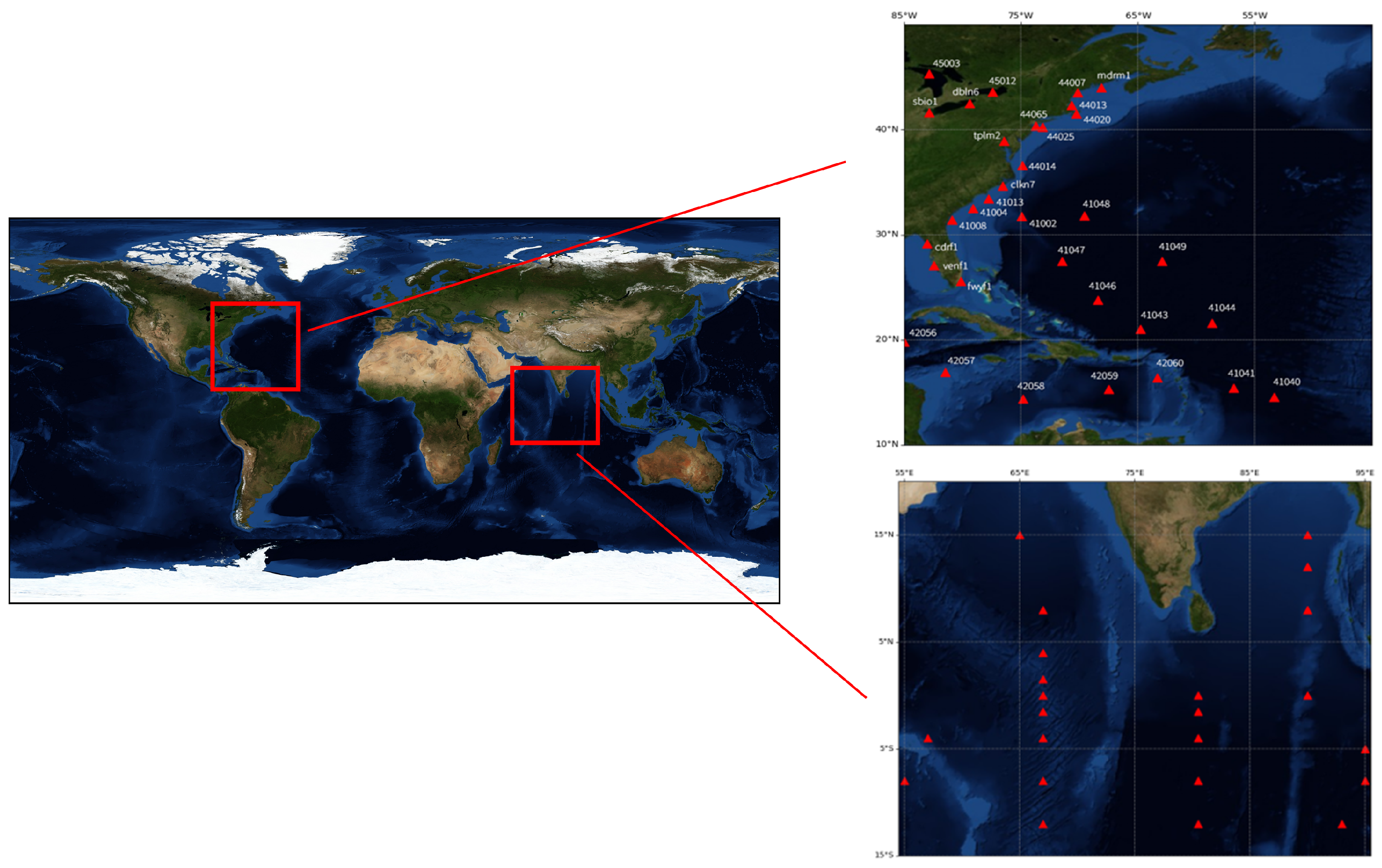
2.1. Study Area

As illustrated in Figure 1, this study focuses on two regions: Region 1, which encompasses the east coast of North America (85°W–45°W longitude and 10°N–50°N latitude), and Region 2, covering the northern Indian Ocean (55°E–95°E longitude and 15°S–20°N latitude). Both Region 1 and Region 2 exhibit abundant climate variability and extreme climate events. In addition, there are sufficient buoy observations in these regions to validate the accuracy of downscaled estimates.

2.2. Dataset

This study leveraged two distinct types of data. The first category comprised data used for model training and evaluation, which included satellite-derived SSW from the radiometer WindSat, along with auxiliary variables, including SST and WV. The paired data for model training of SSW, SST, and WV consisted of the original resolution data (HR) and degraded data (LR), with the LR data being generated from the HR data through bicubic interpolation. A total of three years of satellite data (SSW, SST, and WV) from 2017 to 2019 were collected, including daily products from both ascending and descending orbits. Of these, 80% of the data were randomly assigned as training data, while 20% were designated as test data. The second category consisted of buoy measurements within the study areas, which were used to validate the accuracy of SSW downscaling.

2.2.1. Buoy Data

In Region 1, the buoy SSW measurements are obtained from the National Data Buoy Center (NDBC) of the National Oceanic and Atmospheric Administration (NOAA). For this study, data from 33 NDBC stations were utilized. It is noted that the height of the wind sensors varies across sites. In Region 2, we utilized data from 23 sites of the Research Moored Array for African–Asian–Australian Monsoon Analysis and Prediction (RAMA). These sites are part of the Pacific Marine Environmental Laboratory’s global tropical moored buoy array. RAMA buoys deployed in the Indian Ocean can provide SSW measurements at a height of 4 m. To ensure compatibility with satellite SSW, the wind field data from NDBC and RAMA were calibrated by using the COARE 4.0 algorithm to obtain neutral-equivalent winds at a 10 m reference height [25]. The buoy observations were used to validate the accuracy of downscaled SSW. Specifically, for each buoy observation, the corresponding SSW grid cell is identified based on its spatial location and the matching time period. The accuracy of the SSW is comprehensively evaluated by considering both temporal and spatial consistency.

2.2.2. Satellite Observations

WindSat has been providing accurate SSW data for nearly two decades [46]. This research study utilized the all-weather WindSat v7.0.1 daily SSW dataset from RSS, which has a 0.25° spatial resolution. WindSat, a polarimetric microwave radiometer, resulted from a collaboration between the U.S. Navy and the National Polar-orbiting Operational Environmental Satellite System (NPOESS) Integrated Program Office. The instrument was deployed on 6 January 2003, aboard the Defense Department’s Coriolis satellite. WindSat’s wind vectors have been extensively validated by using buoy measurements and other data products [47].
Previous research indicates that SSW and WV have a relatively close relationship with SST [48]. Moreover, in addition to SSW, the WindSat satellite measures other parameters, including SST and WV, with the same observation times and spatial coverage as SSW. Therefore, considering the relationship with SSW and the data availability, SST and WV are the other two satellite observation data used in this study.

3. Methodology

3.1. Baseline with GAN and Dual Learning

The proposed spatial downscaling method is constructed with a multi-task learning strategy based on a baseline with a GAN and a dual-learning structure, which is proposed in our previous work [25]. The overall architecture is shown in Figure 2.
Generator and discriminator networks form the core components of the GAN architecture [49]. In spatial downscaling, two networks engage in an adversarial process. The generator creates HR SSW while attempting to deceive the discriminator, which in turn strives to distinguish between authentic and generated HR data. This competitive dynamic drives both networks toward equilibrium, ultimately producing increasingly realistic downscaled SSW.
Since the degradation kernel and the HR data are usually unknown in practical scenarios, dual learning has been integrated into the generator of the GAN structure. Dual learning encompasses two key components that form a closed-loop system: the reconstruction of HR SSW fields (primal task) and the estimation of degradation kernels (dual task). These tasks learn simultaneously to achieve optimal performance, where reconstruction functions as the primal task and kernel estimation acts as the regression task. As shown in the left part in Figure 3, y ^ = f ( x ) , x ^ = g ( y ^ ) , x X are LR images, y Y are HR images, and L C o n t e n t and L D u a l are the primal loss and the dual regression loss. Through the closed loop, a downscaling model and a down-sampling model can be obtained. When the downscaling model generates values y ^ closer to y, the values obtained from the down-sampling model, x ^ , will be closer to x. Therefore, the mutual process of two tasks can enhance the downscaling performance of SSW. Furthermore, to constrain the generation of higher SR results, this paper applies the original models of primal and dual tasks in the stage from LR to HR for generating higher SR SSW from HR. As shown in the right part in Figure 3, z = f ( y ) , y = g ( z ) , y Y are HR images, and z Z are SR images. In this extended dual regression paradigm, L D u a l in the right part is the dual regression loss between HR (the original data at 0.25°) and SR.

3.2. Auxiliary Variables and Auxiliary Task

Previous research on SSW has indicated that SSW is correlated with other variables, such as SST and WV [48]. The heat exchange between the ocean and the atmosphere is closely related to the formation of SSW. Ocean waves absorb a considerable part of surface stress and release spray into the atmosphere when they break. The spray evaporates and affects the heat and WV above the waves. The one-dimensional model of the stratified marine surface boundary layer (MSBL) accounts for the impact of waves on the momentum flux and the impact of sea spray on fluxes of heat and moisture [50]. For this model, there are balance equations for momentum, heat, and moisture. Therefore, the aforementioned mechanism provides a rationale for using SST and WV as auxiliary variables in this study. In addition, these two variables are also available in the WindSat data products, with the same observation times and areas.
The existing studies generally stack auxiliary variables with the target as multi-channel inputs. The additional channels and the primal data are fused in the initial stage. It typically applies to the cases where the auxiliary variables are highly correlated with the target variable, and the performance enhancement through data fusion is desired. Therefore, this paper adopts a multi-task learning framework that combines a primary SSW downscaling task with the auxiliary downscaling task for SST and WV. Through simultaneously performing the downscaling of SSW and the auxiliary variables, the relationship among variables is leveraged to improve the downscaling performance of SSW.

3.3. Downscaling Architecture with Soft-Sharing Multi-Task Learning

The spatial downscaling network with soft-sharing multi-task learning has been constructed as shown in Figure 2. The primary task is the spatial downscaling of SSW, and the auxiliary task is the spatial downscaling of SST and WV.
In the downscaling network, the generator adopts an encoder–decoder architecture, and consists of down-sampling modules and up-sampling modules. This design facilitates different downscaling factors by changing the number of modules. For example, for an 8× downscaling network, the number of down-sampling and up-sampling modules is adjusted to l o g 2 8 , accordingly. The down-sampling module consists of a simple 3 × 3 convolutional layer and a LeakyReLU activation function. The convolutional layer includes one convolution with a stride of 2 and another convolution with a stride of 1. The convolution with a stride of 2 reduces the input size by half, thereby achieving the down-sampling effect. The up-sampling module consists of a residual channel attention block (RCAB) [51], convolutional layers, and a PixelShuffle layer. The RCAB module integrates channel attention mechanisms into the residual network. In addition, skip connections are employed to utilize the multi-level information.
In Figure 2, the discriminator consists of convolutional layers, LeakyReLU activation functions, batch standardization layers, adaptive average pooling layers, and sigmoid functions. Among them, the convolutional layer, the LeakyReLU activation function, and the batch standardization layer form four sets of feature extraction layers with gradually decreasing channel numbers and feature sizes. After the last convolutional layer, the number of channels is reduced to 1. Subsequently, an adaptive averaging pooling layer is used to average the features of this channel and obtain a unique value. Finally, this value is passed through the sigmoid function to obtain 0 or 1, where 0 represents false and 1 represents true. The discriminator takes real SSW y and y ^ generated by the generator as inputs and is expected to output 1 when the input is y and output 0 when the input is y ^ .
In addition to the generator and discriminator, this paper introduces the concept of dual learning and incorporates a dual regression structure. The basic idea of dual learning is that two dual tasks can form a closed-loop feedback system, allowing us to obtain feedback from unlabeled data and subsequently utilize this feedback to improve the two machine learning models involved in the dual tasks. The dual regression structure refers to a task network or component that operates in the opposite direction of the original task. In this paper, an additional dual regression structure is introduced to estimate the degradation kernel. It consists of down-sampling blocks, which are the same as that in the generator. The dual regression network down-samples the output of the generator to match the resolution of the generator’s corresponding input, thus forming a dual-learning scheme. In this paper, the additional dual regression structure estimates the degradation kernel. It consists of down-sampling blocks, which are the same as in the generator. The dual regression network down-samples the output of the generator to match the resolution of the generator’s corresponding input, thus forming a dual-learning scheme.
In the multi-task learning setting, the additional auxiliary task performs the downscaling of SST and WV. It adopts the same structure as the basic generator, consisting of several down-sampling blocks and up-sampling blocks with skip connections. For multi-task learning, the way to share parameters is vital for the performance. The hard-parameter-sharing mechanism means that all tasks share several bottom layers after the input and each specific task has a separate branch on top of the shared bottom layers. It requires a high degree of correlation among multiple tasks. For spatial downscaling, the auxiliary input variables have different distributions, and the SR output is strongly correlated with its LR input. Hard sharing can easily result in negative transfer. Unlike the hard-parameter-sharing mechanism, the soft-parameter-sharing mechanism does not directly share the network parameters of the bottom layers. Instead, in the soft-parameter-sharing mechanism, each task has an independent model, but there are constraints between the model parameters. This allows the network to learn its own feature representations for each task, adapting to the differences between tasks. Therefore, this paper uses a soft-sharing multi-task learning network with bridging connections for the spatial downscaling of SSW. The bridge module is composed of stacked RCABs, with the same number of RCABs as in the up-sampling module. The bridge module adjusts the representation of shared features to map the features generated by the auxiliary task to a feature space that is more suitable for the current task. At the same time, the bridge module selectively retains information that is beneficial to the current task through a feature filtering mechanism and suppresses irrelevant features that may introduce interference or cause negative transfer. In this way, the bridge module promotes information sharing between tasks while avoiding the adverse effects on performance caused by feature conflicts.

3.4. Loss Function and Model Training

In this paper, the downscaling of SSW can be expressed by Equation (1), where w represents the downscaling result of SSW, G w represents the generator for SSW downscaling, and φ E s represents the auxiliary task that shares parameters. Similarly, the downscaling of auxiliary variables is shown in Equation (2), where s and G s represent the downscaling result and the generator of auxiliary variable, respectively, and φ E w represents the primary task that shares parameters.
w = G w ( x , φ E s ( x ) ) .
s = G s ( x , φ E w ( x ) ) .
In this context, the total loss of generator L G ( x , y ) includes three items: the content loss L c o n t e n t , the adversarial loss L A d v e r s a l , and the regression loss L d u a l , as shown in Equation (3). The indicator function 1 L R ( x ) is set to 1 when the input includes LR data and 0 when the input includes HR data. The coefficients are used to balance the weights of its components, with λ 1 defaulting to 1 and λ 2 defaulting to 0.1.
L G ( x , y ) = 1 L R ( x ) ( L c o n t e n t ( x , y ) + λ 1 L A d v e r s a r i a l ( x , y w ) + λ 2 L d u a l ( G w ( x , φ E s ( x ) ) , x w ) ) + ( 1 1 L R ( x ) L d u a l ( G w ( x , φ E s ( x ) ) , y w ) ) .
In Equation (4), the content loss of the generator is denoted by L c o n t e n t ( x , y ) , where y w represents the original HR SSW and y s represents the original HR auxiliary data. The weight of the auxiliary task loss is λ 3 . It adjusts the balance of two tasks during model optimization. A larger value of λ 3 corresponds to greater emphasis on the respective branch during optimization. λ 3 is set to 1 at the beginning of model training and can be decreased further when reducing the learning rate.
L c o n t e n t ( x , y ) = | | y w G w ( x , φ E s ( x ) ) | | 2 + λ 3 | | y s G s ( x , φ E w ( x ) ) | | 2 .
L A d v e r s a r i a l represents the adversarial loss and is shown in Equation (5), where D i s is the discriminator. It indicates the discriminator’s assessment of the authenticity of the generated HR SSW y .
L A d v e r s a r i a l ( x , y w ) = l o g D i s ( G w ( x , φ E s ( x ) ) ) .
The dual regression loss L d u a l is shown in Equation (6), where x w is the SSW input by the generator and D u a l is the dual regression model. It calculates the difference between the regression output and the initial input at the same resolution.
L d u a l ( G w ( x , φ E s ( x ) ) , x w ) = | | x w D u a l ( G w ( x , φ w s ( x ) ) ) | | 2 .
In addition, L D i s ( x , y ) measures the discriminator’s loss in distinguishing between the original HR y and the generated data y . It is expected to output 1 for the original data and 0 for the data generated by the generator. The cross entropy loss function is used.
L D i s ( x , y w ) = l o g D i s ( y w ) l o g ( 1 D i s G w ( x , φ E s ( x ) ) ) .
The specific steps of model training are presented in Algorithm 1. There are two different inputs, taking 8× downscaling as an example: the synthetic paired dataset ( x i , y i ) with the original ( 0.25 ) SSW, and auxiliary SST and WV as HR, together with the down-sampled 2 LR; the unpaired data ( y i ) with the 0.25 SSW, SST, and WV as LR. They correspond to two stages in training: supervised learning with paired data ( x i , y i ) and unsupervised dual learning with unpaired data ( y i ) .
Algorithm 1 Model training for spatial downscaling of satellite SSW with auxiliary task
Input SSW, SST, WV ( 0.25 ) as LR: unpaired data ( y i ) ; The corresponding synthetic data as LR ( 2 ) and HR ( 0.25 ) : paired data ( x i , y i )
Ensure: Downscaled SSW results
  1: Initialization models: generator (G), dual regression ( D u a l ) and discriminator ( D i s )
  2: while not convergent do
  3: UnpairedTraining if random(0, 1) < λ U , vice versa
  4: if not Unpaired Training then
  5:  Update D i s by minimizing the objective: Σ L D i s ( x i , y w i )
  6:  Update G by minimizing the objective: Σ L c o n t e n t ( x i , y i ) + λ 1 L A d v e r s a r i a l ( x i , y w i ) + λ 2 L d u a l ( G w ( x i ) , x w i )
  7:  Update D u a l by minimizing the objective: Σ λ 2 L d u a l ( G w ( x i ) , x w i )
  8: else
  9:  Update D u a l by minimizing the objective: Σ λ 2 L d u a l ( G w ( y i ) , y w i )
10: end if
11: end while

4. Experiments and Discussion

4.1. Experimental Setup

The experiments are conducted on a server which is equipped with two Intel Xeon E5-2680v4 CPUs. Each of these CPUs has a base frequency of 2.40 GHz, encompasses 14 cores, and is accompanied by 64 GB of random access memory. Additionally, the server is equipped with an NVIDIA RTX 3090 GPU. The operating system of the server is Ubuntu 20.04.3 LTS, and the software environment includes Python3.8 and PyTorch 1.10.0. During training, the global data are randomly divided into n × n patches, where n is set based on the size of the GPU memory, and the initial learning rate is set to 0.001.
This paper uses two sets of evaluation metrics. Root mean square error (RMSE) and coefficient of determination ( R 2 ) are used to validate the accuracy of the SSW downscaled results. Peak signal-to-noise ratio (PSNR) and structural similarity (SSIM) are employed to evaluate the model’s effectiveness in reconstructing images from LR to HR in the supervised learning stage.

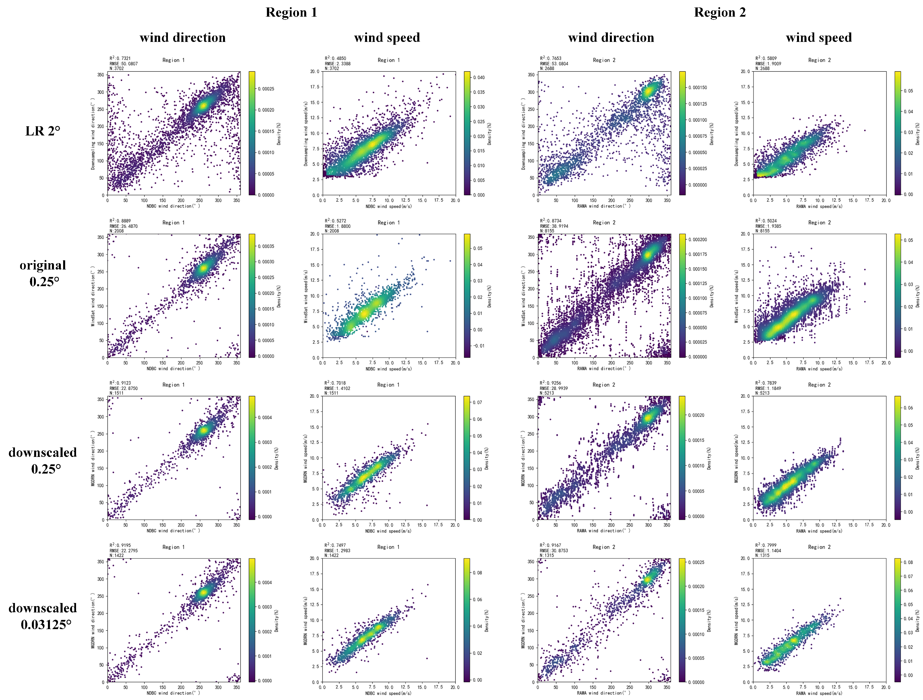
4.2. Validation with Buoy Measurements

This section first trained an 8× downscaling model by using the synthetic paired training dataset (0.25°–2°). The LR degraded data at 2° from the test dataset were input into the model to obtain the downscaled results. The accuracy of the degraded 2° SSW data and the downscaled SSW data were validated with buoy measurements in Region 1 and Region 2, with R M S E and R 2 as the evaluation metrics. The proposed approach attains peak accuracy and significantly outperforms the comparative methods detailed in Section 4.4 once it is downscaled to the original HR of 0.25°. In both Region 1 and Region 2, the RMSE values for wind direction and wind speed are the lowest, at 22.88° and 1.41 m/s, and 28.99° and 1.18 m/s, respectively. The proposed method also achieves the highest R 2 for wind direction and wind speed in both Region 1 and Region 2, at 0.91 and 0.70, and 0.93 and 0.78, respectively.
In practical scenarios, HR ground truths are usually unavailable. To validate the effectiveness of the method proposed when further applied to generate higher-resolution SSW, we subsequently applied the extended dual regression for model training, using the HR data at 0.25° from the test dataset as input to obtain higher-resolution (0.03125°) downscaled SSW on the unpaired dataset. For the downscaling on the unpaired dataset, the proposed method achieves the lowest RMSE for wind direction and wind speed in Regions 1 and 2, with values of 22.28° and 1.30 m/s, and 30.88° and 1.14 m/s, respectively. The proposed method also achieves the highest R 2 values for wind direction and wind speed, with values of 0.92 and 0.75, and 0.92 and 0.80, respectively.
The corresponding scatter plots for accuracy validation with buoy measurements are presented in Figure 4. From left to right, they represent wind direction and wind speed in Region 1 and Region 2. From top to bottom, they show the LR SSW at 2°, the original HR SSW at 0.25°, the downscaling results at 0.25°, and the downscaling results at 0.03125°.

4.3. Impacts of Auxiliary Variables and Task

The downscaling performance of incorporating the auxiliary variables and an auxiliary task has been evaluated. The corresponding impacts on the accuracy and reconstruction quality of downscaled estimations are shown in Table 1 and Table 2. The baseline downscaling method is referred to as SSW. The method of adding auxiliary variables of SST and WV as channels is denoted by SSW + Auxiliary Variable. Multi-Task Downscaling (ours) represents the proposed method, which incorporates an auxiliary task using soft sharing and bridges.
As presented in Table 1, the inclusion of auxiliary variables as extra channel inputs improves the downscaling accuracy. For downscaling on the paired dataset, the RMSE shows a significant reduction compared with the method only using SSW at 0.25°. The RMSEs for wind direction in Region 1 and Region 2 decrease to 23.25° and 30.31°, respectively, while the RMSEs for wind speed in the two study areas decrease to 1.58 m/s and 1.49 m/s, respectively. The R 2 values for both wind speed and wind direction have slightly increased.
The proposed Multi-Task Downscaling method further significantly improves the accuracy of the results. Compared with SSW + Auxiliary Variable, the RMSEs for wind direction in Region 1 and Region 2 have further decreased to 22.88° and 28.99°, corresponding to reductions of 1.59% and 4.35%, respectively. The RMSE values for wind speed have decreased more significantly, dropping to 1.41 m/s and 1.18 m/s, corresponding to reductions of 10.76% and 20.81%, respectively. Additionally, the R 2 values for wind speed have significantly improved, increasing to 0.70 and 0.78 in Region 1 and Region 2, respectively, corresponding to increases of 22.41% and 18.18%.
When extending the proposed method to unpaired datasets, the trends and magnitudes of changes in both RMSE and R 2 are maintained, indicating that incorporating the auxiliary variables and auxiliary task in this study remains effective for obtaining higher-resolution results.
Furthermore, the impact of incorporating the auxiliary variables and auxiliary task on the PSNR and SSIM reconstruction quality metrics has been evaluated by using paired datasets. The corresponding results are presented in Table 2. The proposed Multi-Task Downscaling method further slightly improves the PSNR and SSIM values to 42.62 and 0.986, respectively. This indicates that compared with using only SSW, the downscaled results generated by the proposed method exhibit greater similarity to the original products, with better preservation of details and structures.

4.4. Comparison of Downscaling Methods

The downscaling performance is further evaluated against comparative methods. The results are presented in Table 3, Table 4 and Table 5, with the best results in bold. The representative methods listed include traditional bicubic interpolation, DeepSD, DRN, adversarial DeepSD, GAN-Downscaling, and the proposed Multi-Task Downscaling. As shown in Table 3, the accuracy of the down-sampled data at 2° is low due to their coarse resolution.
In the comparative methods, the bicubic interpolation results at 0.25° improve accuracy compared with the LR input at 2°, but they remain quite lower than the original HR product at 0.25°. The deep learning-based method DeepSD does not show a significant accuracy improvement over bicubic interpolation in the SSW downscaling task. Additionally, its similarity to the original product is lower than that of the interpolation methods. The DRN network, originally designed for single-image super resolution, achieves significant performance improvements in SSW downscaling in terms of accuracy and slightly outperforms bicubic interpolation in PSNR and SSIM. Incorporating a GAN further improves the accuracy when HR ground truth is available in the paired dataset (2°–0.25°). The reconstruction quality metrics also show a slight increase accordingly.
Overall, as shown in Table 1, Table 3 and Table 4, the incorporation of the GAN and dual regression structures, i.e., the SSW method, has achieved superior downscaling performance over the comparative methods. When extended to unpaired datasets, these two structures also show a significant enhancement in downscaling accuracy.
The proposed method achieves the highest accuracy and significantly outperforms the comparative methods. On the paired dataset, the RMSE values for wind direction and wind speed are the lowest in both Region 1 and Region 2, at 22.88° and 1.41 m/s, and 28.99° and 1.18 m/s, respectively. Compared with the best results of the comparative methods (GAN-Downscaling), this represents further decreases of 1.54° and 0.21 m/s in Region 1 and 5.08° and 0.39 m/s in Region 2, corresponding to decreases of 6.31%, 12.96%, 4.91%, and 24.84%, respectively. The proposed method achieves the highest R 2 for wind direction and wind speed in both Region 1 and Region 2, at 0.91 and 0.70, and 0.93 and 0.78, respectively. The improvement in R 2 for wind speed is particularly notable. In Table 4, the proposed method achieves a more significant performance improvement on high-resolution unpaired datasets compared with low-resolution paired datasets, when compared with other methods. In Table 5, the reconstruction quality of the proposed method in terms of PSNR and SSIM significantly outperforms that of the comparative methods.

4.5. Computational Efficiency

In practical applications, in addition to focusing on the accuracy of downscaling and the quality of reconstruction, computational efficiency is also an important indicator for evaluating the practicality of a method. Especially in scenarios where large-scale datasets need to be processed, computational efficiency becomes even more important. In order to comprehensively evaluate the efficiency performance of the model, this paper uses the commonly used floating-point operations (FLOPs) and model parameter indicators for analysis. We list the model parameters and FLOPs in detail in Table 6. It should be noted that in the model inference stage (i.e., the downscaling process), only the generator model is used for calculation. Therefore, for GAN-based methods, their inference efficiency indicators are consistent with the corresponding generator model. In addition, for fair comparison, the comparison methods uniformly use fixed-size input tensors (3, 40, 40) to measure FLOPs, while Multi-Task Downscaling requires additional auxiliary data, so its FLOPs is measured based on the input size (4, 40, 40).
Since the Multi-Task Downscaling method adopts a multi-task dual-generation branch model design, its parameter volume reaches 22,800,202, and the FLOPs is 154.25 G, which are significantly higher compared with other comparison methods. This model design improves the expressiveness and reconstruction quality of the downscaling method by introducing additional task branches and richer input features. Although this improvement brings an increase in computational cost, its parameter volume and FLOPs are still within an acceptable range in practical applications and can meet the processing requirements of larger-scale datasets.

4.6. Model Transferability

Although the method of this study was only verified in two specific regions, our training process was not limited to these areas. The selection of these regions was primarily based on their representativeness in related studies [52,53,54] and the availability of high-quality buoy data for validation. However, in order to more comprehensively evaluate the robustness and universality of the method, it is necessary to further explore its applicability in regions with different climate and ocean conditions.
In terms of climate conditions, different sea areas may have significant wind field variation characteristics, such as strong convection and typhoon activities in tropical areas, strong wind effects in high-latitude areas, etc. These special climate phenomena may affect the prediction accuracy of SSW. In terms of ocean conditions, the distribution characteristics of auxiliary variables such as SST and WV may vary from region to region, thereby affecting the generalization performance of the method. Therefore, in future studies, applying the method to a variety of typical regions (such as tropical seas, high-latitude seas, etc.) for testing will help to more comprehensively evaluate its applicability.
In addition, in order to enhance the migration ability of the method, domain adaptation technology or methods based on transfer learning can be introduced to better handle the distribution differences between different regions. At the same time, by increasing the diversity of data sources, such as combining satellite remote sensing data with measured data, the generalization and stability of the method can be further improved.

4.7. Robustness Evaluation Under Noisy Low-Quality Data

To evaluate the robustness of the proposed model under real-world data conditions, we added white noise with an amplitude range of 1 m/s to the down-sampled 2° data. The bicubic interpolation method used to down-sample the data from 0.25° to 2° resolution reduces high-frequency noise, which causes the data to be overly smoothed, thus outperforming the actual situation in the experiment. Adding noise is necessary to better simulate real-world conditions. In addition, adding noise to the down-sampled 2° data can also explore the impact of the degradation of input data quality on model performance.
From the experimental results in Table 7, the performance of all methods has different degrees of degradation after adding noise, which shows that the quality of input data has a significant impact on model performance. However, the proposed method still performs best in all experiments, showing its superiority in dealing with noisy and low-quality input data. This may be because the introduction of auxiliary variables and tasks enhances the model’s adaptability to input noise.

4.8. Uncertainty Analysis

Uncertainty analysis is a crucial aspect in evaluating the reliability and robustness of predictive models. In this study, an ensemble modeling approach was employed for uncertainty analysis. The proposed model was randomly initialized and trained five times to create five independent models. These models were then used to generate predictions for each sample, resulting in five output values per sample. To quantify uncertainty, standard deviation was used as the evaluation metric, as it effectively captures the dispersion of predictions around their mean. A lower standard deviation indicates higher model stability and reliability, while a higher standard deviation suggests greater variability and potential inconsistency in the predictions. The experimental results show that the average standard deviation of the proposed method is 0.478 m/s for wind speed and 8.72° for wind direction, highlighting its strong robustness and reliability.

5. Conclusions

In this paper, a novel spatial downscaling method for satellite SSW with soft-sharing multi-task learning has been put forward. Unlike the majority of existing spatial downscaling studies based on deep learning that typically rely on single-image super resolution, this paper attempts to further capture the correlation among variables. Considering the close correlation between SSW and other variables revealed by existing physical processes and the data availability within the same spatial and temporal ranges, SST and WV are included as auxiliary variables. A multi-task learning network with GAN and dual regression structures for spatial downscaling has been developed. Specifically, the soft-parameter-sharing mechanism with bridge modules has been leveraged for the interaction of complementary features between tasks. Comprehensive experiments have been conducted with WindSat SSW products at 0.25° from RSS. The outcomes demonstrate that the proposed method has attained remarkable downscaling performance, especially when considering accuracy in relation to buoy measurements and the quality of reconstruction. Moreover, the proposed method surpasses the comparative methods when applied to synthetic paired datasets (2°–0.25°) and can also be effectively extended to unpaired datasets (0.25° as LR) to generate higher-resolution estimates. The proposed method demonstrates the capability to generate high-resolution satellite SSW estimations with high accuracy and reconstruction quality. Furthermore, this method can serve as a reference for downscaling other meteorological variables. Currently, preliminary uncertainty quantification has been performed for the proposed method. Future research will focus on further refining and expanding the uncertainty quantification process. This will involve a comprehensive analysis of the uncertainties of the proposed method and comparison approaches.

Author Contributions

Y.Y.: Writing—review and editing; Writing—original draft. J.L.: Writing—review and editing; Writing—original draft; Investigation; Formal analysis. Y.S.: Writing—review and editing; Formal analysis. K.R.: Writing—review and editing. K.D. (Kefeng Deng): Writing—review and editing; Methodology. K.D. (Ke Deng): Writing—review and editing. All authors have read and agreed to the published version of the manuscript.

Funding

This work was funded by Science and Technology Innovation Program of Hunan Province (2022RC3070). It also received support from National Natural Science Foundation of China under grant 41901376 and Key Laboratory of Smart Earth No. KF2023YB03-09.

Institutional Review Board Statement

Not applicable.

Informed Consent Statement

Not applicable.

Data Availability Statement

Data will be available upon request from the corresponding author.

Acknowledgments

The authors would like to thank the Remote Sensing Systems for freely providing the sea surface wind, sea surface temperature, and water vapor data. They would also like to thank the National Data Buoy Center of the National Oceanic and Atmospheric Administration and Research Moored Array for African–Asian–Australian Monsoon Analysis and Prediction for freely providing the buoy data.

Conflicts of Interest

Author Ke Deng was employed by the company Fiberhome Telecommunication Technologies Co., Ltd. The remaining authors declare that the research was conducted in the absence of any commercial or financial relationships that could be construed as a potential conflict of interest.

References

  1. Liu, G.; Yang, X.; Li, X.; Zhang, B.; Pichel, W.; Li, Z.; Zhou, X. A Systematic Comparison of the Effect of Polarization Ratio Models on Sea Surface Wind Retrieval From C-Band Synthetic Aperture Radar. IEEE J. Sel. Top. Appl. Earth Obs. Remote Sens. 2013, 6, 1100–1108. [Google Scholar] [CrossRef]
  2. Zhang, K.; Xu, X.; Han, B.; Mansaray, L.R.; Guo, Q.; Huang, J. The Influence of Different Spatial Resolutions on the Retrieval Accuracy of Sea Surface Wind Speed with C-2PO Models Using Full Polarization C-Band SAR. IEEE Trans. Geosci. Remote Sens. 2017, 55, 5015–5025. [Google Scholar] [CrossRef]
  3. Hu, T.; Li, Y.; Li, Y.; Wu, Y.; Zhang, D. Retrieval of Sea Surface Wind Fields Using Multi-Source Remote Sensing Data. Remote Sens. 2020, 12, 1482. [Google Scholar] [CrossRef]
  4. Ren, F.; Li, Y.; Zheng, Z.; Yan, H.; Du, Q. Online emergency mapping based on disaster scenario and data integration. Int. J. Image Data Fusion 2021, 12, 282–300. [Google Scholar] [CrossRef]
  5. Shuai, P.; Chen, X.Y.; Mital, U.; Coon, E.T.; Dwivedi, D. The effects of spatial and temporal resolution of gridded meteorological forcing on watershed hydrological responses. Hydrol. Earth Syst. Sci. 2022, 26, 2245–2276. [Google Scholar] [CrossRef]
  6. De Caceres, M.; Martin-StPaul, N.; Turco, M.; Cabon, A.; Granda, V. Estimating daily meteorological data and downscaling climate models over landscapes. Environ. Model. Softw. 2018, 108, 186–196. [Google Scholar] [CrossRef]
  7. Tapiador, F.J.; Navarro, A.; Moreno, R.; Sanchez, J.L.; Garcia-Ortega, E. Regional climate models: 30 years of dynamical downscaling. Atmos. Res. 2020, 235, 104785. [Google Scholar] [CrossRef]
  8. Xu, Z.F.; Han, Y.; Yang, Z.L. Dynamical downscaling of regional climate: A review of methods and limitations. Sci. China Earth Sci. 2019, 62, 365–375. [Google Scholar] [CrossRef]
  9. Wang, S.M.; Luo, Y.M.; Li, X.; Yang, K.X.; Liu, Q.; Luo, X.B.; Li, X.H. Downscaling land surface temperature based on non-linear geographically weighted regressive model over urban areas. Remote Sens. 2021, 13, 1580. [Google Scholar] [CrossRef]
  10. Tang, J.P.; Niu, X.R.; Wang, S.Y.; Gao, H.X.; Wang, X.Y.; Wu, J. Statistical downscaling and dynamical downscaling of regional climate in China: Present climate evaluations and future climate projections. J. Geophys. Res. Atmos. 2016, 121, 2110–2129. [Google Scholar] [CrossRef]
  11. Sachindra, D.A.; Ahmed, K.; Rashid, M.M.; Shahid, S.; Perera, B.J.C. Statistical downscaling of precipitation using machine learning techniques. Atmos. Res. 2018, 212, 240–258. [Google Scholar] [CrossRef]
  12. Camus, P.; Menéndez, M.; Méndez, F.J.; Izaguirre, C.; Espejo, A.; Cánovas, V.; Pérez, J.; Rueda, A.; Losada, I.J.; Medina, R. A weather-type statistical downscaling framework for ocean wave climate. J. Geophys. Res. Oceans 2014, 119, 7389–7405. [Google Scholar] [CrossRef]
  13. Jia, S.; Zhu, W.; Lu, A.; Yan, T. A statistical spatial downscaling algorithm of TRMM precipitation based on NDVI and DEM in the Qaidam Basin of China. Remote Sens. Environ. 2011, 115, 3069–3079. [Google Scholar] [CrossRef]
  14. Skourkeas, A.; Kolyva-Machera, F.; Maheras, P. Improved statistical downscaling models based on canonical correlation analysis, for generating temperature scenarios over Greece. Environ. Ecol. Stat. 2013, 20, 445–465. [Google Scholar] [CrossRef]
  15. Martinez, Y.; Yu, W.; Lin, H. A New Statistical-Dynamical Downscaling Procedure Based on EOF Analysis for Regional Time Series Generation. J. Appl. Meteorol. Climatol. 2013, 52, 935–952. [Google Scholar] [CrossRef]
  16. Yan, X.; Chen, H.; Tian, B.; Sheng, S.; Wang, J.; Kim, J.S. A Downscaling-Merging Scheme for Improving Daily Spatial Precipitation Estimates Based on Random Forest and Cokriging. Remote Sens. 2021, 13, 2040. [Google Scholar] [CrossRef]
  17. Sa’adi, Z.; Shahid, S.; Pour, S.H.; Ahmed, K.; Chung, E.S.; Yaseen, Z.M. Multi-variable model output statistics downscaling for the projection of spatio-temporal changes in rainfall of Borneo Island. J. Hydro-Environ. Res. 2020, 31, 62–75. [Google Scholar] [CrossRef]
  18. Martin, T.C.M.; Rocha, H.R.; Perez, G.M.P. Fine scale surface climate in complex terrain using machine learning. Int. J. Climatol. 2021, 41, 233–250. [Google Scholar] [CrossRef]
  19. Yang, W.M.; Zhang, X.C.; Tian, Y.P.; Wang, W.; Xue, J.H.; Liao, Q.M. Deep learning for single image super-resolution: A brief review. IEEE Trans. Multimed. 2019, 21, 3106–3121. [Google Scholar] [CrossRef]
  20. Hohlein, K.; Kern, M.; Hewson, T.; Westermann, R. A comparative study of convolutional neural network models for wind field downscaling. Meteorol. Appl. 2020, 27, e1961. [Google Scholar] [CrossRef]
  21. Dujardin, J.; Lehning, M. Wind-Topo: Downscaling near-surface wind fields to high-resolution topography in highly complex terrain with deep learning. Q. J. R. Meteorol. Soc. 2022, 148, 1368–1388. [Google Scholar] [CrossRef]
  22. Yu, T.; Yang, R.; Huang, Y.; Gao, J.; Kuang, Q. Terrain-guided flatten memory network for deep spatial wind downscaling. IEEE J. Sel. Top. Appl. Earth Obs. Remote Sens. 2022, 15, 9468–9481. [Google Scholar] [CrossRef]
  23. Zhang, S.Y.; Li, X.C. Future projections of offshore wind energy resources in China using CMIP6 simulations and a deep learning-based downscaling method. Energy 2021, 217, 119321. [Google Scholar] [CrossRef]
  24. Stengel, K.; Glaws, A.; Hettinger, D.; King, R.N. Adversarial super-resolution of climatological wind and solar data. Proc. Natl. Acad. Sci. USA 2020, 117, 16805–16815. [Google Scholar] [CrossRef]
  25. Liu, J.; Sun, Y.J.; Ren, K.J.; Zhao, Y.L.; Deng, K.F.; Wang, L.Z. A spatial downscaling approach for WindSat satellite sea surface wind based on generative adversarial networks and dual learning scheme. Remote Sens. 2022, 14, 769. [Google Scholar] [CrossRef]
  26. Gerges, F.; Boufadel, M.C.; Bou-Zeid, E.; Nassif, H.; Wang, J.T.L. A Novel Bayesian Deep Learning Approach to the Downscaling of Wind Speed with Uncertainty Quantification. In Proceedings of the Advances in Knowledge Discovery and Data Mining, PAKDD 2022, PT III, Chengdu, China, 16–19 May 2022; Gama, J., Li, T., Yu, Y., Chen, E., Zheng, Y., Teng, F., Eds.; Lecture Notes in Artificial Intelligence. Springer: Cham, Switzerland, 2022; Volume 13282, pp. 55–66. [Google Scholar] [CrossRef]
  27. Doury, A.; Somot, S.; Gadat, S.; Ribes, A.; Corre, L. Regional climate model emulator based on deep learning: Concept and first evaluation of a novel hybrid downscaling approach. Clim. Dyn. 2023, 60, 1751–1779. [Google Scholar] [CrossRef]
  28. Rampal, N.; Gibson, P.B.; Sood, A.; Stuart, S.; Fauchereau, N.C.; Brandolino, C.; Noll, B.; Meyers, T. High-resolution downscaling with interpretable deep learning: Rainfall extremes over New Zealand. Weather Clim. Extrem. 2022, 38, 100525. [Google Scholar] [CrossRef]
  29. Sun, Y.; Deng, K.; Ren, K.; Liu, J.; Deng, C.; Jin, Y. Deep learning in statistical downscaling for deriving high spatial resolution gridded meteorological data: A systematic review. ISPRS J. Photogramm. Remote Sens. 2024, 208, 14–38. [Google Scholar] [CrossRef]
  30. Wang, F.; Tian, D.; Lowe, L.; Kalin, L.; Lehrter, J. Deep learning for daily precipitation and temperature downscaling. Water Resour. Res. 2021, 57, e2020WR029308. [Google Scholar] [CrossRef]
  31. Vandal, T.; Kodra, E.; Ganguly, S.; Michaelis, A.; Nemani, R.; Ganguly, A.R. DeepSD: Generating high resolution climate change projections through single image super-resolution. In Proceedings of the 23rd ACM SIGKDD International Conference on Knowledge Discovery and Data Mining (KDD ’17), Halifax, NS, Canada, 13–17 August 2017; Association for Computing Machinery: New York, NY, USA, 2017; pp. 1663–1672. [Google Scholar] [CrossRef]
  32. Sha, Y.K.; Gagne, D.J.; West, G.; Stull, R. Deep-learning-based gridded downscaling of surface meteorological variables in complex terrain. Part II: Daily precipitation. J. Appl. Meteorol. Clim. 2020, 59, 2075–2092. [Google Scholar] [CrossRef]
  33. Tie, R.; Shi, C.; Wan, G.; Hu, X.; Kang, L.; Ge, L. CLDASSD: Reconstructing fine textures of the temperature field using super-resolution technology. Adv. Atmos. Sci. 2022, 39, 117–130. [Google Scholar] [CrossRef]
  34. Sha, Y.K.; Gagne, D.J.; West, G.; Stull, R. Deep-learning-based gridded downscaling of surface meteorological variables in complex terrain. Part I: Daily maximum and minimum 2-m temperature. J. Appl. Meteorol. Clim. 2020, 59, 2057–2073. [Google Scholar] [CrossRef]
  35. Harris, L.; McRae, A.T.T.; Chantry, M.; Dueben, P.D.; Palmer, T.N. A generative deep learning approach to stochastic downscaling of precipitation forecasts. J. Adv. Model. Earth Syst. 2022, 14, e2022MS003120. [Google Scholar] [CrossRef] [PubMed]
  36. Hewson, T.D.; Pillosu, F.M. A low-cost post-processing technique improves weather forecasts around the world. Commun. Earth Environ. 2021, 2, 132. [Google Scholar] [CrossRef]
  37. Bano-Medina, J.; Manzanas, R.; Gutierrez, J.M. Configuration and intercomparison of deep learning neural models for statistical downscaling. Geosci. Model Dev. 2020, 13, 2109–2124. [Google Scholar] [CrossRef]
  38. Bano-Medina, J.; Manzanas, R.; Manuel Gutierrez, J. On the suitability of deep convolutional neural networks for continental-wide downscaling of climate change projections. Clim. Dyn. 2021, 57, 2941–2951. [Google Scholar] [CrossRef]
  39. Sun, L.; Lan, Y. Statistical downscaling of daily temperature and precipitation over China using deep learning neural models: Localization and comparison with other methods. Int. J. Climatol. 2021, 41, 1128–1147. [Google Scholar] [CrossRef]
  40. Jin, W.; Luo, Y.; Wu, T.; Huang, X.; Xue, W.; Yu, C. Deep learning for seasonal precipitation prediction over China. J. Meteorol. Res. 2022, 36, 271–281. [Google Scholar] [CrossRef]
  41. Pan, B.; Hsu, K.; AghaKouchak, A.; Sorooshian, S. Improving precipitation estimation using convolutional neural network. Water Resour. Res. 2019, 55, 2301–2321. [Google Scholar] [CrossRef]
  42. Adewoyin, R.A.; Dueben, P.; Watson, P.; He, Y.L.; Dutta, R. TRU-NET: A deep learning approach to high resolution prediction of rainfall. Mach. Learn. 2021, 110, 2035–2062. [Google Scholar] [CrossRef]
  43. Jin, X.; Xu, J.; Tasaka, K.; Chen, Z. Multi-task Learning-based All-in-one Collaboration Framework for Degraded Image Super-resolution. ACM Trans. Multimed. Comput. Commun. Appl. 2021, 17, 21. [Google Scholar] [CrossRef]
  44. Zhang, Y.; Yang, Q. A Survey on Multi-Task Learning. IEEE Trans. Knowl. Data Eng. 2022, 34, 5586–5609. [Google Scholar] [CrossRef]
  45. Thung, K.H.; Wee, C.Y. A brief review on multi-task learning. Multimed. Tools Appl. 2018, 77, 29705–29725. [Google Scholar] [CrossRef]
  46. Hilburn, K.A.; Meissner, T.; Wentz, F.J.; Brown, S.T. Ocean Vector Winds From WindSat Two-Look Polarimetric Radiances. IEEE Trans. Geosci. Remote Sens. 2016, 54, 918–931. [Google Scholar] [CrossRef]
  47. Zheng, M.; Li, X.M.; Sha, J. Comparison of sea surface wind field measured by HY-2A scatterometer and WindSat in global oceans. J. Oceanol. Limnol. 2019, 37, 38–46. [Google Scholar] [CrossRef]
  48. Jacobs, R.A.; Jordan, M.I.; Nowlan, S.J.; Hinton, G.E. Adaptive mixtures of local experts. Neural Comput. 1991, 3, 79–87. [Google Scholar] [CrossRef]
  49. Creswell, A.; White, T.; Dumoulin, V.; Arulkumaran, K.; Sengupta, B.; Bharath, A.A. Generative adversarial networks: An overview. IEEE Signal Process Mag. 2018, 35, 53–65. [Google Scholar] [CrossRef]
  50. Makin, V. Air-sea exchange of heat in the presence of wind waves and spray. J. Geophys. Res. Oceans 1998, 103, 1137–1152. [Google Scholar] [CrossRef]
  51. Zhang, Y.; Li, K.; Li, K.; Wang, L.; Zhong, B.; Fu, Y. Image Super-Resolution Using Very Deep Residual Channel Attention Networks. In Proceedings of the Computer Vision—ECCV 2018, Munich, Germany, 8–14 September 2018; Ferrari, V., Hebert, M., Sminchisescu, C., Weiss, Y., Eds.; Springer: Cham, Switzerland, 2018; pp. 294–310. [Google Scholar]
  52. Yao, Z.; Xue, Z.; He, R.; Bao, X.; Song, J. Statistical downscaling of IPCC sea surface wind and wind energy predictions for US east coastal ocean, Gulf of Mexico and Caribbean Sea. J. Ocean Univ. China 2016, 15, 577–582. [Google Scholar] [CrossRef]
  53. Fernández-Alvarez, J.C.; Costoya, X.; Pérez-Alarcón, A.; Rahimi, S.; Nieto, R.; Gimeno, L. Dynamic downscaling of wind speed over the North Atlantic Ocean using CMIP6 projections: Implications for offshore wind power density. Energy Rep. 2023, 9, 873–885. [Google Scholar] [CrossRef]
  54. Kolukula, S.S.; Murty, P.; Baduru, B.; Sharath, D.; PA, F. Downscaling of wind fields on the east coast of India using deep convolutional neural networks and their applications in storm surge computations. J. Water Clim. Chang. 2024, 15, 1612–1628. [Google Scholar] [CrossRef]
Figure 1. The study areas of the spatial downscaling of SSW: Region 1, the east coast of North America, and Region 2, the northern Indian Ocean. The red triangles represent the buoy stations.
Remotesensing 17 00587 g001
Figure 2. The network architecture of the proposed spatial downscaling method.
Remotesensing 17 00587 g002
Figure 3. The extended dual regression downscaling scheme with the primal task and the dual task. The left shows the original mapping between LR and HR, and the right shows the extended mapping between HR and SR [25]. The colors represent wind speed values.
Remotesensing 17 00587 g003
Figure 4. The scatter plots for accuracy validation against buoy measurements in study areas.
Remotesensing 17 00587 g004
Table 1. Impacts of auxiliary variable and auxiliary task on accuracy of downscaled estimations. The bold indicates the optimal metric among the comparison methods.
TypeResolutionMethodComponentRegion 1Region 2
RMSER2RMSER2
LRBicubic down-sample 8×Direction50.080.7353.080.77
Speed2.340.491.900.58
Downscaling HR0.25°SSWDirection24.870.9035.020.90
Speed1.690.621.680.63
SSW + Auxiliary VariableDirection23.250.9130.310.92
Speed1.580.621.490.66
Multi-Task Downscaling (ours)Direction22.880.9128.990.93
Speed1.410.701.180.78
Downscaling SR0.03125°SSWDirection25.190.9037.630.88
Speed1.780.581.750.60
SSW + Auxiliary VariableDirection23.490.9131.450.91
Speed1.400.711.400.70
Multi-Task Downscaling (ours)Direction22.280.9230.880.92
Speed1.300.751.140.80
Table 2. Impacts of auxiliary variable and auxiliary task on reconstruction quality of downscaled estimations. The bold indicates the optimal metric among the comparison methods.
MethodPSNRSSIM
SSW40.160.982
SSW + Auxiliary Variable40.280.971
Multi-Task Downscaling (ours)42.620.986
Table 3. The accuracy validation comparison of downscaled SSW on the paired dataset (2°–0.25°). The bold indicates the optimal metric among the comparison methods.
TypeResolutionMethodComponentRegion 1Region 2
RMSER2RMSER2
LRBicubic down-sample 8×Direction50.080.7353.080.77
Speed2.340.491.900.58
Downscaling HR0.25°Bicubic interpolationDirection34.530.8144.140.83
Speed1.900.521.850.55
DeepSDDirection34.380.8144.280.83
Speed2.120.401.960.49
Adversarial DeepSDDirection28.720.8738.320.88
Speed2.080.421.870.54
DRNDirection26.110.8936.480.89
Speed1.910.511.660.63
GAN-DownscalingDirection24.420.9134.070.90
Speed1.620.651.570.67
Multi-Task Downscaling (ours)Direction22.880.9128.990.93
Speed1.410.701.180.78
Table 4. The accuracy validation of downscaled SSW on the unpaired dataset (0.25°–0.03125°). The bold indicates the optimal metric among the comparison methods.
TypeResolutionMethodComponentRegion 1Region 2
RMSER2RMSER2
Original HR0.25°Original HRDirection26.490.8938.920.87
Speed1.880.531.940.50
Downscaling SR0.03125°Bicubic interpolationDirection26.070.9038.710.88
Speed1.820.571.960.49
DeepSDDirection29.440.8742.480.85
Speed2.210.362.160.38
Adversarial DeepSDDirection32.280.8445.260.83
Speed2.160.392.240.34
DRNDirection31.010.8544.240.84
Speed2.090.432.160.38
GAN-DownscalingDirection30.800.8643.960.84
Speed1.820.562.020.46
Multi-Task Downscaling (ours)Direction22.280.9230.880.92
Speed1.300.751.140.80
Table 5. The reconstruction quality of SSW in the supervised learning stage. The bold indicates the optimal metric among the comparison methods.
MethodPSNRSSIM
Bicubic38.340.973
DeepSD36.750.951
Adversarial DeepSD36.890.958
DRN39.430.977
GAN-Downscaling39.960.980
Multi-Task Downscaling (ours)42.620.986
Table 6. The parameters and FLOPs of the model during model inference.
ResolutionMethodParametersFLOPs
8× downscalingBicubic interpolation0102.4 K
DeepSD207,82516.4 G
Adversarial DeepSD207,82516.4 G
DRN10,000,77263.57 G
GAN-Downscaling10,000,77263.57 G
Multi-Task Downscaling (ours)22,800,202154.25 G
Table 7. Accuracy verification comparison of downscaled SSW on noisy input data (2°–0.25°). The bold indicates the optimal metric among the comparison methods.
TypeResolutionMethodComponentRegion 1Region 2
RMSER2RMSER2
LRBicubic down-sample 8×Direction50.080.7353.080.77
Speed2.530.402.160.46
Downscaling HR0.25°Bicubic interpolationDirection34.410.8144.370.83
Speed2.110.411.990.47
DeepSDDirection34.540.8144.330.83
Speed2.180.362.000.47
Adversarial DeepSDDirection28.850.8738.790.87
Speed2.170.371.940.50
DRNDirection26.280.8937.250.88
Speed2.140.391.840.55
GAN-DownscalingDirection26.650.8836.140.90
Speed1.910.511.820.60
Multi-Task Downscaling (ours)Direction23.020.9128.740.93
Speed1.420.701.180.79
Disclaimer/Publisher’s Note: The statements, opinions and data contained in all publications are solely those of the individual author(s) and contributor(s) and not of MDPI and/or the editor(s). MDPI and/or the editor(s) disclaim responsibility for any injury to people or property resulting from any ideas, methods, instructions or products referred to in the content.

