Article

Exploring the Long-Term Relationship Between Thermospheric ∑O/N2 and Solar EUV Flux

1
Institute for Frontiers in Astronomy and Astrophysics, Beijing Normal University, Beijing 102206, China
2
School of Physics and Astronomy, Beijing Normal University, Beijing 100875, China
3
Macau Institute of Space Technology and Application, Macau University of Science and Technology, Macau, China
*
Author to whom correspondence should be addressed.
Remote Sens. 2025, 17(4), 574; https://doi.org/10.3390/rs17040574
Submission received: 7 January 2025 / Revised: 29 January 2025 / Accepted: 3 February 2025 / Published: 8 February 2025

Abstract

:
Column O/N2 ratio (∑O/N2), a physical quantity representing thermospheric disturbances, is influenced by solar extreme ultraviolet radiation flux (QEUV) changes. Investigating the correlation between these two factors is essential for understanding the evolution of the thermosphere. This study examines the correlation and periodic variations of ∑O/N2 and QEUV across different phases of solar activity, using data from the Global Ultraviolet Imager (GUVI) spanning from 2002 to 2022. A correlation analysis reveals a positive relationship between ∑O/N2 and QEUV. The function fitting results show that the magnitude of changes in ∑O/N2 due to QEUV variations is approximately 30% of the mean ∑O/N2. A wavelet analysis reveals their coherence in periodic components of 27-day, annual, and 11-year periods. These results are significant for studying the Sun–Earth coupling mechanism and understanding the impact of space weather on the thermosphere.

Graphical Abstract

1. Introduction

Column O/N2 ratio (∑O/N2) was first proposed by Strickland [1]. This physical quantity can effectively reflect the changes in neutral components and disturbances in the thermosphere, so it has received widespread attention in thermosphere-related studies, with many observational and modeling studies conducted on this quantity [2,3]. ∑O/N2 has an important connection with electron density in the ionospheric F-region and total electron density. Studying ∑O/N2 is significant for monitoring changes in ionospheric electron density [4]. ∑O/N2 is also an important indicator of thermospheric disturbances caused by geomagnetic activity [5]. Therefore, studying the variation in ∑O/N2 is of great significance for understanding thermospheric processes and evolution.
∑O/N2 is influenced by various factors, such as geomagnetic storms [5,6], particle and Joule heating [7], inter-hemispheric transport [8], seasonal effects [9,10], atmospheric waves [11], and the energy and momentum input from solar radiation [12]. Solar radiation plays an important role in the long-term variation in ∑O/N2, with solar extreme ultraviolet (EUV) radiation having a significant impact on ∑O/N2 changes.
EUV radiation, consisting of high-energy photons with wavelengths between 10 and 121 nm, is intensely absorbed by molecular oxygen and molecular nitrogen in the thermosphere. This absorption causes atmospheric heating, the photodissociation of molecules, and ionization, which highlights how EUV radiation can strongly influence the temperature and composition distribution in the thermosphere [13]. Therefore, investigating the relationship between ∑O/N2 and EUV flux (QEUV) is essential for gaining a deeper understanding of the effects of solar activity on the thermosphere and the underlying physical mechanisms.
Thiemann’s study indicates that variations in QEUV affect thermospheric O/N2, with a positive correlation between them [14]. Strickland et al. report a strong correspondence between ∑O/N2 and QEUV, suggesting that ∑O/N2 can be used to determine QEUV [1,15]. Meier’s study derives QEUV irradiance from ∑O/N2 and LBH/135.6 nm data from GUVI measurements [16]. Zhang’s study identifies a strong positive correlation between ∑O/N2 and QEUV and indicates an exponential fitting relationship between them through the analysis of TIMED/GUVI data from 2002 to 2007 [17]. Several perspectives exist regarding the physical mechanisms by which QEUV affects ∑O/N2. QEUV influences thermospheric photochemical processes, leading to changes in neutral components such as O and N2 [18]. Solar radiation heating influences atmospheric circulation and wave effects (e.g., the “thermospheric spoon” effect due to uneven heating [19]), which leads to the transport of components such as O and N2 [20,21]. Some argue that QEUV variations could lead to changes in the reference altitude of ∑O/N2 [17], but this perspective has been considered contentious as it overlooks the connection between remote sensing spectra and ∑O/N2 [22,23].
One study analyzed the variations between the two during the declining phase of the 23rd solar cycle [17], but the correlation between ∑O/N2 and QEUV over longer timescales (spanning multiple solar cycles) remains unclear, and potential differences in their relationship across distinct solar activity phases warrant further study. Investigating the periodicity of ∑O/N2 and QEUV is crucial for understanding their relationship, and exploring the coherence between their periodic components is important. Using remote sensing data from the Global Ultraviolet Imager (GUVI) spanning from 2002 to 2022, we aim to investigate the long-term variations and correlations between ∑O/N2 and QEUV, and contrast their relationship across different phases of solar activity. We also analyze the relationship between their periodic components over long timescales to provide a clearer understanding of how QEUV variations drive ∑O/N2 changes. This study contributes to a deeper comprehension of the mechanisms driving compositional changes within the Sun–Earth system and augments the understanding of the coupling effects between solar radiation and the thermosphere.
In this study, ∑O/N2 data were sourced from the Global Ultraviolet Imager (GUVI) instrument aboard the Thermosphere, Ionosphere, Mesosphere Energetics and Dynamics (TIMED) satellite. QEUV data were obtained from the Solar EUV Monitor (SEM) aboard the Solar and Heliospheric Observatory (SOHO), which primarily measures the EUV wavelength range of 26–34 nm. We analyze the variations of ∑O/N2 and QEUV in the time domain, and then divide the data according to distinct phases of solar activity and examine the correlation between them in each phase. Subsequently, the frequency characteristics of ∑O/N2 and QEUV are obtained using the Lomb–Scargle periodogram. To investigate the correlation of periodic components between them, we apply continuous wavelet analysis to obtain their periodic component distribution from 2002 to 2022, followed by wavelet coherence analysis to assess their periodic coherence.
The sections are organized as follows: Section 2 describes the details of the data and methods. Section 3 presents the analysis results, including the outcomes of the wavelet transform and wavelet coherence analyses. Section 4 discusses the obtained results and errors. Section 5 summarizes the key conclusions of this study.

2. Data and Methods

2.1. Data

The TIMED satellite is located in a near-circular orbit (621 km apogee and 644 km perigee) with a 74.1° inclination. The TIMED orbit provides global coverage of the ionosphere, with each orbit occurring approximately one minute earlier than the previous one, thereby covering all local times every 60 days [24,25]. The cross-track scanning technique of GUVI provides airglow images of the Earth in five wavelength channels between 115 and 180 nm: H 121.6 nm, OI 130.4 nm, OI 135.6 nm, and two N2 Lyman–Birge Hopfield (LBH) bands: the LBH short band (LBHS) at 140–150 nm and the LBH long band (LBHL) at 165–180 nm [26,27]. Of these, OI 135.6 nm and the N2 LBH band (140–150 nm) are used to derive ∑O/N2 [2,26,28]. The data used in this study are ∑O/N2 data from February 2002 to September 2022. More information is available on the GUVI website (https://guvitimed.jhuapl.edu (accessed on 20 November 2024)). The QEUV data used in this study were measured by the SEM instrument aboard the SOHO satellite, focusing on the 26–34 nm EUV wavelength range. ∑O/N2 and thermospheric temperature are highly dependent on this EUV band [17], which includes the solar He II 30.4 nm emission line, a key source of ionization and heating radiation in the thermosphere [29]. Since 16 December 1995, the SEM has continuously provided high-quality full-disk solar extreme ultraviolet irradiance data [30,31,32,33]. The SEM data have been calibrated and verified with rocket measurements, and degradation models are incorporated into the final SEM data product [33]. More information is available on the SOHO website (https://soho.nascom.nasa.gov (accessed on 24 November 2024)).

2.2. Methods

We performed daily averaging of ΣO/N2 and QEUV, utilizing their daily means as the smallest unit for subsequent analysis. The daily mean of ΣO/N2 corresponds to the global mean value for the respective day. It is worth noting that this global averaging method ignores the differences in the amount of data measured by GUVI across different latitude ranges, which may introduce some errors into the analysis (since ∑O/N2 has a latitude-dependent distribution, global averaging would ignore this variation). However, considering that Zhang used this method to clearly identify the long-term variations in ∑O/N2 and their correlation with QEUV on a global scale, and Thiemann’s study also reliably showed the relationship between EUV and thermospheric temperature and composition using global averaging, we believe that this approach of global averaging is reliable [14,17].
“Long term” has various definitions across different studies, with some defining it as several years, a solar cycle, or even multiple decades. To examine the relationship between ∑O/N2 and QEUV across different solar cycles, our time frame encompasses the declining phase of Solar Cycle 23, the entirety of Solar Cycle 24, and the initial phase of Solar Cycle 25, from February 2002 to September 2022. Solar Cycle 23 began in May 1996 and concluded in December 2008, peaking in March 2000. It lasted 12.6 years, with a maximum smoothed sunspot number of 120.8 and a minimum of 1.7. Solar Cycle 24 began in December 2008 and ended in December 2019, peaking in April 2014 and lasting 11 years. The maximum smoothed sunspot number was 81.8, with a minimum of 2.2. The activity level of Solar Cycle 24 is significantly lower than that of Solar Cycle 23. Solar Cycle 25 began in December 2019 and is projected to last until around 2030 (for more information on solar cycles, refer to the Royal Observatory of Belgium: https://www.sidc.be/SILSO/home (accessed on 11 December 2024)). For ∑O/N2 and QEUV data from 2002 to 2022, we present their temporal distribution to observe their variations and then perform a correlation analysis to calculate their Pearson correlation coefficient. As the data span three distinct solar cycles, they are categorized into four phases: the declining phase of Solar Cycle 23 (February 2002–December 2008), the rising phase of Solar Cycle 24 (December 2008–April 2014), the declining phase of Solar Cycle 24 (April 2014–December 2019), and the rising phase of Solar Cycle 25 (December 2019–September 2022). Overlap between adjacent time periods is introduced because solar activity maxima or minima typically last for a while rather than occurring instantaneously. This overlap allows the transitional characteristics between periods to be better captured, helping to avoid missing crucial dynamic changes and enhancing the smoothness of data during transition periods. ∑O/N2 and QEUV data for each of these four parts are fitted to assess the extent of variation in ∑O/N2 caused by changes in QEUV. Lomb–Scargle periodograms and wavelet transforms are used to obtain their period distributions, and wavelet coherence analysis is applied to explore the relationships between different periodic components.

3. Results

3.1. Correlation Analysis Results

The variations in ∑O/N2 and QEUV are shown in Figure 1. The orange vertical lines indicate the boundaries of different solar activity phases, with the boundary times corresponding to the time nodes described in the Section 2.2 above. These phases are categorized from left to right as the declining phase of Solar Cycle 23, the rising phase of Solar Cycle 24, the declining phase of Solar Cycle 24, and the initial rising phase of Solar Cycle 25.
In Figure 1, ∑O/N2 and QEUV display a consistent trend of variations. The trend of QEUV (red line) decreases, increases, reaches a peak, decreases again, and then increases once more. The long-term variation in ∑O/N2 (gray data points) also shows a trend similar to QEUV, but the variation trend of these data points also exhibits oscillations at shorter timescales compared to the QEUV trend. To better illustrate the long-term variation in ∑O/N2, we averaged the ∑O/N2 data points every 180 days and plotted the blue line. It can be seen that the trend of the blue line is similar to that of QEUV. Both exhibit the pattern of decrease, increase, decrease, and increase. This indicates a positive correlation between ∑O/N2 and QEUV. Both Zhang and Thiemann’s studies pointed out the positive correlation between ∑O/N2 and QEUV [14,17], which we believe is worth emphasizing. Figure 2a–d show the correlation analysis results between ∑O/N2 and QEUV for the four solar activity periods, and Figure 2e displays the correlation results for ∑O/N2 and QEUV across all time periods in the study. It can be observed that, in all four solar activity cycles, ∑O/N2 and QEUV show a positive correlation. The Pearson correlation coefficients for the four solar activity periods range from 0.25 to 0.41, and the overall correlation coefficient for all data is 0.32. Additionally, the p-values for statistical significance for all periods are below 0.0001. It can be observed that ∑O/N2 and QEUV display a positive correlation during all four periods, though the correlation coefficients vary between different solar activity cycles. These variations in correlation coefficients may be attributed to the influence of other factors on ∑O/N2, such as geomagnetic storms, atmospheric circulation, and waves. The geomagnetic activity was stronger during Solar Cycle 23 than in Cycle 24 (there were 957 instances with a Kp index greater than 5 every three hours in Cycle 23, and 364 in Cycle 24; further geomagnetic index details can be found at GFZ Helmholtz Centre for Geosciences: https://www.gfz.de/en (accessed on 25 January 2025)). This may cause the correlation between ∑O/N2 and QEUV in Solar Cycle 23 to be more strongly affected by geomagnetic activity, resulting in a lower correlation compared to Solar Cycle 24. For Solar Cycle 25, the data volume is smaller than for Cycles 23 and 24, and since it has not yet reached the solar maximum, the influence of high QEUV on ∑O/N2 may not be fully observed, which could lead to a decrease in the correlation coefficient. The correlation coefficient results show that ∑O/N2 and QEUV exhibit a positive correlation.
After discussing their correlation, another key aspect to investigate is the magnitude of change in ∑O/N2 caused by QEUV variations. In this study, the model from Equation (1) is used to describe their relationship, which was proposed in Zhang’s work and is a semi-empirical model [17]. There are several reasons for choosing this exponential form of the model. The first reason is that the number density distribution function of O and N2 follows an exponential form, and the exponential terms in the distribution function contain components proportional to QEUV (as detailed in Thiemann’s paper [14]), which determines that QEUV should appear in the exponential terms of the model. The second reason is that the exponential function form can highlight the rapid growth of ∑O/N2. When the value of QEUV is high, the change in ∑O/N2 becomes more pronounced. Using an exponential form, compared to other fitting functions (such as linear fitting), better describes the variation trend of ∑O/N2 at high QEUV values. The third reason is that the exponential term in Equation (1) includes a quadratic polynomial, which can capture the nonlinear trends in the data, thus better describing the growth of ∑O/N2 in the high-QEUV-value region. The fourth reason is due to the intrinsic advantages of the model itself. When logarithmically transformed, it becomes a standard quadratic polynomial, making the parameter estimation process relatively straightforward. This model has some limitations. The first limitation is that it requires a large sample size. Because the exponential function is highly sensitive to changes in data, a large dataset is necessary to ensure the stability and accuracy of the fit, meaning that the sample data must have broad coverage and a large quantity. The semi-empirical nature of the model also introduces some limitations in the fitting results. Although this model has some drawbacks, considering that Zhang’s research used this exponential model to describe the relationship between QEUV and ∑O/N2 effectively [17], and Thiemann’s study also employed this model to obtain reliable results [14], we believe that using this exponential fitting polynomial model to describe the relationship between ∑O/N2 and QEUV is reasonable and effective in our study. The specific form of the fitting function is as follows:
O / N 2 = exp ( A × Q E U V 2 + B × Q E U V + C ) ± D
Here, A, B, and C are coefficients, and D represents the distance between the blue lines and the fitting function in Figure 3.
Figure 3 shows the fitting results for each of the four phases. Figure 3a presents the results from 2002 to 2008, with the red line representing the fitting function, the detailed form of which is provided at the bottom of the figure. According to the function, as QEUV increases from 1.0 (unit: 1010 photons/s/cm2) to 3.0, ∑O/N2 rises from 0.47 to 0.61 (the value of the red line), a change of 0.14, which is about 30% (29.16%) of the mean ∑O/N2 (0.48) in this phase, indicating the extent of ∑O/N2 variation due to QEUV changes. The region between the two orange lines represents the range of ∑O/N2 changes induced by other factors, such as geomagnetic activity and local time, at different QEUV values. The range between the two blue lines indicates the average effects of other factors. The blue lines and the orange lines in the figure are derived as follows: by fixing the QEUV value (values retained to two decimal places) and substituting this value into the exponent part of Equation (1), a fitted ∑O/N2 value is obtained. The differences between the ∑O/N2 values corresponding to this QEUV value and the fitted value are then calculated, and the absolute values of these differences are averaged. This average represents the extent to which ∑O/N2 deviates from the value of the fitted function for this QEUV. For each QEUV value, we can compute the corresponding average value as described above, and use the distance from each QEUV’s corresponding average value to the fitting function as the data points, which form the orange line. By symmetrically reflecting the orange line around the fitting function curve, the region between the two orange lines represents the level of ∑O/N2 variation caused by other factors. The data points of the orange line for each QEUV value are weighted-averaged, with the weight being the amount of ∑O/N2 data corresponding to each QEUV value. The weighted average gives the distance between the blue line and the fitting function, thereby determining the position of the blue line. Similarly, by symmetrically reflecting the blue line around the fitting function, the blue line region is determined. This region represents the average impact of other factors on ∑O/N2 during that solar activity phase. In Zhang’s study, blue lines are similarly added to his fitting results, with the standard deviation used as the distance between the blue lines and the fitting function [17]. We contend that using the standard deviation as the distance between the blue lines and the fitting function is unsuitable, as the standard deviation represents the average distance of variables from the mean, whereas the ∑O/N2 value derived from the fitting function for a given QEUV is not necessarily the mean ∑O/N2. Our method should be more appropriate, as it does not treat the value of the fitting function as the mean but directly considers the magnitudes of the changes in ∑O/N2 induced by other factors. In Figure 3a, the variation in ∑O/N2 due to other factors is calculated as 2 × 0.0715 = 0.1430.
Figure 3b shows the fitting results for ∑O/N2 and QEUV during the rising phase of the 24th solar cycle. The solar activity in the 24th cycle is lower compared to the 23rd cycle, as shown by the maximum QEUV values, reaching approximately 2 in the 24th cycle and up to 3 in the 23rd cycle. During this phase, ∑O/N2 and QEUV also display a positive correlation. QEUV ranges from 0.9 to 2.1, and ∑O/N2 increases from 0.46 to 0.62, with this variation (0.16) also accounting for about 30% (31.37%) of the mean (0.51) in this phase. Other influencing factors contribute up to 2 × 0.0752 = 0.1504. The same analysis is conducted for the descending phase of the 24th cycle (Figure 3c), during which QEUV varies from 0.63 to 1.95, and ∑O/N2 increases from 0.43 to 0.58. The variation (0.15) accounts for nearly 30% (31.91%) of the mean (0.47), other influencing factors contribute to a variation of 2 × 0.0745 = 0.1490. For the rising phase of the 25th solar cycle (Figure 3d), QEUV increases from 0.65 to 1.55, and ∑O/N2 varies from 0.57 to 0.63, with the change (0.06) accounting for 10% of the mean (0.45) and the effect of other factors reaching 2 × 0.0714 = 0.1428. From these results, it is apparent that the 23rd and 24th solar cycles exhibit similar ∑O/N2 variation magnitudes. The change in ∑O/N2 caused by QEUV reaches 30% of the average ∑O/N2. In the 25th cycle, the impact of QEUV does not reach 30%, likely due to limited sample coverage. Our analysis for the 25th cycle only uses data from December 2019 to September 2022, much shorter than the entire rising phase, so the data may not fully reflect the overall trend of ∑O/N2 with QEUV variations in the entire rising phase. In particular, since the 25th solar cycle has not yet reached the solar maximum, the variation in ∑O/N2 under high QEUV values was not observed during this period, which may lead to a deficiency of the result. Another possible physical reason is that the activity of the 25th solar cycle is weaker compared to the 23rd cycle, which might lead to relatively stable QEUV values, with few significant increases or decreases, and this may reduce the impact of QEUV on ∑O/N2. We believe that the insufficient sample size during the 25th solar cycle is the main reason for the lower percentage. Future studies could utilize more extensive and complete data from the 25th solar cycle to explore this further.
The fitting results show differences in the extreme values of QEUV during different solar activity periods. In the declining phase of the 23rd solar cycle, the minimum value of QEUV is approximately 1 (1010 photons/s/cm2), the maximum value is about 3, and the average is 2. In the rising phase of the 24th solar cycle, the minimum and maximum values of QEUV are 0.9 and 2.1, with an average of 1.5. In the declining phase, the minimum and maximum values are 0.63 and 1.95, with an average of 1.29. It can be seen that the solar activity during the 23rd solar cycle is stronger than that during the 24th solar cycle, and its QEUV is higher. However, the differences in QEUV do not cause strong changes in the ∑O/N2 magnitudes, with the variation during the declining phase of the 23rd cycle and both the rising and descending phases of the 24th cycle at 30%. The average change in O/N2 caused by other factors across different solar activity phases is about 0.14 to 0.15. The influence of other factors on ∑O/N2 shows a consistent trend across different solar activity phases. As seen from the orange line in the figure, the fluctuation amplitude of the orange line increases with the increase in QEUV. This is likely due to the fact that a higher QEUV value indicates stronger solar activity, and with increased solar activity, the influence of other factors, such as geomagnetic activity, on ∑O/N2 is also amplified.
The correlation analysis and fitting results for ∑O/N2 and QEUV over the four phases demonstrate a clear positive correlation between them. The analysis of the 23rd and 24th solar cycles suggests that changes in QEUV induce a corresponding ∑O/N2 variation amounting to 30% of the mean ∑O/N2.

3.2. Periodic Component Analysis Results

The Lomb–Scargle periodogram is a commonly used method in geophysics. We applied this method to perform a spectral analysis of QEUV and ∑O/N2. As shown in Figure 4, the main periodic component of QEUV is the 11-year periodic component; the periodic components of ∑O/N2 show six peaks. The first peak is roughly 11 years (4284 days), which corresponds to the solar cycle [13]. The cause of the annual variation (365 days) of ∑O/N2 is related to changes in the Earth–Sun distance [10,34,35,36], and wave activities also contribute to this periodic component [10,36,37]. The semiannual component of ∑O/N2 (182 days) results from large-scale inter-hemispheric circulation and the “thermospheric spoon” mechanism, driven by the tilt of the orbital plane of Earth relative to the Sun [19,38]. The roughly 90-day oscillation of ∑O/N2 (91 days) likely originates from wave effects such as gravity waves and tidal waves generated in the lower atmosphere [39]. The TIMED satellite samples each local time (LT) every 60 days, which may lead to this periodicity in ∑O/N2 (60 days). The Madden–Julian Oscillation can affect the thermosphere, potentially causing the appearance of the 60-day periodic component [40]. The solar rotation period corresponds to the approximately 27-day periodic component of ∑O/N2 (30 days), which is related to the rotation of the Sun [41]. Lei’s study and Clorwy’s study demonstrate a 9-day response component in the thermosphere due to the influence of coronal hole high-speed streams [3,42], but this periodic component is not present in the periodogram. The absence of the 9-day component may be due to the fact that this component does not persist in the thermosphere at all times. It typically appears during solar minimum periods. This periodic component is reflected in the subsequent wavelet transform results. Similarly, the 27-day periodic component of QEUV is not clearly visible in the periodogram, but it is also observed in the subsequent wavelet transform. Although the Lomb–Scargle periodogram can provide the periodic components of ∑O/N2 and QEUV, wavelet transform analysis is essential to study the differences in their periodic components during different solar activity phases and the relationships between their periodic components.
Figure 5 illustrates the continuous wavelet transform results for ∑O/N2 and QEUV, with signals within the black contour line exceeding the 95% confidence level. Figure 5a shows the continuous wavelet transform results of ∑O/N2. The main periodic components in the wavelet transform results for ∑O/N2 are nearly identical to those identified in the previous Lomb–Scargle periodogram. In the upper part of the figure (4–32 days), some black lines are present (especially during the descending phases of Solar Cycles 23 and 24), indicating the presence of periodic components in ∑O/N2 within this range, although they are not evident at all times, such as the 9-day periodic component. In the 32–128-day range, the power noticeably strengthens, with an intense signal around 60 days, consistently present over time, and high-power signals also appearing around 90 days. In the 128–512-day range, the results show two strong periodic components in ∑O/N2: a semiannual periodic component around 180 days and an annual periodic component around 365 days. These are consistent with the previous periodogram analysis, and both components are visible across all times with very strong signals. In the 512–4096-day range, signals appear in the 2–4-year periodic components, with a prominent signal for the 11-year periodic component. Based on the results of the periodogram and wavelet transform, ∑O/N2 contains 9-day, 27-day, 60-day, 90-day, semiannual, annual, and 11-year periodic components. The causes of these periodic components have been explained in the Lomb–Scargle periodogram section. It is worth noting that there is some edge effect at the 11-year periodic component, which causes some distortion in the final result. The same situation also exists for the 11-year periodic component of QEUV. However, considering the length of the data and comparing it with the results from the Lomb–Scargle periodogram, we believe that the 11-year periodic component obtained here is still reliable.
Some strong signal regions are present in the upper part (4–32 days) of Figure 5b, indicating some short-duration periodic components (including a 27-day period) in QEUV. In the central region (32–512 days), the power of the periodic component signals strengthens, especially in the 128–512-day range, displaying annual variation, particularly evident during the rising phase of Solar Cycle 24. In the lower region (512–4096 days), the power spectrum shows the 2–4-year periodic component and the 11-year periodic component. The wavelet transform results reveal that QEUV primarily includes a 27-day periodic component, an annual periodic component, and an 11-year periodic component. The 11-year periodic component in QEUV is consistently prominent, with the annual periodic component especially noticeable during the rising phase of Solar Cycle 24, and the 27-day periodic component noticeable during the descending phases of Solar Cycles 23 and 24. The wavelet transform findings for QEUV align with Chen’s view that the 27-day and 11-year periodic components are the most significant periodic components of QEUV [43]. The 27-day and 11-year periodic components correspond to the effects of solar rotation and the solar cycle, and the annual periodic component might be related to changes in the Earth–Sun distance. In the wavelet transform results for ∑O/N2 and QEUV, some 2–4-year periodic components are observed in regions greater than 512 days. These components are not strong and mainly appear during the solar activity rise phase. This may be due to the variation in the Earth–Sun distance, leading to this periodic component in the satellite measurements. Based on the periodogram results, we do not consider these multi-year periodic components to be important features. It can be observed that even the same periodic component exhibits different power spectrum intensities across different solar activity phases. This also reflects the phenomenon described by Elias, where the periodic behavior of QEUV differs during different solar activity phases [44,45].
After obtaining the periodic distribution of ∑O/N2 and QEUV, we need to use wavelet coherence to explore the relation between their periodic components. The wavelet coherence result values are analogous to correlation coefficients, with 0 indicating no coherence between the two series and 1 indicating perfect coherence [46]. Figure 6 shows the wavelet coherence analysis results for ∑O/N2 and QEUV. The arrows in the figure indicate the phase information between the two wavelet signals. An arrow pointing to the left shows an opposite-phase relationship in that region (indicating negative correlation), while an arrow pointing to the right indicates a same-phase relationship (indicating positive correlation). An upward-pointing arrow suggests that the ∑O/N2 signal lags behind QEUV, and a downward-pointing arrow suggests that the ∑O/N2 signal leads QEUV. In the upper part of the figure (4–16 days), it is clear that there is no particularly strong periodic coherence between ∑O/N2 and QEUV in this region. In the mid-upper part (16–64 days), the degree of coherence between them gradually increases, with several regions showing a strong coherence around 27 days. Some regions are in anti-phase (e.g., around 2008), but most of the later regions are in-phase. This suggests that ∑O/N2 and QEUV exhibit positive coherence at the 27-day periodic component. For the range of 64–256 days, the correlation of the semiannual periodic component is not particularly significant. While higher coherence is observed during the periods 2006–2008 and 2011–2013, the direction of the arrows is inconsistent within this time range. This may suggest that, although QEUV variations can influence the change in ∑O/N2 by affecting thermospheric chemical reactions and atmospheric activities, they may not be the primary cause of the semiannual component in ∑O/N2. The primary source of the semiannual periodicity in ∑O/N2 stems from varying circulation due to uneven solar heating across seasons, a phenomenon known as the “thermospheric spoon” effect [19,34,38]. Thus, the coherence between ∑O/N2 and QEUV in the semiannual component is relatively weak. In the subsequent range (256–4096 days), ∑O/N2 and QEUV exhibit a strong correlation in both the annual and 11-year periodic components, with the arrows in phase, indicating a positive correlation. The 2–4-year periodic components also show coherence, which can be attributed to the previously mentioned variation in the Earth–Sun distance. Since this periodic component is not clearly evident in the Lomb–Scargle periodogram of either ∑O/N2 or QEUV, we have not included this multi-year periodic component in the conclusions. Wavelet coherence analysis indicates that QEUV affects ∑O/N2 at the 27-day periodic component, annual periodic component, and 11-year periodic component.

4. Discussion

From the above results, we observe a strong positive correlation between ∑O/N2 and QEUV during the 23rd, 24th, and 25th solar cycles. In Zhang’s papers [17,47], it is suggested that QEUV induces changes in the exospheric temperature (TEXO), and changes in TEXO lead to thermospheric expansion and contraction, which, in turn, affect the reference altitude of ∑O/N2. This explanation does not apply to ∑O/N2 variations derived from GUVI remote sensing [22,23]. As solar EUV radiation is absorbed by the atmosphere and generates far ultraviolet (FUV) photons, these FUV photons excite O and N2, and the relaxation of these excited species to the ground state generates OI 135.6 nm and N2 LBH radiation [22]. When utilizing GUVI data, the relationship between ∑O/N2 and the 135.6/LBH spectrum in the remote sensing process should be taken into account. During the remote sensing inversion of ∑O/N2, the overall change in the column density of O and N2 should be considered as the factor influencing the radiation ratio, rather than changes in particle number density due to variations in reference altitude. Thus, Zhang’s statement that the atmospheric absorption of EUV alters the reference altitude of ∑O/N2 is inaccurate and cannot explain the observed correlation between ∑O/N2 and QEUV in this study. Smith’s paper noted that solar radiation changes can affect chemical processes and also influence diffusion effects, which, in turn, affect the density of neutral components [18]. Swenson’s study emphasizes that changes in solar radiation can influence the fragmentation of gravity waves and turbulence, enabling the effective vertical mixing of neutral components [48]. Malhotra noted that temperature differences in the upper and lower thermosphere due to solar radiation changes lead to the redistribution of neutral components through horizontal and vertical winds, which, in turn, affects ∑O/N2 in the thermosphere [49]. Wang’s study concludes that atmospheric radial circulation and vertical advection within it have significant effects on the distribution of neutral components in the thermosphere [50]. Thus, we believe that the reasons why QEUV variations affect ∑O/N2 are due to the following reasons: QEUV changes affect the photochemical processes of neutral components, leading to changes in column density; QEUV radiation changes affect atmospheric circulation, which leads to the transport of neutral components in the thermosphere and, thus, ∑O/N2 variations; and QEUV influences atmospheric processes like gravity wave breaking and turbulence, which indirectly leads to changes in ∑O/N2.
Comparing the results of the 23rd and 24th solar cycles, the activity level of the 23rd solar cycle was higher than that of the 24th, which is evident in the mean QEUV for the different solar activity phases shown in Figure 3. The mean ∑O/N2 during the ascending phase of the 24th solar cycle is higher than that during the descending phases of the 23rd and 24th cycles, and other influencing factors had a greater impact on ∑O/N2 during the ascending phase than during the descending phase. It is worth noting that despite differences in QEUV values and mean ∑O/N2 across various solar activity phases, the magnitudes of the ∑O/N2 changes induced by QEUV consistently accounted for about 30% of the mean ∑O/N2. We infer that despite significant differences in QEUV values across solar activity phases, factors such as QEUV-induced chemical changes and atmospheric circulation that affect ∑O/N2 variation magnitudes are unlikely to differ greatly with changes in QEUV. The magnitude of ∑O/N2 variation caused by QEUV that we obtained is approximately 30%, which is smaller than Zhang’s result (nearly 40%) [17]. Our calculation of variation magnitudes is based on data from the descending phase of the 23rd solar cycle and the entirety of the 24th solar cycle, whereas Zhang only used data from 2002 to 2007. Our data include the solar minimum period in 2008 during the descending phase of the 23rd solar cycle, which might account for the smaller variation amplitude we obtained.
The periodic components of ∑O/N2 influenced by QEUV differ between cycles. During the rising phase of solar activity, the coherence of the annual components is more pronounced. The cause of this result is worth exploring. We speculate that it may be due to increased seasonal differences in solar radiation during the solar activity rising phase, and it may also be related to the derivative of QEUV. According to the form of the fitting function in Figure 5 (Equation (1)), the derivative (the derivative of time) of this function is given by Equation (2).
O / N 2 = Q E U V × ( 2 A × Q E U V + B ) × exp ( A × Q E U V 2 + B × Q E U V + C )
It can be seen that the rate of change of ∑O/N2 over time is related to the derivative of QEUV. During the solar activity rising phase, QEUV′ is positive, which may affect the variation of ∑O/N2 during this phase, leading to stronger coherence between their periodic components.
The errors in this study stem from two main sources: the measurement error of the instruments themselves and methodological errors. According to the GUVI Key Parameter Accuracies published by the official GUVI documentation, the uncertainty of ∑O/N2 is ±5%. The relative uncertainty of the SOHO SEM instrument is 5.5% [51]. The uncertainty of the instruments used is about 5%. The approach used also contains certain errors. As mentioned in the Section 2.2, our study follows Zhang’s approach by globally averaging ∑O/N2, which neglects the variation in data quantity at different latitudes, potentially leading to errors in the results. We estimate the error from this method: the ∑O/N2 data are zonally averaged to obtain the ∑O/N2 average for every 10° of latitude, and then the standard deviation of these zonal averages and the global average is calculated. The average of the standard deviations is considered as the error level caused by neglecting latitude differences in ∑O/N2. The estimation gives an error range for ∑O/N2 of between 0.05 and 0.11 (with an average of 0.08). Given that the average ∑O/N2 value in this study is around 0.5, the global averaging method, which neglects latitude differences, could lead to an error of about 16% in the ∑O/N2 analysis. This could also explain why our results differ slightly from Zhang’s (a 10% difference). The two types of errors mentioned above are the primary sources of uncertainty in the fitting results. The measurement error of the instrument is a systematic error, which can be reduced by using higher-resolution instruments to measure ∑O/N2 and QEUV. The error caused by the averaging method is a random error, which might be reduced by applying a weighted average based on the data quantity measured at different latitudes and longitudes during the calculation of daily averages. Stratifying the data by different latitude and longitude regions might also help reduce this error. Additionally, there are other possible sources of error in the overall study. The chosen fitting model may introduce some fitting error, and to minimize this error, more appropriate models should be proposed, which is worth exploring in future work. Spectral analysis results may have errors due to spectral leakage. Another important point is that our study did not exclude data from extreme geomagnetic storms. In our study, we consider the effects of geomagnetic activity and other factors on ∑O/N2, which is reflected in the orange line in Figure 3. The variation represented by the orange line already includes the impact of geomagnetic activity, so extreme geomagnetic storms, as part of geomagnetic activity, are also included in the analysis of the orange line. However, considering that extreme geomagnetic storms might influence the calculation of the distance between the blue line and the fitted function in Figure 3, it is important to clarify that our study does not exclude data collected during geomagnetic storms.

5. Conclusions

This study utilized ∑O/N2 data from TIMED/GUVI and QEUV data from SOHO/SEM, covering the period from February 2002 to September 2022. It investigated the variations and correlation between ∑O/N2 and QEUV and analyzed how QEUV influences ∑O/N2 across different solar cycles. Wavelet analysis was used to determine the periodic components distributions and wavelet coherence was used to analyze the link of the periodic components. The specific conclusions are as follows.
(1)
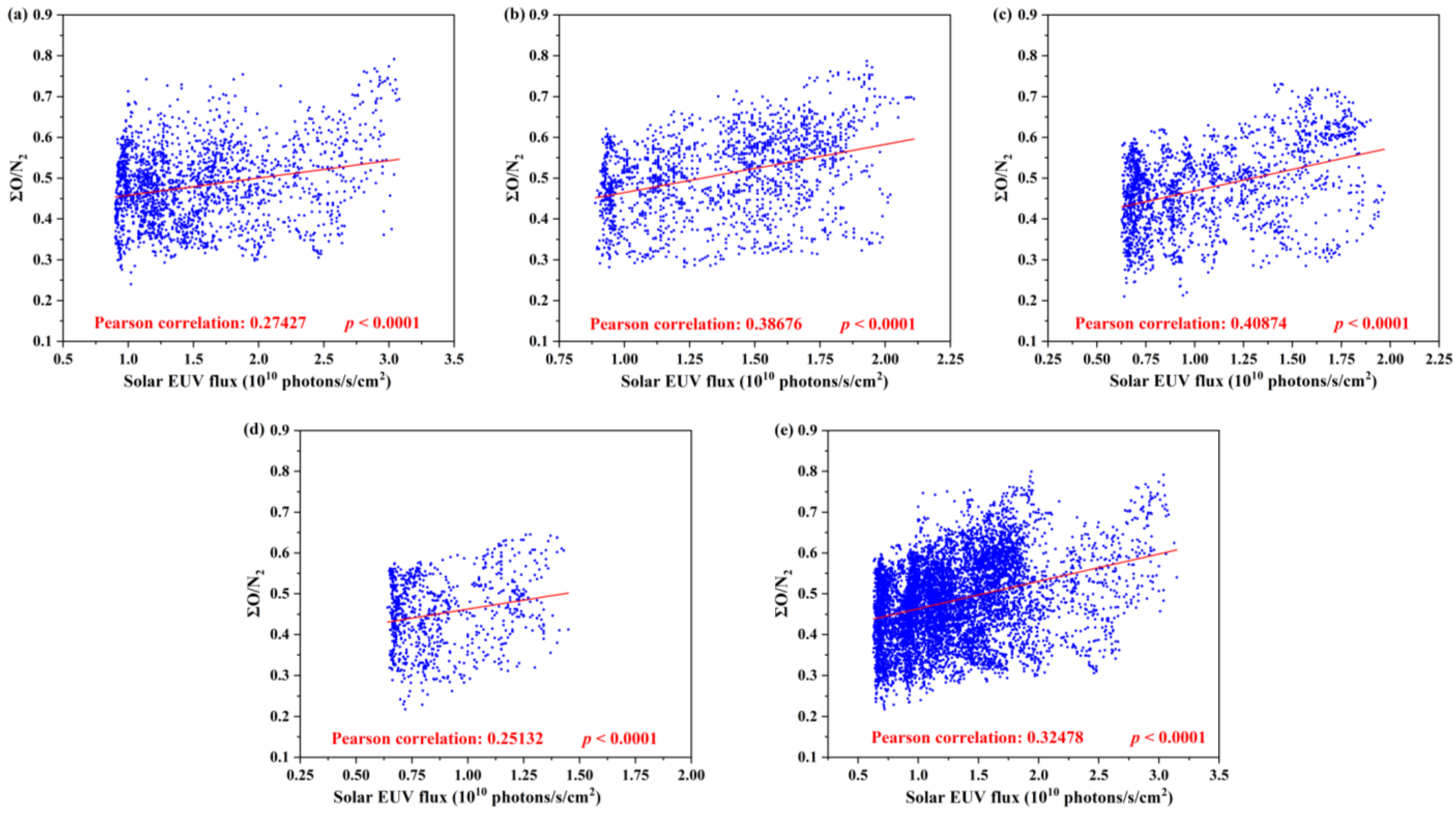
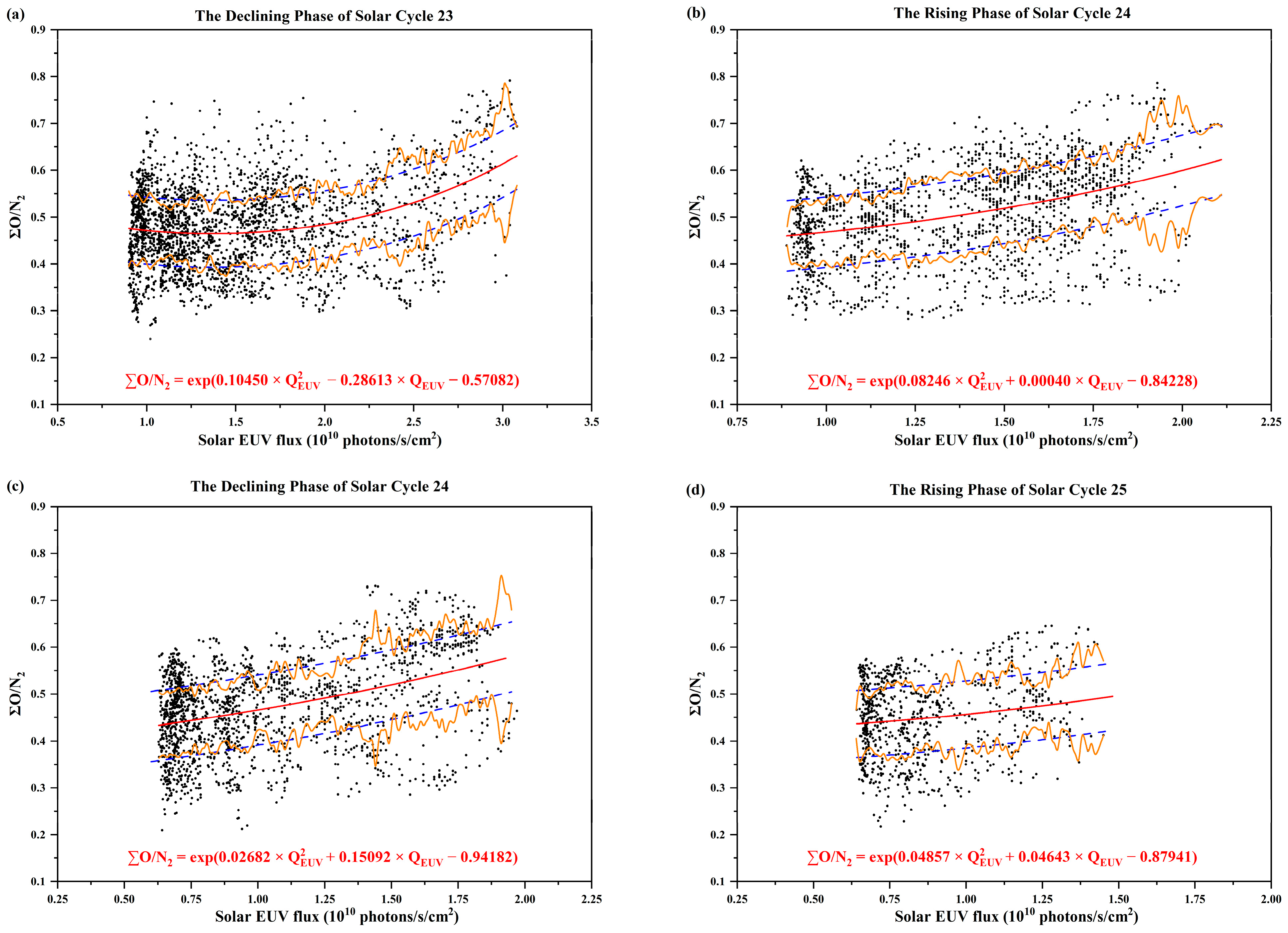
During the declining phase of Solar Cycle 23, throughout Solar Cycle 24, and in the initial phase of Solar Cycle 25, ∑O/N2 and QEUV exhibit a positive correlation. This correlation is mainly due to QEUV influencing atmospheric chemical processes, atmospheric circulation, and wave effects, which, in turn, lead to changes in ∑O/N2.
(2)
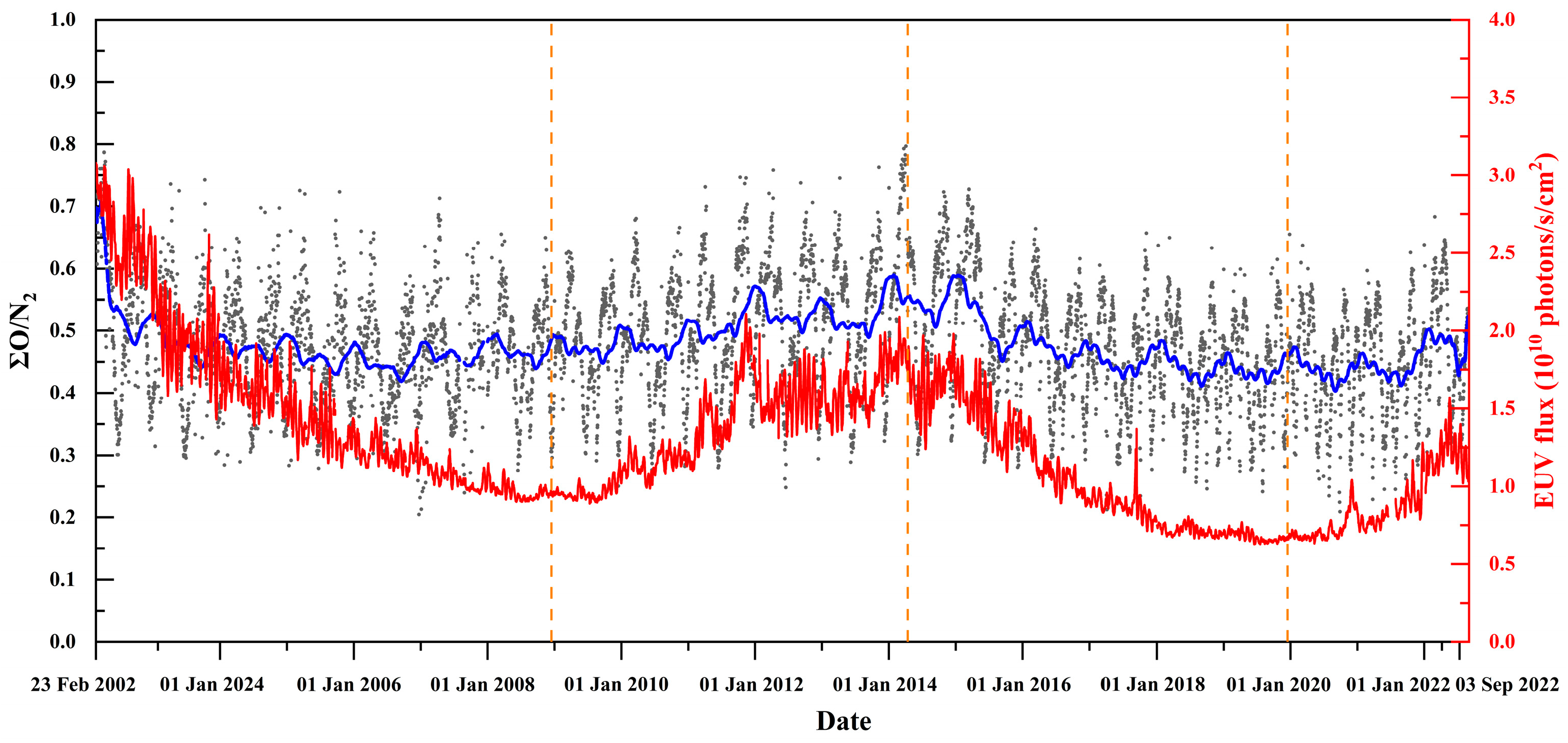
Comparing different solar activity periods, the mean QEUV of Solar Cycle 23 is higher than that of Solar Cycle 24. The mean ∑O/N2 is higher during the rising phase of Solar Cycle 24 and lower during the descending phases of Solar Cycle 23 and Solar Cycle 24.
(3)
During the descending phase of Solar Cycle 23 and the entire Solar Cycle 24, the changes in ∑O/N2 caused by QEUV variations reach about 30% of the mean ∑O/N2 during the same period.
(4)
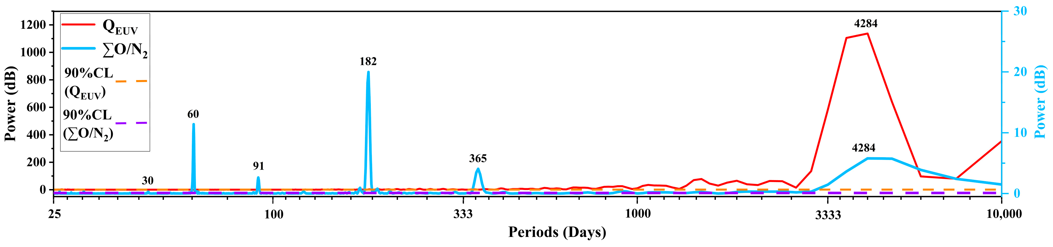
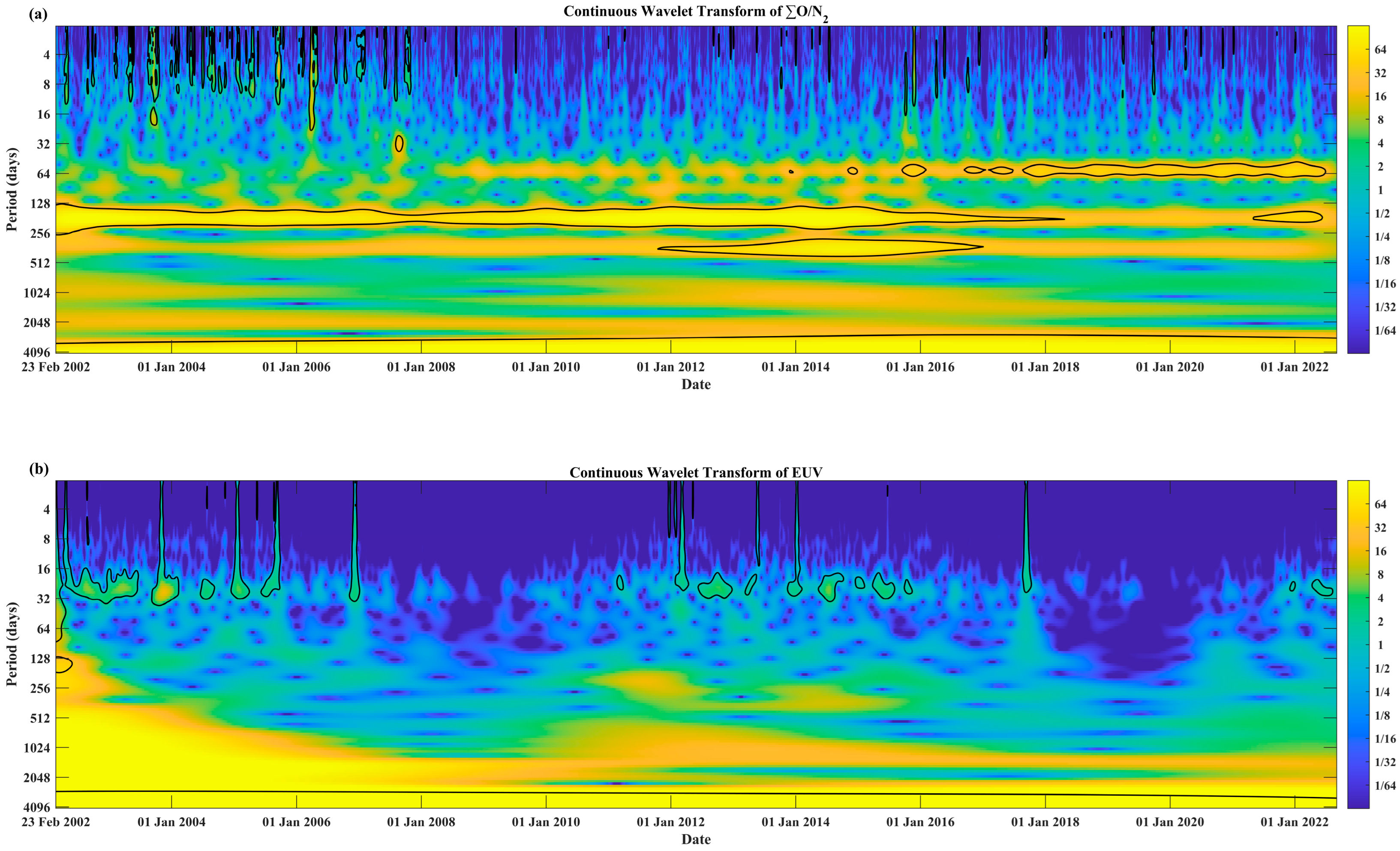
The periodic components with higher coherence between ∑O/N2 and QEUV include the 27-day, annual, and 11-year periodic components. During the rising phase of Solar Cycle 24, the coherence between the annual components is stronger.
This research explored the relationship between QEUV and ∑O/N2, enhancing our understanding of the Sun–Earth system coupling, which is crucial for investigating the effects of solar radiation on the atmosphere of Earth. Analyzing the relationship between the periodic components of QEUV and ∑O/N2 is of significant importance for predicting the potential impact of space weather events on thermospheric composition.

Author Contributions

Conceptualization, H.L. and C.X.; methodology, H.L. and C.X.; software, H.L.; validation, H.L., C.X., X.W., L.X., Z.W. and Y.Y.; formal analysis, H.L.; investigation, C.X. and H.L.; resources, H.L., C.X., Z.W. and Y.Y.; data curation, L.X. and X.W.; writing—original draft preparation, H.L.; writing—review and editing, H.L., C.X. and K.L.; visualization, H.L.; supervision, C.X. and K.L.; project administration, C.X.; funding acquisition, C.X. All authors have read and agreed to the published version of the manuscript.

Funding

This research is funded by the National Natural Science Foundation of China, Grant Nos. 12241101, 42174192, and 91952111.

Data Availability Statement

The ∑O/N2 data used in this study were provided by The Aerospace Corporation and Johns Hopkins University for supporting the data of TIMED/GUVI, which are publicly available at https://guvitimed.jhuapl.edu (accessed on 20 November 2024). The QEUV data were obtained from SOHO, a collaborative international project between ESA and NASA (https://soho.nascom.nasa.gov/home.html (accessed on 24 November 2024)). Information on the solar cycle was provided by the Royal Observatory of Belgium (https://www.sidc.be/SILSO/home (accessed on 11 December 2024)). The wavelet transform and coherence analysis package was provided by Grinsted et al. (http://www.glaciology.net/wavelet-coherence (accessed on 25 December 2024)).

Acknowledgments

The authors sincerely thank Shuo Yao from the China University of Geosciences (Beijing), Jiuhou Lei from the University of Science and Technology of China and Tingting Yu from the Institute of Geology and Geophysics, Chinese Academy of Sciences, for their insightful suggestions on this research. Thanks also go to the reviewers for their comments and suggestions regarding this study.

Conflicts of Interest

The authors declare no conflicts of interest. This research was funded by the National Natural Science Foundation of China, but the funders had no role in the design of the study; in the collection, analysis, or interpretation of data; in the writing of the manuscript; or in the decision to publish the results.

Abbreviations

The following abbreviations are used in this manuscript:
∑O/N2Column O/N2 ratio
QEUVSolar extreme ultraviolet radiation flux
EUVExtreme ultraviolet
GUVIGlobal Ultraviolet Imager
TIMEDThermosphere, Ionosphere, Mesosphere Energetics and Dynamics
SEMSolar EUV Monitor
SOHOSolar and Heliospheric Observatory
LBHLyman–Birge Hopfield bands
LBHSLBH short band
LBHLLBH long band
LTLocal time
TEXOExospheric temperature
FUVFar ultraviolet

References

  1. Strickland, D.J.; Evans, J.S.; Paxton, L.J. Satellite remote sensing of thermospheric O/N2 and solar EUV: 1. Theory. J. Geophys. Res. Space Phys. 1995, 100, 12217–12226. [Google Scholar] [CrossRef]
  2. Zhang, Y.; Paxton, L.J.; Morrison, D.; Wolven, B.; Kil, H.; Meng, C.; Mende, S.B.; Immel, T.J. O/N2 changes during 1–4 October 2002 storms: IMAGE SI-13 and TIMED/GUVI observations. J. Geophys. Res. Space Phys. 2004, 109, A10308. [Google Scholar] [CrossRef]
  3. Crowley, G.; Reynolds, A.; Thayer, J.P.; Lei, J.; Paxton, L.J.; Christensen, A.B.; Zhang, Y.; Meier, R.R.; Strickland, D.J. Periodic modulations in thermospheric composition by solar wind high-speed streams. Geophys. Res. Lett. 2008, 35, L21106. [Google Scholar] [CrossRef]
  4. Khan, J.; Younas, W.; Khan, M.; Amory-Mazaudier, C. Climatology of O/N2 Variations at Low-and Mid-Latitudes during Solar Cycles 23 and 24. Atmosphere 2022, 13, 1645. [Google Scholar] [CrossRef]
  5. Yu, T.; Cai, X.; Ren, Z.; Li, S.; Pedatella, N.; He, M. Investigation of the ΣO/N2 depletion with latitudinally tilted equatorward boundary observed by GOLD during the geomagnetic storm on April 20, 2020. J. Geophys. Res. Space Phys. 2022, 127, e2022JA030889. [Google Scholar] [CrossRef]
  6. Cai, X.; Burns, A.G.; Wang, W.; Qian, L.; Solomon, S.C.; Eastes, R.W.; McClintock, W.E.; Laskar, F.I. Investigation of a neutral “tongue” observed by GOLD during the geomagnetic storm on May 11, 2019. J. Geophys. Res. Space Phys. 2021, 126, e2020JA028817. [Google Scholar] [CrossRef]
  7. Zhang, X.X.; Wang, C.; Chen, T.; Wang, Y.L.; Tan, A.; Wu, T.S.; Germany, G.A.; Wang, W. Global patterns ofJoule heating in the high-latitude ionosphere. J. Geophys. Res. 2005, 110, A12208. [Google Scholar] [CrossRef]
  8. Qian, L.; Yu, W.; Pedatella, N.; Yue, J.; Wang, W. Hemispheric asymmetry of the annual and semiannual variation of thermospheric composition. J. Geophys. Res. Space Phys. 2023, 128, e2022JA031077. [Google Scholar] [CrossRef]
  9. Yu, T.; Ren, Z.; Le, H.; Wan, W.; Wang, W.; Cai, X.; Li, X. Seasonal variation of O/N2 on different pressure levels from GUVI limb measurements. J. Geophys. Res. Space Phys. 2020, 125, e2020JA027844. [Google Scholar] [CrossRef]
  10. Qian, L.; Solomon, S.C.; Kane, T.J. Seasonal variation of thermospheric density and composition. J. Geophys. Res. Space Phys. 2009, 114, A01312. [Google Scholar] [CrossRef]
  11. Zhang, Y.; England, S.; Paxton, L.J. Thermospheric composition variations due tononmigrating tides and their effect on ionosphere. Geophys. Res. Lett. 2010, 37, L17103. [Google Scholar] [CrossRef]
  12. Burns, A.G.; Killeen, T.L.; Wang, W.; Roble, R.G. The solar-cycle-dependent response of the thermosphere to geomagnetic storms. J. Atmos. Sol. Terr. Phys 2004, 66, 1–14. [Google Scholar] [CrossRef]
  13. Floyd, L.; Newmark, J.; Cook, J.; Herring, L.; McMullin, D. Solar EUV and UV spectral irradiances and solar indices. J. Atmos. Sol.-Terr. Phys. 2005, 67, 3–15. [Google Scholar] [CrossRef]
  14. Thiemann, E.M.B.; Dominique, M. PROBA2 LYRA occultations: Thermospheric temperature and composition, sensitivity to EUV forcing, and comparisons with Mars. J. Geophys. Res. Space Phys. 2021, 126, e2021JA029262. [Google Scholar] [CrossRef]
  15. Evans, J.S.; Strickland, D.J.; Huffman, R.E. Satellite remote sensing of thermospheric O/N2 and solar EUV: 2. Data analysis. J. Geophys. Res. Space Phys. 1995, 100, 12227–12233. [Google Scholar] [CrossRef]
  16. Meier, R.R.; Picone, J.M.; Drob, D.; Bishop, J.; Emmert, J.T.; Lean, J.L.; Stephan, A.W.; Strickland, D.J.; Christensen, A.B.; Paxton, L.J.; et al. Remote sensing of Earth’s limb by TIMED/GUVI: Retrieval of thermospheric composition and temperature. Earth Space Sci. 2015, 2, 1–37. [Google Scholar] [CrossRef]
  17. Zhang, Y.; Paxton, L.J. Long-term variation in the thermosphere: TIMED/GUVI observations. J. Geophys. Res. Space Phys. 2011, 116, A00H02. [Google Scholar] [CrossRef]
  18. Smith, A.K.; Marsh, D.R.; Mlynczak, M.G.; Mast, J.C. Temporal variations of atomic oxygen in the upper mesosphere from SABER. J. Geophys. Res. Atmos. 2010, 115, D18309. [Google Scholar] [CrossRef]
  19. Fuller-Rowell, T.J. The “thermospheric spoon”: A mechanism for the semiannual density variation. J. Geophys. Res. Space Phys. 1998, 103, 3951–3956. [Google Scholar] [CrossRef]
  20. Akmaev, R.A. Simulation of large-scale dynamics in the mesosphere and lower thermosphere with the Doppler-spread parameterization of gravity waves: 1. Implementation and zonal mean climatologies. J. Geophys. Res. Atmos. 2001, 106, 1193–1204. [Google Scholar] [CrossRef]
  21. Akmaev, R.A. Simulation of large-scale dynamics in the mesosphere and lower thermosphere with the Doppler-spread parameterization of gravity waves: 2. Eddy mixing and the diurnal tide. J. Geophys. Res. Atmos. 2001, 106, 1205–1213. [Google Scholar] [CrossRef]
  22. Meier, R.R. The thermospheric column O/N2 ratio. J. Geophys. Res. Space Phys. 2021, 126, e2020JA029059. [Google Scholar] [CrossRef]
  23. Strickland, D.J.; Evans, J.S.; Correira, J. Comment on “Long-term variation in the thermosphere: TIMED/GUVI observations” by Y. Zhang and L.J. Paxton. J. Geophys. Res. Space Phys. 2012, 117, A07302. [Google Scholar] [CrossRef]
  24. Comberiate, J.; Paxton, L.J. Global Ultraviolet Imager equatorial plasma bubble imaging and climatology, 2002–2007. J. Geophys. Res. Space Phys. 2010, 115, A04305. [Google Scholar] [CrossRef]
  25. Kamalabadi, F.; Comberiate, J.M.; Taylor, M.J.; Pautet, P.-D. Estimation of electron densities in the lower thermosphere from GUVI 135.6 nm tomographic inversions in support of SpreadFEx. Ann. Geophys. 2009, 27, 2439–2448. [Google Scholar] [CrossRef]
  26. Christensen, A.B.; Paxton, L.J.; Avery, S.; Craven, J.; Crowley, G.; Humm, D.C.; Kil, H.; Meier, R.R.; Meng, C.I.; Morrison, D.; et al. Initial observations with the Global Ultraviolet Imager (GUVI) in the NASA TIMED satellite mission. J. Geophys. Res. Space Phys. 2003, 108, 553–559. [Google Scholar] [CrossRef]
  27. Paxton, L.J.; Christensen, A.B.; Humm, D.C.; Ogorzalek, B.S.; Pardoe, C.T.; Morrison, D.; Weiss, M.B.; Crain, W.; Lew, P.H.; Mabry, D.J.; et al. Global ultraviolet imager (GUVI): Measuring composition and energy inputs for the NASA Thermosphere Ionosphere Mesosphere Energetics and Dynamics (TIMED) mission. Proc. SPIE Int. Soc. Opt. Eng. 1999, 3756, 265–276. [Google Scholar] [CrossRef]
  28. Strickland, D.J.; Meier, R.R.; Walterscheid, R.L.; Craven, J.D.; Christensen, A.B.; Paxton, L.J.; Morrison, D.; Crowley, G. Quiet-time seasonal behavior of the thermosphere seen in the far ultraviolet dayglow. J. Geophys. Res. Space Phys. 2004, 109, A01302. [Google Scholar] [CrossRef]
  29. Roble, R.G. Energetics of the mesosphere and thermosphere. In The Upper Mesosphere and Lower Thermosphere: A Review of Experiment and Theory; Springer: Dordrecht, The Netherlands, 1995; pp. 1–21. [Google Scholar] [CrossRef]
  30. Hovestadt, D.; Hilchenbach, M.; Bürgi, A.; Klecker, B.; Laeverenz, P.; Scholer, M.; Grünwaldt, H.; Axford, W.I.; Livi, S.; Marsch, E.; et al. CELIAS-charge, element and isotope analysis system for SOHO. In The SOHO Mission; Fleck, B., Domingo, V., Poland, A., Eds.; Springer: Dordrecht, The Netherlands, 1995; pp. 159–163. [Google Scholar] [CrossRef]
  31. Judge, D.L.; McMullin, D.R.; Ogawa, H.S.; Hovestadt, D.; Klecker, B.; Hilchenbach, M.; Möbius, E.; Canfield, L.R.; Vest, R.E.; Watts, R.; et al. First Solar EUV Irradiances Obtained from SOHO by the Celias/Sem. Sol. Phys. 1998, 177, 161–173. [Google Scholar] [CrossRef]
  32. Judge, D.L.; McMullin, D.R.; Ogawa, H.S. Absolute solar 30.4 nm flux from sounding rocket observations during the solar cycle 23 minimum. J. Geophys. Res. Space Phys. 1999, 104, 28321–28324. [Google Scholar] [CrossRef]
  33. Judge, D.; Ogawa, H.; McMullin, D.; Gangopadhyay, P.; Pap, J. The SOHO CELIAS/SEM EUV database from SC23 minimum to the present. Adv. Space Res. 2002, 29, 1963–1968. [Google Scholar] [CrossRef]
  34. Yu, T.; Ren, Z.; Yu, Y.; Yue, X.; Zhou, X.; Wan, W. Comparison of reference heights of O/N2 and ∑O/N2 based on GUVI dayside limb measurement. Space Weather. 2020, 18, e2019SW002391. [Google Scholar] [CrossRef]
  35. Dang, T.; Wang, W.; Burns, A.; Dou, X.; Wan, W.; Lei, J. Simulations of the ionospheric annual asymmetry: Sun-Earth distance effect. J. Geophys. Res. Space Phys. 2017, 122, 6727–6736. [Google Scholar] [CrossRef]
  36. Lei, J.; Dou, X.; Burns, A.; Wang, W.; Luan, X.; Zeng, Z.; Xu, J. Annual asymmetry in thermospheric density: Observations and simulations. J. Geophys. Res. Space Phys. 2013, 118, 2503–2510. [Google Scholar] [CrossRef]
  37. Yue, J.; Jian, Y.; Wang, W.; Meier, R.; Burns, A.; Qian, L.; Jones, M.; Wu, D.L.; Mlynczak, M. Annual and semiannual oscillations of thermospheric composition in TIMED/GUVI limb measurements. J. Geophys. Res. Space Phys. 2019, 124, 3067–3082. [Google Scholar] [CrossRef]
  38. Jones, M., Jr.; Emmert, J.T.; Drob, D.P.; Picone, J.M.; Meier, R.R. Origins of the thermosphere-ionosphere semiannual oscillation: Reformulating the “thermospheric spoon” mechanism. J. Geophys. Res. Space Phys. 2018, 123, 931–954. [Google Scholar] [CrossRef]
  39. Gasperini, F.; Hagan, M.E.; Zhao, Y. Evidence of tropospheric 90-day oscillations in the thermosphere. Geophys. Res. Lett. 2017, 44, 10125–10133. [Google Scholar] [CrossRef]
  40. Gasperini, F.; Liu, H.; Gan, Q. Madden-Julian Oscillation (MJO) Effects in the GOLD O/N2 and Swarm-C neutral density during 2018–2019? ESS Open Arch. 2020. [Google Scholar] [CrossRef]
  41. Forbes, J.M.; Bruinsma, S.; Lemoine, F.G. Solar rotation effects on the thermospheres of Mars and Earth. Science 2006, 312, 1366–1368. [Google Scholar] [CrossRef] [PubMed]
  42. Lei, J.; Thayer, J.P.; Forbes, J.M.; Wu, Q.; She, C.; Wan, W.; Wang, W. Ionosphere response to solar wind high-speed streams. Geophys. Res. Lett. 2008, 35, L19105. [Google Scholar] [CrossRef]
  43. Chen, Y.; Liu, L.; Le, H.; Zhang, H. Discrepant responses of the global electron content to the solar cycle and solar rotation variations of EUV irradiance. Earth Planets Space 2015, 67, 80. [Google Scholar] [CrossRef]
  44. Elias, A.G.; de Haro Barbás, B.F.; Medina, F.D.; Zossi, B.S. On the Correlation between EUV Solar Radiation Proxies and their Long-Term Association. In Proceedings of the Thirteenth Workshop “Solar Influences on the Magnetosphere, Ionosphere and Atmosphere”; Bulgarian Academy of Sciences: Sofia, Bulgaria, 2021. e-ISSN 2367-7570. Available online: https://ui.adsabs.harvard.edu/link_gateway/2021simi.conf...20E/doi:10.31401/WS.2021.proc (accessed on 2 February 2025).
  45. Elias, A.G.; Martinis, C.R.; de Haro Barbas, B.F.; Medina, F.D.; Zossi, B.S.; Fagre, M.; Duran, T. Comparative analysis of extreme ultraviolet solar radiation proxies during minimum activity levels. Earth Planet. Phys. 2023, 7, 540–547. [Google Scholar] [CrossRef]
  46. Hussain, A.; Cao, J.; Ali, S.; Ullah, W.; Muhammad, S.; Hussain, I.; Abbas, H.; Hamal, K.; Sharma, S.; Akhtar, M.; et al. Wavelet coherence of monsoon and large-scale climate variabilities with precipitation in Pakistan. Int. J. Climatol. 2022, 42, 9950–9966. [Google Scholar] [CrossRef]
  47. Zhang, Y.; Paxton, L.J. Reply to comment by D.J. Strickland et al. on “Long-term variation in the thermosphere: TIMED/GUVI observations”. J. Geophys. Res. Space Phys. 2012, 117, A07304. [Google Scholar] [CrossRef]
  48. Swenson, G.R.; Vargas, F.; Jones, M.; Zhu, Y.; Kaufmann, M.; Yee, J.H.; Mlynczak, M. Intra-Annual Variation of Eddy Diffusion (kzz) in the MLT, From SABER and SCIAMACHY Atomic Oxygen Climatologies. J. Geophys. Res. Atmos. 2021, 126, e2021JD035343. [Google Scholar] [CrossRef] [PubMed]
  49. Malhotra, G.; Ridley, A.J.; Marsh, D.R.; Wu, C.; Paxton, L.J.; Mlynczak, M.G. Impacts of lower thermospheric atomic oxygen on thermospheric dynamics and composition using the global ionosphere thermosphere model. J. Geophys. Res. Space Phys. 2020, 125, e2020JA027877. [Google Scholar] [CrossRef]
  50. Wang, J.C.; Yue, J.; Wang, W.; Qian, L.; Wu, Q.; Wang, N. The lower thermospheric winter-to-summer meridional circulation: 1. Driving mechanism. J. Geophys. Res. Space Phys. 2022, 127, e2022JA030948. [Google Scholar] [CrossRef]
  51. Judge, D.; Ogawa, H.; McMullin, D.; Gangopadhyay, P. The SoHO CELIAS/SEM data base. Phys. Chem. Earth Part C Sol. Terr. Planet. Sci. 2000, 25, 417–420. [Google Scholar] [CrossRef]
Figure 1. GUVI disk daily mean ∑O/N2 and solar EUV flux between 2002 and 2022. The gray dots correspond to the ∑O/N2 data points, the red line represents the QEUV variation curve, the blue line depicts the ∑O/N2 variation derived from semiannual averaging, and the orange dashed line marks the divisions between four phases (the declining phase of Solar Cycle 23, the rising phase of Solar Cycle 24, the declining phase of Solar Cycle 24, and the rising phase of Solar Cycle 25).
Remotesensing 17 00574 g001
Figure 2. The correlation analysis results between ∑O/N2 and QEUV for different solar activity phases: (a) the declining phase of Solar Cycle 23 (February 2002–December 2008), (b) the rising phase of Solar Cycle 24 (December 2008–April 2014), (c) the declining phase of Solar Cycle 24 (April 2014–December 2019), (d) the rising phase of Solar Cycle 25 (December 2019–September 2022), (e) the results for all periods. The blue dots represent the ∑O/N2 data points, and the red solid line is the fitted curve emphasizing the positive correlation. The two parameters in the figure are the Pearson correlation coefficient and the significance test p-value.
Remotesensing 17 00574 g002
Figure 3. The fitting results of ∑O/N2 and QEUV for different solar cycle phases: (a) the declining phase of Solar Cycle 23 (February 2002–December 2008), (b) the rising phase of Solar Cycle 24 (December 2008–April 2014), (c) the declining phase of Solar Cycle 24 (April 2014–December 2019), and (d) the rising phase of Solar Cycle 25 (December 2019–September 2022). The black dots are the data points, the red line is the fitting function, and the area between the two orange lines represents the influence of other factors on ∑O/N2 for each QEUV value. The blue line indicates the average level of the influence of other factors on ∑O/N2 during that solar activity phase.
Remotesensing 17 00574 g003
Figure 4. Lomb–Scargle periodogram (red line represents QEUV, blue line represents ∑O/N2).
Remotesensing 17 00574 g004
Figure 5. Continuous wavelet transform results: (a) ∑O/N2 wavelet transform result, (b) QEUV wavelet transform result. The colors in the figure represent the signal strength, and the signals within the black contours denote the 95% confidence interval.
Remotesensing 17 00574 g005
Figure 6. Wavelet coherence analysis between ∑O/N2 and QEUV. The arrows in the figure represent the phase information between the two, the color indicates the coherence strength, and the area inside the black contour represents the 95% confidence interval.
Remotesensing 17 00574 g006
Disclaimer/Publisher’s Note: The statements, opinions and data contained in all publications are solely those of the individual author(s) and contributor(s) and not of MDPI and/or the editor(s). MDPI and/or the editor(s) disclaim responsibility for any injury to people or property resulting from any ideas, methods, instructions or products referred to in the content.

