Author Contributions
Conceptualization, Z.W.; methodology, Z.W., Y.L. (Yuhan Liu) and Y.L. (Yuan Li); software, Z.W.; validation, Z.W.; formal analysis, Z.W.; investigation, Z.W.; resources, Z.W.; data curation, Z.W.; writing—original draft preparation, Z.W.; writing—review and editing, Z.W., P.L., Y.L. (Yuhan Liu), J.C., X.X., Y.L. (Yuan Li), H.W., Y.Z. and G.Z.; visualization, Z.W.; supervision, Z.W. and Y.L. (Yuhan Liu). All authors have read and agreed to the published version of the manuscript.
Figure 1.
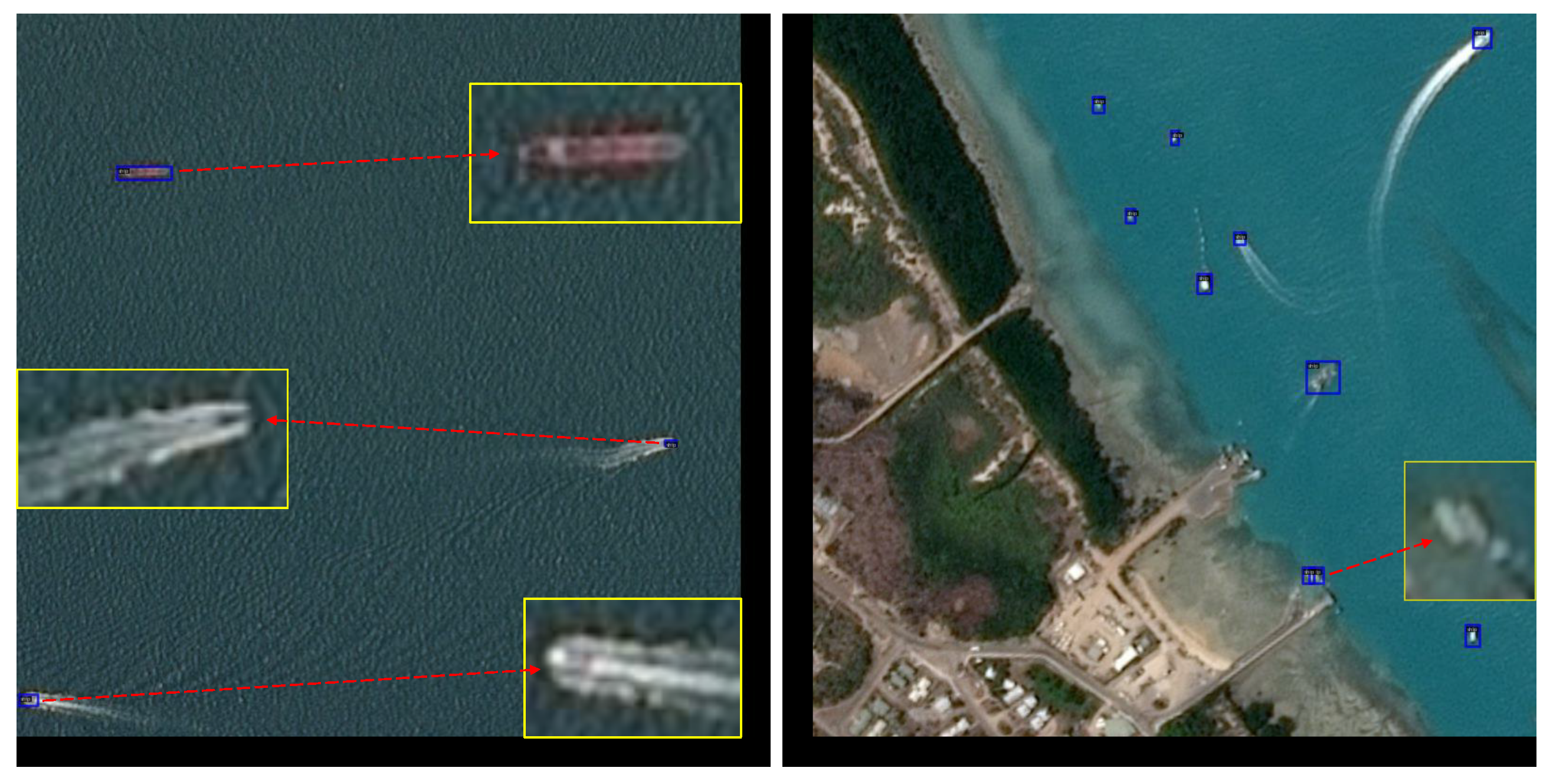
Tiny objects in AI-TOD. (Left): Ships in open sea scenes. (Right): Ships near the port. Due to differences in imaging conditions and backgrounds, objects of the same category exhibit significant intra-class variation.
Figure 1.
Tiny objects in AI-TOD. (Left): Ships in open sea scenes. (Right): Ships near the port. Due to differences in imaging conditions and backgrounds, objects of the same category exhibit significant intra-class variation.
Figure 2.
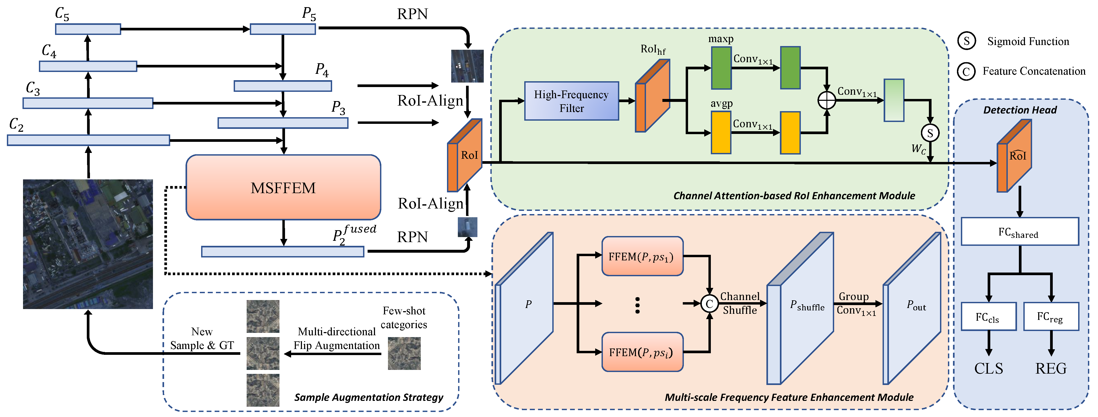
Overview of the proposed FANet. The network is built upon the R-CNN framework, with FPN incorporating the MSFFEM for frequency-domain feature enhancement at the feature map level, and the CAREM for channel attention-based RoI feature refinement at the RoI level. A sample augmentation strategy is employed to balance the training data, improving detection performance for few-shot categories.
Figure 3.
(Left): Remote sensing image containing tiny object in the red box. (Right): Patchwise FFT spectrum visualization. The patch-based FFT reveals that tiny objects exhibit distinctive responses in specific frequency bands, highlighting their spectral characteristics and aiding in discriminative feature extraction.
Figure 4.
Illustration of the FFEM, which divides feature maps into patches, applies frequency-domain filtering, and enhances tiny-object representation.
Figure 4.
Illustration of the FFEM, which divides feature maps into patches, applies frequency-domain filtering, and enhances tiny-object representation.
Figure 5.
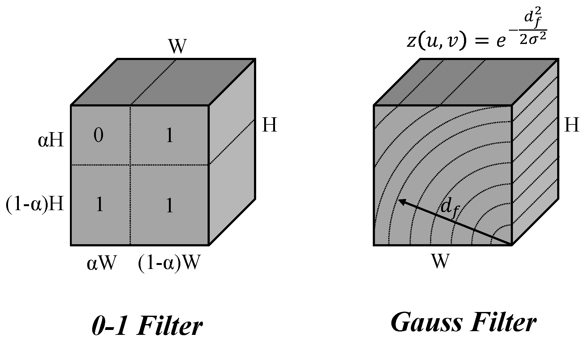
Visualization of the high-frequency filters used in CAREM. (Left): The 0–1 indicator filter. (Right): Gaussian-weighted filter. The Gaussian-weighted filter preserves high-frequency components in the lower-right corner, while the binary indicator filter sharply separates high and low frequencies.
Figure 6.
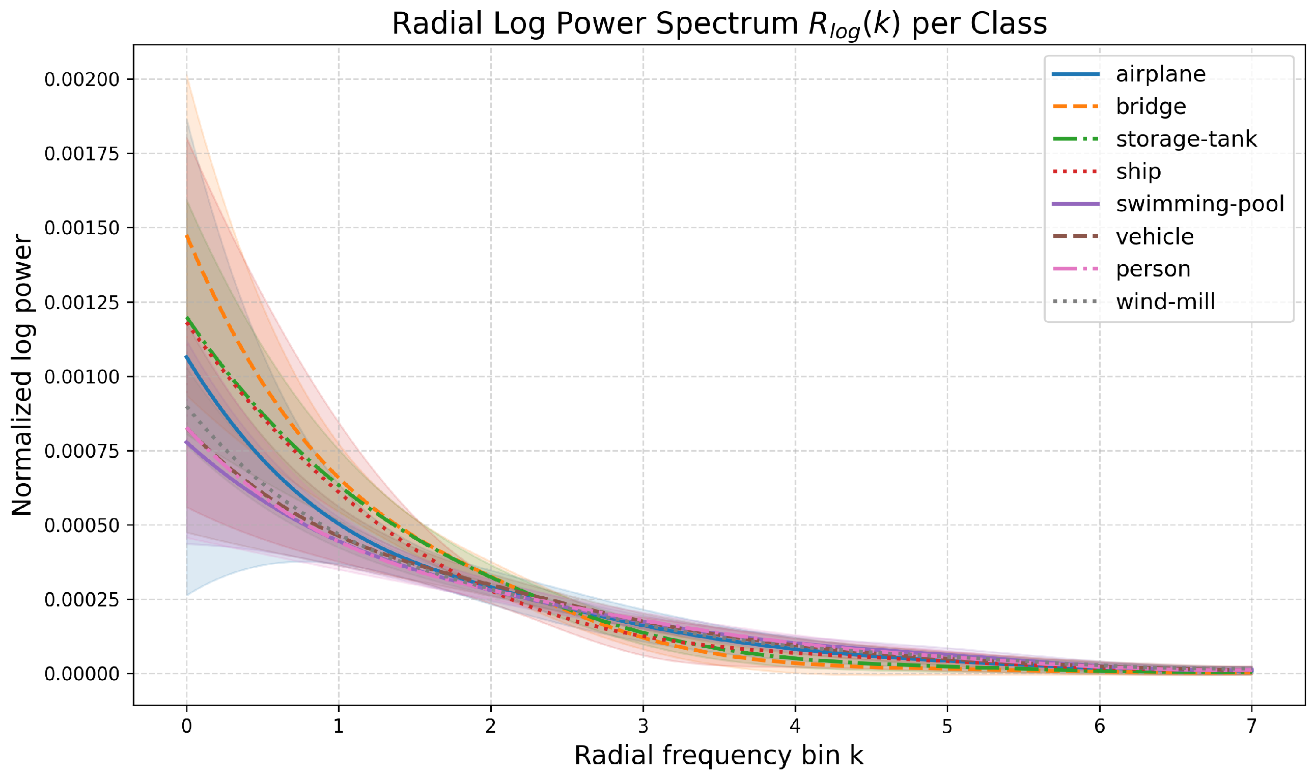
Radially averaged log power spectrum for each object category in the AI-TOD dataset. The colored areas represent the standard deviation range. The results demonstrate significant inter-class differences in frequency-domain distributions.
Figure 6.
Radially averaged log power spectrum for each object category in the AI-TOD dataset. The colored areas represent the standard deviation range. The results demonstrate significant inter-class differences in frequency-domain distributions.
Figure 7.
Visualization of feature maps before and after MSFFEM processing using Eigen-CAM.
Figure 7.
Visualization of feature maps before and after MSFFEM processing using Eigen-CAM.
Figure 8.
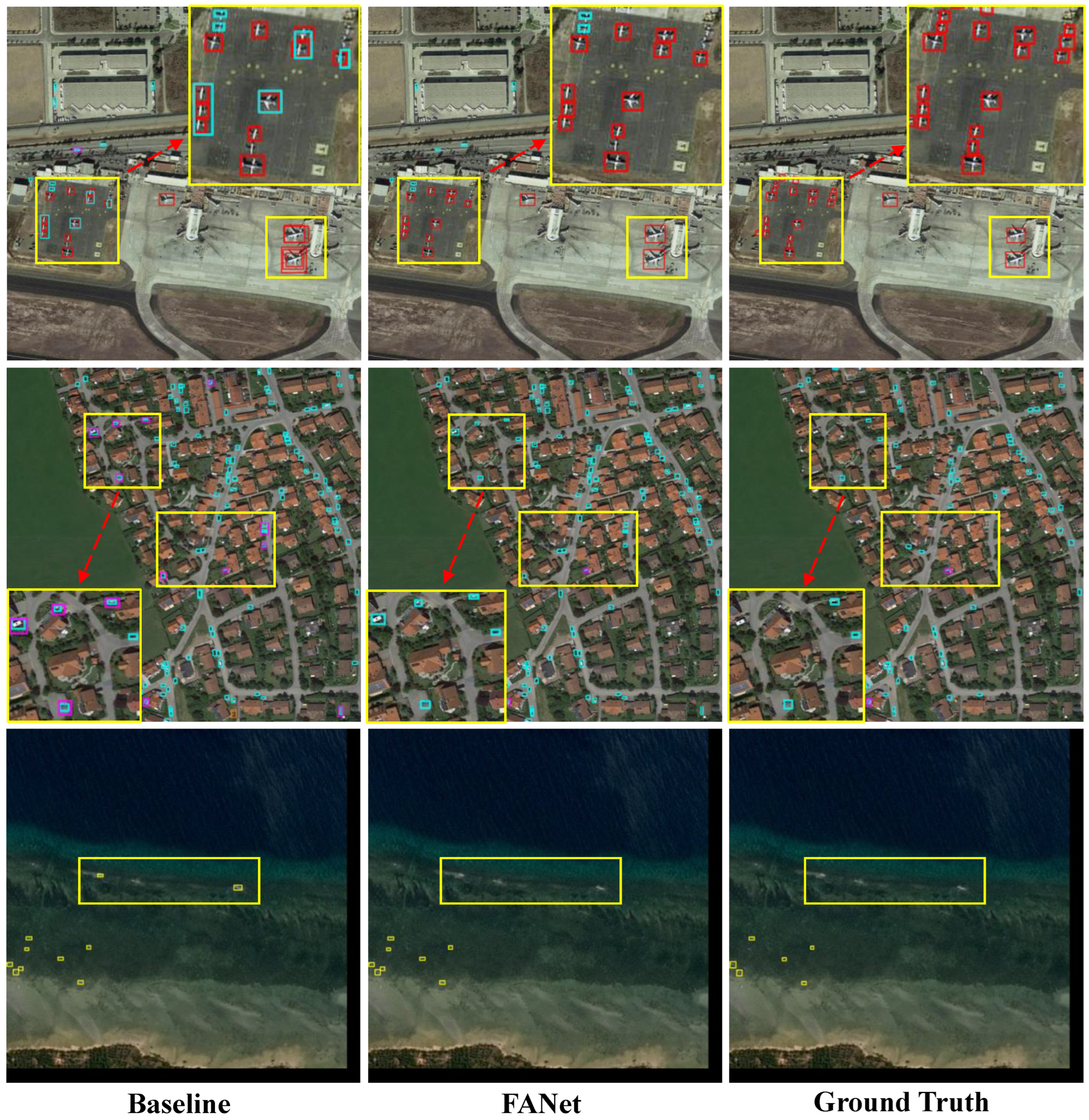
Qualitative comparison of detection results on the AI-TOD test set. From left to right: baseline results, FANet results, and ground truth. Highlighted regions show that FANet produces fewer false positives and more accurate detections compared to the baseline, as frequency-domain enhanced features better emphasize the characteristics of tiny objects and help suppress false alarms.
Figure 9.
Qualitative detection results achieved by our FANet on AI-TOD test set. One color stands for one object class. We could see that FANet demonstrates strong capability in detecting tiny objects with weak features in complex and dense scenes.
Figure 9.
Qualitative detection results achieved by our FANet on AI-TOD test set. One color stands for one object class. We could see that FANet demonstrates strong capability in detecting tiny objects with weak features in complex and dense scenes.
Figure 10.
Qualitative detection results achieved by our FANet on VisDrone2019 val set. One color stands for one object class.
Figure 10.
Qualitative detection results achieved by our FANet on VisDrone2019 val set. One color stands for one object class.
Table 1.
Category proportion and augmentation multiples in the AI-TOD dataset. The category names are abbreviated as follows: AI—airplane, BR—bridge, ST—storage tank, SH—ship, SP—swimming pool, VE—vehicle, PE—person, WM—windmill.
Table 1.
Category proportion and augmentation multiples in the AI-TOD dataset. The category names are abbreviated as follows: AI—airplane, BR—bridge, ST—storage tank, SH—ship, SP—swimming pool, VE—vehicle, PE—person, WM—windmill.
| Category | Percentage Before | Multiple | Percentage After |
|---|
| AI | 0.21 | ×4 | 0.73 |
| BR | 0.20 | ×4 | 0.60 |
| ST | 1.69 | ×2 | 4.09 |
| SH | 5.07 | ×1 | 4.54 |
| SP | 0.08 | ×8 | 0.60 |
| VE | 88.22 | ×1 | 84.85 |
| PE | 4.44 | ×1 | 4.14 |
| WM | 0.08 | ×8 | 0.45 |
Table 2.
Generalization of MSFFEM and CAREM across different methods on the AI-TOD test set. + Ours indicates the integration of both MSFFEM and CAREM. All label assignment methods are based on the Faster R-CNN framework. Floating-point operations per second, parameter counts, and frames per second are reported for each method.
| Method | AP | | | FLOPs | #Params | FPS |
|---|
| Faster R-CNN [7] | 11.1 | 26.3 | 7.6 | 134.42 G | 41.16 M | 45.9 |
| + Ours | 12.1 | 27.9 | 8.7 | 134.65 G | 41.17 M | 37.3 |
| NWD-RKA [35] | 18.8 | 47.5 | 11.1 | 134.42 G | 41.16 M | 40.7 |
| + Ours | 20.1 | 50.1 | 12.0 | 134.65 G | 41.17 M | 38.9 |
| RFLA [36] | 20.6 | 50.4 | 12.9 | 134.42 G | 41.16 M | 42.5 |
| + Ours | 21.4 | 52.4 | 13.4 | 134.65 G | 41.17 M | 38.7 |
| Cascade R-CNN [52] | 13.7 | 30.6 | 10.0 | 162.21 G | 68.95 M | 33.7 |
| + Ours | 13.9 | 31.3 | 10.5 | 162.51 G | 68.97 M | 27.2 |
Table 3.
Ablation study on FFEM and multi-scale (MS) feature fusion. Results in bold indicate the best.
Table 3.
Ablation study on FFEM and multi-scale (MS) feature fusion. Results in bold indicate the best.
| FFEM | MS | AP | | | | | | |
|---|
| - | - | 20.6 | 50.4 | 12.9 | 7.0 | 20.8 | 25.7 | 32.1 |
| ✓ | - | 21.2 | 51.8 | 13.5 | 8.0 | 21.5 | 26.0 | 32.5 |
| ✓ | ✓ | 21.0 | 51.0 | 13.5 | 8.9 | 21.3 | 26.3 | 33.1 |
Table 4.
Ablation study on patch size hyperparameter. Results in bold indicate the best.
Table 4.
Ablation study on patch size hyperparameter. Results in bold indicate the best.
| Patch | AP | | | | | | |
|---|
| - | 20.6 | 50.4 | 12.9 | 7.0 | 20.8 | 25.7 | 32.1 |
| 10 | 20.4 | 50.5 | 12.7 | 8.8 | 20.4 | 25.4 | 32.6 |
| 25 | 20.6 | 50.2 | 13.0 | 9.1 | 20.7 | 25.4 | 32.7 |
| 50 | 21.2 | 51.8 | 13.5 | 8.0 | 21.5 | 26.0 | 32.5 |
| 100 | 21.0 | 51.2 | 13.2 | 7.6 | 21.1 | 26.0 | 32.9 |
Table 5.
Effect of frequency enhancement on different FPN levels. Results in bold indicate the best.
Table 5.
Effect of frequency enhancement on different FPN levels. Results in bold indicate the best.
| Level | AP | | | | | | |
|---|
| - | 20.6 | 50.4 | 12.9 | 7.0 | 20.8 | 25.7 | 32.1 |
| {P2} | 21.2 | 51.8 | 13.5 | 8.0 | 21.5 | 26.0 | 32.5 |
| {P2, P3} | 20.9 | 50.8 | 13.3 | 8.1 | 21.2 | 26.0 | 32.6 |
Table 6.
Ablation study of high-frequency filters and channel attention modules (CAMs) on RoI features. Results in bold indicate the best.
Table 6.
Ablation study of high-frequency filters and channel attention modules (CAMs) on RoI features. Results in bold indicate the best.
| Filter | CAM | AP | | | | | | |
|---|
| - | - | 20.6 | 50.4 | 12.9 | 7.0 | 20.8 | 25.7 | 32.1 |
| - | ✓ | 20.9 | 51.4 | 13.0 | 7.8 | 20.8 | 25.8 | 33.0 |
| 0–1 | ✓ | 21.2 | 51.9 | 13.5 | 7.8 | 21.5 | 26.3 | 32.1 |
| Gauss | ✓ | 21.4 | 51.6 | 13.8 | 8.0 | 21.6 | 26.7 | 33.3 |
Table 7.
Impact of Gaussian filter bandwidth () on detection performance. Results in bold indicate the best.
Table 7.
Impact of Gaussian filter bandwidth () on detection performance. Results in bold indicate the best.
| AP | | | | | | |
|---|
| - | 20.6 | 50.4 | 12.9 | 7.0 | 20.8 | 25.7 | 32.1 |
| 0.2 | 21.2 | 52.2 | 13.4 | 8.3 | 21.3 | 26.3 | 32.9 |
| 1 | 21.3 | 52.0 | 13.8 | 8.1 | 21.5 | 26.5 | 32.2 |
| 2 | 21.4 | 51.6 | 13.8 | 8.0 | 21.6 | 26.7 | 33.3 |
| 5 | 21.0 | 51.7 | 13.1 | 8.7 | 21.1 | 26.9 | 32.1 |
| 10 | 20.9 | 51.3 | 13.1 | 7.4 | 21.0 | 26.9 | 32.0 |
Table 8.
Effect of SAS and vehicle instance reduction on detection performance. We report the class-wise detection results with AP metrics under different IoU thresholds. Category abbreviations are defined in
Table 1.
denotes the proportion of retained vehicle samples, and
indicates the corresponding number of vehicle instances. Results in bold indicate the best.
| | AI | BR | ST | SH | SP | VE | PE | WM | AP | | |
|---|
| - | - | 24.0 | 14.9 | 35.5 | 38.7 | 11.1 | 24.3 | 10.4 | 5.8 | 20.6 | 50.4 | 12.9 |
| 100% | 369 k | 32.3 | 20.7 | 36.6 | 38.9 | 22.0 | 24.6 | 9.9 | 10.6 | 24.4 | 58.1 | 16.7 |
| 70% | 296 k | 32.6 | 20.2 | 36.6 | 39.1 | 19.6 | 24.0 | 10.3 | 9.4 | 24.0 | 56.4 | 16.3 |
| 50% | 241 k | 32.1 | 20.2 | 36.1 | 39.2 | 18.9 | 22.9 | 10.5 | 9.3 | 23.6 | 56.0 | 15.9 |
| 20% | 163 k | 32.2 | 20.4 | 36.0 | 40.4 | 19.1 | 21.3 | 10.5 | 8.6 | 23.6 | 55.6 | 16.5 |
Table 9.
Detailed ablations of MSFFEM, CAREM, and SAS on AI-TOD test set. Results in bold indicate the best.
Table 9.
Detailed ablations of MSFFEM, CAREM, and SAS on AI-TOD test set. Results in bold indicate the best.
| MSFFEM | CAREM | SAS | AP | | | | | | |
|---|
| - | - | - | 20.6 | 50.4 | 12.9 | 7.0 | 20.8 | 25.7 | 32.1 |
| ✓ | - | - | 21.0 | 51.0 | 13.5 | 8.9 | 21.3 | 26.3 | 33.1 |
| - | ✓ | - | 21.4 | 51.6 | 13.8 | 8.0 | 21.6 | 26.7 | 33.3 |
| ✓ | ✓ | - | 21.4 | 52.4 | 13.7 | 8.2 | 21.8 | 26.4 | 33.8 |
| - | - | ✓ | 24.4 | 58.1 | 16.7 | 9.0 | 24.7 | 31.0 | 35.0 |
| ✓ | ✓ | ✓ | 24.8 | 58.1 | 17.5 | 10.7 | 24.9 | 31.6 | 34.9 |
Table 10.
Ablation studies on VisDrone2019 and DOTA-v1.5 validation sets. Results in bold indicate the best.
Table 10.
Ablation studies on VisDrone2019 and DOTA-v1.5 validation sets. Results in bold indicate the best.
| MSFFEM | CAREM | VisDrone2019 | DOTA-v1.5 |
|---|
| AP | | | AP | | |
|---|
| - | - | 21.1 | 41.6 | 7.0 | 40.0 | 67.5 | 13.3 |
| ✓ | - | 21.6 | 42.6 | 7.4 | 40.2 | 67.8 | 13.8 |
| - | ✓ | 21.4 | 42.1 | 7.2 | 40.2 | 68.0 | 13.7 |
| ✓ | ✓ | 21.7 | 43.0 | 7.5 | 40.5 | 68.5 | 14.2 |
Table 11.
Comparison of the proposed FANet with previous methods on AI-TOD test set. All methods were trained for 12 epochs. Red denotes the best results, and blue second-best. Note that † indicates method reproduced, ‡ indicates method trained with SAS, and FCOS* means using P2–P6 of FPN.
Table 11.
Comparison of the proposed FANet with previous methods on AI-TOD test set. All methods were trained for 12 epochs. Red denotes the best results, and blue second-best. Note that † indicates method reproduced, ‡ indicates method trained with SAS, and FCOS* means using P2–P6 of FPN.
| Method | Source | Backbone | AP | | | | | | |
|---|
| Anchor-based Method |
| SSD-512 [8] | ECCV2016 | VGG-16 | 7.0 | 21.7 | 2.8 | 1.0 | 4.7 | 11.5 | 13.5 |
| TridentNet [54] | ICCV2019 | ResNet-50 | 7.5 | 20.9 | 3.6 | 1.0 | 5.8 | 12.6 | 14.0 |
| RetinaNet [55] | ICCV2017 | ResNet-50 | 8.7 | 22.3 | 4.8 | 2.4 | 8.9 | 12.2 | 16.0 |
| Faster R-CNN † [7] | TPAMI2017 | ResNet-50 | 11.1 | 26.3 | 7.6 | 0.0 | 7.2 | 23.3 | 33.6 |
| Cascade RPNN [56] | NIPS2019 | ResNet-50 | 13.3 | 33.5 | 7.8 | 3.9 | 12.9 | 18.1 | 26.3 |
| Cascade R-CNN † [52] | CVPR2018 | ResNet-50 | 13.7 | 30.6 | 10.0 | 0.0 | 10.0 | 26.1 | 36.4 |
| DetectoRS [17] | CVPR2021 | ResNet-50 | 14.8 | 32.8 | 11.4 | 0.0 | 10.8 | 28.3 | 38.0 |
| DotD [57] | CVPR2021 | ResNet-50 | 16.1 | 39.2 | 10.6 | 8.3 | 17.6 | 18.1 | 22.1 |
| Anchor-free Method |
| FoveaBox [58] | TIP2020 | ResNet-50 | 8.1 | 19.8 | 5.1 | 0.9 | 5.8 | 13.4 | 15.9 |
| RepPoints [59] | ICCV2019 | ResNet-50 | 9.2 | 23.6 | 5.3 | 2.5 | 9.2 | 12.9 | 14.4 |
| FCOS [60] | ICCV2019 | ResNet-50 | 12.6 | 30.4 | 8.1 | 2.3 | 12.2 | 17.2 | 25.0 |
| FCOS* | ICCV2019 | ResNet-50 | 15.4 | 36.3 | 10.9 | 6.0 | 17.6 | 18.5 | 20.7 |
| CenterNet [61] | ICCV2019 | DLA-34 | 13.4 | 39.2 | 5.0 | 3.8 | 12.1 | 17.7 | 18.9 |
| M-CenterNet [6] | ICPR2021 | DLA-34 | 14.5 | 40.7 | 6.4 | 6.1 | 15.0 | 19.4 | 20.4 |
| FSANet [19] | TGRS2022 | ResNet-50 | 16.3 | 41.4 | 9.8 | 4.4 | 14.6 | 23.4 | 33.3 |
| State-of-the-art Method |
| ORFENet [62] | TGRS2024 | ResNet-50 | 18.9 | 44.4 | 12.7 | 6.9 | 18.4 | 23.4 | 30.3 |
| KLDet [63] | TGRS2024 | ResNet-50 | 19.6 | - | - | 8.4 | 20.6 | 22.7 | 26.4 |
| MENet [25] | TGRS2024 | ResNet-50 | 20.4 | 50.0 | 12.9 | 8.9 | 21.4 | 23.2 | 31.0 |
| Faster R-CNN w/ NWD-RKA † [35] | ISPRS2022 | ResNet-50 | 18.8 | 47.5 | 11.1 | 6.7 | 18.3 | 23.4 | 31.1 |
| Faster R-CNN w/ HS-FPN [44] | AAAI2025 | ResNet-50 | 20.3 | 48.8 | 13.3 | 11.6 | 22.0 | 25.5 | 27.8 |
| Faster R-CNN w/ RFLA † [36] | ECCV2022 | ResNet-50 | 20.6 | 50.4 | 12.9 | 7.0 | 20.8 | 25.7 | 32.1 |
| Faster R-CNN w/ SR-TOD [64] | ECCV2024 | ResNet-50 | 20.6 | 49.8 | 13.2 | 7.1 | 21.3 | 26.3 | - |
| FANet | Ours | ResNet-50 | 21.4 | 52.4 | 13.7 | 8.2 | 21.8 | 26.4 | 33.8 |
| FANet ‡ | Ours | ResNet-50 | 24.8 | 58.1 | 17.5 | 10.7 | 24.9 | 31.6 | 34.9 |
Table 12.
Comparison of detection performance on VisDrone2019 and DOTA-v1.5 validation sets. All methods were trained for 12 epochs. Red denotes the best results, and blue second-best. Results of previous methods were reproduced. Note that FCOS* means using P2–P6 of FPN.
Table 12.
Comparison of detection performance on VisDrone2019 and DOTA-v1.5 validation sets. All methods were trained for 12 epochs. Red denotes the best results, and blue second-best. Results of previous methods were reproduced. Note that FCOS* means using P2–P6 of FPN.
| Method | Source | Backbone | VisDrone2019 | DOTA-v1.5 |
|---|
| AP | | | AP | | |
|---|
| RetinaNet [55] | ICCV2017 | ResNet-50 | 15.1 | 27.9 | 1.5 | 30.0 | 55.6 | 5.6 |
| FCOS [60] | ICCV2019 | ResNet-50 | 17.0 | 32.6 | 3.1 | 35.6 | 61.5 | 8.8 |
| FCOS* | ICCV2019 | ResNet-50 | 18.9 | 36.9 | 5.9 | 33.2 | 58.1 | 10.4 |
| Faster R-CNN [7] | TPAMI2017 | ResNet-50 | 19.1 | 35.3 | 2.3 | 39.9 | 66.5 | 11.1 |
| Cascade R-CNN [52] | CVPR2018 | ResNet-50 | 19.8 | 35.4 | 2.4 | 40.2 | 64.5 | 9.3 |
| DetectoRS [17] | CVPR2021 | ResNet-50 | 21.6 | 38.0 | 2.8 | 41.3 | 65.3 | 10.1 |
| Faster R-CNN w/ NWD-RKA [35] | ISPRS2022 | ResNet-50 | 21.0 | 41.3 | 6.2 | 40.1 | 68.1 | 13.7 |
| Faster R-CNN w/ RFLA [36] | ECCV2022 | ResNet-50 | 21.1 | 41.6 | 7.0 | 40.0 | 67.5 | 13.3 |
| FANet | Ours | ResNet-50 | 21.7 | 43.0 | 7.5 | 40.5 | 68.5 | 14.2 |
