Deep Transfer Learning for UAV-Based Cross-Crop Yield Prediction in Root Crops

Highlights

What are the main findings?

• Two-way ANOVA revealed significant effects of cover crop on sweet potato yield, whereas nitrogen rate and the interaction term were not substantial.
• Cross-crop robustness analysis identified SAVI, OSAVI, EVI, EVI2, DVI, TSAVI, and $V_f$ as the most transferable features between potato and sweet potato.
• The hybrid CNN–RNN–Attention model achieved the highest accuracy, reaching $R^2=0.64$ and RMSE $\approx$ 18% using only seven robust predictors.

What is the implication of the main finding?

• Cover crop selection is a stronger determinant of yield than fertilizer rate, informing management decisions.
• Using physiologically stable, cross-crop robust features improves model generalization and reduces redundancy in transfer learning.
• Efficient, data-sparse UAV-based yield forecasting is feasible, enabling scalable precision agriculture across root and tuber crops.

Abstract

Limited annotated data often constrain accurate yield prediction in underrepresented crops. To address this challenge, we developed a cross-crop deep transfer learning (TL) framework that leverages potato (Solanum tuberosum L.) as the source domain to predict sweet potato (Ipomoea batatas L.) yield using multi-temporal uncrewed aerial vehicle (UAV)-based multispectral imagery. A hybrid convolutional–recurrent neural network (CNN–RNN–Attention) architecture was implemented with a robust parameter-based transfer strategy to ensure temporal alignment and feature-space consistency across crops. Cross-crop feature migration analysis showed that predictors capturing canopy vigor, structure, and soil–vegetation contrast exhibited the highest distributional similarity between potato and sweet potato. In comparison, pigment-sensitive and agronomic predictors were less transferable. These robustness patterns were reflected in model performance, as all architectures showed substantial improvement when moving from the minimal 3 predictor subset to the 5–7 predictor subsets, where the most transferable indices were introduced. The hybrid CNN–RNN–Attention model achieved peak accuracy ($R^2\approx 0.64$ and RMSE ≈ 18%) using time-series data up to the tuberization stage with only 7 predictors. In contrast, convolutional neural network (CNN), bidirectional gated recurrent unit (BiGRU), and bidirectional long short-term memory (BiLSTM) baseline models required 11–13 predictors to achieve comparable performance and often showed reduced or unstable accuracy at higher dimensionality due to redundancy and domain-shift amplification. Two-way ANOVA further revealed that cover crop type significantly influenced yield, whereas nitrogen rate and the interaction term were not significant. Overall, this study demonstrates that combining robustness-aware feature design with hybrid deep TL model enables accurate, data-efficient, and physiologically interpretable yield prediction in sweet potato, offering a scalable pathway for applying TL in other underrepresented root and tuber crops.

1. Introduction

Transfer learning (TL) has emerged as one of the most transformative approaches in modern artificial intelligence (AI). Unlike conventional machine learning, which requires large annotated datasets to train models from scratch, TL enables knowledge gained in one domain (the source) to be reused and adapted to another (the target) [1]. By transferring learned representations, such as spectral, spatial, and agronomic features or temporal growth patterns, TL significantly reduces the amount of labeled data, computational cost, and time required to develop robust predictive models. In fields where high-quality datasets are scarce, expensive, or difficult to obtain, TL offers a practical and powerful solution. In the current era of rapidly expanding data-driven sciences, TL is particularly valuable for addressing domain imbalance, where well-studied systems (e.g., image classification/recognition, crop mapping, and vegetation monitoring) benefit from large-scale datasets while many underrepresented systems remain constrained by limited data availability [2,3,4,5].

In agriculture, TL is increasingly recognized as essential for advancing precision farming and yield forecasting. Studies have demonstrated that TL has proven effective in the classification of crop species across different regions, enhances disease detection under varying stress conditions, and boosts yield prediction accuracy even when training data are limited [5,6,7,8,9]. The current global challenges of resource scarcity and the demand for sustainable intensification of agriculture heighten its relevance. By enabling scalable, data-efficient, and generalizable AI solutions, TL plays a central role in the digital transformation of agriculture.

Sweet potato (Ipomoea batatas, L.), one of the world’s most significant root crops [10], exemplifies a system where TL can play a critical role in overcoming data limitations. It ranks as the seventh most important food crop globally and the fifth most significant in the tropics, with a global production of nearly 89 million metric tons in 2020, more than 55% of which originated from China [11,12]. In the United States, sweet potato production has expanded considerably, rising from 1.3 billion pounds in 2000 to a peak of 3.1 billion pounds in 2015, with North Carolina as the leading producer, contributing an estimated $170 million annually to the national economy [13]. The United States also ranks as the most significant global exporter of sweet potatoes, underscoring its economic importance in international food systems [14]. Beyond its monetary role, sweet potato provides critical nutritional value, serving as a dense source of provitamin A (beta-carotene), which supplies more than 120% of the recommended daily intake per 100 g serving, alongside vitamin C, potassium, manganese, and dietary fiber [11]. Environmentally, the crop is notable for its adaptability to marginal soils, drought tolerance, and high productivity per hectare, positioning it as an essential component of sustainable agricultural systems. This combination of economic significance, nutritional benefits, and environmental resilience highlights sweet potato as a strategic crop for addressing global food and nutrition security.

Despite its agronomic and nutritional importance, precision monitoring and yield forecasting for sweet potato remain underexplored compared to cereals and cash crops. To assess the strengths and limitations of existing crop monitoring approaches, four primary technologies are commonly considered: manual phenotyping [15], Uncrewed Ground Vehicles (UGVs) [16,17], Uncrewed Aerial Vehicles (UAVs) [18], and satellite-based remote sensing [19]. UGVs and manual phenotyping provide high-precision, ground-level measurements, making them well-suited for yield prediction and detailed stress or disease detection. Still, they are labor-intensive, expensive, and limited in spatial coverage [15,17]. UAVs (or drones) offer a balance between resolution and coverage, enabling rapid acquisition of multispectral and hyperspectral imagery for biomass estimation, canopy characterization, and yield forecasting [20]. However, UAV operations are constrained by weather conditions, flight duration, and complex canopy architectures such as those observed in sprawling or root crops like potato and sweet potato. At broader scales, satellite platforms such as Sentinel-2 and Landsat offer long-term, continuous monitoring across diverse agroecosystems. However, their moderate spatial resolution and sensitivity to cloud cover restrict precision at the field level [21]. Comparative analyses indicate that UAVs achieve very high spatial resolution and moderate operational costs. At the same time, satellites offer cost-effective coverage for large areas but moderate accuracy for disease or stress detection. UGVs, despite their precision, are less scalable and more resource-intensive.

Advances in UAV-based remote sensing have enabled high-throughput monitoring of crop growth, yet current “UAV + machine learning” approaches for sweet potato remain limited in feature richness, model complexity, and predictive accuracy. Existing studies on root crops yield prediction typically rely on single or a few vegetation indices (VIs) (i.e., 3–6 VIs) and employ mid-level machine learning models such as random forests, ridge regression, or convolutional neural network (CNN), without incorporating additional agronomic, spatial, or environmental predictors that are often critical for accurate yield modeling [22,23,24]. For example, Singh et al. (2025) [22] used a multispectral VIs set with regression-based models and achieved modest performance ($R^2$ ≈ 0.45–0.60, RMSE > 20%), demonstrating limited ability to capture sweet potato’s complex canopy dynamics. Tedesco et al. (2021) [23] implemented deeper CNN architectures. However, these were applied primarily to postharvest shape and quality traits rather than to UAV-based yield prediction, and they still relied on narrow feature sets. More recently, Liu et al. (2024) [24] modeled sweet potato morphology using 30 engineered agronomic and environmental variables. Still, the approach did not incorporate UAV spectral data and did not address the challenges of canopy occlusion, spectral saturation, and phenological variability. In contrast, related tuber crops such as potato have benefited from more advanced multispectral modeling pipelines that integrate spectral, structural, and agronomic features within context-aware and hybrid deep learning architectures, achieving $R^2$ > 0.70 and RMSE < 15% [20].

Direct transfer of stage specific yield-prediction models developed for other crops [25,26,27] is particularly challenging for root crops like sweet potato and potato. Unlike cereals or upright row crops, their sprawling vine architecture creates irregular canopy geometry, significant within-plot variability, and inconsistent soil–vegetation mixing, all of which degrade feature stability. Their leaves also exhibit substantial spectral similarity to other broadleaf species, making it difficult for pretrained RGB/NIR models to distinguish phenological transitions [28]. Furthermore, because storage roots develop underground, aboveground canopy signals often exhibit weaker or nonlinear relationships with yield than in foliage-dominated crops, limiting the portability of models trained elsewhere. Additionally, the scarcity of large annotated datasets and the labor-intensive nature of root yield measurements restrict the development of robust supervised learning pipelines. Seasonal and regional variability further constrains model generalization, underscoring the need for approaches that can learn efficiently from limited, heterogeneous datasets. TL has emerged as a powerful tool to address such gaps, enabling models trained on data-rich crops to be adapted to underrepresented ones with minimal labeled data [29]. In related tuber crops such as potato, UAV- and hyperspectral-based machine learning models have shown effective predictive performance, and when enriched with cultivar-specific or phenological information, have further improved yield accuracy [20]. These findings suggest an opportunity: could similar cross-crop TL help unlock scalable monitoring frameworks for sweet potato?

Building on this insight, the present study investigates whether potato, structurally and physiologically similar to sweet potato, can serve as a surrogate for pretraining deep learning models. Both crops exhibit broadleaf canopies with overlapping foliage, comparable spectral responses due to shared chlorophyll and mesophyll traits, and tuber biomass strongly linked to canopy development. Agronomically, both are row-planted, sensitive to nitrogen fertilization, and display similar canopy–yield coupling, reinforcing the case for cross-crop transfer. Here, we propose a hybrid deep learning framework (CNN + convolutional neural network (RNN) + Attention) pretrained on potato datasets and fine-tuned on limited sweet potato UAV data. To address canopy irregularity and spectral overlap, we integrate feature engineering to expand vegetation indices and maintain consistent temporal representation. By selectively unfreezing model layers and aligning spectral–temporal features, the framework mitigates structural and spectral ambiguities while enabling yield prediction with reduced reliance on extensive ground-truthing. The study specifically addresses the following research questions:

1.

Can TL effectively overcome the limitations of small, underrepresented datasets for sweet potato yield prediction?

2.

How can canopy irregularity and spectral overlap be mitigated through feature engineering and model design?

3.

Does selective fine-tuning of pretrained models improve yield prediction compared to training from scratch or traditional machine learning approaches?

By addressing these questions, we present a scalable, data-efficient approach for AI-driven yield forecasting in sweet potato. More broadly, this work demonstrates how transfer learning can bridge data gaps for underrepresented crops, advancing the reach of precision agriculture and ensuring that root and tuber crops are not left behind in the era of AI-enabled farming.

2. Materials

2.1. Experimental Field, Design and In Situ Data Collection

The source-domain dataset used for TL was obtained from previously published potato field experiments conducted in 2020 and 2021 at the Hermiston Agricultural Research and Extension Center, Oregon State University (HAREC-OSU), Hermiston, OR, USA [20]. These trials involved potato crops under varying nitrogen fertilization and were supported by UAV-based multispectral imaging. Detailed descriptions of field design, management practices, and environmental conditions are provided in our earlier work [20], and are not repeated here. This dataset was selected because potato and sweet potato share comparable canopy structures, spectral responses, and tuber growth characteristics, making it a suitable pretraining source for transfer learning.

The target-domain experiments on sweet potato were conducted at the Pontotoc Ridge-Flatwoods Branch Experiment Station of Mississippi State University (WGS 84: $89°{00}^{\prime }{23.2}^{″}\mathrm{W},34°{08}^{\prime }{10.0}^{″}\mathrm{N}$), located near Pontotoc, Mississippi (Figure 1a). The designed experiment covered 60 plots (each consisting of 3 rows with row spacing of 1.02 m and 9.14 m in length) arranged in a complete randomized block design. This experiment consisted of five nitrogen fertilization treatments (0 kg/ha, 28 kg/ha, 56 kg/ha, 84 kg/ha, and 112 kg/ha) and three cover crop treatments (wheat, fallow, and crimson clover) (Figure 1b). The factorial design allowed assessment of the interactive effects of nitrogen fertilization and cover cropping on sweet potato growth. The study was conducted over two consecutive growing seasons (2022 and 2023) under identical specifications. In both years, following cover crop termination and soil preparation, sweet potatoes were transplanted using a tractor-mounted mechanical transplanter. The yield data were measured as the number of No. 1 box (18 kg/ha) and the total marketable number of boxes (Tot Mkt, 18 kg/ha), which served as indicators of sweet potato yield for production management. The No. 1 sweet potatoes are a category of firm, well-shaped, and relatively clean sweet potatoes defined by the USDA Agricultural Marketing Service (https://www.ams.usda.gov/grades-standards/sweetpotatoes-grades-and-standards (accessed on 16 June 2025)). The total marketable yield includes sweet potato of all categories.

2.2. UAV Field Imaging and Preprocessing

The sweet potato field multispectral images were acquired using a DJI Phantom 4 quadcopter UAV with a built-in multispectral camera (DJI, Shenzhen, China). The UAV camera was mounted on a gimbal with a controllable tilt range of $-90°$ to $+30°$ and consisted of six 1/2.9″ 2.08 MP CMOS sensors with an image size of $1600\times 1300$ and a $62.7°$ field of view. The sensors included a broadband RGB sensor for visible light imaging and five narrowband monochrome sensors (blue: $450\pm 16$ nm; green: $560\pm 16$ nm; red: $650\pm 16$ nm; red-edge: $730\pm 16$ nm; and NIR: $840\pm 26$ nm). To calibrate images and convert digital counts to reflectance, a calibrated reflectance panel was imaged before and after each flight. Camera operation was automatically synchronized with the UAV’s global navigation satellite system (GNSS; GPS + GLONASS + Galileo).

UAV image acquisition was scheduled to coincide with the significant growth stages of sweet potato, deliberately aligned with the phenological stages used in our previous potato experiments to ensure smooth application of transfer learning. Sweet potatoes grew actively from June through September, and imaging was conducted from mid-June through late September before harvest (

Table 1. Summary of UAV-based multispectral image acquisition dates across growth stages in 2022 and 2023.

Year	Date of Acquisition (mm/dd)
ine 2022	06/23	07/07	07/21	08/03	08/16	08/31	09/13	09/29
2023	06/28	-	07/19	-	08/11	08/24	09/13	09/25
ine Growth Stage	Emergence	Hilling		Tuberization		Bulking		Maturity

). During this period, monthly average low and high temperatures ranged from 19–30 °C (June), 21–32 °C (July), 20–32 °C (August), and 16–29 °C (September), with corresponding precipitation levels of 123, 110, 102, and 93 mm, respectively. UAV missions were conducted on eight dates spanning four months, capturing five phenological stages, namely, emergence, hilling, tuberization, bulking, and maturity, consistent with the growth stages monitored in potato.

UAV flights for remote sensing missions were conducted between 10:30 a.m. and 12:00 p.m. each day, either under clear skies or within conditions that ensured flights could be completed without cloud shadows over the field. The flight altitude was 30 m above the canopy surface, providing high-resolution images (∼3 cm/pixel) for monitoring sweet potato growth. Flight routes were preset using Pix4D Capture software (v. 1.3.1; Pix4D, Lausanne, Switzerland) with an image front overlap of 80% and a side overlap of 70%. The collected images were processed in Pix4DMapper (v. 4.9.0; Pix4D, Lausanne, Switzerland) to generate RGB orthomosaic and multispectral orthomosaic images (green, red, red-edge, and NIR). The orthomosaics were orthorectified to correct for geometric and vignetting distortion. A total of four ground control points (GCPs) were deployed at the four corners of the 0.308 ha study field, corresponding to a density of approximately 13 GCPs/ha, consistent with recommended guidelines for high-accuracy UAV photogrammetry. GCPs were collected with a Trimble TSC7 GPS controller and Trimble R12i GPS receiver, and incorporated into the Pix4DMapper project to ensure orthomosaic accuracy.

2.3. Feature Extraction and Dataset Preparation

The orthomosaics generated from preprocessing provided the basis for extracting plot-level spatial and spectral features. A Python (v3.11.7)-based workflow was developed to automate feature extraction, ensuring consistency across all flight dates and treatments [20]. For each of the 60 plots across two growing seasons (2022 and 2023), a total of 13 input features were selected for extraction, comprising 11 robust vegetation spectral indices, one spatial canopy structural descriptor (mean canopy cover, $V_f$), and one agronomic parameter (nitrogen fertilization, $N_f$). These features are listed in

Table 2. Spectral and Spatial Features extracted from the multispectral bands.

Feature	Formula	Reference
1. SR	${\displaystyle \frac{B5}{B3}}$	[30]
2. MARI	$\left({\displaystyle \frac{1}{B2}}-{\displaystyle \frac{1}{B4}}\right)\times B5$	[31]
3. CHLGR	${\displaystyle \frac{B5}{B2}}-1$	[32]
4. OSAVI	$(1+l){\displaystyle \frac{B5-B2}{B5+B2+l}};l=0.16$	[33]
5. SAVI2	${\displaystyle \frac{B5}{B3+(b/a)}};a=0.01,b=1.43$	[34]
6. MSR	${\displaystyle \frac{B5}{B3}}-1$	[30]
7. TSAVI	${\displaystyle \frac{a(B5-aB3-b)}{aB5+B3-ab+X(1+a^2)}}$	[35]
8. SAVI	${\displaystyle \frac{1.5(B5-B3)}{B5+B3+0.5}}$	[34]
9. EVI	${\displaystyle \frac{2.5(B5-B3)}{(B5+6B3-7.5B1+1)}}$	[36]
10. EVI2	${\displaystyle \frac{2.5(B5-B3)}{(B5+2.4B3+1)}}$	[36]
11. DVI	$B5-B3$	[37]
12. Spatial ($V_f)$	${\displaystyle \frac{V_p}{T_p}}$	[20]
13. Agronomic ($N_f$)	Nitrogen fertilization

Bands: B1 = Blue, B2 = Green, B3 = Red, B4 = Red-Edge, B5 = Near-Infrared. Spectral Features: SR = Simple Ratio, MARI = Modified Anthocyanin Reflectance Index, CHLGR = Chlorophyll Green Index, CC = Canopy cover, OSAVI = Optimized Soil-Adjusted Vegetation Index (SAVI), SAVI2 = Second-Order SAVI, TSAVI = Transformed SAVI, EVI = Enhanced Vegetation Index, EVI2 = Second-Order EVI, DVI = Difference Vegetation Index. Spatial Feature: $V_f$ = Canopy Cover, $V_p$ = Total Vegetation Pixel, and $T_p$ = Total Pixel.

.

Two distinct datasets were constructed to implement the parameter (feature)-based deep transfer learning framework: a potato dataset serving as the source domain and a sweet potato dataset serving as the target domain. The source dataset consisted of $N=264$ samples collected across five phenological stages ($T=5$) with selected $F=13$ robust predictor variables, as shown in Table 2. Importantly, the 11 robust spectral indices were selected using a partial least squares regression (PLSR)-based variable importance in projection (VIP) analysis utilizing source domain datasets, ensuring that only physiologically meaningful and highly informative features were retained for transfer learning. In addition, the spatial canopy cover metric ($V_f$) and the agronomic nitrogen input variable ($N_f$) were included to complement the spectral features by representing canopy structure and management-driven variability, respectively. The final set of spectral indices was ranked according to their VIP-derived importance [20], and this ordering is preserved in Table 2 and illustrated in Figure 2. The dataset was further temporally segmented into five critical growth stages-emergence, hilling, tuberization, bulking, and maturity, each of which was used to develop stage-specific source models.

The target-domain dataset consisted of $N=120$ samples (60 per year), collected at UAV acquisition dates that closely matched the potato growth sampling schedule, yielding a temporal sequence of five time points ($T=5$). The identical set of vegetation indices, canopy structural descriptors, and agronomic variables was extracted from the target-domain crop (i.e., sweet potato). To ensure consistency across features and growth stages, the target-domain data were dimensionally aligned with the source domain, enabling effective and stable transfer learning.

Both datasets were subsequently reshaped into standardized 3D tensors of dimension $(N,T,F)$, where the potato dataset was represented as $X_s\in {\mathbb{R}}^{264\times T\times F}$ and the sweet potato dataset as $X_t\in {\mathbb{R}}^{120\times T\times F}$. To systematically evaluate transferability and robustness, experiments were conducted under varying temporal lengths of and predictor variable sets (F). This experimental design ensured that both datasets were harmonized in feature and temporal structure, enabling rigorous evaluation of how increasing feature complexity and temporal depth influenced performance across baseline CNN and RNN models compared with the hybrid CNN–RNN–Attention framework.

3. Methodology

3.1. Transfer Learning

Transfer learning (TL) enables knowledge gained in one domain to be adapted for another, reducing the need for large labeled datasets and lowering training costs. While traditional TL strategies, such as instance reweighting, parameter fine-tuning, feature representation transfer, and relational learning, are well established [38,39], their agricultural applications have mostly remained within single-crop domains [6,9,40,41,42]. Cross-crop TL, in which models trained on one crop are adapted to another, remains underexplored. Such transfer can be effective when crops share similar canopy structures, spectral characteristics, or growth patterns, and when differences introduced by phenology or management practices are appropriately accounted for. Under these conditions, cross-crop TL has the potential to advance scalable crop monitoring and yield prediction by making models more generalizable across species and growing environments.

3.2. Hybrid Deep Transfer Learning Model Architecture

A hybrid deep learning architecture combining convolutional [43], recurrent [44], and attention mechanisms [45] was employed to exploit both spectral–structural features and temporal dependencies, as illustrated in Figure 3. The model accepts input sequences of shape $(N,T,F)$, where N denotes the number of samples, $T\in (1,2,$ …$,t)$ corresponds to the temporal dimension (UAV flight time points or growth stages), and F represents the number of robust vegetation spectral-structural features. The architecture consisted of a source domain 3-Dimensional (3D) input layer followed by a 1D convolutional neural network (CNN) layer with 64 filters, a kernel size of 1, a stride of 1, and ReLU activation, that extracts local temporal patterns across features and growth stages [46]. The CNN output was passed through a time-distributed dense layer with 64 neurons and Rectified linear unit (ReLU) activation. To capture multi-scale temporal dependencies, two bidirectional recurrent modules were applied in parallel: a bidirectional gated recurrent unit (BiGRU) and a bidirectional long short-term memory network (BiLSTM), both with 32 units per direction and configured with return_sequences = True. The resulting hidden representations were concatenated to form a combined temporal feature sequence for each time step t, as shown in Equation (1).

$$h_t=\mathrm{BiGRU}\left(X_s\right)\oplus \mathrm{BiLSTM}\left(X_s\right)$$

(1)

where $X_s\in {\mathbb{R}}^{(N,T,F)}$ is the source domain 3D input feature vector at time t, $h_t\in {\mathbb{R}}^{128}$ is the hidden state representation, and ⊕ denotes concatenation. To emphasize the most informative temporal features, a self-attention mechanism was applied. Attention scores ($e_t$) and normalized attention weight (${\alpha }_t$) were computed by Equation (2).

$$e_t=v^{\top }tanh(W{h}_t+b),{\alpha }_t={\displaystyle \frac{exp\left(e_t\right)}{{\sum }_{k=1}^{T}exp\left(e_k\right)}}$$

(2)

where W and b are trainable weight and bias parameters, and v is the attention context vector that projects hidden states into a scalar relevance score. Specifically, each hidden state is projected using trainable bias parameters $W\in {\mathbb{R}}^{64\times 128}$, $b\in {\mathbb{R}}^{64}$, and a context vector $v\in {\mathbb{R}}^{64}$ to produce unnormalized attention scores ($e_t$), which are normalized with a softmax function to obtain attention weights ${\alpha }_t\in [0,1]$, ensuring ${\sum }_{t=1}^T{\alpha }_t=1$ (Equation (2)). The attention-weighted sequence is aggregated using a GlobalMaxPooling1D layer, yielding a fixed-length context vector $c\in {\mathbb{R}}^{128}$ that summarizes the most informative temporal features. Finally, c is passed through a dense regression layer to generate the yield prediction (Equation (3)).

$$\hat{y}=f\left(c\right),c=\sum _{t=1}^T{\alpha }_t{h}_t,$$

(3)

To extend the hybrid model from the source domain to the target domain, we employed a parameter-based transfer learning approach. For each addition of growth stages, a stage-specific source-domain model was first trained on potato datasets using the hybrid CNN–RNN–attention architecture above. The resulting pretrained model defines a mapping by Equation (4).

$${\hat{y}}_s=f_{{\theta }_s}\left(c\right),$$

(4)

where ${\theta }_s$ denotes the set of parameters of the convolutional, recurrent, attention, and original regression layers learned from the source-domain inputs $X_s\in {\mathbb{R}}^{(N,T,F)}$, c is the attention-weighted context vector, and ${\hat{y}}_s$ is the predicted yield in the source domain. In the transfer learning phase, the source-model parameters were partitioned into frozen and trainable subsets as expressed by Equation (5).

$${\theta }_t=\{{\theta }_s^{\mathrm{frozen}},{\theta }_t^{\mathrm{trainable}}\},$$

(5)

where ${\theta }_s^{\mathrm{frozen}}$ comprises all convolutional, recurrent, and attention-layer weights of the pretrained feature extractor, and ${\theta }_t^{\mathrm{trainable}}$ denotes the parameters of a newly added regression head. Concretely, the original output layer of the source model was replaced by a new head consisting of a dropout layer (rate $=0.3$), a dense hidden layer with 64 units and ReLU activation, and a final linear output neuron. During fine-tuning on the target-domain (sweet potato) dataset, only ${\theta }_t^{\mathrm{trainable}}$ was updated, while ${\theta }_s^{\mathrm{frozen}}$ remained fixed, thereby leveraging rich spectral–temporal representations learned in the source domain and reducing the risk of overfitting on the smaller target dataset. Thus, the resulting target-domain prediction model can be written as:

$${\hat{y}}_t=f_{{\theta }_t}\left(c\right),c=\sum _{t=1}^T{\alpha }_t{h}_t,$$

(6)

where c is the attention-weighted context vector obtained from the frozen feature extractor, and ${\hat{y}}_t$ is the yield prediction for the target crop.

3.3. Hyperparameter, Training, Validation, and Testing

All architectural and training hyperparameters used for both the source-domain and transfer-learning models are summarized in Supplementary File (Table S1). For each component, we report the final values used in the experiments and range of candidate explored during hyperparameter calibration. Architectural parameters such as CNN filter sizes, recurrent layer dimensions, and attention formulation were fixed a priori based on preliminary experiments and domain knowledge. In contrast, hyperparameters related to training and testing (e.g., learning rate, dropout rate, dense-layer size) were optimized via random search.

The dataset was randomly partitioned into training (70%) and testing (30%) subsets using a shuffled split with a fixed random seed (random state = 42). Within the training set, 10% was reserved for validation during model fitting. Hyperparameters were tuned using a random search strategy, which is widely used in deep learning due to its efficiency in high-dimensional search spaces compared to exhaustive grid search [47]. The random search explored learning rates in the range ${10}^{-5}$ to ${10}^{-3}$ (log-uniform sampling), batch sizes of {4, 8, 16, 32}, dropout rates between 0.1 and 0.5, dense-layer sizes of {32, 64, 128}, candidate activation functions {ReLU, GeLU: Gaussian error linear unit, Tanh, Sigmoid}, early stopping patience values in {150, 200, 250}, and maximum epoch limits of {300, 400, 500, 600}. The optimal configuration obtained from this search consisted of a batch size of 8, a maximum of 600 training epochs (with early stopping), and the Adam optimizer with a learning rate of $5\times {10}^{-4}$. The Adam optimizer was chosen for its balance of stability and convergence speed, particularly advantageous in transfer learning scenarios. The training objective was to minimize the mean squared error (MSE) loss defined in Equation (7).

$$\mathcal{L}\left({\theta }_t\right)={\displaystyle \frac{1}{N_t}}\sum _{i=1}^{N_t}{\left(y_{t,i}-{\hat{y}}_{t,i}\right)}^2,$$

(7)

where $y_{t,i}$ and ${\hat{y}}_{t,i}$ represent the true and predicted yields for the ith sample in the target dataset. Importantly, only ${\theta }_t$ (the parameters of the regression head) were updated during backpropagation, while ${\theta }_s^{\mathrm{frozen}}$ (the pretrained convolutional, recurrent, and attention-based parameters from the source domain) remained fixed. To ensure robust adaptation on the limited target dataset, training was governed by an early stopping mechanism (patience = 200 epochs, with best weights restored). In addition to early stopping, dropout regularization (rate = 0.3) and Min–Max feature scaling were employed to stabilize training and enhance generalization. Model performance was evaluated using the squared correlation coefficient ($R^2$) and percentage root mean squared error (RMSE, %) relative to the mean yield, as defined in Equations (8) and (9), respectively.

$$\% \mathrm{RMSE}={\displaystyle \frac{\sqrt{\frac{1}{N}{\sum }_{i=1}^N{(y_i-{\hat{y}}_i)}^2}}{\overline{y}}}\times 100$$

(8)

$$R^2={\left({\displaystyle \frac{{\sum }_{i=1}^N(y_i-\overline{y})({\hat{y}}_i-\overline{\hat{y}})}{\sqrt{{\sum }_{i=1}^N{(y_i-\overline{y})}^2{\sum }_{i=1}^N{({\hat{y}}_i-\overline{\hat{y}})}^2}}}\right)}^2$$

(9)

where N is the total number of samples, $y_i$ is the actual observed value (e.g., crop yield) for the $i^{th}$ sample, ${\hat{y}}_i$ is the corresponding predicted value, and $\overline{y}$ is the mean of the observed values.

4. Transfer Learning Strategy

We employed a parameter-based transfer learning framework to adapt pretrained stage-specific models, initially trained on source-domain datasets (i.e., potato), to new target-domain datasets (i.e., sweet potato). This approach allowed us to preserve robust feature–temporal representations learned in the source domain, while recalibrating the final mapping layers to account for target-specific environmental and management variability. In the source domain, separate models were trained for five stepwise advancing growth stages (emergence, hilling, tuberization, bulking, and maturity). Each stage-specific model employed a stepwise feature-expansion strategy in which the predictor set was systematically increased from an initial subset of three base features (3F: SR, $V_f$, and $N_f$) to the complete set of 13 selected predictors. The base subset was intentionally constructed to include one spectral index, one spatial descriptor, and one agronomic variable, representing three distinct categories of crop information. The spatial ($V_f$) and agronomic ($N_f$) features were retained across all feature subsets because they capture structural and management-related information that is complementary to spectral variation. Additional predictors were introduced in increments of two (5F included MARI and CHLGR; 7F incorporated OSAVI and SAVI2; 9F added MSR and TSAVI; 11F introduced SAVI and EVI; and 13F expanded the feature set to include EVI2 and DVI), following the VIP ranking presented in Table 2. This design enabled a controlled assessment of how progressively adding the most influential spectral predictors affected model performance across growth stages. The pretrained models for each growth stage and feature subset were saved in HDF5 (.h5) format, preserving both architecture and learned parameters for downstream transfer learning.

A critical component of the deep transfer learning framework was enforcing strict input dimensional consistency between the source and target domains datasets. To achieve this, the target dataset was reshaped to match the $(N,T,F)$ configuration of its source counterpart. For example, when a source model was trained on $(N,T=3(\mathrm{till}\mathrm{tuberization}),F=5(\mathrm{SR},\mathrm{MARI},\mathrm{CHLGR},V_f,N_f,))$, the corresponding target dataset was structured as $(N,T=3,F=5(\mathrm{SR},\mathrm{MARI},\mathrm{CHLGR},V_f,N_f))$, thereby preserving full dimensional compatibility. Growth-stage partitioning into emergence, hilling, tuberization, bulking, and maturity was maintained without alteration, allowing temporal dependencies encoded in the source models to be transferred directly. This rigorous feature-temporal alignment allowed pretrained layers to function as plug-and-play feature extractors in the target domain, while fine-tuning was restricted to the regression head. As a result, the architecture maximized parameter reuse, avoided dimensional incompatibility, and ensured that physiologically meaningful canopy growth representations learned in the source domain were faithfully transferred to the target domain.

5. Results and Discussion

5.1. Effects of Nitrogen Treatment and Cover Crops on Sweet Potato Yield

The sweet potato yield responses across two consecutive growing seasons (2022 and 2023) are shown in Figure 4. The trend revealed distinct inter-annual variations in sweet potato productivity under different nitrogen ($N_f$) treatment and cover crop treatments (wheat, fallow, and crimson clover). Median yields in 2023 were reported consistently higher than in 2022 across all ($N_f$) treatments × cover crop combinations, indicating the strong role of seasonal climatic conditions in modulating yield outcomes. Rainfall distribution, temperature regimes, improved management practices, and reduced abiotic stresses likely contributed to the observed differences. Similar inter-annual yield variability linked to weather and canopy duration has been reported in sweet potato and other root crops [48,49,50].

The $N_f$ and cover crop treatment significantly influenced sweet potato yield, but the response followed a non-linear trend. In both years, yields under wheat and fallow cover crops increased up to intermediate nitrogen levels (approximately 56–84 kg/ha), after which yields declined. This plateauing effect suggests that excessive $N_f$ promoted luxuriant vine growth at the expense of storage root bulking, a well-documented phenomenon in root and tuber crops [51]. In 2023, the optimal $N_f$ rate for wheat appeared around 56 kg/ha, while fallow plots continued to respond positively up to 112 kg/ha. Conversely, crimson clover treatments exhibited minimal response to high $N_f$ treatments, with yields either stagnating or declining at ≥84 kg/ha. This suggests that legume-derived nitrogen, combined with fertilizer, may have resulted in oversupply [52], leading to luxuriant vine growth but reduced assimilate partitioning to storage roots.

Cover crop choice exerted a strong modulatory effect on yield response to $N_f$ treatments. Fallow plots consistently produced the highest yields in both low- and high-$N_f$, suggesting that the absence of residue-mediated nutrient immobilization allowed sweet potato to capitalize on the applied fertilizer fully. Wheat, a non-leguminous cover, is known to immobilize soil nitrogen during residue decomposition due to its high C: N ratio [53]. Nonetheless, wheat plots performed comparably at 56–84 kg/ha, likely because gradual mineralization synchronized with the crop’s peak nitrogen demand. Conversely, crimson clover, despite its nitrogen-fixing ability, underperformed at high $N_f$ treatment. The combined contribution of biological nitrogen fixation and supplemental $N_f$ may have led to nutrient oversupply, promoting vegetative vigor while reducing assimilate partitioning to storage roots [54].

5.2. Physiological Significance, Statistical Implications, and Synthesis

The observed trends for sweet potato yield across both years (Figure 4) highlight the physiological trade-off between canopy development and storage root bulking. Adequate nitrogen during early growth promotes canopy expansion and photosynthesis, supporting carbohydrate assimilation [48]. However, excessive nitrogen prolongs vegetative sink activity, delaying the onset of tuber initiation and reducing storage root formation. Under fallow and wheat systems, nitrogen availability better matched crop requirements during bulking stages, while crimson clover systems likely induced nutrient imbalances. Such patterns highlight the importance of synchronizing nutrient release from cover crop residues with sweet potato’s critical developmental stages [50,54].

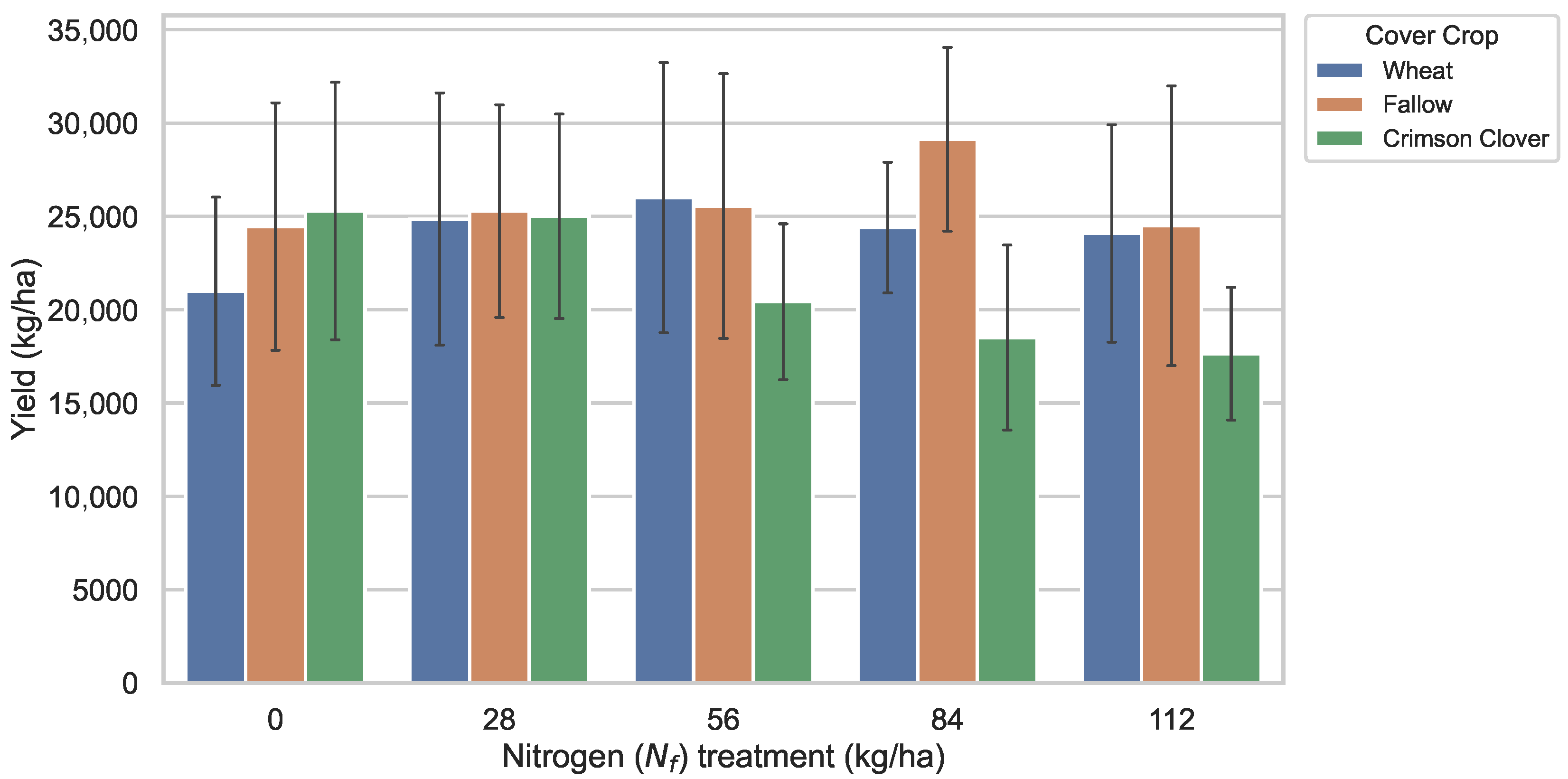
To further evaluate, we complemented the average bar plot illustrating sweet potato yield responses to $N_f$ and cover crop systems (Figure 5) with a two-way analysis of variance (ANOVA) assessing the interaction effects of $N_f$ and cover crop type. The ANOVA results (tabulated in

Table 3. Two-way ANOVA for nitrogen rate and cover crop effects on sweet potato yield. df = degrees of freedom; SS = sum of squares; MS = mean square (SS/df); F = F-statistic; p-value = significance level.

Source	df	SS	MS	F	p-Value
Nitrogen ($N_f$)	4	1.12$\times {10}^8$	2.79$\times {10}^7$	0.824	0.513
Cover Crop	2	3.96$\times {10}^8$	1.98$\times {10}^8$	5.83	0.00397 **
$N_f$ × Cover Crop	8	5.32$\times {10}^8$	6.64$\times {10}^7$	1.96	0.0588 †
Residual	105	3.56$\times {10}^9$	3.39$\times {10}^7$	—	—

** Significant at $p<0.01$. ^† Marginal effect ($0.05<p<0.10$).

) showed that nitrogen rate did not significantly influence yield ($p=0.513$), indicating that increasing $N_f$ from 0 to 112 kg/ha did not produce statistically meaningful changes in marketable storage root yield. In contrast, cover crop treatment had a significant effect on yield with $p=0.00397$, demonstrating that differences among fallow, wheat, and crimson clover systems contributed more to yield variation compared to $N_f$. The $N_f$ × cover crop interaction was found marginal ($p=0.0588$) but not statistically significant, suggesting that while some visual differences in nitrogen responsiveness were apparent across cover crops, these trends did not meet the threshold for statistical significance.

These statistical findings align closely with the agronomic yield patterns observed in Figure 4 and Figure 5. At low $N_f$ (0–28 kg/ha), crimson clover performed comparably to or slightly better than wheat and fallow, likely due to biological nitrogen supporting early crop development. At moderate-to-high $N_f$ (i.e., 56–84 kg/ha), fallow cover crop markedly outperformed wheat and crimson clover, demonstrating that in nutrient-rich environments, combining with cover crops may not confer yield benefits and can even hinder performance due to residue-driven nutrient immobilization. At the highest $N_f$ level (112 kg/ha), yield reductions were evident across all cover crops, with the steepest decline under crimson clover, reinforcing the negative impact of nutrient oversupply on tuber bulking. Overall, the barplot (Figure 5) reflects yield ranking patterns of fallow > wheat > crimson clover at high $N_f$, and crimson clover ≥ wheat ≥ fallow at low $N_f$. Such interaction patterns have been widely reported in cover-crop-based systems where legumes enhance productivity at low $N_f$ input, whereas non-legumes and fallow systems dominate under high-input intensification [55]. The ANOVA results confirm that these differences in cover crops are statistically meaningful. In contrast, the effects of $N_f$ and the $N_f$ × cover crop interaction were comparatively weaker, indicating that cover crop choice exerted a more consistent influence on sweet potato yield than nitrogen fertilization within the range tested.

5.3. Physiological Basis for Robust Feature Migration in Cross-Crop Transfer Learning

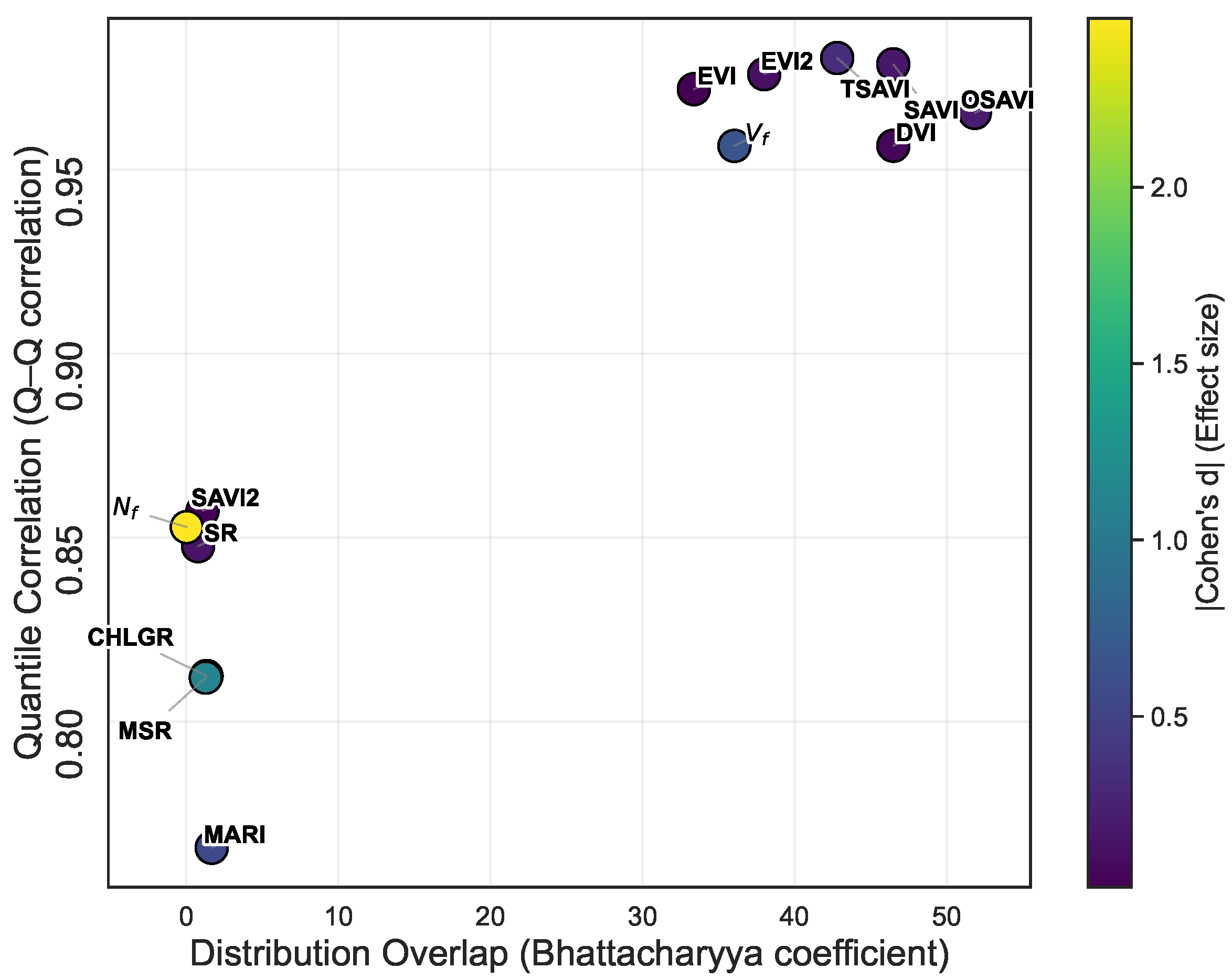
To quantitatively assess the robustness of the 13-selected features for cross-crop migration from potato (source domain) to sweet potato (target domain), we conducted a statistical comparison of each feature’s distributional behavior across the two datasets. Four complementary metrics were computed for each feature: (1) the Bhattacharyya coefficient (BC) as a measure of distributional overlap [56], (2) the Wasserstein distance to quantify absolute distributional shift [57], (3) Cohen’s |d| value to evaluate standardized effect size [58], and (4) quantile–quantile (Q–Q) correlation (r) [59], reflecting similarity in distributional shape after sample-size sorting.

The results illustrated in Figure 6 show that several features exhibit strong cross-crop robustness, characterized by substantial distributional overlap (BC ≥ 30), small standardized effect sizes (|d| < 0.2), minimal distributional shift (low Wasserstein distance), and very high quantile–quantile correlation (r ≥ 0.95). The most transferable features were EVI (BC = 33.37, |d| = 0.016, r = 0.972), EVI2 (BC = 38.00, |d| = 0.121, r = 0.976), SAVI (BC = 46.48, |d| = 0.168, r = 0.979), DVI (BC = 46.49, |d| = 0.064, r = 0.956), OSAVI (BC = 51.85, |d| = 0.205, r = 0.965), TSAVI (BC = 42.80, |d| = 0.325, r = 0.980), and the spatial canopy cover metric ($V_f$) (BC = 36.04, |d| = 0.662, r = 0.956). Physiologically, these predictors represent fundamental and conserved processes across broadleaf crops, including photosynthetic capacity, canopy development, and vegetation–soil interactions. Their stable cross-crop behavior explains why they remain highly predictive when transferred to a new species in a deep learning context.

Indices such as EVI, EVI2, DVI, SAVI, TSAVI, and OSAVI quantify generalized canopy vigor, greenness, and biomass accumulation, traits governed by core physiological processes including chlorophyll absorption, nitrogen assimilation, and leaf area expansion [20,60,61]. Because universal biochemical and biophysical pathways drive these mechanisms, the corresponding spectral indices exhibit similar spectral dynamics in both potato and sweet potato, resulting in high distributional similarity and minimal differences in effect sizes. Their robustness is further reinforced by their insensitivity to soil background, especially during mid-season canopy closure, which reduces species-specific artifacts. In contrast, indices designed for pigment-related behaviors, such as MARI (BC = 1.675, |d| = 0.567, r = 0.766), CHLGR (BC = 1.338, |d| = 0.474, r = 0.812), SR (BC = 0.777, |d| = 1.140, r = 0.848), and MSR (BC = 1.282, |d| = 1.132, r = 0.812), exhibited lower robustness. These indices are more sensitive to species-specific differences in leaf biochemistry, anatomical structure, and optical scattering properties. Because potato and sweet potato differ in leaf morphology, canopy layering, and chlorophyll density, these pigment-enhanced or nonlinear ratio indices displayed substantial distributional divergence across crops, reflected in very low BC-overlap (<2), large Wasserstein distances (≥3.6), and moderate-to-large effect sizes. These findings indicate that such features may introduce crop-specific bias when transferred directly without adaptation.

The spatial canopy descriptor ($V_f$) also emerged as a highly stable cross-crop metric. As an integrated structural indicator reflecting fractional vegetation cover, $V_f$ captures canopy geometry, planting density, and biomass status attributes that evolve in similar trajectories across the tuber and bulking stages of the root crops during bulking and maturation. The high Q–Q correlation (r = 0.956) and moderate BC-overlap demonstrate that canopy structural development is more similar across crops than fine-scale spectral variations, making $V_f$ an effective feature for transfer learning. In contrast, the agronomic variable $N_f$ exhibited the lowest cross-crop compatibility (BC = 0.0376, |d| = 2.48), which is expected because field-level fertilization regimes and management structures differ substantially between crops, violating assumptions required for feature transfer. As an external management factor rather than a plant-inherent physiological trait, nitrogen rates are not expected to transfer reliably across domains. Nevertheless, $N_f$ was kept in the feature subsets to preserve the full physiological and agronomic context used during source-domain model training and to enable a fair, one-to-one architectural transfer between the source and target domains.

5.4. Deep Transfer Learning Model Performance

The predictive performance of the hybrid CNN–RNN–Attention framework for sweet potato yield forecasting, developed through transfer learning from potato datasets [20], was systematically evaluated and compared with three baseline architecture: a standalone CNN, a BiGRU, and a BiLSTM. All models were tested across five phenological stages (emergence, hilling, tuberization, bulking, and maturity) and six predictor subset sizes ranging from 3F to 13F (detailed in Section 4). All architectures operate on sequential inputs, each phenological stage represents a cumulative time window. For example, the tuberization stage uses observations from emergence through tuberization, and the bulking stage uses data from emergence through bulking. This setup enabled controlled evaluation of how adding physiological relevant information influenced model performance. Model performance was assessed using the $R^2$ and percentage RMSE (%), as summarized in

Table 4. Performance of the CNN model across growth stages and varying predictor subset sizes.

Growth Stages	3F		5F		7F		9F		11F		13F
	${\mathit{R}}^{\mathbf{2}}$	RMSE (%)	${\mathit{R}}^{\mathbf{2}}$	RMSE (%)	${\mathit{R}}^{\mathbf{2}}$	RMSE (%)	${\mathit{R}}^{\mathbf{2}}$	RMSE (%)	${\mathit{R}}^{\mathbf{2}}$	RMSE (%)	${\mathit{R}}^{\mathbf{2}}$	RMSE (%)
Emergence	0.37	21.60%	0.53	21.05%	0.61	19.57%	0.58	19.21%	0.61	19.40%	0.61	19.77%
Hilling	0.46	22.65%	0.44	21.91%	0.52	20.44%	0.50	20.74%	0.59	19.65%	0.58	20.94%
Tuberization	0.56	22.75%	0.49	22.85%	0.59	20.98%	0.58	22.79%	0.62	19.32%	0.58	21.00%
Bulking	0.36	23.94%	0.37	23.16%	0.61	19.66%	0.56	20.75%	0.53	21.34%	0.46	22.49%
Maturity	0.44	24.44%	0.44	23.31%	0.49	22.37%	0.49	21.26%	0.53	21.80%	0.42	22.41%

,

Table 5. Performance of the BiGRU model across growth stages and varying predictor subset sizes.

Growth Stages	3F		5F		7F		9F		11F		13F
	${\mathit{R}}^{\mathbf{2}}$	RMSE (%)	${\mathit{R}}^{\mathbf{2}}$	RMSE (%)	${\mathit{R}}^{\mathbf{2}}$	RMSE (%)	${\mathit{R}}^{\mathbf{2}}$	RMSE (%)	${\mathit{R}}^{\mathbf{2}}$	RMSE (%)	${\mathit{R}}^{\mathbf{2}}$	RMSE (%)
Emergence	0.42	21.15%	0.49	20.15%	0.53	19.93%	0.59	19.74%	0.59	19.76%	0.56	19.81%
Hilling	0.52	20.59%	0.45	21.28%	0.58	19.69%	0.58	19.05%	0.53	20.33%	0.64	19.80%
Tuberization	0.55	20.58%	0.56	20.05%	0.56	19.51%	0.61	19.15%	0.62	19.53%	0.56	19.70%
Bulking	0.42	21.85%	0.49	21.51%	0.49	21.56%	0.56	20.41%	0.56	20.25%	0.59	19.83%
Maturity	0.38	22.16%	0.49	21.46%	0.58	19.82%	0.52	20.75%	0.53	20.28%	0.58	20.69%

,

Table 6. Performance of the BiLSTM model across growth stages and varying predictor subset sizes.

Growth Stages	3F		5F		7F		9F		11F		13F
	${\mathit{R}}^{\mathbf{2}}$	RMSE (%)	${\mathit{R}}^{\mathbf{2}}$	RMSE (%)	${\mathit{R}}^{\mathbf{2}}$	RMSE (%)	${\mathit{R}}^{\mathbf{2}}$	RMSE (%)	${\mathit{R}}^{\mathbf{2}}$	RMSE (%)	${\mathit{R}}^{\mathbf{2}}$	RMSE (%)
Emergence	0.41	21.79%	0.52	19.74%	0.53	19.51%	0.52	19.58%	0.50	19.31%	0.49	19.75%
Hilling	0.50	20.24%	0.48	21.52%	0.56	19.76%	0.64	18.68%	0.62	18.75%	0.53	20.94%
Tuberization	0.59	20.35%	0.58	20.29%	0.58	20.52%	0.62	19.64%	0.62	19.56%	0.56	21.28%
Bulking	0.45	21.66%	0.49	21.90%	0.58	21.09%	0.49	20.80%	0.50	21.23%	0.58	19.80%
Maturity	0.46	22.04%	0.49	21.37%	0.52	21.11%	0.48	23.57%	0.59	20.46%	0.58	20.01%

and

Table 7. Performance of the Hybrid CNN–RNN–Attention model across growth stages and varying predictor subset sizes.

Growth Stages	3F		5F		7F		9F		11F		13F
	${\mathit{R}}^{\mathbf{2}}$	RMSE (%)	${\mathit{R}}^{\mathbf{2}}$	RMSE (%)	${\mathit{R}}^{\mathbf{2}}$	RMSE (%)	${\mathit{R}}^{\mathbf{2}}$	RMSE (%)	${\mathit{R}}^{\mathbf{2}}$	RMSE (%)	${\mathit{R}}^{\mathbf{2}}$	RMSE (%)
Emergence	0.38	20.70%	0.46	20.42%	0.49	20.22%	0.52	20.17%	0.44	21.30%	0.37	21.87%
Hilling	0.55	20.10%	0.53	20.28%	0.61	18.91%	0.56	20.33%	0.55	20.98%	0.52	20.42%
Tuberization	0.56	19.61%	0.59	19.31%	0.64	18.18%	0.62	19.31%	0.59	19.45%	0.52	20.17%
Bulking	0.58	19.57%	0.66	18.03%	0.58	19.55%	0.52	19.86%	0.52	20.28%	0.49	20.84%
Maturity	0.49	21.08%	0.53	20.76%	0.61	18.66%	0.49	20.56%	0.53	20.97%	0.53	21.00%

, which together provide complementary perspectives on predictive accuracy and reliability.

At lower predictor subset sizes (3F–7F), the baseline recurrent models (BiGRU and BiLSTM) consistently outperformed the CNN baseline in terms of error minimization (Table 4, Table 5 and Table 6). For instance, at the emergence stage, CNN produced relatively high errors (RMSE = 21.60% at 3F; Table 4), whereas BiGRU and BiLSTM achieved modest improvements (21.15% and 21.79%, respectively; Table 5 and Table 6). More pronounced differences were observed during hilling, where CNN remained unstable with RMSE values exceeding 22% (Table 4), while BiGRU (20.59%; Table 5) and BiLSTM (20.24%; Table 5) demonstrated clear improvements. During tuberization, BiGRU and BiLSTM both achieved RMSE values of around 20%, whereas CNN required more features to achieve similar accuracy. These results highlight the superior capacity of recurrent architectures to leverage limited feature inputs through their inherent ability to capture sequential and temporal dependencies.

At higher predictor subset sizes (9F–13F), the divergence between models became more apparent. CNN exhibited increasing sensitivity to redundancy, with RMSE values deteriorating at later stages. For example, during bulking, CNN performance declined from an optimal 19.66% (7F) to 22.49% (13F) (Table 4), suggesting that additional features introduced noise rather than improving predictive power. In contrast, BiGRU displayed stability across higher dimensions, maintaining RMSE values consistently around 19.8–20.3% (Table 5). BiLSTM was the most resilient to redundancy, achieving superior performance at critical stages such as hilling ($R^2=0.64$ and RMSE = 18.68% at 9F) and Maturity ($R^2=0.58$ and RMSE = 20.01% at 13F) (Table 6). These outcomes underscore the advantage of recurrent models in filtering out irrelevant or redundant signals, thereby sustaining predictive reliability when feature dimensionality expands.

Against this backdrop, the hybrid CNN–RNN–Attention model (Table 7) consistently delivered superior performance. The model’s integration of convolutional filters for local feature extraction, recurrent layers for modeling short- and long-term dependencies, and an attention mechanism for adaptive weighting enabled it to capture physiologically relevant signals more effectively than any baseline. At tuberization, the hybrid model achieved its best results, with $R^2$ = 0.64 and RMSE = 18.18%, using seven robust predictors, yielding the highest correlation and a 1–4% reduction in RMSE relative to BiLSTM (19.64%) and BiGRU (19.15%). Similarly, during Bulking, the hybrid approach outperformed all baselines, peaking at $R^2$ = 0.66 and RMSE = 18.03% utilizing five robust predictors, whereas the best baseline (BiGRU) remained above 20%. These reductions in RMSE are particularly noteworthy given that they occurred at physiologically critical stages, where accurate yield prediction is most valuable. Even at later growth stages, when baseline models exhibited either performance plateaus (BiGRU, BiLSTM) or deterioration (CNN), the hybrid model maintained relatively low RMSE values. For example, at maturity, it achieved higher accuracy with $R^2$ = 0.61 and RMSE = 18.66% at 7F, outperforming CNN and RNN base models. Although performance gains were less pronounced at the emergence stage, the hybrid model still achieved stable improvements over CNN, particularly with smaller feature subsets. Overall, the hybrid model not only minimized error more effectively than the baselines but also demonstrated resilience to feature redundancy, achieving peak performance with intermediate subsets (5F and 7F) and avoiding the instability observed in CNN at higher dimensions.

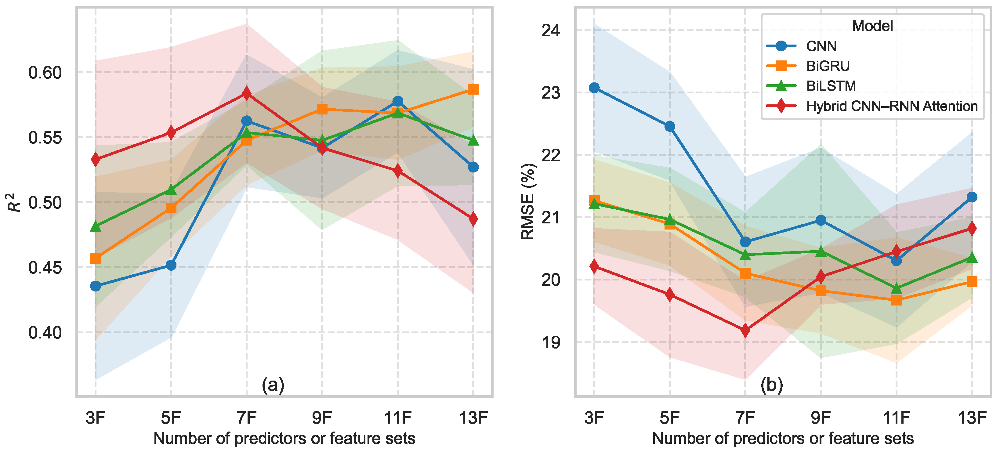
To complement the tabulated performance metrics (Table 4, Table 5, Table 6 and Table 7), Figure 7 provides a visual summary of model behavior across increasing feature subsets from 3F to 13F, where $R^2$ and percentage RMSE values were averaged across all growth stages. The hybrid architecture consistently achieved the higher $R^2$ and the lowest percentage RMSE values when using compact feature sets (3F–7F), demonstrating its efficiency in extracting meaningful representations without reliance on a large number of predictors. In particular, the hybrid deep transfer learning architecture achieved peak accuracy at 7F ($R^2\approx 0.64$, RMSE ≈ 18–19%). Whereas CNN, BiGRU, and BiLSTM required larger feature sets (11F–13F) to achieve similar performance. At higher feature dimensions, the baseline models showed moderate gains or plateauing, while the hybrid showed a decline, reflecting its sensitivity to redundant or noisy predictors. These findings suggest that the hybrid model delivers parsimonious learning by leveraging attention mechanisms to emphasize the most informative temporal-spectral cues, whereas baseline CNN and RNN architectures rely more on feature expansion. Significantly, this efficiency reduces computational cost, mitigates overfitting risk, and enhances robustness in data-limited scenarios, underscoring the hybrid architecture’s superiority for yield modeling in feature-limited environments.

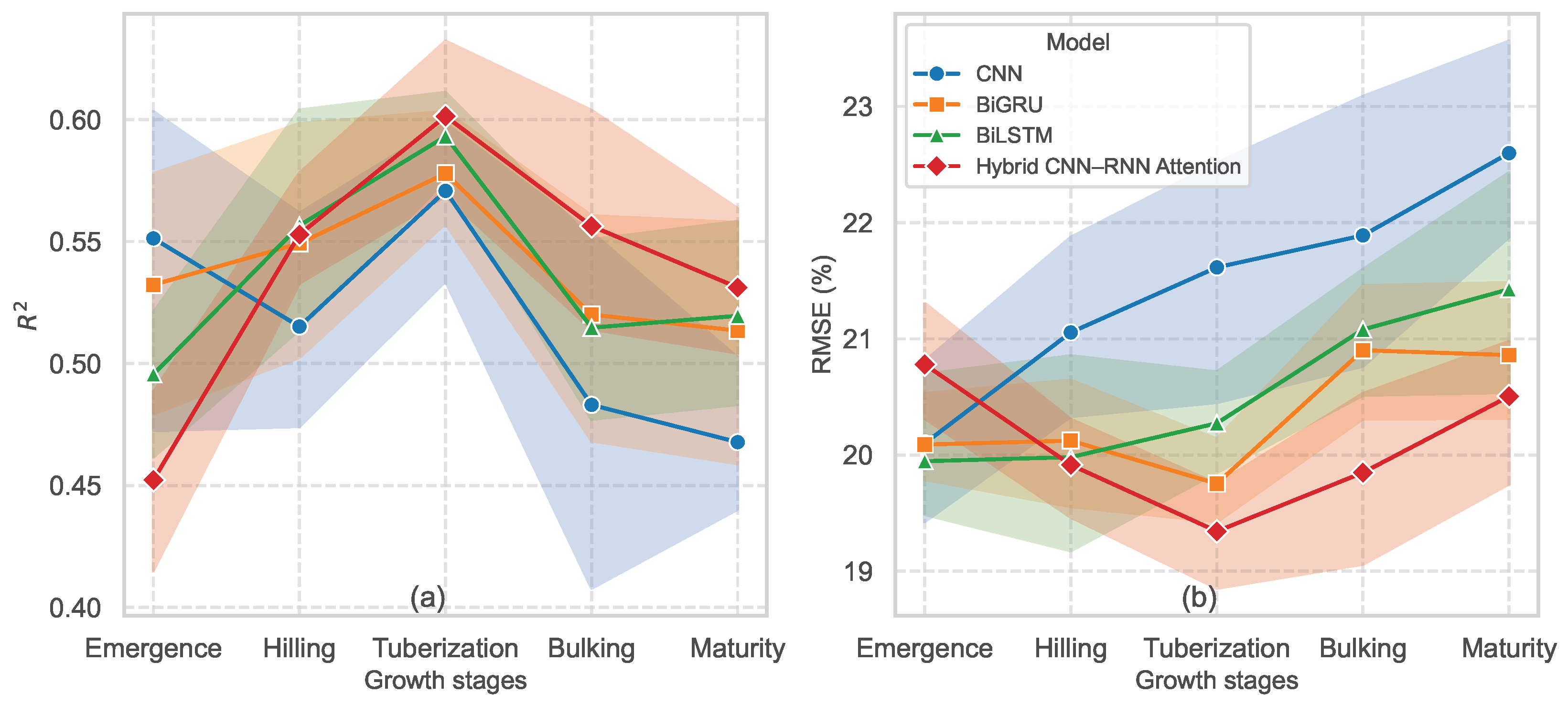
In addition, to further complement the tabulated performance metrics (Table 4, Table 5, Table 6 and Table 7), Figure 8 presents stage-wise trends, where performance metrics were averaged across all feature subset sizes (3F–13F) and compared across sweet potato growth stages. This visualization highlights temporal dependencies in model performance that are less apparent in feature-specific presentation. At the Emergence stage, the hybrid CNN–RNN–Attention underperformed relative to CNN, BiGRU, and BiLSTM. This reduced performance is likely due to sparse canopy cover and weak spectral contrast at early stages, when simpler recurrent models were better able to exploit the limited temporal signals, whereas the hybrid’s attention layers lacked sufficient informative cues to emphasize. However, from Hilling to Tuberization, performance improved substantially across all models, with tuberization marking the peak ($R^2\approx 0.62$, RMSE ≈ 19%). Here, the hybrid model achieved the most substantial gains, clearly outperforming CNN and recurrent baseline models. This superiority reflects its ability to integrate spectral–temporal features more effectively, capturing canopy closure and tuber initiation processes that are tightly linked to yield formation. At Bulking and Maturity, predictive accuracy declined for all models, consistent with spectral saturation and physiological senescence reducing vegetation index sensitivity. The CNN baseline exhibited the steepest deterioration (RMSE > 22%), while BiGRU and BiLSTM preserved moderate stability. The hybrid model also lost some of its advantage but remained the most robust overall, consistently achieving lower RMSE values than the baselines. This stage-specific peak also reflects the biological reality that canopy growth features up to tuberization maintain strong, monotonic relationships with underground storage-root development, whereas later-season data introduce spectral saturation, senescence-driven noise, and weakened canopy–yield coupling. As a result, adding sequential observations beyond tuberization contributes more noise than signal, reducing model accuracy despite access to longer time series.

5.5. Relevance of Feature Robustness in Model Performance

The performance patterns observed across the feature subsets (3F–13F) closely mirror the underlying robustness of the spectral and structural indices when transferred from potato to sweet potato. The base feature subset (3F) was intentionally designed to include one spectral index (SR), one spatial descriptor ($V_f$), and one agronomic factor ($N_f$), ensuring that the models started with a minimal but physiologically diverse representation of canopy vigor, structural development, and management inputs. Model performance at this stage was modest across all models (Refer Figure 7), reflecting the limited spectral information available. However, even at 3F, recurrent models (BiGRU and BiLSTM) outperformed CNN, demonstrating their inherent advantage in extracting temporal patterns from low-dimensional inputs.

Performance improved substantially when the first set of robust features (MARI and CHLGR) was added to the 5F subset. These features capture chlorophyll-related physiological processes that behave similarly across potato and sweet potato, as confirmed by their moderate distributional overlap and Q–Q correlations. All models benefited from this expansion, but the improvement was most pronounced for the hybrid CNN–RNN–Attention model, which leveraged both spectral-local and temporal-global cues to achieve the higher performance (Figure 7 and Figure 8). The most substantial gains occurred at the 7F subset, where OSAVI and SAVI2, two of the most statistically robust and physiologically transferable features, were introduced. Both indices demonstrate high BC overlap, low effect sizes, and very strong Q–Q alignment between crops. This corresponds directly to the peak performance observed across models at 7F, particularly for the hybrid model with $R^2\approx 0.64$ and RMSE ≈ 18%. Recurrent models also showed notable gains at 7F, but CNN exhibited instability, highlighting its sensitivity to variations in spectral distributions when domain-shift remains unresolved.

When additional features were introduced at 9F, 11F, and 13F (specifically MSR, TSAVI, SAVI, EVI, EVI2, and DVI), the marginal benefits became inconsistent across architectures. Although many of these indices are robust, their inclusion increased feature dimensionality and redundancy. Recurrent models (BiGRU and BiLSTM) maintained stability and often reached performance peaks (e.g., BiLSTM at 11F, Figure 7), owing to their ability to filter noisy or redundant inputs through gated recurrence. In contrast, CNN performance deteriorated at larger feature sets. The hybrid CNN–RNN–Attention architecture achieved its highest accuracy at moderate dimensionality (5F–7F) and subsequently declined as additional predictors were added. This behavior reflects the hybrid model’s sensitivity to redundant spectral inputs, which reduces the effectiveness of attention mechanisms that rely on distinct, informative cues. Compact feature subsets enriched with cross-crop-stable predictors (SAVI, OSAVI, EVI, EVI2, DVI, TSAVI, $V_f$) support efficient and accurate transfer learning across all architectures, with the hybrid model benefiting the most. In contrast, increasing feature dimensionality, even with physiologically meaningful indices, can introduce redundancy and exacerbate subtle distributional mismatches, particularly for CNN-based architectures. Recurrent models remain more resilient to feature inflation, but still exhibit diminishing returns beyond 7F.

6. Conclusions

This study highlights the importance of sweet potato yield optimization through combined management of nitrogen fertilization and cover crop strategy. Across two growing seasons, sweet potato yield responses showed that cover crop choice exerted a stronger and more consistent influence on productivity than nitrogen rate within the tested range. Fallow cover crop generally produced the highest yields at intermediate-to-high nitrogen inputs (56–84 kg/ha). In contrast, crimson clover conferred advantages at low nitrogen inputs (<56 kg/ha), while wheat exhibited intermediate performance. Two-way ANOVA confirmed that cover crop treatment exerted a statistically significant effect on sweet potato yield, whereas $N_f$ and the $N_f$ × cover crop interaction were not significant. This result indicates that synchrony between residue-derived nitrogen release and crop demand plays a more critical role in determining yield than increasing fertilizer inputs alone.

The cross-crop feature robustness analysis demonstrated that vegetation indices capturing general canopy vigor, structural development, and soil–vegetation contrast (EVI, EVI2, DVI, SAVI, OSAVI, TSAVI, and $V_f$) exhibit high distributional similarity between potato and sweet potato. Conversely, pigment-enhanced indices such as MARI, CHLGR, SR, MSR, and the agronomic factor ($N_f$) showed poor transferability due to species-specific differences in leaf biochemistry and management-driven variability. This robustness pattern was reflected in model behavior. All deep learning architectures improved markedly when compact feature subsets were enriched with robust indices, particularly at 5F and 7F. However, further expansion to 9F–13F yielded marginal gain (or even reduced accuracy), due to increased feature dimensionality and redundancy.

Among the evaluated models, the hybrid CNN–RNN–Attention architecture consistently delivered the highest accuracy and lowest RMSE, particularly incorporating physiologically critical stages. After incorporating cumulative spectral–temporal inputs up to tuberization, the model achieved $R^2=0.64$ and RMSE = 18.18%, outperforming the CNN (RMSE = 20.98%), BiGRU (19.51%), and BiLSTM (20.52%) while using only seven robust predictors. Likewise, after incorporating data through the bulking stage, the hybrid model reached $R^2=0.66$ and RMSE = 18.03%, whereas the best recurrent baseline (BiGRU) remained above 20%. Collectively, these findings highlight that (i) agronomic context, especially cover crop selection, strongly conditions yield outcomes, and (ii) integrating robustness-aware feature design with hybrid deep transfer learning enables reliable cross-crop yield prediction from limited, physiologically meaningful input features.

Although the proposed transfer learning framework produced strong results, several limitations remain. The model was evaluated only under humid subtropical conditions in Pontotoc County, Mississippi and on a single sweet potato variety, leaving its robustness across contrasting climates and cultivars untested. Management-driven domain shifts, such as fertilization regimes, residue management, and planting geometry, may also limit broader generalization. Future work should evaluate cross-climate and multi-variety performance, incorporate adaptive or sparsity-aware feature selection to reduce redundancy, and develop stage-agnostic or continuous-time models. Integrating transformer-based architectures to capture long-range temporal dependencies and expanding validation to other root and tuber crops will further strengthen physiological scalability across diverse agroecological systems.

References

1. Goodfellow, I.; Bengio, Y.; Courville, A.; Bengio, Y. Deep Learning; MIT Press: Hoboken, NJ, USA, 2016; Volume 1. [Google Scholar]
2. Ma, Y.; Chen, S.; Ermon, S.; Lobell, D.B. Transfer learning in environmental remote sensing. Remote Sens. Environ. 2024, 301, 113924. [Google Scholar] [CrossRef]
3. Xu, J.; Zhu, Y.; Zhong, R.; Lin, Z.; Xu, J.; Jiang, H.; Huang, J.; Li, H.; Lin, T. DeepCropMapping: A multi-temporal deep learning approach with improved spatial generalizability for dynamic corn and soybean mapping. Remote Sens. Environ. 2020, 247, 111946. [Google Scholar] [CrossRef]
4. Gadiraju, K.K.; Vatsavai, R.R. Remote sensing based crop type classification via deep transfer learning. IEEE J. Sel. Top. Appl. Earth Obs. Remote Sens. 2023, 16, 4699–4712. [Google Scholar] [CrossRef]
5. Joshi, A.; Pradhan, B.; Chakraborty, S.; Varatharajoo, R.; Gite, S.; Alamri, A. Deep-Transfer-Learning Strategies for Crop Yield Prediction Using Climate Records and Satellite Image Time-Series Data. Remote Sens. 2024, 16, 4804. [Google Scholar] [CrossRef]
6. Wang, A.X.; Tran, C.; Desai, N.; Lobell, D.; Ermon, S. Deep transfer learning for crop yield prediction with remote sensing data. In Proceedings of the 1st ACM SIGCAS Conference on Computing and Sustainable Societies, Menlo Park and San Jose, CA, USA, 20–22 June 2018; pp. 1–5. [Google Scholar]
7. Ma, Y.; Zhang, Z.; Yang, H.L.; Yang, Z. An adaptive adversarial domain adaptation approach for corn yield prediction. Comput. Electron. Agric. 2021, 187, 106314. [Google Scholar] [CrossRef]
8. Li, J.; Zhao, X.; Xu, H.; Zhang, L.; Xie, B.; Yan, J.; Zhang, L.; Fan, D.; Li, L. An interpretable high-accuracy method for rice disease detection based on multisource data and transfer learning. Plants 2023, 12, 3273. [Google Scholar] [CrossRef] [PubMed]
9. Hossen, M.I.; Awrangjeb, M.; Pan, S.; Mamun, A.A. Transfer learning in agriculture: A review. Artif. Intell. Rev. 2025, 58, 97. [Google Scholar] [CrossRef]
10. Canton, H. Food and agriculture organization of the United Nations-FAO. In The Europa Directory of International Organizations 2021; Routledge: London, UK, 2021; pp. 297–305. [Google Scholar]
11. Qin, Y.; Naumovski, N.; Ranadheera, C.S.; D’Cunha, N.M. Nutrition-related health outcomes of sweet potato (Ipomoea batatas) consumption: A systematic review. Food Biosci. 2022, 50, 102208. [Google Scholar] [CrossRef]
12. Food and Agriculture Organization of the United Nations. World Food and Agriculture Statistical Yearbook 2020; Food and Agriculture Organization of the United Nations: Rome, Italy, 2020. [Google Scholar]
13. Weber, C.; Hevesh, A.; Davis, W.V. US Sweet Potatoes Are Enjoyed Around the World, Export Data Show. 2023. Available online: https://www.ers.usda.gov/data-products/charts-of-note/chart-detail?chartId=105095 (accessed on 5 August 2025).
14. George, J.; Reddy, G.V.; Wadl, P.A.; Rutter, W.; Culbreath, J.; Lau, P.W.; Rashid, T.; Allan, M.C.; Johaningsmeier, S.D.; Nelson, A.M.; et al. Sustainable sweet potato Production in the United States: Current Status, Challenges, and Opportunities. Agron. J. 2024, 116, 630–660. [Google Scholar] [CrossRef]
15. Araus, J.L.; Cairns, J.E. Field high-throughput phenotyping: The new crop breeding frontier. Trends Plant Sci. 2014, 19, 52–61. [Google Scholar] [CrossRef]
16. Farella, A.; Paciolla, F.; Quartarella, T.; Pascuzzi, S. Agricultural unmanned ground vehicle (UGV): A brief overview. In International Symposium on Farm Machinery and Processes Management in Sustainable Agriculture; Springer Nature: Cham, Switzerland, 2024; pp. 137–146. [Google Scholar]
17. Agelli, M.; Corona, N.; Maggio, F.; Moi, P. Unmanned ground vehicles for continuous crop monitoring in agriculture: Assessing the readiness of current ICT technology. Machines 2024, 12, 750. [Google Scholar] [CrossRef]
18. De Castro, A.; Shi, Y.; Maja, J.; Peña, J. UAVs for vegetation monitoring: Overview and recent scientific contributions. Remote Sens. 2021, 13, 2139. [Google Scholar] [CrossRef]
19. Lungu, O.; Chabala, L.; Shepande, C. Satellite-based crop monitoring and yield estimation—A review. J. Agric. Sci. 2020, 13, 180. [Google Scholar] [CrossRef]
20. Yadav, S.A.; Zhang, X.; Wijewardane, N.K.; Feldman, M.; Qin, R.; Huang, Y.; Samiappan, S.; Young, W.; Tapia, F.G. Context-Aware Deep Learning Model for Yield Prediction in Potato Using Time-Series UAS Multispectral Data. IEEE J. Sel. Top. Appl. Earth Obs. Remote Sens. 2025, 18, 6096–6115. [Google Scholar] [CrossRef]
21. Wu, B.; Zhang, M.; Zeng, H.; Tian, F.; Potgieter, A.B.; Qin, X.; Yan, N.; Chang, S.; Zhao, Y.; Dong, Q.; et al. Challenges and opportunities in remote sensing-based crop monitoring: A review. Natl. Sci. Rev. 2023, 10, nwac290. [Google Scholar] [CrossRef]
22. Singh, K.; Huang, Y.; Young, W.; Harvey, L.; Hall, M.; Zhang, X.; Lobaton, E.; Jenkins, J.; Shankle, M. Sweet Potato Yield Prediction Using Machine Learning Based on Multispectral Images Acquired from a Small Unmanned Aerial Vehicle. Agriculture 2025, 15, 420. [Google Scholar] [CrossRef]
23. Tedesco, D.; de Almeida Moreira, B.R.; Júnior, M.R.B.; Papa, J.P.; da Silva, R.P. Predicting on multi-target regression for the yield of sweet potato by the market class of its roots upon vegetation indices. Comput. Electron. Agric. 2021, 191, 106544. [Google Scholar] [CrossRef]
24. Liu, H.; Hunt, S.; Yencho, G.C.; Pecota, K.V.; Mierop, R.; Williams, C.M.; Jones, D.S. Predicting sweet potato traits using machine learning: Impact of environmental and agronomic factors on shape and size. Comput. Electron. Agric. 2024, 225, 109215. [Google Scholar] [CrossRef]
25. Zhou, H.; Huang, F.; Lou, W.; Gu, Q.; Ye, Z.; Hu, H.; Zhang, X. Yield prediction through UAV-based multispectral imaging and deep learning in rice breeding trials. Agric. Syst. 2025, 223, 104214. [Google Scholar] [CrossRef]
26. Kumar, C.; Dhillon, J.; Huang, Y.; Reddy, K. Explainable machine learning models for corn yield prediction using UAV multispectral data. Comput. Electron. Agric. 2025, 231, 109990. [Google Scholar] [CrossRef]
27. Wang, Y.; Zhang, Q.; Yu, F.; Zhang, N.; Li, Y.; Wang, M.; Zhang, J. Progress in Research on Deep Learning-Based Crop Yield Prediction. Agronomy 2024, 14, 2264. [Google Scholar] [CrossRef]
28. Sweet, D.D.; Tirado, S.B.; Springer, N.M.; Hirsch, C.N.; Hirsch, C.D. Opportunities and challenges in phenotyping row crops using drone-based RGB imaging. Plant Phenome J. 2022, 5, e20044. [Google Scholar] [CrossRef]
29. Long, J.; Liu, T.; Woznicki, S.A.; Marković, M.; Marko, O.; Sears, M. From Time-series Generation, Model Selection to Transfer Learning: A Comparative Review of Pixel-wise Approaches for Large-scale Crop Mapping. arXiv 2025, arXiv:2507.12590. [Google Scholar]
30. Chen, J.M. Evaluation of vegetation indices and a modified simple ratio for boreal applications. Can. J. Remote Sens. 1996, 22, 229–242. [Google Scholar] [CrossRef]
31. Gitelson, A.A.; Chivkunova, O.B.; Merzlyak, M.N. Nondestructive estimation of anthocyanins and chlorophylls in anthocyanic leaves. Am. J. Bot. 2009, 96, 1861–1868. [Google Scholar] [CrossRef]
32. Gitelson, A.A.; Viña, A.; Ciganda, V.; Rundquist, D.C.; Arkebauer, T.J. Remote estimation of canopy chlorophyll content in crops. Geophys. Res. Lett. 2005, 32. [Google Scholar] [CrossRef]
33. Rondeaux, G.; Steven, M.; Baret, F. Optimization of soil-adjusted vegetation indices. Remote Sens. Environ. 1996, 55, 95–107. [Google Scholar] [CrossRef]
34. Major, D.; Baret, F.; Guyot, G. A ratio vegetation index adjusted for soil brightness. Int. J. Remote Sens. 1990, 11, 727–740. [Google Scholar] [CrossRef]
35. Baret, F.; Guyot, G. Potentials and limits of vegetation indices for LAI and APAR assessment. Remote Sens. Environ. 1991, 35, 161–173. [Google Scholar] [CrossRef]
36. Huete, A.; Didan, K.; Miura, T.; Rodriguez, E.P.; Gao, X.; Ferreira, L.G. Overview of the radiometric and biophysical performance of the MODIS vegetation indices. Remote Sens. Environ. 2002, 83, 195–213. [Google Scholar]
37. Jordan, C.F. Derivation of leaf-area index from quality of light on the forest floor. Ecology 1969, 50, 663–666. [Google Scholar]
38. Pan, S.J.; Yang, Q. A survey on transfer learning. IEEE Trans. Knowl. Data Eng. 2009, 22, 1345–1359. [Google Scholar] [CrossRef]
39. Huber, F.; Inderka, A.; Steinhage, V. Leveraging remote sensing data for yield prediction with deep transfer learning. Sensors 2024, 24, 770. [Google Scholar] [CrossRef] [PubMed]
40. Chen, J.; Chen, J.; Zhang, D.; Sun, Y.; Nanehkaran, Y.A. Using deep transfer learning for image-based plant disease identification. Comput. Electron. Agric. 2020, 173, 105393. [Google Scholar] [CrossRef]
41. Coulibaly, S.; Kamsu-Foguem, B.; Kamissoko, D.; Traore, D. Deep neural networks with transfer learning in millet crop images. Comput. Ind. 2019, 108, 115–120. [Google Scholar] [CrossRef]
42. Khaki, S.; Pham, H.; Wang, L. Simultaneous corn and soybean yield prediction from remote sensing data using deep transfer learning. Sci. Rep. 2021, 11, 11132. [Google Scholar] [CrossRef]
43. Ketkar, N.; Moolayil, J. Convolutional neural networks. In Deep Learning with Python: Learn Best Practices of Deep Learning Models with PyTorch; Apress: Berkeley, CA, USA, 2021; pp. 197–242. [Google Scholar]
44. Schuster, M.; Paliwal, K.K. Bidirectional recurrent neural networks. IEEE Trans. Signal Process. 1997, 45, 2673–2681. [Google Scholar] [CrossRef]
45. Vaswani, A.; Shazeer, N.; Parmar, N.; Uszkoreit, J.; Jones, L.; Gomez, A.N.; Kaiser, Ł.; Polosukhin, I. Attention is all you need. Adv. Neural Inf. Process. Syst. 2017, 30. [Google Scholar]
46. Nejad, S.M.M.; Abbasi-Moghadam, D.; Sharifi, A.; Farmonov, N.; Amankulova, K.; Lászlź, M. Multispectral crop yield prediction using 3D-convolutional neural networks and attention convolutional LSTM approaches. IEEE J. Sel. Top. Appl. Earth Obs. Remote Sens. 2022, 16, 254–266. [Google Scholar]
47. Bergstra, J.; Bengio, Y. Random search for hyper-parameter optimization. J. Mach. Learn. Res. 2012, 13, 281–305. [Google Scholar]
48. Villordon, A.Q.; La Bonte, D.R.; Firon, N.; Kfir, Y.; Pressman, E.; Schwartz, A. Characterization of adventitious root development in sweet potato. HortScience 2009, 44, 651–655. [Google Scholar] [CrossRef]
49. Villordon, A.; Solis, J.; LaBonte, D.; Clark, C. Development of a prototype Bayesian network model representing the relationship between fresh market yield and some agroclimatic variables known to influence storage root initiation in sweet potato. HortScience 2010, 45, 1167–1177. [Google Scholar]
50. Larkin, R.P.; Griffin, T.S.; Honeycutt, C.W. Rotation and cover crop effects on soilborne potato diseases, tuber yield, and soil microbial communities. Plant Dis. 2010, 94, 1491–1502. [Google Scholar] [CrossRef] [PubMed]
51. Duan, W.; Zhang, H.; Xie, B.; Wang, B.; Zhang, L. Impacts of nitrogen fertilization rate on the root yield, starch yield and starch physicochemical properties of the sweet potato cultivar Jishu 25. PLoS ONE 2019, 14, e0221351. [Google Scholar] [CrossRef] [PubMed]
52. Crews, T.E.; Peoples, M. Legume versus fertilizer sources of nitrogen: Ecological tradeoffs and human needs. Agric. Ecosyst. Environ. 2004, 102, 279–297. [Google Scholar] [CrossRef]
53. Bakht, J.; Shafi, M.; Jan, M.T.; Shah, Z. Influence of crop residue management, cropping system and N fertilizer on soil N and C dynamics and sustainable wheat (Triticum aestivum L.) production. Soil Tillage Res. 2009, 104, 233–240. [Google Scholar] [CrossRef]
54. Ravi, V.; Chakrabarti, S.; Makeshkumar, T.; Saravanan, R. Molecular regulation of storage root formation and development in sweet potato. Hortic. Rev. 2014, 42, 157–208. [Google Scholar]
55. Dabney, S.M.; Delgado, J.A.; Meisinger, J.J.; Schomberg, H.H.; Liebig, M.A.; Kaspar, T.; Mitchell, J.; Reeves, W. Using cover crops and cropping systems for nitrogen management. Adv. Nitrogen Manag. Water Qual. 2010, 66, 231–282. [Google Scholar]
56. Bhattacharyya, A. On a measure of divergence between two statistical populations defined by their probability distribution. Bull. Calcutta Math. Soc. 1943, 35, 99–110. [Google Scholar]
57. Peyré, G.; Cuturi, M. Computational optimal transport: With applications to data science. Found. Trends® Mach. Learn. 2019, 11, 355–607. [Google Scholar] [CrossRef]
58. Cohen, J. Statistical Power Analysis for the Behavioral Sciences; Routledge: New York, NY, USA, 2013. [Google Scholar]
59. Wilk, M.B.; Gnanadesikan, R. Probability plotting methods for the analysis for the analysis of data. Biometrika 1968, 55, 1–17. [Google Scholar] [CrossRef] [PubMed]
60. Clevers, J.G.; Kooistra, L.; Van den Brande, M.M. Using Sentinel-2 data for retrieving LAI and leaf and canopy chlorophyll content of a potato crop. Remote Sens. 2017, 9, 405. [Google Scholar] [CrossRef]
61. Binte Mostafiz, R.; Noguchi, R.; Ahamed, T. Agricultural land suitability assessment using satellite Remote Sensing-derived soil-vegetation indices. Land 2021, 10, 223. [Google Scholar] [CrossRef]
Figure 1. Geographic location and experimental field layout at the Pontotoc Ridge–Flatwoods Branch Experiment Station, Mississippi State University. (a) Map of Mississippi highlighting the study region Pontotoc county. (b) High-resolution Google Satellite imagery highlighting the experimental field (outlined in red) within the surrounding landscape. (c) Detailed field design showing 60 experimental plots arranged in a randomized complete block design. Each plot represents a unique treatment combination of cover crop (Wheat, Fallow, or Crimson Clover) and nitrogen rate (N1: 0 kg/ha, N2: 28 kg/ha, N3: 56 kg/ha, N4: 84 kg/ha, N5: 112 kg/ha).
Remotesensing 17 04054 g001
Figure 2. Variable of importance in projection (VIP) based feature engineering utilizing PLSR algorithm on source domain datasets.
Remotesensing 17 04054 g002
Figure 3. Schematic representation of the proposed Hybrid CNN–RNN–Attention architecture with parameter-based transfer learning.
Remotesensing 17 04054 g003
Figure 4. Sweet potato yield (kg/ha) box plot variation under varying nitrogen ( N f ) treatments (0, 28, 56, 84, and 112 kg/ha) and cover crop management systems (Wheat, Fallow, and Crimson Clover) across two growing seasons: (a) 2022 and (b) 2023.
Remotesensing 17 04054 g004
Figure 5. Combined sweet potato yield bar plot along with standard deviation error bars under five nitrogen ( N f ) treatments (0, 28, 56, 84, and 112 kg/ha) across three cover crop systems (Wheat, Fallow, and Crimson Clover).
Remotesensing 17 04054 g005
Figure 6. Cross-Crop Spectral Robustness Map.
Remotesensing 17 04054 g006
Figure 7. Shared legend: Comparative performance of four deep transfer learning models, namely, CNN, BiGRU, BiLSTM, and the Hybrid CNN–RNN–Attention, across feature subsets (3F–13F). (a) R 2 and (b) percentage RMSE(%). Shaded regions represent confidence intervals.
Remotesensing 17 04054 g007
Figure 8. Shared legend: Stage-wise performance comparison of four deep learning architectures, namely, CNN, BiGRU, BiLSTM, and the proposed Hybrid CNN–RNN–Attention, across five critical potato growth stages. (a) R 2 and (b) percentage RMSE(%). Shaded regions denote confidence intervals.
Remotesensing 17 04054 g008