Article

Monitoring Rubber Plantation Distribution and Biomass with Sentinel-2 Using Deep Learning and Machine Learning Algorithm (2019–2024)


1
National Key Laboratory for Tropical Crop Breeding, School of Breeding and Multiplication (Sanya Institute of Breeding and Multiplication), Hainan University, Sanya 572025, China
2
Intelligent Forestry Key Laboratory of Haikou City, School of Tropical Agriculture and Forestry, Hainan University, Haikou 570228, China
3
School of Information and Communication Engineering, Hainan University, Haikou 570228, China
4
College of Geographical Sciences, Harbin Normal University, Harbin 150025, China
5
Department of Global Agricultural Sciences, Graduate School of Agricultural and Life Sciences, The University of Tokyo, Tokyo 113-8657, Japan
6
Faculty of Agriculture, King Michael I of Romania University of Life Sciences Timisoara, 119 Aradului Avenue, 300645 Timisoara, Romania
*
Author to whom correspondence should be addressed.
These authors contributed equally to this work.
Remote Sens. 2025, 17(24), 4042; https://doi.org/10.3390/rs17244042
Submission received: 31 October 2025 / Revised: 9 December 2025 / Accepted: 13 December 2025 / Published: 16 December 2025

Highlights

What are the main findings?
  • Rubber forests can be identified with high precision in Sentinel-2 remote sensing images by combining a multi-rule synthesized KNDVI index with a deep learning model.
  • The inclusion of structural parameters, such as canopy height and an enhanced vegetation index (EVI), improves the accuracy of biomass estimation.
What is the implication of the main finding?
  • The constructed multi-source data fusion and machine learning modeling framework is expected to have strong generalizability.
  • This study provides a technical approach for the precise monitoring of tropical rubber forests and the assessment of carbon storage.

Abstract
The number of rubber plantations has increased significantly since 2000, especially in Southeast Asia and China, and their ecological impacts are becoming more evident. A robust rubber supply monitoring system is currently required at both the production and ecological levels. This study used Sentinel-2 multi-rule remote sensing images and a deep learning method to construct a deep learning model that could generate a distribution map of rubber plantations in Danzhou City, Hainan Province, from 2019 to 2024. For biomass modeling, 52 sample plots (27 of which were historical plots) were integrated, and the canopy structure was extracted as an auxiliary variable from the point cloud data generated by an unmanned aerial vehicle survey. Five algorithms, namely Random Forest (RF), Gradient Boosting Decision Tree, Convolutional Neural Network, Back Propagation Neural Network, and Extreme Gradient Boosting, were used to characterize the spatiotemporal changes in rubber plantation biomass and analyze the driving mechanisms. The developed deep learning model was exceptional at identifying rubber plantations (overall accuracy = 91.63%, Kappa = 0.83). The RF model performed the best in terms of biomass prediction (R2 = 0.72, RRMSE = 21.48 Mg/ha). Research shows that canopy height as a characteristic factor enhances the explanatory power and stability of the biomass model. However, due to limitations such as sample plot size, image differences, canopy closure degree, and point cloud density, uncertainties in its generalization across years and regions remain. In summary, the proposed framework effectively captures the spatial and temporal dynamics of rubber plantations and estimates their biomass with high accuracy. This study provides a crucial reference for the refined management and ongoing monitoring of rubber plantations.

Graphical Abstract

1. Introduction

The rubber tree (Brazilian rubber tree) is an indispensable raw material used in the manufacturing of various products such as tires, medical devices, and defense equipment. It is primarily distributed in tropical and subtropical regions [1]. Specifically, Southeast Asia is the global center for rubber production, accounting for over 70% of its planting area, and China is also a major producer [2]. While the expansion of rubber plantations has supported market demand, it has also become an important driver of forest loss and ecological degradation, threatening biodiversity and carbon storage [3,4,5]. Since the 2000s, the expansion of rubber plantations has had increasingly severe ecological impacts. Consequently, there is an urgent need to establish strong monitoring methods at both the production and ecological levels to ensure sustainable practices and mitigate ecological effects [6]. After 2015, the rubber plantation area exhibited a significant downward trend, and its spatial distribution showed evident heterogeneity. Dense clusters of immature artificial forests characterized the western and northern regions of Hainan, while sparse clusters of artificial forests dominated the eastern coastal areas [7]. To help elucidate the effectiveness of the existing protection measures and the actual growth situation of rubber plantations, we must understand the dynamic changes in the rubber plantation area over time, the spatiotemporal evolution processes, and the response and adaptation mechanisms with respect to population growth, economic development, climate environment, and natural factors. When monitoring rubber plantations, on-site investigations are time-consuming and require a significant amount of manpower and resources. In contrast, remote sensing has also been utilized as an effective and timely monitoring method for rubber plantations [8,9].
The rapid advancement of remote sensing technologies has facilitated the improved identification of rubber plantations. With the increasing availability of medium spatial resolution remote sensing data, the method of capturing the phenological characteristics of rubber trees by combining Landsat time series images has become mainstream, reflecting its wide availability and historical archive [10]. The Sentinel-2 multispectral imaging satellite has a high spatial resolution (10 m) and five bands in the near-infrared spectral region, which provides a more accurate guarantee for the temporal monitoring of rubber plantation distributions [11]. Deep learning and machine learning methods employ reasoning and sample-based learning approaches in their classification algorithms to derive corresponding classification rules from a large dataset. They have excellent generalization capabilities and can effectively improve the accuracy of rubber plantation extraction, making them more suitable for handling large-scale datasets. Traditional machine learning algorithms, such as random forest [12,13,14] and support vector machine [15], have been increasingly used to map rubber plantations and have proven to be invaluable [16].
Accurate canopy height maps are crucial for accurately estimating the productivity, carbon storage, and biomass of rubber plantations. Traditional field surveys usually involve establishing sample plots and using lidar for highly accurate measurements. However, they are limited by the high cost, manpower requirements, and the limited measurement space [17,18]. In recent years, numerous researchers have addressed this issue using both active and passive remote sensing technologies. Although passive remote sensing technologies alleviate these challenges by providing high spatial and temporal resolution data, their effectiveness is affected by cloud cover and the inherent instability of measurement accuracy in complex terrain [19]. Active remote sensing technologies, especially LiDAR, use laser beams to scan the ground and collect three-dimensional data through the reflection signals obtained from the terrain, structure, and vegetation [20]. In contrast, space-based systems, such as the Ice, Cloud and Land Elevation Satellite (ICESat) and the Global Ecosystem Dynamics Investigation (GEDI), provide extensive coverage and fill the gap in near-surface remote sensing [21].
Aboveground biomass is a crucial indicator of forest growth and quality, playing a significant role in forest ecosystem monitoring, including the global carbon cycle, and assessing forest health. Rapid, accurate, and non-destructive assessments of the aboveground biomass in rubber plantations not only help predict rubber yields but also contribute to our understanding of carbon storage in tropical regions [22]. Traditional manual field measurements are one of the most commonly used methods for estimating aboveground biomass and have high accuracy. However, this method is time-consuming, labor-intensive, and is generally applied to small-scale areas. Compared with ground surveys, remote sensing technology has the advantages of being real-time, non-destructive, and applicable to large-scale areas, enabling more efficient and accurate estimation of forest aboveground biomass [23,24]. The establishment of a multi-source and multi-scale remote sensing estimation model for aboveground biomass in rubber plantations by integrating these two methods will undoubtedly enhance the accuracy of rubber plantation biomass estimation, thereby providing more scientific and reliable technical support, aiding in carbon storage assessments, and facilitating the elucidation of ecosystem service functions.
Although machine learning algorithms have been widely used in rubber plantations mapping research, their high dependence on sample size and representativeness limits their effectiveness in cases with insufficient samples; as a core indicator for forest carbon storage and ecosystem function studies, the precise estimation of biomass is highly dependent on the characterization of forest structural parameters, among which canopy height is regarded as the most critical determinant factor. Although biomass inversion methods based on canopy height have made significant progress, in large-scale and high-resolution scenarios, data saturation effects and insufficient estimation accuracy still constitute the main bottlenecks.
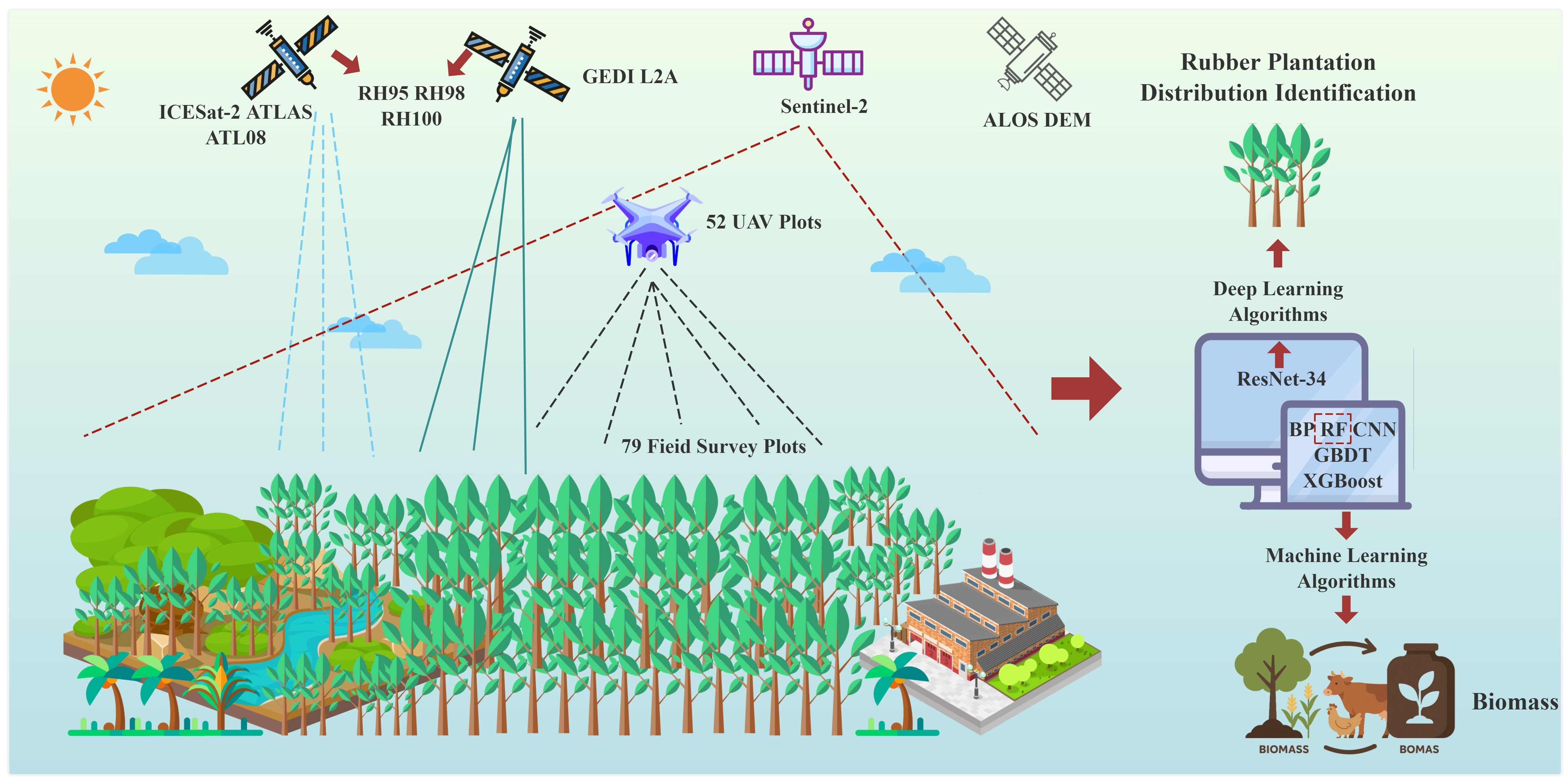
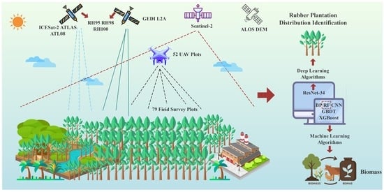
This study integrates multi-source remote sensing data and employs deep learning algorithms to conduct dynamic monitoring of rubber plantations in Danzhou City, Hainan Province. Based on machine learning algorithms such as Random Forest (RF), Backpropagation Neural Network (BP), Convolutional Neural Network (CNN), Gradient Boosting Decision Tree (GBDT), and Extreme Gradient Boosting (XGBoost), it also conducts dynamic monitoring of rubber biomass (see Figure 1 for the technical route). The main objectives include: (1) construct a trainingdeep learning model for multi-rule fusion, revealing the dynamic distribution patterns of rubber plantations in Danzhou City, Hainan Province from 2019 to 2024; (2) Combining two types of spaceborne LiDAR data (ICESat-2 and GEDI) to compensate for the limitations of a single data source in terms of spatial coverage and accuracy, thereby improving the estimation accuracy of canopy structural parameters and biomass inversion; (3) Selecting the most suitable biomass estimation model for this region by comparing different algorithms; (4) Drawing distribution maps of tree height and biomass density of rubber plantations in Danzhou City, Hainan Island from 2019 to 2024. This study provides innovative methods and technical support for the refined management of the rubber plantations ecosystem in Hainan Island. It is also of great significance for promoting the sustainable development of the natural rubber industry.

2. Materials and Methods

2.1. Study Area

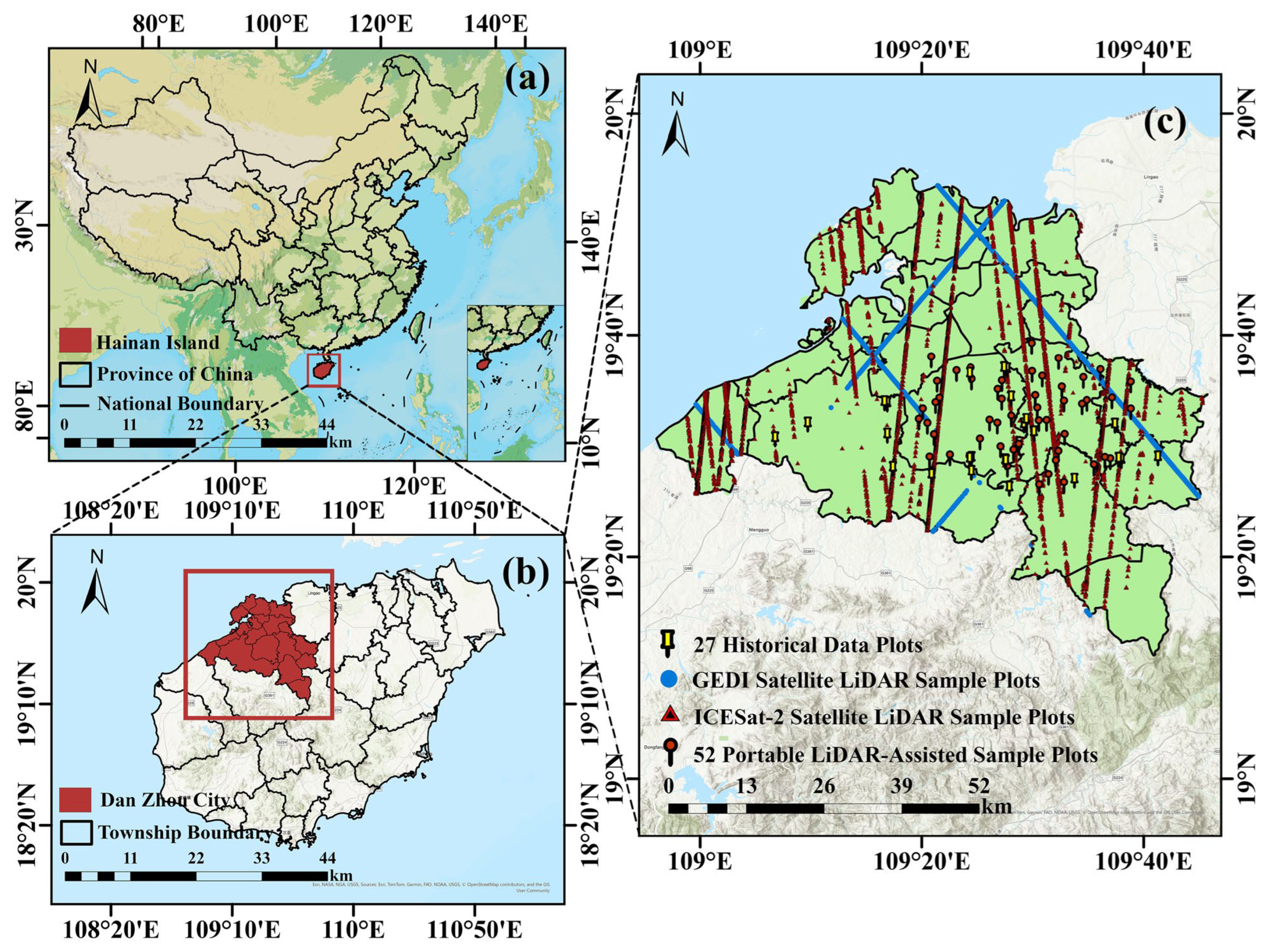
Danzhou City, Hainan Province, is in the hilly northwest region of Hainan Island (latitude 19°20′–19°52′, longitude 108°45′–109°40′). The terrain is gently undulating and primarily consists of low mountains, hills, tablelands, and plains. The average altitude is 100–400 m (Figure 2). The region has a tropical monsoon climate, with high temperatures, abundant rainfall throughout the year, and distinct dry and wet seasons. The soil is primarily composed of brick-red loam formed by the weathering of granite, with deep soil layers, good water permeability, and rich organic matter, which is suitable for the growth of tropical perennial crops. The superior climate and soil conditions provide a favorable ecological foundation for rubber trees. Danzhou City, the area with the most concentrated rubber plantations and the largest planting area on Hainan Island, holds an essential position in the natural rubber industry of the Province and China as a whole.

2.2. Data

2.2.1. Sentinel 2 Satellite Images

The data used in this study is derived from the Sentinel-2 surface reflectance product generated by the Google Earth Engine (GEE) platform. By setting a cloud cover threshold (≤20%) and combining it with the QA60 band for a secondary cloud masking process, image quality is ensured. The study period is from 2019 to 2024, and the image data for each year is selected from 1 March to 31 October. A synthetic method is used to obtain data for the 10 optical bands used for the analysis of vegetation indices and texture features.

2.2.2. Field Data

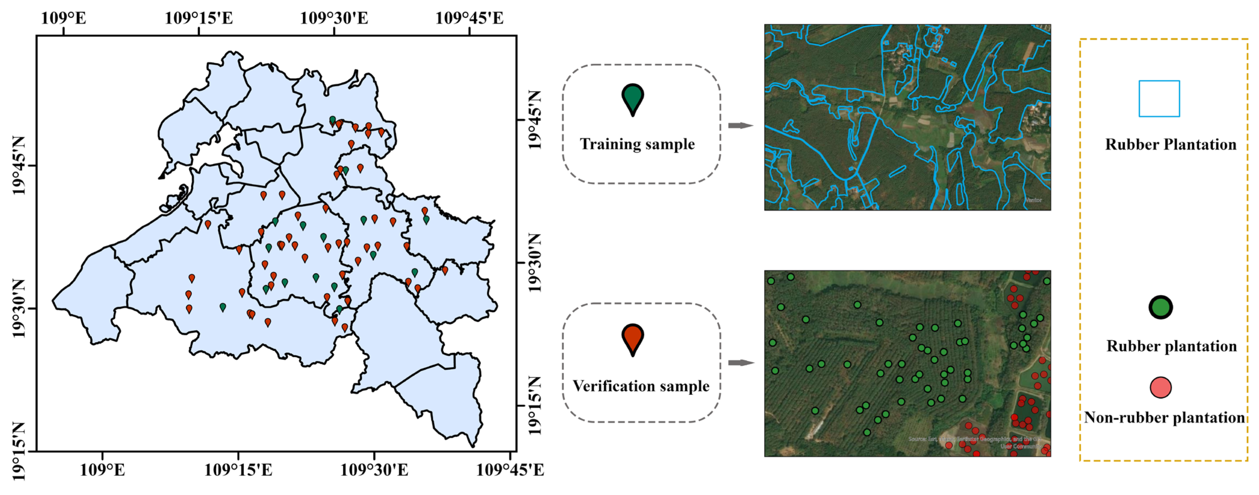
The rubber plantation distribution data used in this study primarily originated from a field survey conducted by the research team in 2020. This data is mainly used for the identification of rubber plantation distribution. The survey area is shown in Figure 3. A total of 67 areas were investigated. Training samples for model training were collected from 16 of the survey areas. This resulted in a total of 1826 training samples, each with a resolution of 128 × 128 pixels and a pixel size of 10 m. The remaining areas collected 2335 rubber plantation distribution points. To further supplement the data, 27 sample plots were set up in Danzhou City in 2023 (these are presented as historical data in the text); subsequently, from April to May 2024, 52 sample plots were randomly set up in Danzhou City for on-site investigation, and to verify and expand on the preliminary data (Figure 2). Each sample plot was 10 × 10 m. Handheld GPS (GPSMAP 63csx, Garmin, Olathe, KS, USA) and high-resolution images provided by Google Earth (Google, Santa Clara County, CA, USA) were used to complete on-site positioning and data collection. Additionally, the selection of 79 sample plots covered 7 towns: Dacheng Town, Heqing Town, Lanyang Town, Nada Town, Nanfeng Town, Wangwu Town, and Yaxing Town. The rubber plantation area in these towns accounted for more than 90% of the total area, and the distribution area of rubber plantations remained relatively stable from 2019 to 2023. This indicates that the rubber planting environment in these areas has strong continuity and stability. Therefore, choosing these areas as the source of sample collection not only ensures the representativeness of the samples but also guarantees the consistency of the data, reflecting the uniformity of the spatial distribution of rubber plantations.
A Velodyne VLP-16 laser scanner (Velodyne Corporation in San Jose, CA, USA) was used to obtain three-dimensional structural information for the forest stand. The point cloud data was processed using the Lego_LOAM algorithm, and the height and diameter information for the rubber forests in the sample plots were extracted in the Ubuntu RViz environment. Canopy height data were obtained from 52 sample plots using the unmanned aerial vehicle (UAV), the DJI Mavic 3M (DJI Innovation Company, Shenzhen, China), with a flight height of 60 m and real-time dynamic positioning (RTK) enabled, covering an area of 1.54 km2. The data was reconstructed into a DOM, DSM, and a three-dimensional point cloud using the DJI Terra 3.9.2 software, and canopy height was extracted based on the DSM and point cloud.

2.2.3. Spaceborne LiDAR Data

The ICESat-2 satellite was launched in October 2018, carrying the ATLAS system that employs single photon detection technology, significantly enhancing the accuracy of elevation data collection [25]. The satellite data can be freely accessed using NASA Earthdata Search (https://search.earthdata.nasa.gov; last accessed date: 10 April 2025). This study extracted canopy height data from the ATL08 version product. It ensured data quality through multiple levels of screening: excluding weak beam data (atlas_beam_type = weak), nighttime observation data (night_flag = 0), and data with high uncertainty (b_canopy_uncertainty = 3.4028235 × 1038); eliminating data with a canopy photon ratio of <5% (canopy_m_conf = 0), data affected by clouds and aerosols (cloud_flag_atm ≥ 2), and areas with a surface elevation deviation from the SRTM digital elevation model exceeding 50 m. Finally, only valid data within the Dianzhou area was retained for subsequent analysis. After screening, three percentiles of canopy height values (RH95, RH98, and RH100) were selected to model the canopy height in Dianzhou, Hainan Island.
The GEDI satellite, launched by NASA in December 2018, generates eight parallel observation orbits using three laser devices, providing high-resolution forest structure data [26]. This study used the second version of the GEDI L2A dataset, which can be freely accessed through NASA Earthdata Search (https://search.earthdata.nasa.gov; last accessed date: 10 April 2025). To ensure data reliability, the study used multiple screening criteria: first, data points were filtered within the study area based on longitude and latitude values (lon_lowestmode_a<n> and lat_lowestmode_a<n>); second, only data with a quality flag of 1 (quality_flag_a<n> = 1) were retained, and samples with a height difference of >50 m from TanDEM-X were excluded. To eliminate errors caused by cloud interference, we removed invalid data where the absolute difference between elevation and TanDEM-X was >50 m. The subsequent filtering process included: removing degraded data (degrade_flag = 1), excluding observation points with a sensitivity of <0.9, and ensuring algorithm integrity by retaining data with an “rx_algrunflag” value of 1. After screening, the canopy height percentiles of RH95, RH98, and RH100 were used to model the canopy height in Danzhou City, Hainan Island.
After screening the initial data points obtained from ICESat-2 and GEDI, a total of 3173 valid samples were retained in this study.

2.2.4. Terrain Feature Data

The ALOS satellite DEM data (with a resolution of 12.5 m) provided by the NASA Earth Science Data website (https://search.asf.alaska.edu; last accessed on 15 April 2025) was analyzed using ArcGIS Pro 3.4.0 to extract the slope and aspect information for Danzhou City. To ensure data consistency, the slope, aspect, and DEM data were uniformly resampled to a resolution of 10 m using the three-pass convolution resampling method.

2.2.5. Climate Data

The historical annual average temperature and precipitation data for the study area, from 2019 to 2024, were obtained from the National Earth System Science Data Center of the United States (https://www.geodata.cn; last accessed on 1 May 2025), with a spatial resolution of 1 km. To enhance the data details and consistency, the resolution of the data was uniformly adjusted to 10 m with three convolution resampling.

2.3. Methods

The main hardware configuration used in this study is an Intel Core i7-13700K processor (16 cores, 24 threads, with a maximum boost frequency of 5.40 GHz) and a NVIDIA GeForce RTX 4080 (16 GB of video memory).

2.3.1. Multi-Rule Synthesis and Deep Learning Integration Method for Remote Sensing Images

The “qualityMosaic()” function in the GEE platform was used to select the best pixels for synthesis from multiple time-series images. Pixels with the highest values based on the quality parameters were chosen to generate a single image. Three spectral indices, KNDVI, NDVI, and LSWI, were selected for this study. NDVI is used to reflect the growth status of vegetation [27], LSWI is used to monitor vegetation and soil moisture [28], and KNDVI, as a nonlinear improvement index of NDVI, effectively alleviates the saturation problem in high coverage areas and enhances the sensitivity and accuracy in reflecting vegetation greenness and biomass [29]. From the vegetation spectral radiative transfer model perspective, traditional NDVI saturates in high-coverage areas, as reflectance changes stabilize with increased vegetation, limiting NDVI’s sensitivity. However, KNDVI nonlinearly adjusts the red and near-infrared reflectance, effectively capturing changes in high-coverage areas, thus avoiding saturation and improving sensitivity and accuracy. This makes KNDVI better at distinguishing areas with high biomass and greenness, making it more suitable for ecological monitoring and agricultural remote sensing analysis. The annual median composite was also used to generate remote sensing images of rubber plantations to represent their typical state. All processing was completed in the GEE platform (the index synthesis method is shown in Table 1).
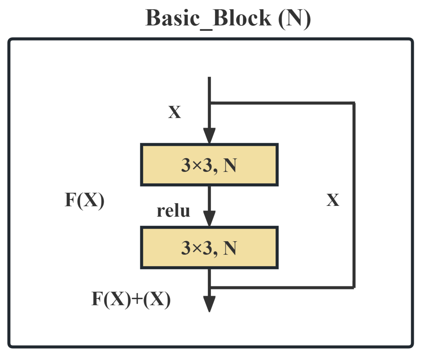
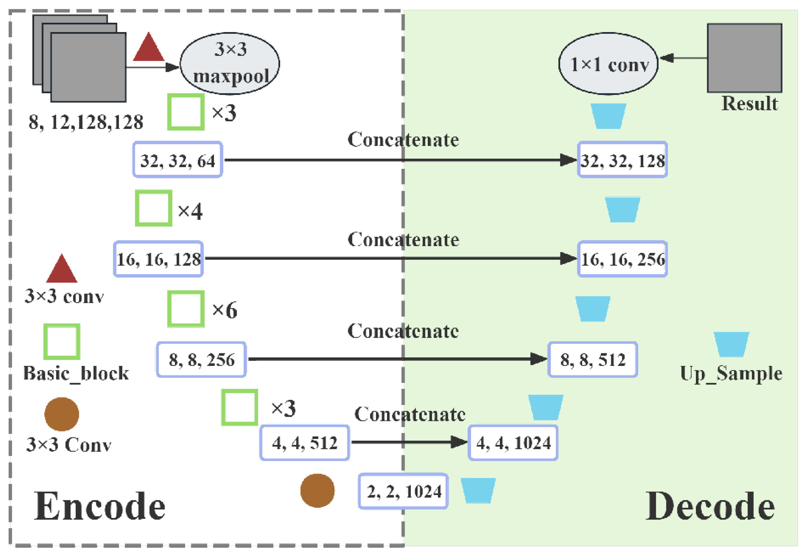
This study employs a variant of Res34_Unet based on the U-Net structure for pixel-level classification of rubber plantations [30]. U-Net enhances classification capabilities through multi-scale feature extraction and skip connections that fuse feature information from different levels. To improve feature extraction capabilities and training stability, ResNet34 is used instead of the U-Net encoder, leveraging its advantages in deep residual networks to address the issues of gradient vanishing and degradation. Res34_Unet extracts multi-dimensional features through progressive dimensionality reduction and upsamples to restore spatial resolution during decoding, while fusing the features from the encoder, further improving classification accuracy and stability. The feature extraction module is constructed using ResNet34, and its specific architecture is shown in Figure 4. The Res34_Unet module follows the U-Net structure, as shown in Figure 5. The model is trained using the Adam optimizer, with 1000 epochs, an initial learning rate of 0.01, a batch size of 8, and the optimizer is renowned for its excellent performance and convergence speed. The parameter update formula is shown in Equation (1):
θ t θ t 1 γ m t ^ ( v t ^ + ϵ )
where t is the current training step; θ t is the model parameter (such as weight or bias) at step t, and θ t 1 is its value at the previous step; m t ^ and v t ^ are the bias-corrected first-order and second-order moment estimates of the gradients, respectively, which are used to adaptively scale the learning rate for each parameter; and ϵ is a small constant introduced to prevent division by zero.
Rubber plantation classification is a binary process. However, due to the significant difference in the number of rubber plantation and non-rubber plantation samples, the data distribution becomes extremely unbalanced, causing the model to tend to favor the majority class samples during training, thereby affecting the recognition performance of the minority class (rubber plantations). To address this issue, this study proposes two optimization strategies: mixed sample augmentation (Mixup) and weighted cross-entropy loss function (Weighted Cross-Entropy Loss). Mixup generates new training samples through linear interpolation of the samples, effectively reducing the risk of overfitting of the model to a single sample and enhancing the model’s robustness to noise and unseen data [31]. Its core idea can be expressed in Equations (2)–(4); the weighted cross-entropy loss function assigns different weights to different classes, increasing the weight of minority class samples in the loss function and enhancing the model’s learning ability in small sample classes. The combination of the two effectively alleviates the overfitting problem and improves the classification accuracy and robustness of the model. The mathematical definitions are shown in Equations (5) and (6).
X ~ = λ x i + ( 1 λ ) x j
Y ~ = λ y i + ( 1 λ ) y j ,
f ( λ α , β ) = 1 B ( α , β ) λ a 1 ( 1 λ ) β 1
In the formula, the mixed sample is denoted as X, and the corresponding label is Y. xi,yi and xj,yj are randomly selected samples from the training set, λ is a random number, B(α,β) is the Beta function, and α and β are the parameters of the Beta distribution.
ω c = 1 log ( ϵ + f c )   ,
L = c = 1 C ω c y c log y c ^ ,  
In the formula, ω c represents the weight of category c , f c represents the pixel frequency of category c , and ϵ is a constant used to avoid division by zero errors.
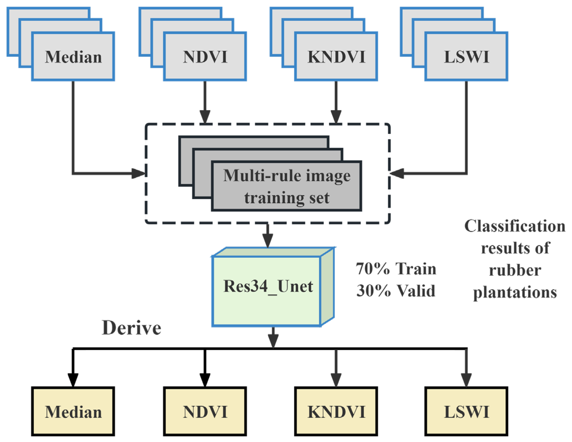
To integrate deep learning models with multi-rule remote sensing composite images, we constructed an overall framework, as shown in Figure 6. Specifically, the 2020 remote sensing images synthesized by KNDVI, NDVI, LSWI, and the median rule, along with their corresponding labels, are used as a unified input to train a single model, rather than modeling different rules separately. During the training process, all types of synthetic images are divided into training and validation sets in a 7:3 ratio to ensure consistent data usage. After model training is completed, the remote sensing datasets were synthesized using each rule, and the resulting inferences were successively inferred.

2.3.2. Multi-Rule Remote Sensing Image Deep Learning Fusion

For internal validation, we constructed four deep learning models, RB_2020_KNDVI, RB_2020_NDVI, RB_2020_LSWI, and RB_2020_Median. A 30% validation set was used to evaluate the model’s generalization performance on the existing data. The validation process is primarily based on three indicators: precision, recall rate, and F1-score, as shown in Equations (7)–(9):
P recision = TP TP + FP ,
Recall = TP TP + FN ,
F 1 - score = 2 × TP TP + FP + TP + FN   ,
Precision is used to measure the proportion of pixels predicted as rubber plantations that are actually rubber plantations, which is of great significance in applications with high precision requirements. The recall rate indicates the proportion of rubber plantation pixels that are correctly identified; a high recall rate suggests that the model can cover more rubber plantation areas. The F1-score is equivalent to a dice factor and can effectively evaluate the performance of the model as an image classification tool. To facilitate the understanding of each parameter, explanations for the symbols are provided in the table (Table 2).
External validation is used to test the generalization ability of the model under different environments and data conditions, and evaluate the prediction accuracy and performance stability of the model in situations beyond the training samples. To quantify the model’s classification performance, a confusion matrix (Table 3) is constructed, and the user accuracy, producer accuracy, overall accuracy, and Kappa coefficient are calculated to comprehensively reflect its performance as a classifier of rubber plantations and non-rubber plantations. Of the samples, 30% were selected as validation samples. The validation samples are divided into rubber plantations and non-rubber plantations, and each sample has a resolution of 128 × 128 pixels with a pixel size of 10 m.
User accuracy is used to measure the correctness of the model’s identification of rubber plantations, while producer accuracy reflects its ability to exclude non-rubber plantations; overall classification accuracy (OA) represents the overall classification level, and the Kappa coefficient tests the consistency between the classification results and the actual situation [32]. The specific calculation formulas are shown in Equations (10)–(12).
OA = a + d a + b + c + d ,
kappa = OA     P e   1     P e ,
P e = ( a + b ) × ( a + c ) + ( c + d ) × ( b + d ) ( a + b + c + d ) 2 ,
In a confusion matrix, ‘a’ represents true positive, ‘b’ represents false positive, ‘c’ represents false negative, and ‘d’ represents true negative. In the formula, ‘pe’ represents the random consistency probability, which is the probability that the classifier is coincidentally consistent with the true results in a completely random classification scenario, and is used for the correction calculation of the Kappa coefficient [33].

2.3.3. Selection of Characteristic Factors

Before modeling, feature data related to the target variable were obtained, but each feature contributed differently to the prediction performance. Consequently, feature selection was required. The Spearman rank correlation coefficient, as a non-parametric statistical method, can effectively measure the monotonic correlation between variables and is suitable for non-normal or ordinal data analysis [34]. In this study, the Spearman coefficient was first used to evaluate the correlation between each feature and the dependent variable (canopy height, biomass), and key features were selected after sorting based on the absolute value of the coefficient. The variance inflation factor (VIF) was then used to diagnose collinearity. The VIF measures the degree of variance expansion when a feature is present along with other features. A higher VIF value indicates a strong correlation between features, which may lead to unstable models. To ensure the stability of the model, we set the VIF threshold at 10. Features with a VIF > 10 were considered to have severe collinearity and were excluded.
The results of the selected feature factors are listed in Table 4.

2.3.4. Model Construction

To model rubber plantation canopy height amongst 3173 samples, four typical machine learning algorithms were selected: BP, RF, GBDT, and XGBoost. The data were divided into an 8:2 ratio of training and test data to evaluate the model’s performance. Tree height data for 937 points was extracted by drones and used for external validation to assess the model’s generalization ability and applicability.
Five algorithms (BP, RF, CNN, GBDT, and XGBoost) were used to model plantation biomass using data obtained from 52 sample plots in 2024 and 27 historical sample plots in 2023. The introduction of historical sample plots expanded the sample size and representativeness, improving the robustness and generalization ability of the model. The data were divided in an 8:2 ratio of training and test data, respectively, to assess model fitting and testing, and the performance of each algorithm in biomass estimation was compared using the external validation system.
The CNN algorithm extracts remote sensing features through convolution, pooling, and fully connected layers [35]. The biomass modeling uses 16/32 filters, a 32-neuron fully connected layer. To reduce overfitting, a 20% dropout is applied in the model. During training, the SGDM optimizer is used with a batch size of 8, and the maximum number of training epochs is set to 100.
The RF algorithm is a powerful machine learning algorithm that has been widely used for classification, regression, and clustering [36]. The canopy height model uses 100 decision trees with a minimum leaf node number of 10; the biomass model uses 200 decision trees with a minimum leaf node number of 3 to accommodate different modeling requirements. All models are trained using the Bootstrap resampling method for each decision tree, and the predictions from multiple trees are integrated to enhance the model’s robustness and generalization ability.
The BP algorithm is a classic feedforward neural network trained via backpropagation [37]. The canopy height model uses 300 iterations, an error threshold of 1 × 10⁻¹⁹, and a learning rate of 0.0001 to ensure stability and accuracy; the biomass model uses 600 iterations, an error threshold of 1 × 10⁻⁵, and a learning rate of 0.01 are used to suit biomass prediction convergence and modeling needs.
The GBDT algorithm optimizes the prediction results through multiple decision trees and can effectively depict complex nonlinear relationships [38]. The canopy height model uses 300 trees, a maximum split number of 10, and a learning rate of 0.1; the biomass model uses 200 trees, a maximum split number of 5, and a learning rate of 0.01 to improve prediction stability.
XGBoost is an efficient ensemble learning algorithm optimized using GBDT, with high computational efficiency and excellent prediction performance [39]. The canopy height model and the biomass model uses 200 weak learners, with a learning rate of 0.05, a maximum tree depth of 2, and set L1 regularization coefficient 2.0 and L2 regularization coefficient 2.0 to control the model complexity. The objective function is the squared error regression.
In this study, the RF, BP, CNN, and GBDT algorithms were all implemented using Matlab 2024, whereas the XGBoost algorithm used the xgboost library with the PyCharm 2025.2.0.1 platform. By achieving cross-platform implementation of different algorithms, we not only ensured the stability and reproducibility of the model operation but also guaranteed the reliability of the multi-algorithm comparison analysis.

2.3.5. Model Evaluation and Validation

Model performance was evaluated using five indicators: coefficient of determination (R2), bias, relative bias, root mean square error (RMSE), and relative root mean square error (RRMSE). These indicators can comprehensively reflect the fitting accuracy and predictive ability of the model from different perspectives.
R2 is used to measure the degree to which the model explains the variance of the observed data [40]. Bias is used to assess the systematic error between the predicted values and the observed values. Relative bias represents the proportion of the bias relative to the observed values [41]. RMSE represents the average error magnitude between the predicted values and the observed values and RRMSE reflects the relative size of the error by calculating the ratio of RMSE to the mean of the observed values [42]. The specific calculation formulas are as follows (13)–(17):
R 2 = 1 i = 1 n ( y i y i ^ ) 2 i = 1 n ( y i y - ) 2 ,
Bias = 1 n i = 1 n ( y i ^ y i ) ,
Bias % = Bias y - × 100 % ,
RMSE = 1 n i = 1 n ( y i ^ y i ) 2 ,
RRMSE = RMSE y - × 100 % ,
where y - is the average value of the true values, y i is the true value of the i-th sample, y i ^ is the predicted value of the i-th sample, and n represents the total number of samples.

3. Results

3.1. Rubber Plantation Recognition and Spatiotemporal Evolution Analysis Based on Multi-Rule Remote Sensing Images and Deep Learning Models

3.1.1. Multi-Rule Remote Sensing Images

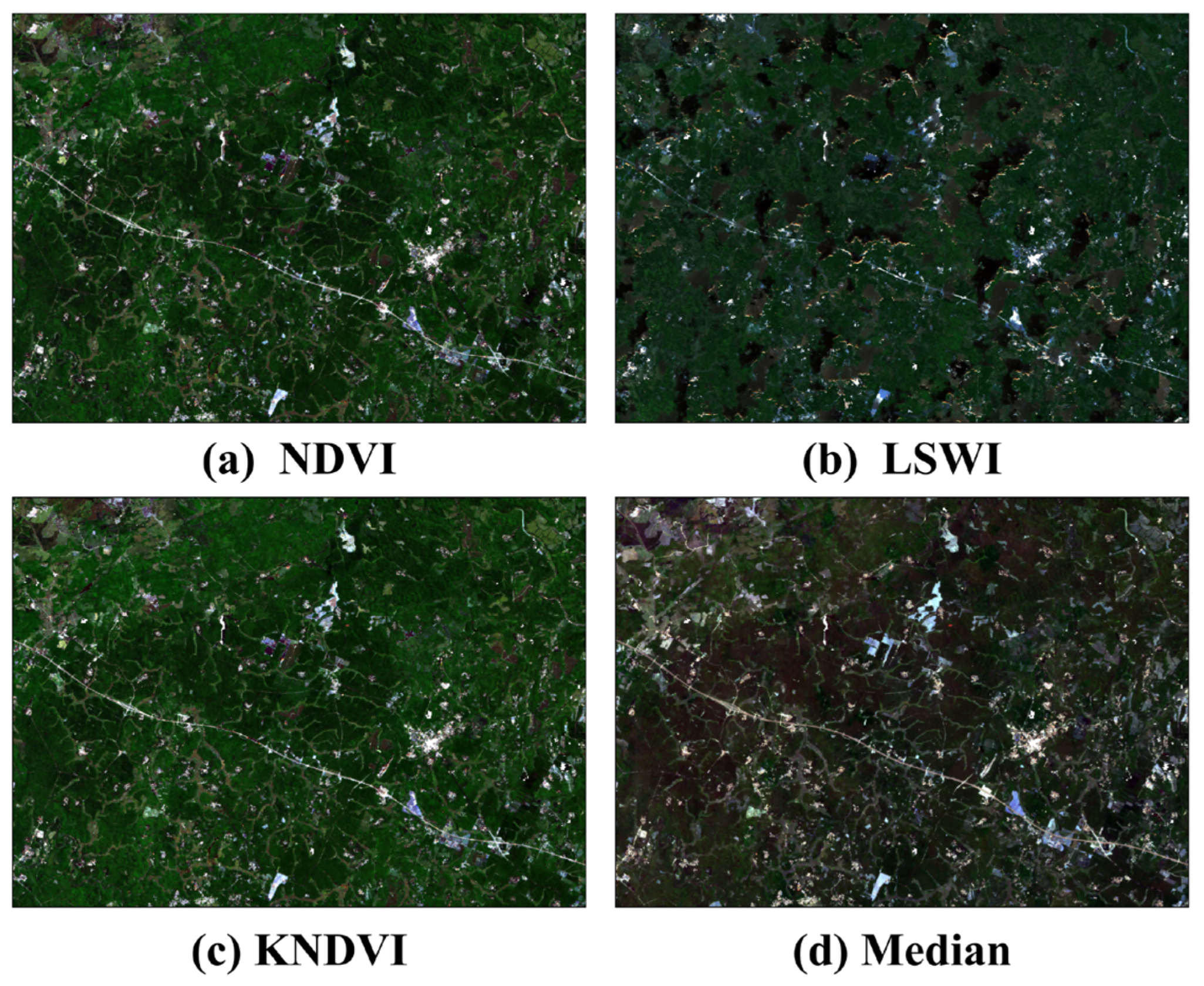
Remote sensing images of typical areas in Danzhou City were synthesized and classified using different rules (Figure 7). The images synthesized using KNDVI and NDVI highlight the growth status of vegetation and reflect the spatial differences in regional vegetation; the median synthesized images present the common growth state of vegetation more intuitively. In contrast, the images synthesized using LSWI are affected by cloud interference. However, this interference does not directly cover the spectral vegetation information, and consequently, vegetation features can still be identified.

3.1.2. Model Training Results and Internal Validation

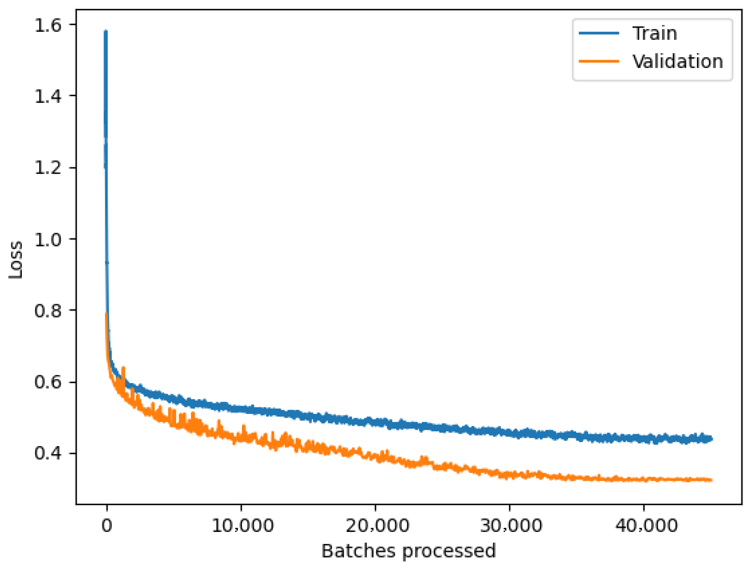
Among the various models constructed, RB_2020_KNDVI performed the best. The trend for loss of function during the training process is shown in Figure 8. At the beginning of the training process, the loss values of the training and validation sets were relatively high. They rapidly decreased as the number of iterations increased, indicating that the model can effectively extract features. Overall, the loss value of the validation set was always lower than that of the training set, and both tended to stabilize in the later stages, converging at approximately 0.35 and 0.42, respectively. This result indicates that the model did not show significant overfitting during the training process and has strong generalization ability, providing a reliable prediction basis for subsequent analysis.
The internal validation results for the four models are presented in Table 5. For non-rubber plantation targets, the RB_2020_KNDVI model achieved an accuracy rate, recall rate, and F1 score of 0.95, respectively. However, for rubber plantation targets, the corresponding rates were 0.92, 0.93, and 0.92, respectively. Overall, the RB_2020_KNDVI model demonstrated outstanding performance as a rubber plantation classifier.

3.1.3. Comprehensive External Validation and Evaluation of Model Performance

The classification results from the RB_2020_KNDVI model demonstrated high external validation accuracy (Table 6 and Table 7). The confusion matrix results indicated that the model could effectively distinguish between rubber plantations and non-rubber plantations, with a total accuracy rate of 91.63% and a Kappa coefficient of 0.83, indicating that the model’s classification results were highly consistent with the actual data. Further analysis revealed that the producer’s precision for rubber plantations was 89.63%, and the user’s precision was 90.18%, indicating that the model achieved a balance between high recognition rates and reliability when extracting data on rubber plantations. The producers’ and users’ precision for non-rubber plantations were 93.04% and 92.63%, respectively, both higher than those for the rubber plantations. This suggests that the model’s identification of non-rubber plantations is more stable than that of rubber plantations; however, both detection rates are relatively high. Overall, this model demonstrated an excellent external generalization ability for the identification of rubber plantation distributions and will provide reliable support for subsequent regional-scale rubber plantation monitoring.
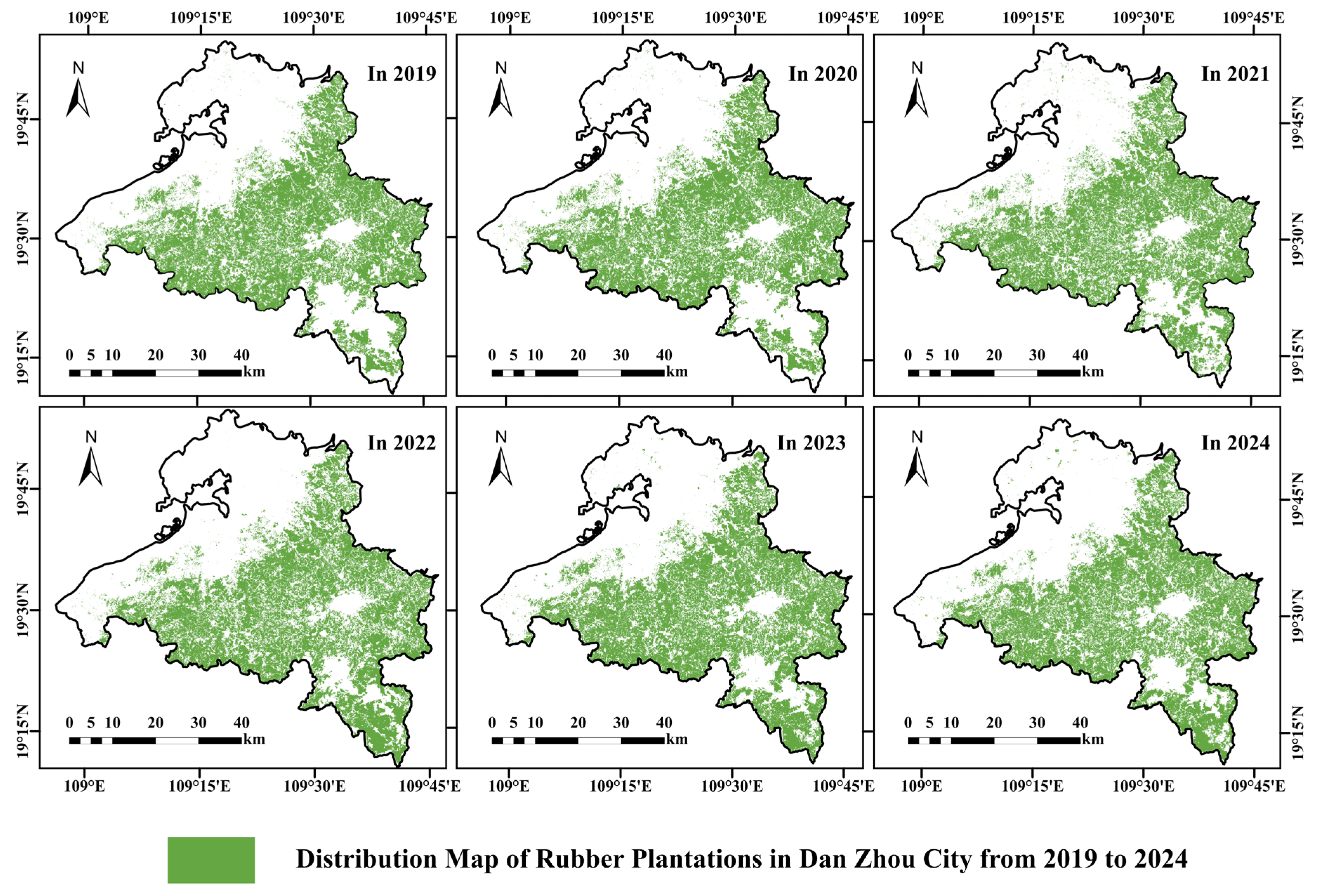
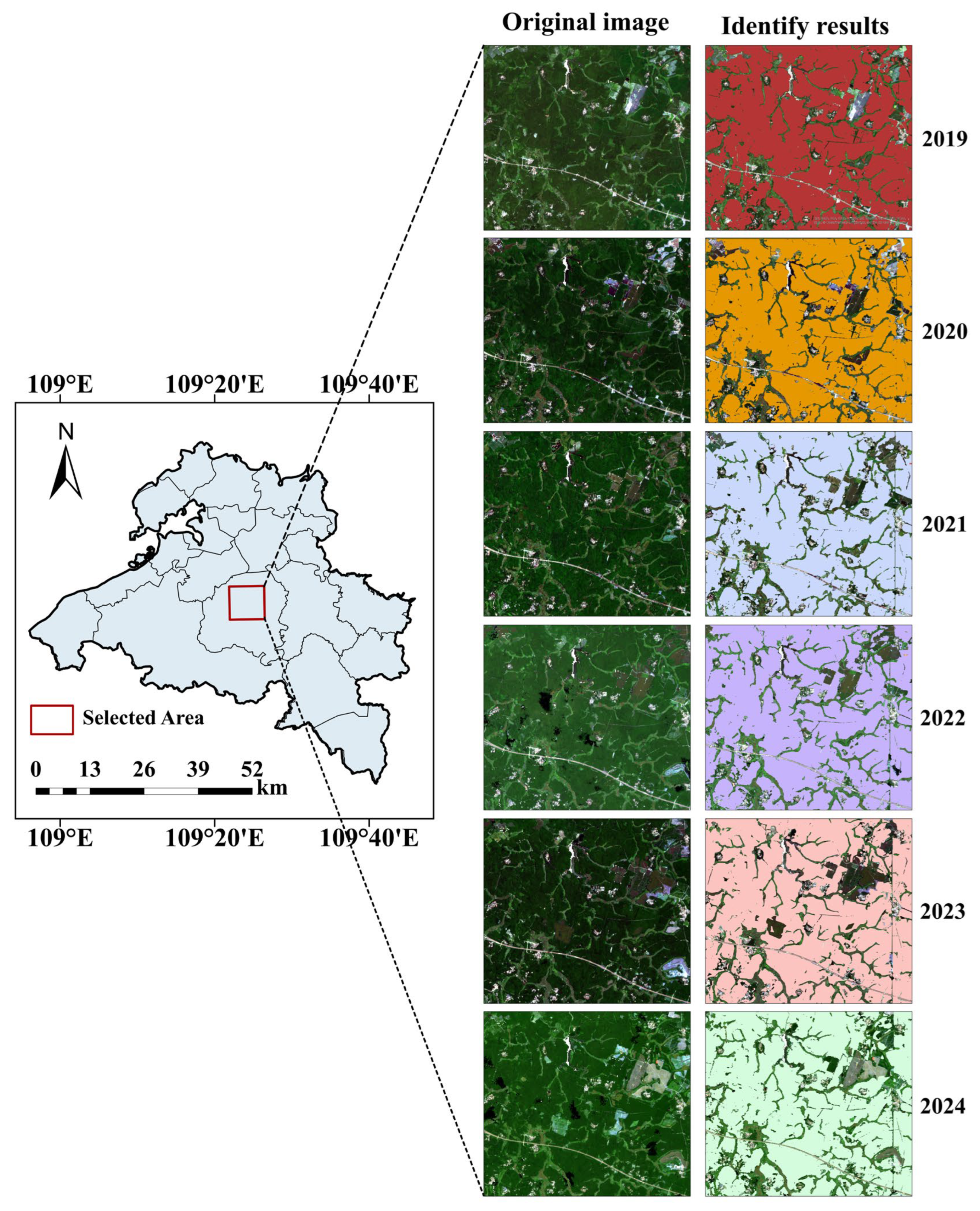
The spatial patterns and dynamic changes of typical rubber plantation areas in Danzhou City from 2019 to 2024 are shown in Figure 9. The identification results for each year are highly consistent with the original images, indicating that the model can stably capture the spatial distribution characteristics of the rubber plantations. The temporal comparison reveals an expansion trend for the rubber plantations during the study period, along with local fragmentation and edge degradation phenomena, highlighting the complexity of the regional forest stand’s dynamic evolution.

3.1.4. Spatiotemporal Changes in the Rubber Plantation Area in Danzhou City

A distribution map of rubber plantations in Danzhou City from 2019 to 2024 is presented in Figure 10, which clearly illustrates the overall spatial pattern of rubber plantations within the city area. The rubber plantations are primarily concentrated in the central, southeastern, and western regions of the city. While these areas are relatively stable overall, some peripheral areas have experienced contraction or substitution. The rubber plantation area in each town (district, Figure 10) was statistically analyzed (Table 8). The total rubber plantation area fluctuated from 2019 to 2024. In 2019, it was 134,836.45 hectares, reaching a peak of 144,253.01 hectares in 2023, and dropping to 138,109.81 hectares in 2024. Among them, Yaxing Town, Dacheng Town, and Nada Town are the core distribution areas. Furthermore, Lanyang Town has expanded significantly, and Dongcheng Town and Baimaijing Town have shown a downward trend.
Overall, the rubber plantation pattern remained relatively stable from 2019 to 2021. In 2022, some high-density areas began to decline, but by 2023–2024, the overall pattern had once again become stable. This temporal change feature indicates that although external disturbances have had some impact on local forest stands, the overall pattern of rubber plantations in Danzhou maintained a strong continuity and stability.

3.2. Accuracy Verification of the Remote Sensing Estimation Model for the Height of Rubber Plantations Canopies

Multiple rounds of training and parameter optimization were conducted for four types of machine learning algorithms. Their generalization ability and prediction accuracy were continuously improved through a comparative analysis of the training and test datasets. Internal validation was performed using randomly selected 20% test samples from the data not used for training to evaluate the model’s applicability. External validation was based on 937 independent tree height points obtained from an unmanned aerial vehicle (UAV) aerial survey to test the model’s generalization ability under new data conditions. The two types of validation results (Table 9 and Table 10) summarize the accuracy performance of different algorithms under percentile indicators, such as RH95, RH98, and RH100, thereby providing a clear comparison of the differences and advantages of each model in internal and external validations.
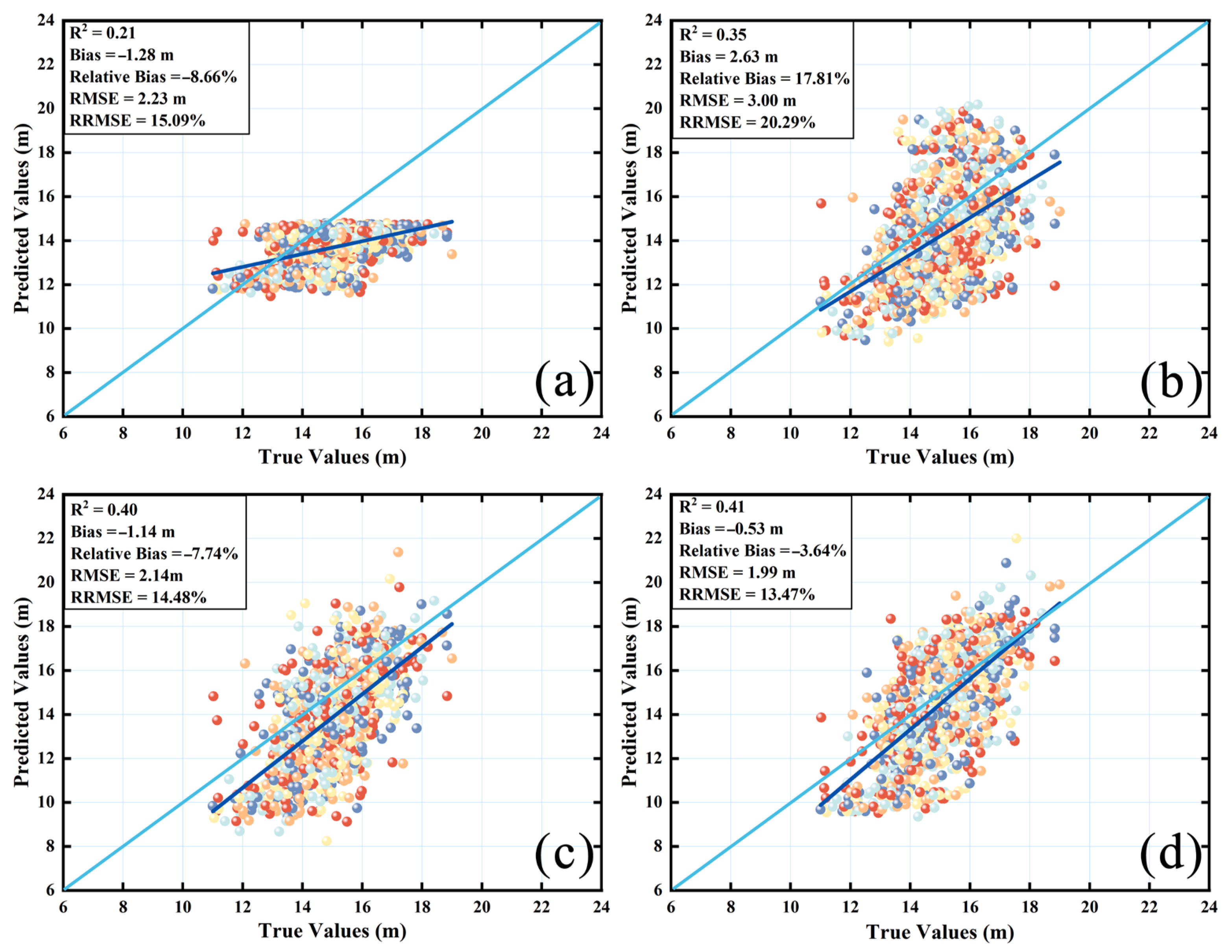
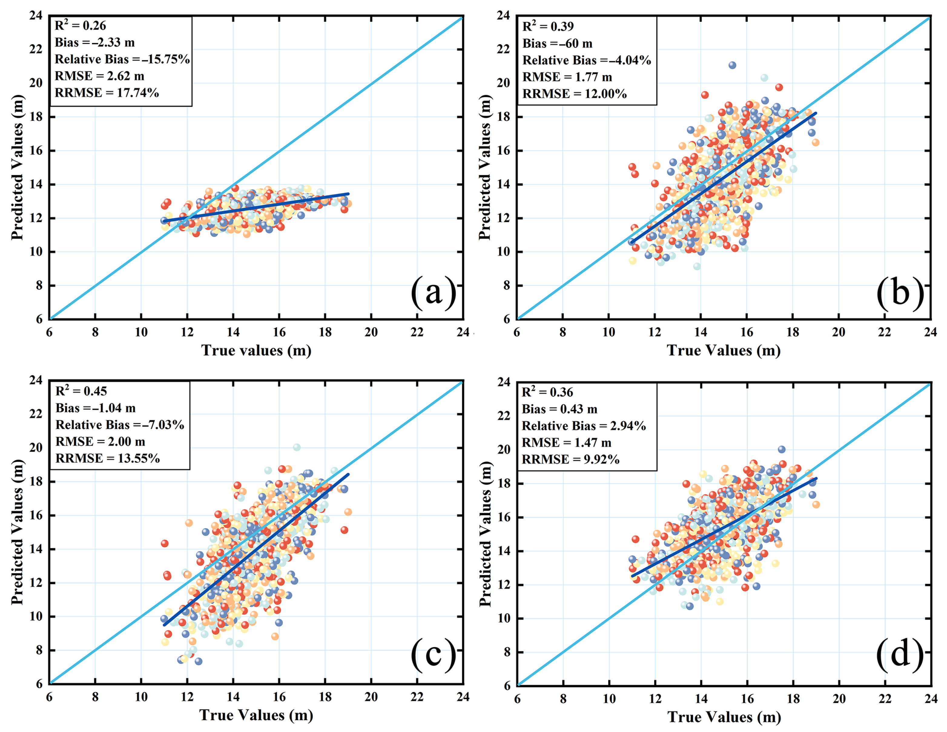
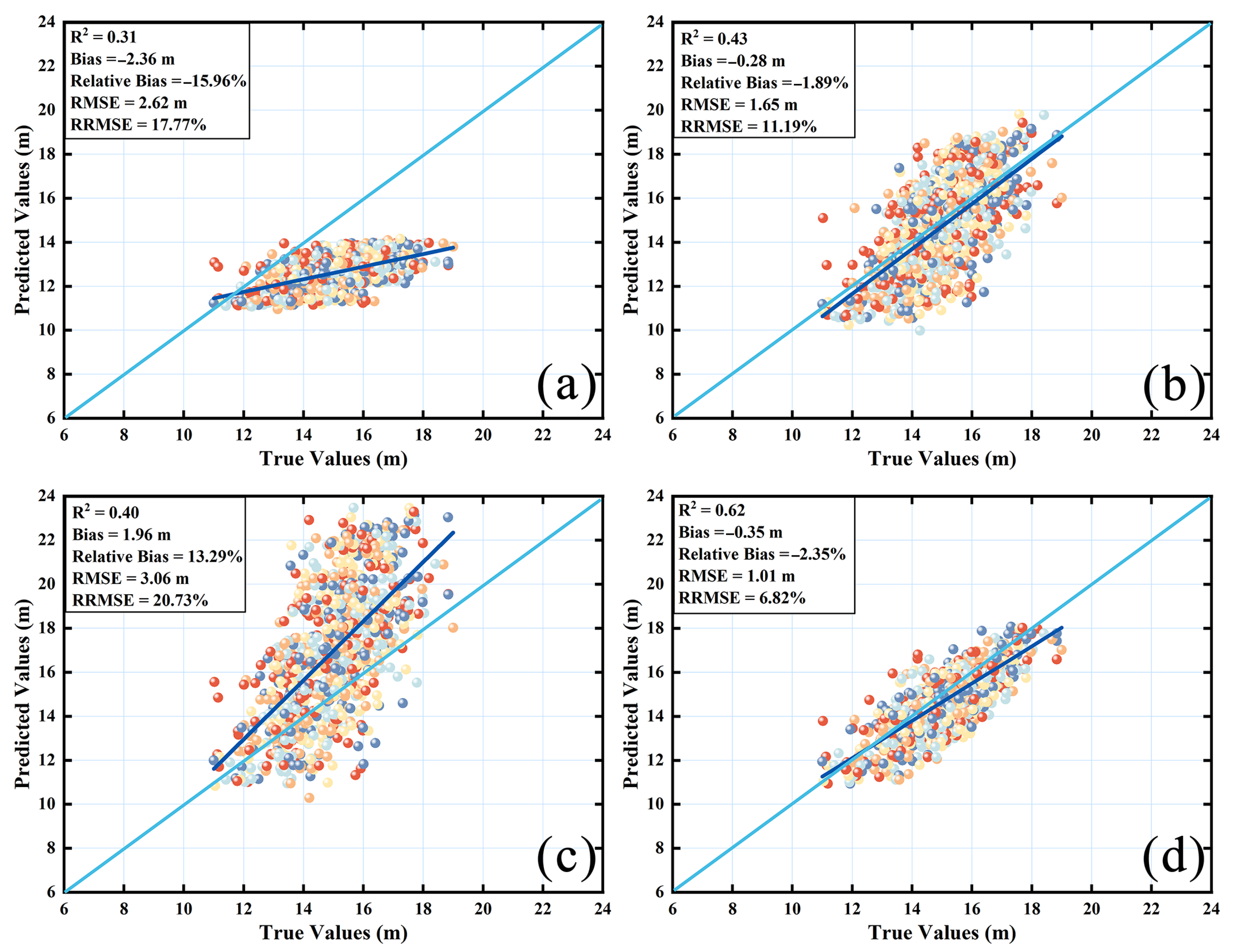
During the internal validation, the four machine learning algorithms showed specific differences at different percentiles. Overall, the BP model had lower fitting and prediction accuracy. RF and GBDT had higher R2 values with the training set, but performed relatively poorly with the test set, showing a certain overfitting phenomenon. In contrast, XGBoost maintained an R2 value > 0.60 with the test set, with a bias close to zero, and a relatively low RMSE and RRMSE, demonstrating strong stability and generalization ability. External validation results (Table 10) show that although each model had a certain degree of deviation and error under RH95 and RH98 conditions, XGBoost performed best under RH100 conditions, with an R2 of 0.62, a bias controlled at −0.35 m, and an RMSE and RRMSE of 1.01 m and 6.82%, respectively, significantly outperforming other models and percentile combinations. Overall, the XGBoost model under RH100 conditions demonstrated the best fitting accuracy and stability in both internal and external validations and was selected as the final canopy height estimation model.
To comprehensively evaluate the applicability of different percentile indicators (RH95, RH98, and RH100) as predictors of canopy height in rubber plantations, as well as the predictive capabilities of various machine learning models (RF, BP, GBDT, and XGBoost), external validation scatter plots were prepared to visually display the relationship between model predicted values and actual values (Figure 11, Figure 12 and Figure 13).

3.3. Changes in the Canopy Height of Rubber Plantations

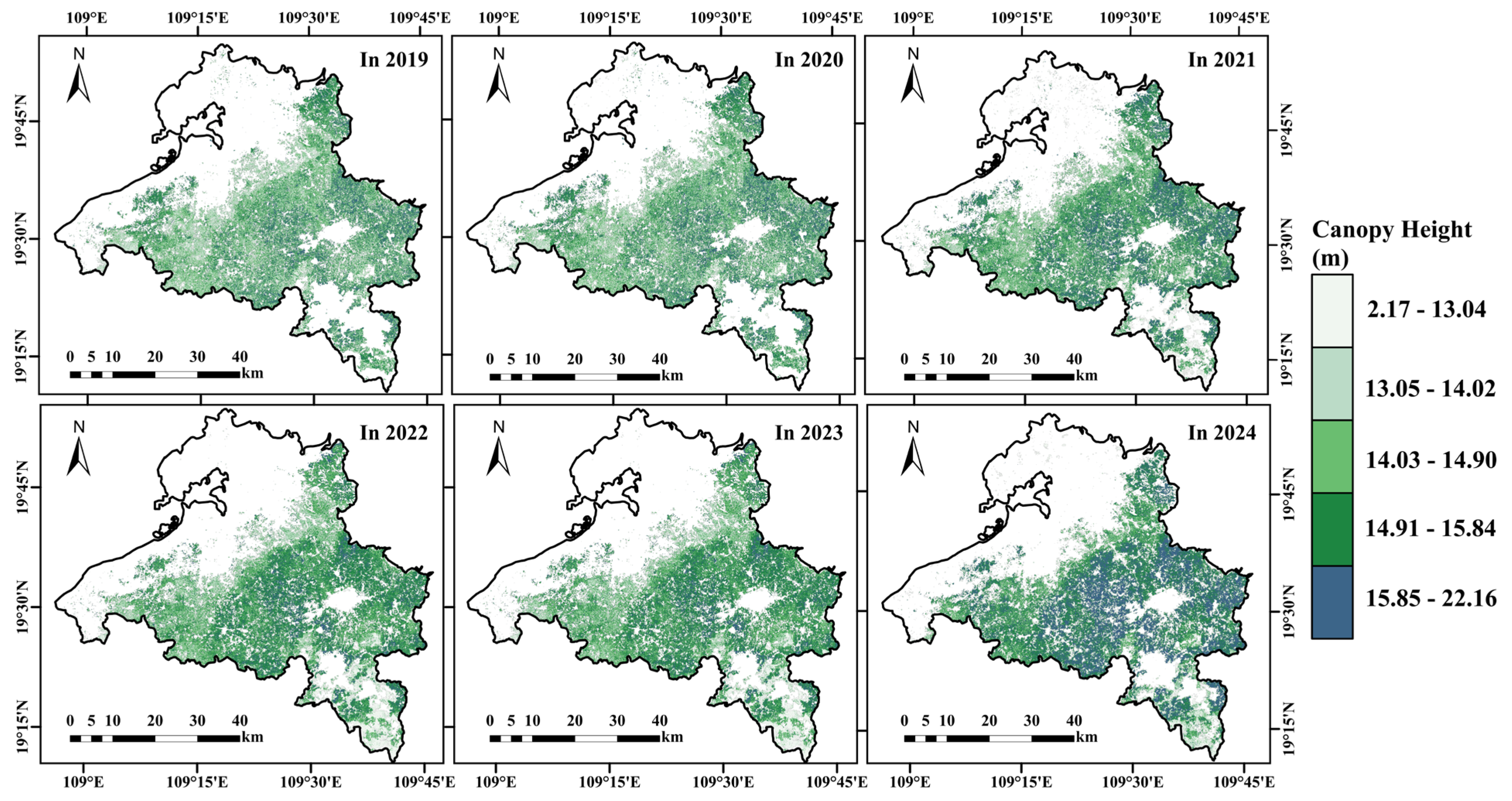
A canopy height estimation model based on the XGBoost algorithm was constructed, and the 100th percentile of RH100 was used as the prediction benchmark to invert the canopy height of rubber plantations in Danzhou City from 2019 to 2024. A canopy height distribution map with a spatial resolution of 10 m was generated (Figure 14).
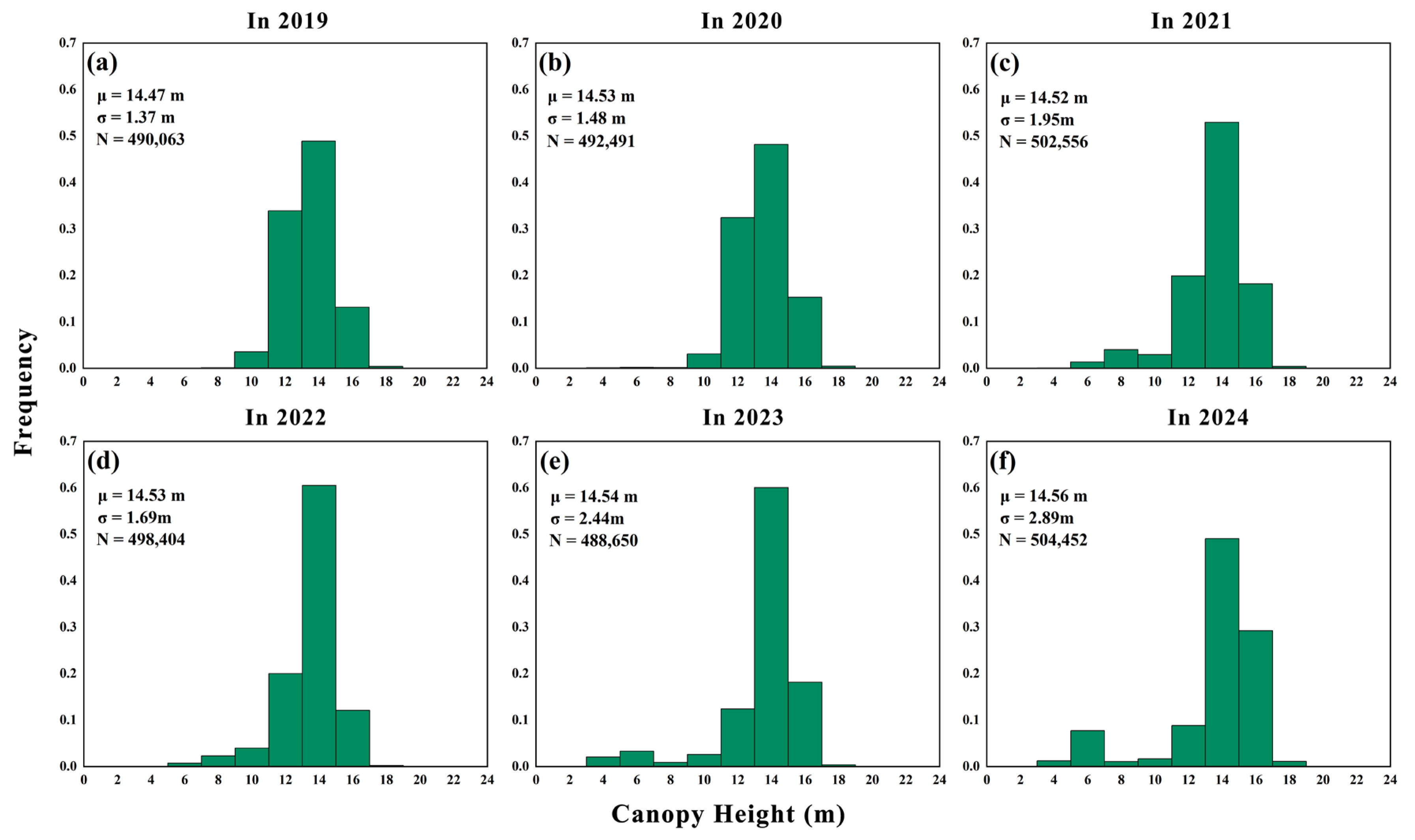
From 2019 to 2024, the canopy height in Danzhou City showed an increasing trend, and the spatial pattern underwent significant changes. From 2019 to 2020, the canopy height values throughout the city were low to medium, predominantly <13 m, with limited high-value areas. Since 2021, the canopy height has gradually increased, and the area with 14–16 m trees has expanded significantly. Some central and southeastern forest areas have presented continuous high-value segments. By 2023, the canopy height further increased, with local areas exceeding 16 m. In 2024, the canopy height generally reached 15–22 m, with the eastern and southern regions being particularly prominent.
Furthermore, this study also created a histogram of the tree canopy heights in rubber plantations (Figure 15), visually presenting the distribution of different canopy heights throughout the year. Through these histograms, one can gain a deeper understanding of the distribution frequency and changing trends of the tree canopy heights in rubber plantations over different years.

3.4. Accuracy Verification of the Remote Sensing Estimation Model for Rubber Plantation Biomass

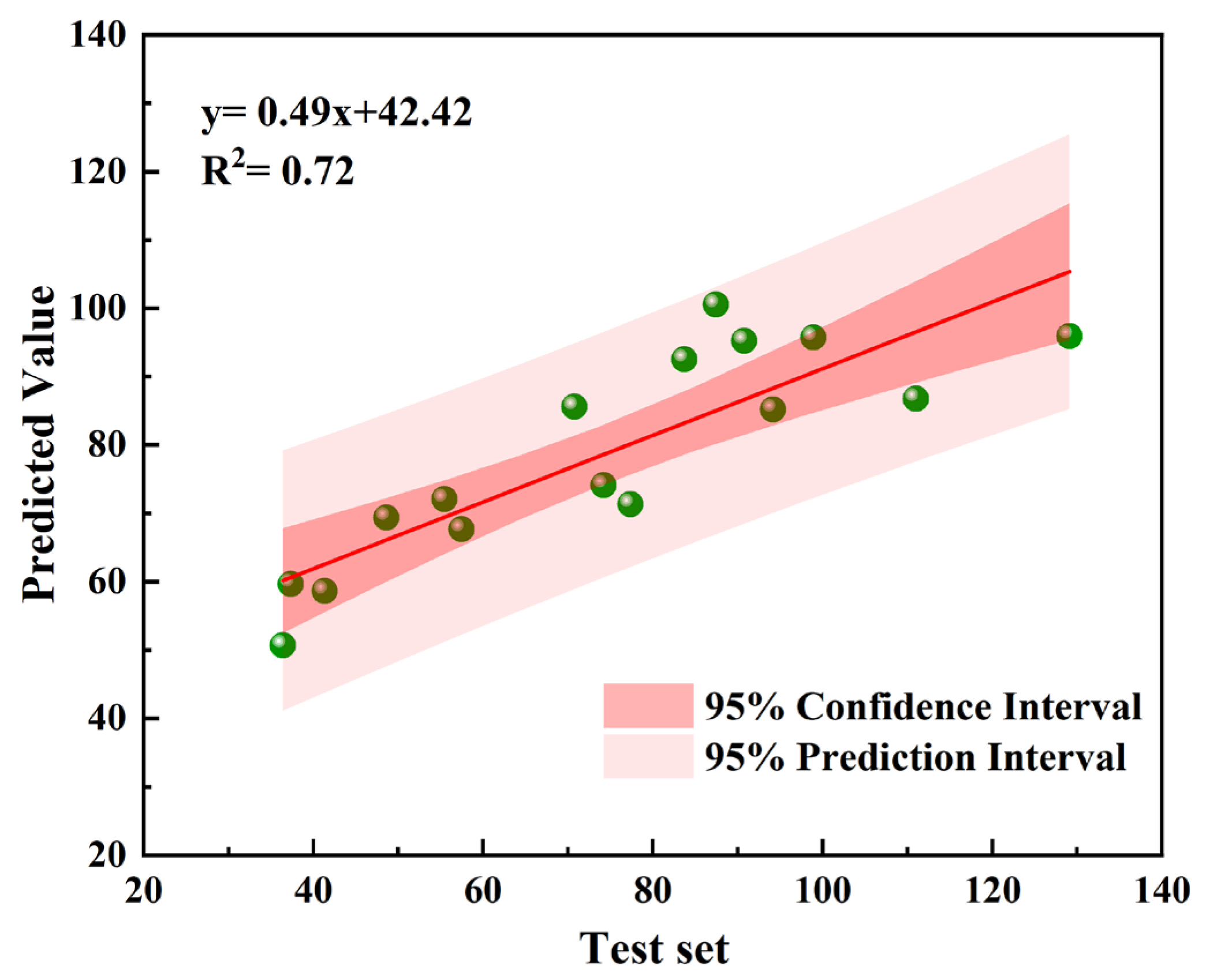
There are significant differences in the performance of each model in the remote sensing estimation of rubber plantation biomass (Table 11). The determination coefficients of BP and CNN are both relatively low (0.42 and 0.45, respectively), and both are accompanied by high RMSE and RRMSE, indicating that the fitting abilities and accuracies of the models are limited, and that they cannot meet the precise estimation requirements. GBDT and XGBoost perform relatively well in terms of bias control, with GBDT’s bias being −1.33 Mg/ha and relative bias being only −1.94%, showing a smaller systematic error; however, overall accuracy did not show a significant improvement, and some instability remained. While XGBoost’s determination coefficient is slightly higher than that of GBDT (R2 = 0.54), its bias is large (relative bias = 6.2%), and the reliability of the prediction results must be improved. In contrast, the random forest (RF) model showed the best performance for all indicators, including the highest determination coefficient (R2 = 0.72) and stronger explanatory ability for the observed data. Furthermore, its RMSE is 16.04 Mg/ha, and the RRMSE is 21.48%, much lower than the results for the other algorithms, indicating that it has significant advantages in error control and model stability. Considering all indicators comprehensively, the RF model is the best predictor of rubber plantation biomass, and thus, it was selected as the optimal model for the remote sensing estimations in Danzhou City.

3.5. Changes in Rubber Plantation Biomass in Danzhou City from 2019 to 2024

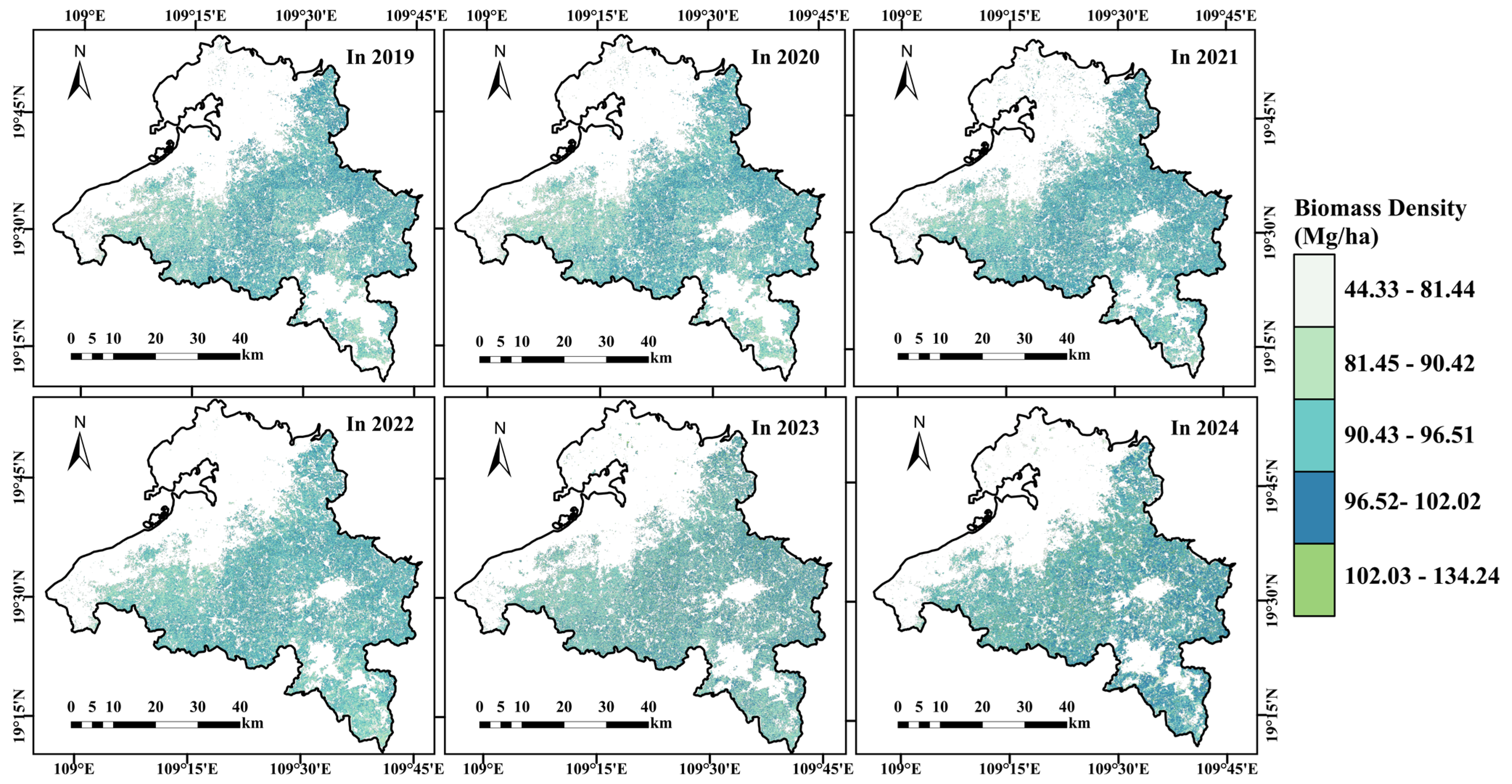
A biomass estimation model based on the RF algorithm was constructed to invert the biomass of rubber plantations in Danzhou City from 2019 to 2024. A biomass distribution map with a spatial resolution of 10 m was then generated (Figure 16), providing reliable data support for subsequent detailed studies.
The biomass of rubber plantations in Danzhou City was primarily concentrated in the 90–102 Mg/ha range, widely distributed throughout most of the city area, and generally showed a continuous distribution feature. The high biomass area (>102 Mg/ha) is primarily concentrated in the western and central-southern parts of the city, presenting a patchy or strip-like distribution. The low biomass area (<81 Mg/ha) is predominantly scattered along the forest edge or in fragmented areas. Overall, the spatial pattern of rubber plantation biomass in Danzhou City is relatively stable, with only specific local areas showing fluctuations.
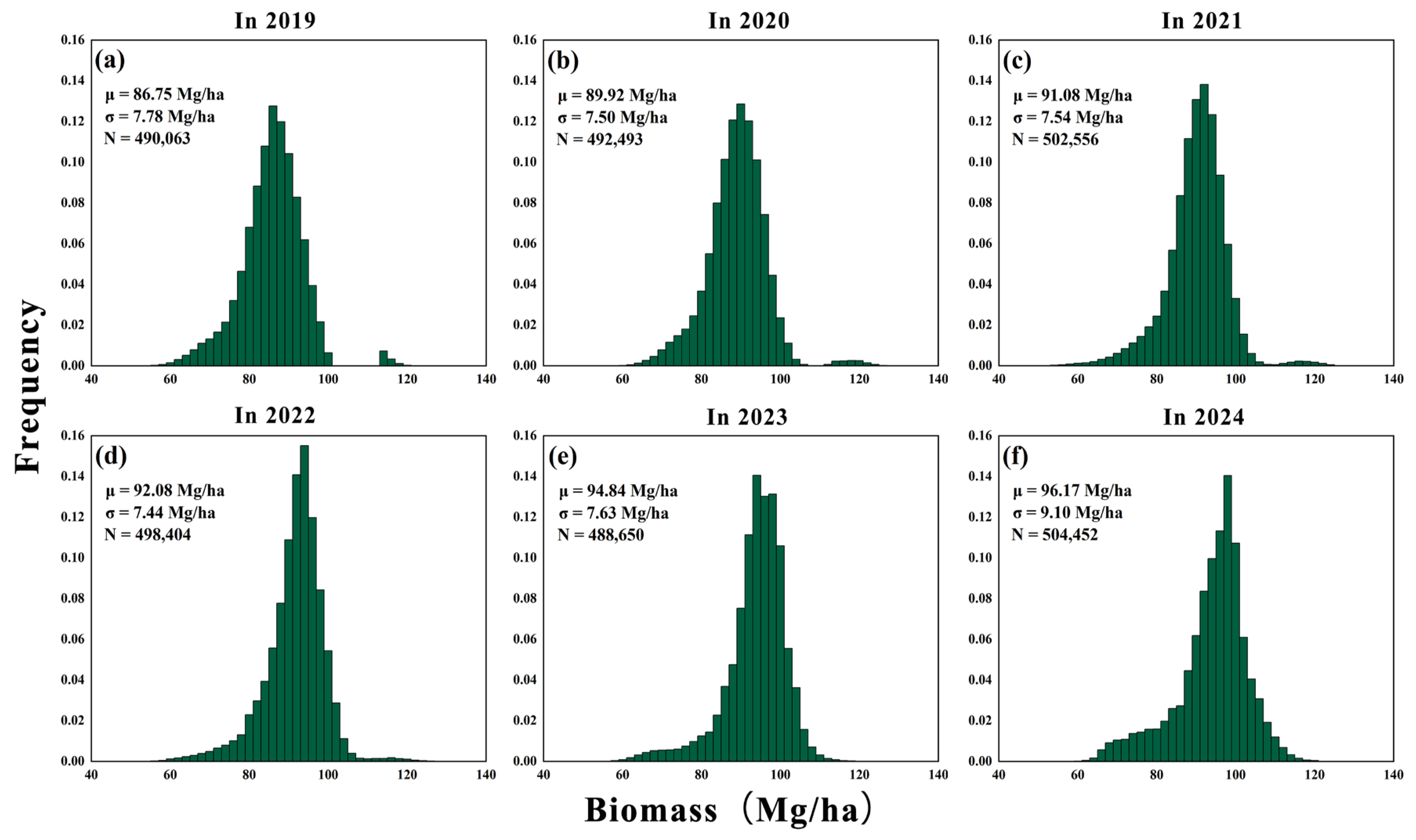
The biomass of the rubber plantations remained stable overall from 2019 to 2021, and the spatial pattern did not show any notable variation. Since 2022, the high biomass areas in some regions have contracted, while the low-to-medium biomass areas have slightly increased, showing a phased fluctuation in biomass density. From 2023 to 2024, the overall pattern once again became stable, with the high biomass areas still remaining in the core distribution area, but the range has been reduced compared with the previous period, indicating that although rubber plantations remain at a relatively high level overall, they are still affected by typhoon disasters, local human activities such as logging and conversion to other crops, and forest aging, presenting certain spatiotemporal heterogeneity. Furthermore, Figure 17 presents a histogram of the time series changes in rubber forest biomass from 2019 to 2024, clearly illustrating the variations and fluctuations in the biomass distribution across different years.
Further statistical analysis at the township scale (Table 12) reveals that the changes in rubber plantation biomass in each township are generally consistent with the overall trend of the city, but there are differences in specific levels and fluctuation amplitudes. For example, Ya Xing Town, Lan Yang Town, and Dong Cheng Town have maintained a high level for a long time, with strong stability; while Wan Xing Town, Guang Chun Town, and other places have experienced significant declines, reflecting the differentiated impacts of local natural conditions, management methods, and external disturbances in different regions. These results indicate that the superposition of macroscopic stability and township differences jointly shapes the spatiotemporal dynamic characteristics of rubber plantation biomass in Danzhou City.

4. Discussion

4.1. Advantages and Limitations of the RB_2020_KNDVI Model

The RB_2020_KNDVI model constructed in this study is a promising tool for identifying rubber plantations, offering advantages in terms of accuracy and vegetation index selection compared to previous methods. Chen et al. achieved a total accuracy of approximately 90% (Kappa = 0.86) in the Xishuangbanna region by combining multi-source phenological features with the RF algorithm [43]; Wang et al. achieved a precision of 91.25% (F1 = 0.932) using a multi-algorithm phenological integration framework [44]; Panboonyuen et al. proposed the deep learning model MeViT based on Landsat images, which classified rubber and various economic crops in Thailand as segmentation objects, achieving a precision of 92.22% and an F1 value of 93.44% [45]; Gao et al. used fused optical remote sensing data to draw a distribution map of rubber in Xishuangbanna, with the EVI index performing the best, and the overall accuracy in each year remained stable between 87% and 89.51% [46]. In this study, we focused on Danzhou City and constructed the RB_2020_KNDVI model. The KNDVI index effectively alleviated the saturation effect of traditional NDVI and EVI in high-vegetation coverage areas, significantly enhancing the distinction between rubber and non-rubber plantations. In the internal validation, the identification accuracy, recall rate, and F1 value of non-rubber plantations reached 0.95, and rubber plantations remained at a relatively high level of 0.92–0.93; in the external validation, the overall accuracy reached 91.63%, with a Kappa coefficient of 0.83, demonstrating overall performance superior to previous methods. Thus, the introduction of KNDVI and the good convergence of the model structure jointly contribute to the outstanding competitiveness of RB_2020_KNDVI in terms of accuracy, robustness, and generalization ability, providing solid support for rubber plantation monitoring at the regional scale.
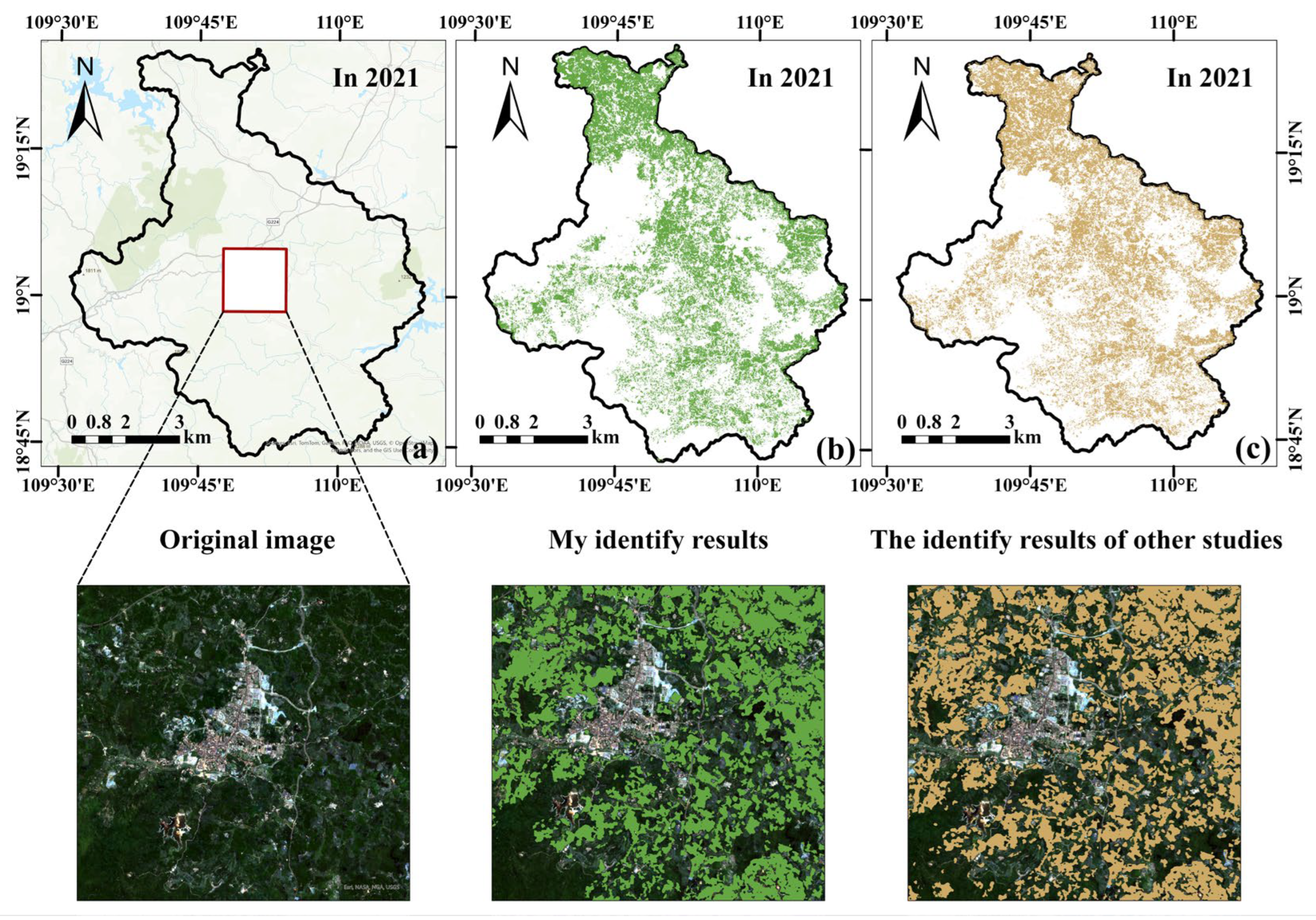
To further verify the adaptability of the RB_2020_KNDVI model in different regions, this study also applied the model to the identification task of rubber plantations in the Qiongzhong area in 2021. By selecting typical sample areas for testing, the results showed that the model also demonstrated high accuracy and stability in the Qiongzhong area (Figure 18). Although the terrain in Qiongzhong area is relatively complex and the climate conditions are different from those in Danzhou City, especially in the mountainous and diverse vegetation areas, the model still performed robustly and could well distinguish rubber plantations from non-rubber plantations. Choosing 2021 as the comparison year was because we referred to the research results of Wang et al. [47], which are highly authoritative. To ensure the fairness and consistency of the comparison, this study decided to also use the 2021 data for analysis, so as to more precisely compare the performance of the two models. By using the same year’s data, we can eliminate the potential influence of time differences, thereby more objectively evaluating the generalization ability and transferability of the model.
This study employed a deep learning model, while Wang et al. used the random forest algorithm; the differences in methods led to variations in the research background and application scenarios. Wang et al.’s research covered a large-scale Southeast Asian region and aimed to identify rubber plantations throughout the entire area, so their model could provide a relatively high overall accuracy. However, due to the extensive research area, the model’s performance in detailed and local regions might have been compromised. In contrast, this study focused on small-scale regions and was able to provide more detailed classification results in local areas. By comparing the images (Figure 18b,c), in terms of the clarity of the boundaries of the rubber plantations, the deep learning model in this study demonstrated strong discrimination capabilities in certain specific areas, especially in mountainous regions and transitional zones. It was able to accurately distinguish rubber plantations from non-rubber plantations and avoid misclassification. Overall, the research by Wang et al. has achieved outstanding results in large-scale applications, providing important references for the identification of rubber plantations. Its accuracy and contribution have a significant influence in this field. Meanwhile, the deep learning model in this study demonstrates unique advantages in the application potential of detailed areas, especially in complex terrains and diverse climatic conditions, where it can better capture details and provide more accurate classification results.
However, this study still has certain limitations. First, the model was primarily constructed and validated using samples from Danzhou City. Consequently, the adaptability of the model to a larger regional scope will require further verification. Second, while KNDVI is advantageous for the alleviation of saturation effects, its stability may be limited in complex terrains or extreme climate conditions. Finally, the potential impact of environmental factors (such as terrain undulation, soil moisture, and human interference) on classification accuracy has not yet been systematically evaluated. Future studies should optimize the model based on multi-source data fusion, multi-temporal analysis, and cross-regional transfer learning to enhance its application value on larger scales and more complex scenarios.

4.2. Comparative Analysis of Canopy Height and Biomass Estimation in Rubber Plantations Using Multi-Source Remote Sensing Data and Machine Learning Algorithms

ICESat-2 and GEDI laser radar data were integrated in this study to model canopy height in rubber plantations. The complementary nature of the two data sources in terms of spatial resolution and vertical structure effectively compensates for the shortcomings of a single data source in terms of spatial coverage, signal-to-noise ratio interference, and complex terrain conditions, resulting in higher reliability and robustness of the modeling results across different forest types [48]. In biomass modeling, historical data is further introduced to enhance the information support of the model, helping to improve the stability and interpretability of the estimation results. Based on this, this study systematically compares canopy height and biomass estimations using five machine learning algorithms (RF, BP, CNN, GBDT, and XGBoost).
This study used GEDI and ICESat-2 laser radar data to construct a canopy height model for rubber plantations. The XGBoost algorithm demonstrates high accuracy and stability in both internal and external validations, indicating that the selected data sources and methods have good applicability. Previous studies have focused on a single data source or algorithm optimization. For instance, Gao et al. improved the estimation accuracy based on GEDI data, combined with stand age and footprint-filtering techniques [49]; Potapov et al. generated global canopy height products by integrating GEDI and Landsat [50]; and Huang et al. improved the ATL08 algorithm using ICESat-2 photon point clouds, significantly improving the accuracy in mountainous environments [51]. Compared with these studies using a single data source, this paper integrates the complementary advantages of GEDI and ICESat-2 to ensure the reliability of accuracy while further enhancing the generalization ability of the model in regional-scale applications, providing a more robust technical path for rubber plantation carbon storage assessments and dynamic monitoring.
While the RF algorithm showed a relatively lower error level (RRMSE = 29.68%) in the internal validation stage, its coefficient of determination was only 0.60, and there was a systematic negative bias (bias = −0.21 m). Moreover, its accuracy in the external validation significantly decreased (R2 = 0.43, RRMSE = 11.19%), indicating that its generalization ability was insufficient. In contrast, the XGBoost algorithm achieved higher interpretability in the internal validation (R2 = 0.63), with a bias close to zero (0.01 m), and performed more robustly; in the external validation, its fitting effect was superior to that of the RF (R2 = 0.62, RRMSE = 6.82%), although there was a systematic underestimation (bias = −2.35 m). Its higher interpretability and lower relative error provided a guarantee for the application of the model in a larger spatial scale and more complex environments. Li et al. [52] developed an XGBoost model based on PlanetScope images, combining it with topographic factors, which significantly improved the accuracy of tree height prediction (R2 = 0.75, RMSE = 2.69 m). This highlighted the applicability and robustness of the method for canopy height modeling. Yu et al. [53] used high-resolution optical images obtained by drones and LiDAR DSM to compare the forest structure classification effects of RF, SVM, and XGBoost models. The XGBoost model performed best, achieving an F1 score of approximately 0.92 in both autumn and winter seasons, and further improved the classification performance in double-season images (from 0.68 to 0.92, an increase of 35.3%), highlighting the advantages and reliability of the XGBoost model in forest vertical structure modeling. Xu et al. [54] integrated multi-source data, including GEDI, AW3D30, and DEM, and compared the RF, BPNN, and XGBoost methods. The results showed that the XGBoost model performed the best in canopy height inversion and forest under terrain reconstruction, with a canopy height deviation of only −0.06 m, RMSE of 4.69 m, and forest under terrain RMSE of 9.82 m, fully demonstrating its ability to depict complex nonlinear relationships and its robustness in complex terrains. In summary, the XGBoost algorithm not only showed higher accuracy and robustness in this study but has also been verified by multiple studies to have superior performance in canopy height and forest structure modeling under various data sources and complex terrains, indicating that this algorithm is a reliable tool for canopy height estimation. Therefore, considering the comprehensive aspects of generalization ability, stability, and application value, XGBoost was determined to be the optimal model for estimating the canopy height of rubber plantations.
In the field of biomass remote sensing estimation, this study developed a model for estimating rubber plantation biomass using field survey data and historical records. The results showed that the RF model performed the best in estimating AGB. The BP and CNN models had weak fitting capabilities (with R2 values of 0.42 and 0.45, respectively), and the error levels were relatively high, making it difficult for them to meet application requirements. The GBDT model had a smaller bias (−1.33 Mg/ha), but its overall explanatory power was limited (with R2 = 0.51). In contrast, the XGBoost model performed slightly better than GBDT in terms of R2 (0.54) and RMSE (23.60 Mg/ha); however, its bias (4.9 Mg/ha) and relative bias (6.22%) were relatively high, indicating that specific systematic errors still existed. Comprehensive comparisons revealed that the RF model had the most balanced performance across all indicators. While it exhibited both high explanatory power (R2 = 0.72) and a low error level (RMSE = 16.04 Mg/ha, RRMSE = 21.48%, bias = 0.92Mg/ha), based on its comprehensive advantages in accuracy and stability, RF was ultimately selected as the optimal model for estimating rubber plantation biomass using remote sensing in this study.
Notably, this study’s modeling process incorporated historical sample data. Although this approach resulted in slightly lower model accuracy compared to some single-year studies, it is advantageous because it provides temporal constraints, which can better reflect the dynamic changes in rubber plantation biomass over multiple time periods and enhance the model’s generalization ability and application value. Compared with data from a single time point, data over multiple years help eliminate seasonal and accidental fluctuations, making the model more long-term adaptable and stable, and particularly suitable for assessing long-term ecological changes and biomass estimation at the regional scale. Furthermore, data spanning multiple years can offer greater representativeness, especially in regions with significant spatial heterogeneity. Although it may slightly affect accuracy, it can provide more comprehensive support for the model [55]. Some studies have further enhanced the accuracy and interpretability of biomass estimation by constructing biomass dynamic maps with higher temporal resolution and by combining historical data with modeling [56]. These studies have demonstrated the trend of integrating long-term monitoring data or historical data with remote sensing and other factors, highlighting the importance of multi-source data fusion in biomass modeling. This approach not only helps to build more comprehensive and stable biomass prediction models but also improves the reliability and applicability of the models, thereby providing more precise support for biomass estimation and comprehensively reflecting the complexity of forest ecosystems. Furthermore, these studies have verified the advantages of RFs from different perspectives. Fu et al. [57] used Sentinel-2 images to compare multiple algorithms and found that the RF model combined with Boruta optimization of variable combinations had the highest accuracy (R2 = 0.86, RMSE = 15.77 Mg/ha). Chen et al. [58] used the forest age maps generated by Landsat and Sentinel-2 to estimate biomass. The results showed that introducing forest age significantly improved the accuracy of the RF model (R2 = 0.82–0.96, RMSE = 4.08–10.59 Mg/ha), effectively alleviating the saturation problem. Ghosh et al. [59] combined Sentinel-1 SAR and Sentinel-2 vegetation indices and found that RF performed best when estimating the AGB of tropical forests (R2 = 0.71), outperforming parametric regression methods. Figure 19 presents the biomass regression results of this study based on the RF model, and marks the 95% confidence interval and 95% prediction interval. These intervals clearly show the range of variation in the model’s predicted values, presented together with the point estimates, thereby enhancing the transparency and reliability of the model’s predictions.
Although this study achieved relatively satisfactory results in modeling canopy height and biomass, it still has certain limitations. First, the ICESat-2 and GEDI laser radar data have deficiencies in terms of spatial coverage and observation quality; the former is significantly affected by noise in complex terrains, while the latter has sparse trajectories, making it difficult to achieve continuous observations, which may affect the estimation accuracy for local areas. Second, although the multi-year historical plot data introduced in the biomass modeling enhanced the explanatory power of the time dimension, its spatial distribution and observation conditions differed, resulting in slightly lower overall model accuracy compared to single-year studies. Third, although the machine learning model performed well in comparison, it still has systematic biases. For example, XGBoost underestimated external validations, and RF showed certain deviations in biomass estimation, indicating that the model’s robustness in complex environments or extreme conditions requires further verification. This study primarily relied on optical remote sensing, laser radar, and terrain factors, but did not fully consider potential driving factors, such as forest physiology, soil type, or management measures. Additionally, it did not involve more complex modeling frameworks, including deep learning. This may limit further improvement of accuracy. Finally, this study focused on the rubber plantations in Danzhou. The model’s generalizability in other regions or different forest types must be verified, and its application value for dynamic monitoring at a larger scale and higher temporal resolution needs to be explored.

4.3. Spatiotemporal Evolution and Biomass of Rubber Plantations in Danzhou City

From 2019 to 2024, the rubber plantation area in Danzhou City showed a fluctuating trend of “first increasing then decreasing”. In 2023, it reached a peak of 144,278.3 hectares, and in 2024, it slightly decreased to 138,068.5 hectares, remaining at a relatively high level overall. The rubber plantations are concentrated in the central, southeastern, and western areas of the city, forming a continuous and stable distribution pattern. Among them, Yaxing, Dacheng, and Nada Towns were the core planting areas, and Lanyang Town showed a continuous expansion trend. In contrast, coastal towns such as Dongcheng and Baimaijing experienced varying degrees of contraction. This spatial difference reflects the combined effects of regional natural conditions, management methods, and the intensity of human interference. The central and southeastern areas have gentle terrain, good drainage, and higher soil fertility, which are conducive to the concentrated and continuous growth of rubber trees. In contrast, the coastal and hilly areas are more prone to wind damage and terrain fragmentation, resulting in forest structures with relatively poor stability. It is worth noting that on 6 September 2024, Super Typhoon “Moeka” made landfall in Wenchang City, Hainan Province, causing severe damage to rubber plantations. According to the announcement of Hainan Natural Rubber Industry Group Co., Ltd. (Haikou, China), the company’s rubber plantations were scrapped for an area of approximately 230,000 mu (including cut trees and small seedlings), and this extreme climate event is the direct cause of a significant decline in the rubber plantation area in Danzhou City in 2024. This may explain the decrease in rubber plantation area after its peak in 2023.
The AGB of rubber plantations remained at a relatively high level (86–96 Mg/ha) even with the changes in area. The spatial distribution pattern was highly consistent with the area distribution: inland/hill areas such as Yaxing, Lan Yang, Dongcheng, and Dacheng Town had high value concentrations, whereas coastal towns like Guangcun and Baima Jing had low values. This spatial gradient has a clear ecological-management orientation: on the one hand, the inland and hilly areas have better soil development, superior water and fertilizer conditions, and are not in the main path of typhoons, which helps rubber trees form stable wood structures and continuous carbon accumulation. On the other hand, the coastal areas have been exposed to storm surges, salt fog, and frequent typhoon disturbances. The sandy soil has a poor water retention capacity, limiting the connectivity and stability of the forest stands, which results in lower productivity and biomass accumulation levels compared to inland areas [60]. It should be emphasized that “area-biomass consistency” is not equivalent to “stability”. Areas with high AGB often correspond to more mature/older forest stands, and such stands show higher vulnerability to strong winds, pests, diseases, and artificial regeneration.
The phased decline in biomass in 2022 and the stabilization in 2023–2024 indicate that the system may exhibit a “disturbance-recovery” dynamic rhythm. Multiple factors drive this fluctuation: (1) Extreme climate events, such as strong winds, which can cause branches to break, roots to loosen, or the deformation of the canopy structure, significantly reduce canopy density and the response of remote sensing signals in the short term [61]. Disturbances such as storms have been proven to significantly affect forest biomass and carbon storage. For instance, Gora et al. pointed out that storms are an important source of carbon loss in tropical forests, and this impact may persist for a long time after multiple storms, especially in rubber plantations, which are highly sensitive to wind speed and wind pressure [62]. Extreme climate events such as typhoons have a significant negative impact on their growth and biomass accumulation, and wind damage has also been confirmed by forest ecology research as one of the most significant disturbance mechanisms in tropical and subtropical forests. Rubber plantations have an extremely high sensitivity to wind speed and wind pressure [63]. Chen’s simulation study found that the strong winds of typhoons caused significant biomass loss in tropical artificial forests (including rubber plantations), especially in areas frequently affected by storms, where the volume of wood and carbon storage decreased significantly. These effects not only exacerbated the losses through direct wind damage (such as tree felling and loss of canopy), but also through indirect effects (such as soil erosion and water loss), further intensifying the losses [64,65]; (2) Succession of forest stand age structure: As the tree age increases, the rate of wood accumulation gradually slows down. The degradation of structural stability and wind resistance in mature forests intensifies their sensitivity to wind damage. Schwartz et al. [66] studied that mature forests suffered more severe wood loss after experiencing storms, and the recovery speed was slower. With the increase in tree age, the biomass loss caused by wind disasters becomes more persistent and may significantly affect the wood volume and carbon storage of forests in the long term.
Overall, the spatial pattern of the rubber plantation and its biomass in Danzhou shows strong coupling and stability. Areas with a large area often correspond with a larger biomass, indicating that the degree of forest stand continuity and the integrity of the canopy structure have a significant promoting effect on biomass accumulation. Consistent with the research results of Wang et al. and Ghosh et al. in tropical forests in Southeast Asia, this study reveals a stable pattern, indicating that the rubber plantation ecosystem in Hainan has gradually entered a mature, steady-state stage, and its carbon sink function is stable. Future research can further combine extreme climate events and dynamic changes in forest stand age structure to explore the ecological restoration process of rubber plantations and the elasticity of carbon storage, thereby providing a scientific basis for disaster prevention and mitigation, as well as the sustainable management of rubber plantations in tropical regions.

5. Conclusions

Sentinel-2 multi-rule remote sensing images and deep learning methods were used to systematically investigate the spatial patterns and dynamic evolution characteristics of rubber plantations in Danzhou City (2019–2024). ICESat-2 and GEDI laser radar data were also incorporated to construct a canopy height model, and biomass inversion was conducted using sample plots and drone point cloud data. The RB_2020_KNDVI model was the best at identifying rubber plantations, with a high overall accuracy and Kappa coefficient, effectively alleviating the saturation effect of traditional vegetation indices and improving the identification of rubber plantations. The XGBoost algorithm had the best fitting accuracy and robustness for in-canopy height modeling. The RF model had the best comprehensive performance for biomass estimation and was ultimately selected as the optimal model.
The results of this study provide technical support for spatiotemporal dynamic monitoring, forest carbon storage assessment, and tropical agricultural resource management in regional rubber plantations. New ideas regarding the accuracy and application value of remote sensing estimation are also presented. However, the model still has uncertainties in cross-regional and cross-period promotion because of the influence of sample plot size, data quality, and environmental differences, and the systematic deviation of the biomass model under different conditions must be further corrected. In the future, more abundant spatiotemporal samples can be introduced, combined with high-resolution drones and ground observations, and deep learning and transfer learning can be explored to improve the generalization ability and ecological interpretability of the model. This study provides data support for the sustainable operation of the Hainan rubber industry, carbon storage assessments, and ecological policy formulation.

Author Contributions

Conceptualization, Z.Q.; methodology, Y.C. and Z.Q.; software, Y.C.; vali-dation, Y.C., J.D., J.Q., Z.F., and Z.L.; formal analysis, Y.C., Z.Q., H.P., and P.G.; investigation, Y.C. and Z.L.; resources, Z.Q.; data curation, Y.C., J.Q., J.D., Z.L., and Z.F.; writing—original draft preparation, Y.C.; writing—review and editing, Y.C. and Z.Q.; visualization, Y.C. and J.D.; supervision, Z.Q.; project administration, Z.Q.; funding acquisition, Z.Q. All authors have read and agreed to the published version of the manuscript.

Funding

This research was funded by the National Natural Science Foundation of China, grant number 32160364.

Data Availability Statement

The data presented in this study are available on https://figshare.com/account/articles/30465212 (accessed on 9 December 2025).

Acknowledgments

The authors thank those students who assisted with fieldwork and data collection, as well as the instructors for their constructive comments on the improvement of this study.

Conflicts of Interest

The authors declare no conflicts of interest.

References

  1. Grogan, K.; Pflugmacher, D.; Hostert, P.; Mertz, O.; Fensholt, R. Unravelling the link between global rubber price and tropical deforestation in Cambodia. Nat. Plants 2019, 5, 47–53. [Google Scholar] [CrossRef]
  2. Golbon, R.; Cotter, M.; Sauerborn, J. Climate change impact assessment on the potential rubber cultivating area in the Greater Mekong Subregion. Environ. Res. Lett. 2018, 13, 084002. [Google Scholar] [CrossRef]
  3. Kusuma, Y.W.C.; Rembold, K.; Tjitrosoedirdjo, S.S.; Kreft, H. Tropical rainforest conversion and land use intensification reduce understorey plant phylogenetic diversity. J. Appl. Ecol. 2018, 55, 2216–2226. [Google Scholar] [CrossRef]
  4. Panda, B.K.; Sarkar, S. Environmental impact of rubber plantation: Ecological vs. economical perspectives. Asian J. Microbiol. Biotechnol. Environ. Sci. 2020, 22, 657–661. [Google Scholar]
  5. Lan, G.; Chen, B.; Yang, C.; Sun, R.; Wu, Z.; Zhang, X. Main drivers of plant diversity patterns of rubber plantations in the Greater Mekong sub-region. Biogeosciences Discuss. 2022, 19, 1995–2005. [Google Scholar] [CrossRef]
  6. Ahrends, A.; Hollingsworth, P.M.; Ziegler, A.D.; Fox, J.M.; Chen, H.; Su, Y.; Xu, J. Current trends of rubber plantation expansion may threaten biodiversity and livelihoods. Glob. Environ. Change 2015, 34, 48–58. [Google Scholar] [CrossRef]
  7. Wang, X.; Chen, B.; Dong, J.; Gao, Y.; Wang, G.; Lai, H.; Wu, Z.; Yang, C.; Kou, W.; Yun, T. Early identification of immature rubber plantations using Landsat and Sentinel satellite images. Int. J. Appl. Earth Obs. Geoinf. 2024, 133, 104097. [Google Scholar] [CrossRef]
  8. Chen, B.; Dong, J.; Hien, T.T.T.; Yun, T.; Kou, W.; Wu, Z.; Yang, C.; Wang, G.; Lai, H.; Liu, R. A full time series imagery and full cycle monitoring (FTSI-FCM) algorithm for tracking rubber plantation dynamics in the Vietnam from 1986 to 2022. ISPRS J. Photogramm. Remote Sens. 2025, 220, 377–394. [Google Scholar] [CrossRef]
  9. Azizan, F.; Astuti, I.; Young, A.; Aziz, A.A. Rubber leaf fall phenomenon linked to increased temperature. Agric. Ecosyst. Environ. 2023, 352, 108531. [Google Scholar] [CrossRef]
  10. Yusof, N.; Shafri, H.Z.M.; Shaharum, N.S.N. The use of Landsat-8 and Sentinel-2 imageries in detecting and mapping rubber trees. J. Rubber Res. 2021, 24, 121–135. [Google Scholar] [CrossRef]
  11. Xiao, C.; Li, P.; Feng, Z.; Liu, Y.; Zhang, X. Sentinel-2 red-edge spectral indices (RESI) suitability for mapping rubber boom in Luang Namtha Province, northern Lao PDR. Int. J. Appl. Earth Obs. Geoinf. 2020, 93, 102176. [Google Scholar] [CrossRef]
  12. Li, Y.; Liu, C.; Zhang, J.; Zhang, P.; Xue, Y. Monitoring spatial and temporal patterns of rubber plantation dynamics using time-series landsat images and google earth engine. IEEE J. Sel. Top. Appl. Earth Obs. Remote Sens. 2021, 14, 9450–9461. [Google Scholar] [CrossRef]
  13. Yang, J.; Xu, J.; Zhai, D.L. Integrating phenological and geographical information with artificial intelligence algorithm to map rubber plantations in Xishuangbanna. Remote Sens. 2021, 13, 2793. [Google Scholar] [CrossRef]
  14. Sun, Z.; Leinenkugel, P.; Guo, H.; Huang, C.; Kuenzer, C. Extracting distribution and expansion of rubber plantations from Landsat imagery using the C5. 0 decision tree method. J. Appl. Remote Sens. 2017, 11, 026011. [Google Scholar] [CrossRef]
  15. Abdullah, D.M.; Abdulazeez, A.M. Machine learning applications based on SVM classification a review. Qubahan Acad. J. 2021, 1, 81–90. [Google Scholar] [CrossRef]
  16. Liang, X.; Hyyppä, J.; Kaartinen, H.; Lehtomäki, M.; Pyörälä, J.; Pfeifer, N.; Holopainen, M.; Brolly, G.; Francesco, P.; Hackenberg, J. International benchmarking of terrestrial laser scanning approaches for forest inventories. ISPRS J. Photogramm. Remote Sens. 2018, 144, 137–179. [Google Scholar] [CrossRef]
  17. Wang, Y.; Lehtomäki, M.; Liang, X.; Pyörälä, J.; Kukko, A.; Jaakkola, A.; Liu, J.; Feng, Z.; Chen, R.; Hyyppä, J. Is field-measured tree height as reliable as believed–A comparison study of tree height estimates from field measurement, airborne laser scanning and terrestrial laser scanning in a boreal forest. ISPRS J. Photogramm. Remote Sens. 2019, 147, 132–145. [Google Scholar] [CrossRef]
  18. Pflugmacher, D.; Cohen, W.B.; Kennedy, R.E. Using Landsat-derived disturbance history (1972–2010) to predict current forest structure. Remote Sens. Environ. 2012, 122, 146–165. [Google Scholar] [CrossRef]
  19. Rodda, S.R.; Nidamanuri, R.R.; Fararoda, R.; Mayamanikandan, T.; Rajashekar, G. Evaluation of height metrics and above-ground biomass density from GEDI and ICESat-2 over Indian tropical dry forests using airborne liDAR data. J. Indian. Soc. Remote Sens. 2024, 52, 841–856. [Google Scholar] [CrossRef]
  20. Liu, X.; Su, Y.; Hu, T.; Yang, Q.; Liu, B.; Deng, Y.; Tang, H.; Tang, Z.; Fang, J.; Guo, Q. Neural network guided interpolation for mapping canopy height of China’s forests by integrating GEDI and ICESat-2 data. Remote Sens. Environ. 2022, 269, 112844. [Google Scholar] [CrossRef]
  21. Liang, Y.; Kou, W.; Lai, H.; Wang, J.; Wang, Q.; Xu, W.; Wang, H.; Lu, N. Improved estimation of aboveground biomass in rubber plantations by fusing spectral and textural information from UAV-based RGB imagery. Ecol. Indic. 2022, 142, 109286. [Google Scholar] [CrossRef]
  22. Navarro, A.; Young, M.; Allan, B.; Carnell, P.; Macreadie, P.; Ierodiaconou, D. The application of Unmanned Aerial Vehicles (UAVs) to estimate above-ground biomass of mangrove ecosystems. Remote Sens. Environ. 2020, 242, 111747. [Google Scholar] [CrossRef]
  23. Niu, Y.; Zhang, L.; Zhang, H.; Han, W.; Peng, X. Estimating above-ground biomass of maize using features derived from UAV-based RGB imagery. Remote Sens. 2019, 11, 1261. [Google Scholar] [CrossRef]
  24. Yang, S.; Xian, Y.; Tang, W.; Fang, M.; Song, B.; Hu, Q.; Wu, Z. Patterns and drivers of greenhouse gas emissions in a tropical rubber plantation from Hainan, Danzhou. Atmosphere 2024, 15, 1245. [Google Scholar] [CrossRef]
  25. Markus, T.; Neumann, T.; Martino, A.; Abdalati, W.; Brunt, K.; Csatho, B.; Farrell, S.; Fricker, H.; Gardner, A.; Harding, D. The Ice, Cloud, and land Elevation Satellite-2 (ICESat-2): Science requirements, concept, and implementation. Remote Sens. Environ. 2017, 190, 260–273. [Google Scholar] [CrossRef]
  26. Dorado-Roda, I.; Pascual, A.; Godinho, S.; Silva, C.A.; Botequim, B.; Rodríguez-Gonzálvez, P.; González-Ferreiro, E.; Guerra-Hernández, J. Assessing the accuracy of GEDI data for canopy height and aboveground biomass estimates in Mediterranean forests. Remote Sens. 2021, 13, 2279. [Google Scholar] [CrossRef]
  27. Huang, S.; Tang, L.; Hupy, J.P.; Wang, Y.; Shao, G. A commentary review on the use of normalized difference vegetation index (NDVI) in the era of popular remote sensing. J. For. Res. 2021, 32, 1–6. [Google Scholar] [CrossRef]
  28. Chandrasekar, K.; Sesha Sai, M.; Roy, P.; Dwevedi, R. Land Surface Water Index (LSWI) response to rainfall and NDVI using the MODIS Vegetation Index product. Int. J. Remote Sens. 2010, 31, 3987–4005. [Google Scholar] [CrossRef]
  29. Li, G.; Lai, H.; Chen, B.; Yin, X.; Kou, W.; Wu, Z.; Chen, Z.; Wang, G. Spatial Distribution Pattern of Forests in Yunnan Province in 2022: Analysis Based on Multi-Source Remote Sensing Data and Machine Learning. Remote Sens. 2025, 17, 1146. [Google Scholar] [CrossRef]
  30. Hu, L.; Li, W.; Xu, B. Monitoring mangrove forest change in China from 1990 to 2015 using Landsat-derived spectral-temporal variability metrics. Int. J. Appl. Earth Obs. Geoinf. 2018, 73, 88–98. [Google Scholar] [CrossRef]
  31. Liang, D.; Yang, F.; Zhang, T.; Yang, P. Understanding mixup training methods. IEEE Access 2018, 6, 58774–58783. [Google Scholar] [CrossRef]
  32. Foody, G.M. Explaining the unsuitability of the kappa coefficient in the assessment and comparison of the accuracy of thematic maps obtained by image classification. Remote Sens. Environ. 2020, 239, 111630. [Google Scholar] [CrossRef]
  33. Conger, A.J. Kappa and rater accuracy: Paradigms and parameters. Educ. Psychol. Meas. 2017, 77, 1019–1047. [Google Scholar] [CrossRef] [PubMed]
  34. Raffinetti, E. An extended study to measure dependence with grouped-ordinal variables generated by unobserved non-normal variables. Commun. Stat. Case Stud. Data Anal. Appl. 2020, 6, 448–472. [Google Scholar] [CrossRef]
  35. Kattenborn, T.; Leitloff, J.; Schiefer, F.; Hinz, S. Review on Convolutional Neural Networks (CNN) in vegetation remote sensing. ISPRS J. Photogramm. Remote Sens. 2021, 173, 24–49. [Google Scholar] [CrossRef]
  36. Neeraj, K.N.; Maurya, V. A review on machine learning (feature selection, classification and clustering) approaches of big data mining in different area of research. J. Crit. Rev. 2020, 7, 2610–2626. [Google Scholar]
  37. Li, J.; Cheng, J.-h.; Shi, J.-y.; Huang, F. Brief introduction of back propagation (BP) neural network algorithm and its improvement. In Advances in Computer Science and Information Engineering; Springer Nature: Berlin/Heidelberg, Germany, 2012; Volume 2, pp. 553–558. [Google Scholar]
  38. Kumar, M.; Agrawal, Y.; Adamala, S.; Pushpanjali; Subbarao, A.V.M.; Singh, V.K.; Srivastava, A. Generalization ability of bagging and boosting type deep learning models in evapotranspiration estimation. Water 2024, 16, 2233. [Google Scholar] [CrossRef]
  39. Shao, Z.; Ahmad, M.N.; Javed, A. Comparison of random forest and XGBoost classifiers using integrated optical and SAR features for mapping urban impervious surface. Remote Sens. 2024, 16, 665. [Google Scholar] [CrossRef]
  40. Gao, J. R-Squared (R2)–How much variation is explained? Res. Methods Med. Health Sci. 2024, 5, 104–109. [Google Scholar] [CrossRef]
  41. Roy, K.; Ambure, P.; Aher, R.B. How important is to detect systematic error in predictions and understand statistical applicability domain of QSAR models? Chemom. Intell. Lab. Syst. 2017, 162, 44–54. [Google Scholar] [CrossRef]
  42. Willmott, C.J.; Matsuura, K. Advantages of the mean absolute error (MAE) over the root mean square error (RMSE) in assessing average model performance. Clim. Res. 2005, 30, 79–82. [Google Scholar] [CrossRef]
  43. Chen, G.; Liu, Z.; Wen, Q.; Tan, R.; Wang, Y.; Zhao, J.; Feng, J. Identification of rubber plantations in southwestern China based on multi-source remote sensing data and phenology windows. Remote Sens. 2023, 15, 1228. [Google Scholar] [CrossRef]
  44. Wang, H.; Li, J.; Wang, J.; Deng, Y.; Gao, S.; Zou, J.; Chen, A.; Xu, H. A double-layer ensemble framework for rubber plantation mapping using multi-source data in the google earth engine: A case study of the southwestern border region of China. Int. J. Digit. Earth 2025, 18, 2520472. [Google Scholar] [CrossRef]
  45. Panboonyuen, T.; Charoenphon, C.; Satirapod, C. MeViT: A medium-resolution vision transformer for semantic segmentation on landsat satellite imagery for agriculture in Thailand. Remote Sens. 2023, 15, 5124. [Google Scholar] [CrossRef]
  46. Gao, S.; Liu, X.; Bo, Y.; Shi, Z.; Zhou, H. Rubber identification based on blended high spatio-temporal resolution optical remote sensing data: A case study in Xishuangbanna. Remote Sens. 2019, 11, 496. [Google Scholar] [CrossRef]
  47. Wang, Y.; Hollingsworth, P.M.; Zhai, D.; West, C.D.; Green, J.M.; Chen, H.; Hurni, K.; Su, Y.; Warren-Thomas, E.; Xu, J. High-resolution maps show that rubber causes substantial deforestation. Nature 2023, 623, 340–346. [Google Scholar] [CrossRef] [PubMed]
  48. Ling, Q.; Chen, Y.; Feng, Z.; Pei, H.; Wang, C.; Yin, Z.; Qiu, Z. Monitoring Canopy Height in the Hainan Tropical Rainforest Using Machine Learning and Multi-Modal Data Fusion. Remote Sens. 2025, 17, 966. [Google Scholar] [CrossRef]
  49. Gao, Y.; Yun, T.; Chen, B.; Lai, H.; Wang, X.; Wang, G.; Wang, X.; Wu, Z.; Kou, W. Improving the accuracy of canopy height mapping in rubber plantations based on stand age, multi-source satellite images, and random forest algorithm. Int. J. Appl. Earth Obs. Geoinf. 2024, 131, 103941. [Google Scholar] [CrossRef]
  50. Potapov, P.; Li, X.; Hernandez-Serna, A.; Tyukavina, A.; Hansen, M.C.; Kommareddy, A.; Pickens, A.; Turubanova, S.; Tang, H.; Silva, C.E. Mapping global forest canopy height through integration of GEDI and Landsat data. Remote Sens. Environ. 2021, 253, 112165. [Google Scholar] [CrossRef]
  51. Huang, X.; Cheng, F.; Wang, J.; Duan, P.; Wang, J. Forest canopy height extraction method based on ICESat-2/ATLAS data. IEEE Trans. Geosci. Remote Sens. 2023, 61, 5700814. [Google Scholar] [CrossRef]
  52. Li, Q.; Zhang, X.; Hao, D.; Yan, W.; Zhao, Q.; Tian, Y.; Zeng, Y. Mapping tree height in complex terrain of northern China using ultra-high-resolution images. Smart Agric. Technol. 2025, 12, 101338. [Google Scholar] [CrossRef]
  53. Yu, J.-W.; Yoon, Y.-W.; Baek, W.-K.; Jung, H.-S. Forest vertical structure mapping using two-seasonal optic images and LiDAR DSM acquired from UAV platform through random forest, XGBoost, and support vector machine approaches. Remote Sens. 2021, 13, 4282. [Google Scholar] [CrossRef]
  54. Xu, W.; Li, J.; Peng, D.; Wen, D. Reconstruction of understory terrain based on machine learning combined with GEDI and AW3D30 data. J. Mt. Sci. 2025, 22, 2159–2176. [Google Scholar] [CrossRef]
  55. May, P.B.; Finle, A.O. Spatial-temporal prediction of forest attributes using latent Gaussian models and inventory data. Arxiv Prepr. Arxiv 2025, 69, 100917. [Google Scholar] [CrossRef]
  56. Xu, W.; Jin, X.; Liu, J.; Yang, X.; Ren, J.; Zhou, Y. Analysis of spatio-temporal changes in forest biomass in China. J. For. Res. 2022, 33, 261–278. [Google Scholar] [CrossRef]
  57. Fu, Y.; Tan, H.; Kou, W.; Xu, W.; Wang, H.; Lu, N. Estimation of rubber plantation biomass based on variable optimization from Sentinel-2 remote sensing imagery. Forests 2024, 15, 900. [Google Scholar] [CrossRef]
  58. Chen, B.; Yun, T.; Ma, J.; Kou, W.; Li, H.; Yang, C.; Xiao, X.; Zhang, X.; Sun, R.; Xie, G. High-precision stand age data facilitate the estimation of rubber plantation biomass: A case study of Hainan Island, China. Remote Sens. 2020, 12, 3853. [Google Scholar] [CrossRef]
  59. Ghosh, S.M.; Behera, M.D. Aboveground biomass estimation using multi-sensor data synergy and machine learning algorithms in a dense tropical forest. Appl. Geogr. 2018, 96, 29–40. [Google Scholar] [CrossRef]
  60. Huang, Z.; Liu, Y.; Qiu, K.; López-Vicente, M.; Shen, W.; Wu, G.-L. Soil-water deficit in deep soil layers results from the planted forest in a semi-arid sandy land: Implications for sustainable agroforestry water management. Agric. Water Manag. 2021, 254, 106985. [Google Scholar] [CrossRef]
  61. Pugh, T.; Arneth, A.; Kautz, M.; Poulter, B.; Smith, B. Important role of forest disturbances in the global biomass turnover and carbon sinks. Nat. Geosci. 2019, 12, 730–735. [Google Scholar] [CrossRef] [PubMed]
  62. Gora, E.M.; McGregor, I.R.; Muller-Landau, H.C.; Burchfield, J.C.; Cushman, K.; Rubio, V.E.; Mori, G.B.; Sullivan, M.J.; Chmielewski, M.W.; Esquivel-Muelbert, A. Storms are an important driver of change in tropical forests. Ecol. Lett. 2025, 28, 70157. [Google Scholar] [CrossRef] [PubMed]
  63. Zhang, B.; Wang, X.; Yuan, X.; An, F.; Zhang, H.; Zhou, L.; Shi, J.; Yun, T. Simulating wind disturbances over rubber trees with phenotypic trait analysis using terrestrial laser scanning. Forests 2022, 13, 1298. [Google Scholar] [CrossRef]
  64. Chen, Y.; Huang, W.; Cheng, C.; Hong, J.; Yeh, F.; Luyssaert, S. Simulation of the impact of environmental disturbances on forest biomass in Taiwan. J. Geophys. Res. Biogeosci. 2022, 127, 6519. [Google Scholar] [CrossRef]
  65. Laurance, W.; Curran, T. Impacts of wind disturbance on fragmented tropical forests: A review and synthesis. Austral Ecol. 2008, 33, 399–408. [Google Scholar] [CrossRef]
  66. Schwartz, N.; Uriarte, M.; DeFries, R.; Bedka, K.; Fernandes, K.; Gutiérrez-Vélez, V.; Pinedo-Vasquez, M.A. Fragmentation increases wind disturbance impacts on forest structure and carbon stocks in a western Amazonian landscape. Ecol. Appl. 2017, 27, 1901–1915. [Google Scholar] [CrossRef] [PubMed]
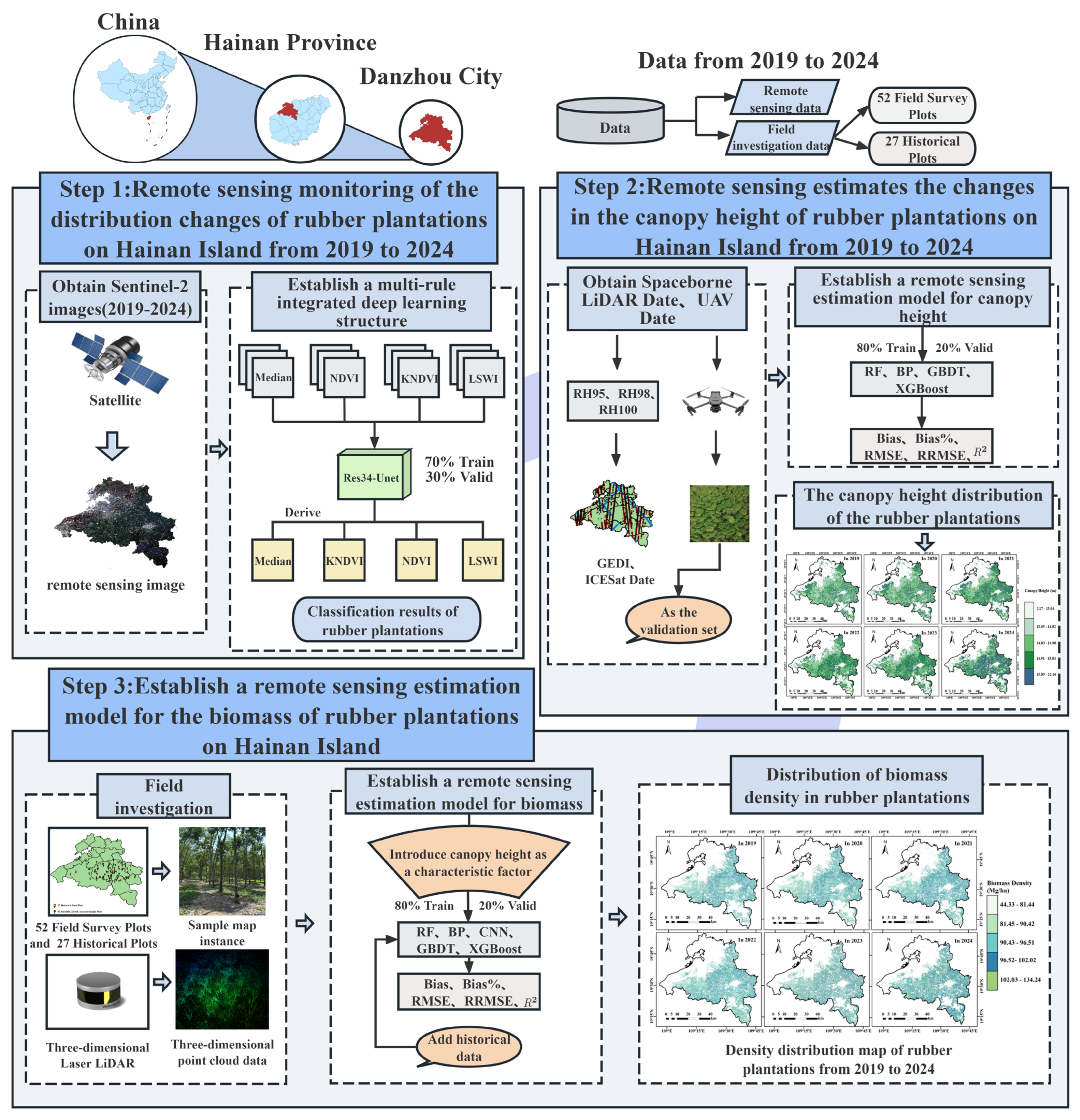
Figure 1. Technology roadmap.
Remotesensing 17 04042 g001
Figure 2. Schematic of the research area. (a) Hainan Island within China; (b) Danzhou City within Hainan Island; (c) Danzhou City with spatial LiDAR data points (ICESat-2 and GEDI) and field data points (52 LiDAR sample points and 27 historical data points). This figure is based on the WGS 1984 geographic coordinate system and the WGS 1984 UTM 49N-projected coordinate system.
Remotesensing 17 04042 g002
Figure 3. Details of the survey of sample areas.
Remotesensing 17 04042 g003
Figure 4. Network structure of ResNet34. F(X) refers to the residual of X, and X is the feature map that was output in the pervious convolution.
Remotesensing 17 04042 g004
Figure 5. Res34_Unet structure.
Remotesensing 17 04042 g005
Figure 6. Multi-rule integrated deep learning architecture.
Remotesensing 17 04042 g006
Figure 7. Four synthetic rules for remote sensing images. (a) Image generated by integrating with the NDVI index; (b) image generated by integrating with the LSWI index; (c) image generated by integrating with the KNDVI index; and (d) median synthesis image.
Remotesensing 17 04042 g007
Figure 8. Cross-entropy loss curve for RB_2020_KNDVI. The x-axis represents the number of training iterations.
Remotesensing 17 04042 g008
Figure 9. Typical rubber plantation identification results for Danzhou city from 2019 to 2024.
Remotesensing 17 04042 g009
Figure 10. Distribution map of rubber plantations in Danzhou city from 2019 to 2024.
Remotesensing 17 04042 g010
Figure 11. External validation results for four machine learning models used to predict the height of rubber forest canopies under RH95 conditions. The dark blue line represents the actual values and predicted values of the curve, and the light blue line represents the y = x reference line. (a) BP, (b) RF, (c) GBDT, and (d) XGBoost algorithms.
Remotesensing 17 04042 g011
Figure 12. External validation results for four machine learning models used to predict the height of rubber forest canopies under RH98 conditions. The dark blue line represents the actual values and predicted values of the curve, and the light blue line represents the y = x reference line. (a) BP, (b) RF, (c) GBDT, and (d) XGBoost algorithms.
Remotesensing 17 04042 g012
Figure 13. External validation results for four machine learning models used to predict the height of rubber forest canopies under RH100 conditions. The dark blue line represents the actual values and predicted values of the curve, and the light blue line represents the y = x reference line. (a) BP, (b) RF, (c) GBDT, and (d) XGBoost algorithms.
Remotesensing 17 04042 g013
Figure 14. Distribution map of rubber plantation canopy height in Danzhou city.
Remotesensing 17 04042 g014
Figure 15. Histogram of the canopy height of rubber plantations in Danzhou City from 2019 to 2024. μ and σ represent the average and standard deviation of the predicted tree canopy height of rubber plantations, while N indicates the total quantity.The histograms illustrate the distribution of canopy heights of rubber plantations in Danzhou City over six years (2019, 2020, 2021, 2022, 2023, and 2024), corresponding to subplots (af).
Remotesensing 17 04042 g015
Figure 16. Distribution map of rubber plantation biomass in Danzhou city.
Remotesensing 17 04042 g016
Figure 17. Histogram of the biomass of rubber plantations in Danzhou City from 2019 to 2024. μ and σ represent the average and standard deviation of the predicted biomass of rubber plantations, while N denotes the total number.The histograms illustrate the distribution of biomass of rubber plantations in Danzhou City over six years (2019, 2020, 2021, 2022, 2023, and 2024), corresponding to subplots (af).
Remotesensing 17 04042 g017
Figure 18. Comparison of rubber forest identification results in 2021. (a) The study area in Qiongzhong; (b) The rubber plantations results identified by the current research model; (c) The rubber plantations results identified by Wang et al.
Remotesensing 17 04042 g018
Figure 19. Uncertainty in Biomass Prediction of the RF Model.
Remotesensing 17 04042 g019
Table 1. Vegetation indices used in this study.
Feature CodeFeature NameFormula
KNDVIKernel Normalized Difference
Vegetation Index
tan ( ( ρ nir ρ red ) / ( ρ nir + ρ red ) 2 )
NDVINormalized Difference Vegetation Index ( ρ nir ρ red ) / ( ρ nir + ρ red )
LSWILand Surface Water Index ( ρ nir ρ swir ) / ( ρ nir + ρ swir )
Table 2. Parameter definitions for calculating internal validation metrics.
ParameterRepresentation Results
TPTrue Positive (predicted as positive and actually positive)
FPFalse Positive (predicted as positive, but actually negative)
TNTrue Negative (predicated as negative and actually negative)
FNFalse Negative (predicated as negative, but actually positive)
Table 3. Confusion matrix.
Confusion MatrixReference Data
Classified date Rubber plantationNon-rubber plantationTotal
Rubber plantationaba + b
Non-rubber plantationcdc + d
Totala + cb + da + b + c + d
Table 4. Remote sensing estimation model characteristics, factors of rubber plantations, canopy height, and biomass.
ModelFeature Factor
Canopy Height ModelHistorical Average Annual Temperature, Historical Average Annual Precipitation, Elevation, Slope, Aspect, EVI, GRVI, B1T3Mea, B1T5Mea, B3T3Hom
Biomass ModelCanopy Height, EVI, B9, B3T5Hom, B9T5Mea, B7T3Sem, B30T5Ent, B19T3Hom
EVI, enhanced vegetation index; GRVI, green-red vegetation index; B indicates spectral band variables, where B9 corresponds to the short-wave infrared 1 (SWIR-1) band; T, texture features; Mea, mean; Hom, homogeneity; Sem, semi-variance or second moment; and Ent, entropy.
Table 5. Internal evaluation results for four deep learning models.
Precision RecallF1 Score
Rubber
Plantation
Non-Rubber PlantationRubber
Plantation
Non-Rubber PlantationRubber
Plantation
Non-Rubber Plantation
RB_2020_KNDVI0.920.950.930.950.920.95
RB_2020_NDVI0.920.940.920.940.920.94
RB_2020_LSWI0.890.930.900.920.900.92
RB_2020_Median0.910.930.910.940.910.94
Table 6. Confusion matrix results.
Confusion MatrixReference Data
Classified date Rubber plantationNon-Rubber plantationTotal
Rubber plantation19802122192
Non-rubber plantation35543044659
Total233545166851
Table 7. External evaluation results of the RB_2020_KNDVI model.
Model Accuracy Result
RB_2020_KNDVICategoryProducer accuracyUser accuracyOverall accuracyKappa
Rubber plantation89.6390.18%91.63%0.83
Non-Rubber plantation93.0492.63%
Table 8. Distribution area of rubber plantations in each town (district) of Danzhou City (ha).
Town (District)\YearIn 2019In 2020In 2021In 2022In 2023In 2024
Baimajing Town17.0017.6324.5824.7210.0410.65
Dacheng Town22,799.1722,799.2922,193.6421,846.1922,688.2121,861.56
Dongcheng Town5531.815538.605405.675626.645772.665343.72
Eman Town98.4698.47129.9360.7675.89127.71
Guangcun Town5192.865192.864831.564361.924469.284325.74
Haotou Town1419.181502.841248.891254.711394.661218.54
HeqingTown17,313.5417,313.5516,546.8416,001.5017,109.8516,752.21
Lanyang Town16,139.7916,162.0517,502.4621,435.3121,528.9321,167.88
Mushang Town39.6386.90159.06109.6896.3593.09
NadaTown15,979.4015,999.3415,226.8215,118.6115,560.5215,163.07
Nanfeng Town9159.5510,281.9612,176.7113,844.7512,740.9311,919.28
Paipu Town642.35656.46556.31702.65694.75589.51
Wangwu Town1525.161559.111460.321378.771360.901155.29
XinzhouTown26.9028.0425.9834.5611.204.93
Yaxing Town38,919.5237,910.8037,194.4737,922.5940,650.0538,256.03
Zhonghe Town1.301.306.362.301.891.97
Yangpu Economic Development Zone30.8530.8470.9467.8386.9075.35
Danzhou City134,836.45135,180.01134,761.54139,801.49144,253.01138,109.81
Table 9. Four machine learning algorithms established internal accuracy verification of the canopy height model for the rubber plantations.
PercentilesModel
Algorithms
Training
Set R2
Testing Set
R2
Testing Set
Bias (m)
Testing Set
Relative
Bias (%)
Testing Set
RMSE (m)
Testing Set
RRMSE (%)
RH95RF0.790.61−0.16−1.473.6833.86
BP0.560.530.121.214.1342.28
GBDT0.780.62−0.04−0.423.6736.57
XGBoost0.760.60−0.20−2.013.6436.78
RH98RF0.780.61−0.19−1.633.7732.20
BP0.550.52−0.31−2.84.2939.30
GBDT0.790.60−0.41−3.673.8734.49
XGBoost0.760.61−0.07−0.643.8334.60
RH100RF0.780.60−0.21−1.643.7729.68
BP0.530.480.040.314.2735.85
GBDT0.780.610.09−0.803.7731.71
XGBoost0.740.630.010.133.6731.80
Table 10. External accuracy verification of canopy height models for rubber plantations established by four machine learning algorithms.
PercentilesModel
Algorithms
R2Bias
(m)
Relative Bias (%)RMSE
(m)
RRMSE
(%)
RH95RF0.352.6317.813.0020.29
BP0.21−1.28−8.662.2315.09
GBDT0.40−1.14−7.742.1414.48
XGBoost0.41−0.53−3.641.9913.47
RH98RF0.39−0.60−4.041.7712.00
BP0.26−2.33−15.752.6217.74
GBDT0.45−1.04−7.032.0013.55
XGBoost0.360.432.941.479.92
RH100RF0.43−0.28−1.891.6511.19
BP0.31−2.36−15.962.6217.77
GBDT0.401.9613.293.0620.73
XGBoost0.62−0.35−2.351.016.82
Table 11. Validation of the remote sensing estimation model for rubber forest biomass in Danzhou City.
Model
Algorithms
R2Bias
(Mg/ha)
Relative Bias
(%)
RMSE
(Mg/ha)
RRMSE
(%)
BP0.42−2.52−3.0531.1837.67
RF0.720.925.6116.0421.48
CNN0.453.885.4923.6733.54
GBDT0.51−1.33−1.9422.8733.45
XGBoost0.544.96.223.6029.85
Table 12. Rubber plantation biomass statistics for each town (district) of Danzhou city (Mg/ha).
Town (District)\YearIn 2019In 2020In 2021In 2022In 2023In 2024
Baimajing Town87.5990.3888.5688.8496.1381.46
Dacheng Town87.7091.1092.1493.8495.5695.88
Dongcheng Town87.3390.3290.9392.4194.5094.36
Eman Town83.0584.8789.0483.20103.3780.07
Guangcun Town88.9491.8892.8594.4896.7795.18
Haotou Town80.8682.9684.4487.1288.9686.81
HeqingTown88.3291.5592.7294.3296.1996.59
Lanyang Town86.1889.3390.7791.5094.2595.15
Mushang Town87.0589.0890.5889.24100.4883.01
NadaTown87.4490.7492.0393.6896.0396.35
Nanfeng Town85.9289.0690.4291.4594.5795.16
Paipu Town84.3386.7888.9790.6094.1089.87
Wangwu Town87.0189.7388.9091.9592.7590.11
XinzhouTown87.9190.4587.5686.2392.4279.62
Yaxing Town85.7088.7290.1392.0393.9494.32
Zhonghe Town86.0189.0580.6584.7596.6378.72
Yangpu Economic Development Zone76.2577.7789.1395.1898.2982.11
Danzhou City86.7589.9291.0892.0894.8496.17
Disclaimer/Publisher’s Note: The statements, opinions and data contained in all publications are solely those of the individual author(s) and contributor(s) and not of MDPI and/or the editor(s). MDPI and/or the editor(s) disclaim responsibility for any injury to people or property resulting from any ideas, methods, instructions or products referred to in the content.