A Semi-Automatic Framework for Dry Beach Extraction in Tailings Ponds Using Photogrammetry and Deep Learning

Highlights

What are the main findings?

• A semi-automated 3D framework is developed for extracting dry beach regions in tailings ponds, effectively capturing irregular boundaries and complex textures.
• DeepLabv3+ achieves superior segmentation accuracy and boundary continuity compared with SegNet and UNet.

What are the implications of the main findings?

• The demonstrated incremental training capability enables efficient model adaptation to challenging scenarios such as snow cover and strong shadows.
• The proposed method provides reliable 3D dry beach point clouds for accurate dry beach length measurement and morphological change monitoring.

Abstract

The spatial characteristics of the dry beach in tailings ponds are critical indicators for the safety assessment of tailings dams. This study presents a method for dry beach extraction that combines deep learning-based semantic segmentation with 3D reconstruction, overcoming the limitations of 2D methods in spatial analysis. The workflow includes four steps: (1) High-resolution 3D point clouds are reconstructed from UAV images, and the projection matrix of each image is derived to link 2D pixels with 3D points. (2) AlexNet and GoogLeNet are employed to extract image features and automatically select images containing the dry beach boundary. (3) A DeepLabv3+ network is trained on manually labeled samples to perform semantic segmentation of the dry beach, with a lightweight incremental training strategy for enhanced adaptability. (4) Boundary pixels are detected and back-projected into 3D space to generate consistent point cloud boundaries. The method was validated on two-phase UAV datasets from a tailings pond in Yunnan Province, China. In phase I, the model achieved high segmentation performance, with a mean Accuracy and IoU of approximately 0.95 and a BF of 0.8267. When applied to phase II without retraining, the model maintained stable performance on dam boundaries, while slight performance degradation was observed on hillside and water boundaries. The 3D back-projection converted 2D boundary pixels into 3D coordinates, enabling the extraction of dry beach point clouds and supporting reliable dry beach length monitoring and deposition morphology analysis.

1. Introduction

Tailings ponds are typically formed by valley interception or surrounding embankments and serve as primary storage sites for solid waste from mineral resource extraction. Their structural integrity is directly linked to the safety of downstream communities and the health of surrounding ecosystems [1,2,3,4]. With the increasing scale of mining operations and accumulation of tailings, effective stability monitoring and management of tailings ponds have become essential for geohazard prevention. The dry beach, which serves as the primary deposition zone, strongly influences pond stability. Its length determines the seepage line and provides a reliable indicator of dam safety [5,6,7]. Meanwhile, its slope gradient influences both the reservoir’s storage capacity and tailings deposition patterns [8,9,10]. Therefore, reliable delineation of the dry beach is necessary for comprehensive operational assessment and timely risk management. To enhance risk management, Chinese regulations have incorporated the dry beach length and slope into routine monitoring requirements.

Traditional measurement methods rely on manual field surveys, which involve visual observation [11], laser-based measurements [12], or ultrasonic level meters [13,14]. Although economical to implement, these methods are affected by operator experience, weather conditions, and site accessibility, often resulting in low accuracy and limited spatial coverage [15]. With the advancement of remote sensing and computer vision, Many scholars are conducting tailings pond monitoring based on images obtained from cameras or satellites [16,17,18]. 2D imaging methods, including K-means clustering [11], watershed algorithm [19], and edge detection [20], have been introduced for dry beach analysis. These techniques extract pixel coordinates at the waterline using visual features such as color, brightness, and texture and then convert them into geometric parameters with projection models. However, their performance heavily depends on threshold selection and remains sensitive to noise, illumination changes, and water surface reflections [21,22,23]. In recent years, semantic segmentation networks have shown strong performance in remote sensing image classification [24,25,26,27]. These networks can automatically extract multi-scale features from images and exhibit robustness in dealing with complex textures. They have been applied to beach–water segmentation tasks [28,29,30,31]. However, image-based approaches cannot capture 3D terrain features, which limits their application for morphological analysis, slope estimation, and 3D visualization.

In contrast to 2D images, point clouds serve as high-accuracy digital terrain models, offering a more comprehensive and precise representation of surface morphology [32,33]. Large-scale, high-resolution point clouds can be acquired either through LiDAR, including terrestrial laser scanning (TLS) and airborne laser scanning (ALS), or UAV photogrammetry. TLS can achieve very high geometric accuracy (millimeter-level), but covering extensive tailings pond areas requires deploying multiple scanning stations, which is labor-intensive [34] and may still leave portions of the area unmeasured. ALS offers broader coverage but has reduced accuracy (typically centimeter-level), comparable to that achievable by UAV photogrammetry [35,36]. UAV photogrammetry not only generates dense 3D point clouds but also provides high-resolution 2D images, which can be used for rapid semantic segmentation. Considering that dry beach changes generally occur at the meter scale, centimeter-level point cloud accuracy is sufficient for practical engineering applications, making UAV photogrammetry the preferred approach for tailings pond monitoring. However, the presence of complex surrounding features such as dams, hillslopes, and vegetation poses significant challenges for precise dry beach extraction from heterogeneous and large-scale point clouds. Common point cloud segmentation methods include region growing (RG) [37], random sample consensus (RANSAC) [38], density-based clustering [39], and deep learning approaches [40]. These techniques have demonstrated effectiveness in landslide detection [41,42], discontinuity extraction [43,44], and urban modeling [45,46,47]. Nevertheless, their applicability in dry beach identification still faces considerable challenges. First, the interface between dry beaches and the water body results in transitional areas characterized by low topographic contrast, rendering the identification of their boundaries difficult [30]. Second, the gently undulating and continuous surface morphology of dry beaches often leads to region-growing algorithms either incorrectly merging distinct areas or fragmenting homogeneous zones. While RANSAC is effective in extracting regular geometric features, it encounters limitations when handling complex morphological boundaries. Density-based clustering methods are also susceptible to variations in point density and occlusions, often leading to unstable extraction results [48,49]. Deep learning approaches offer strong feature learning capacities but require large labeled point cloud datasets [50], which are scarce and costly in tailings pond applications.

To overcome the limitations of existing 2D image methods in spatial quantification and the limitations of direct point cloud methods in robust semantic identification, this study develops a semi-automatic workflow for dry beach extraction in tailings ponds based on UAV photogrammetry and 3D reconstruction. The proposed framework establishes an integrated pipeline of “boundary image retrieval–semantic segmentation–3D back-projection–dry beach monitoring”. By utilizing the projection matrix derived from photogrammetric reconstruction, the 2D boundaries are accurately projected into 3D space, generating geometrically explicit and measurable 3D boundaries and corresponding dry beach point clouds. The strategy fully exploits the maturity and high accuracy of image-based deep learning and the spatial expressiveness of point clouds, while compensating for the inherent lack of spatial information in 2D methods and avoiding the high cost associated with direct point cloud deep learning. Such capabilities facilitate key applications in tailings pond management, including safety assessment of dams and monitoring of tailings deposition.

This paper is organized as follows. Section 2 details the overall workflow, including 3D reconstruction, dry beach boundary image retrieval, semantic segmentation, and 3D boundary extraction. Section 3 validates the reliability and accuracy of the method using two phases of UAV images. Section 4 discusses the generalization capability, advantages, along with practical engineering applications. Section 5 concludes the study and outlines directions for future work.

2. Method

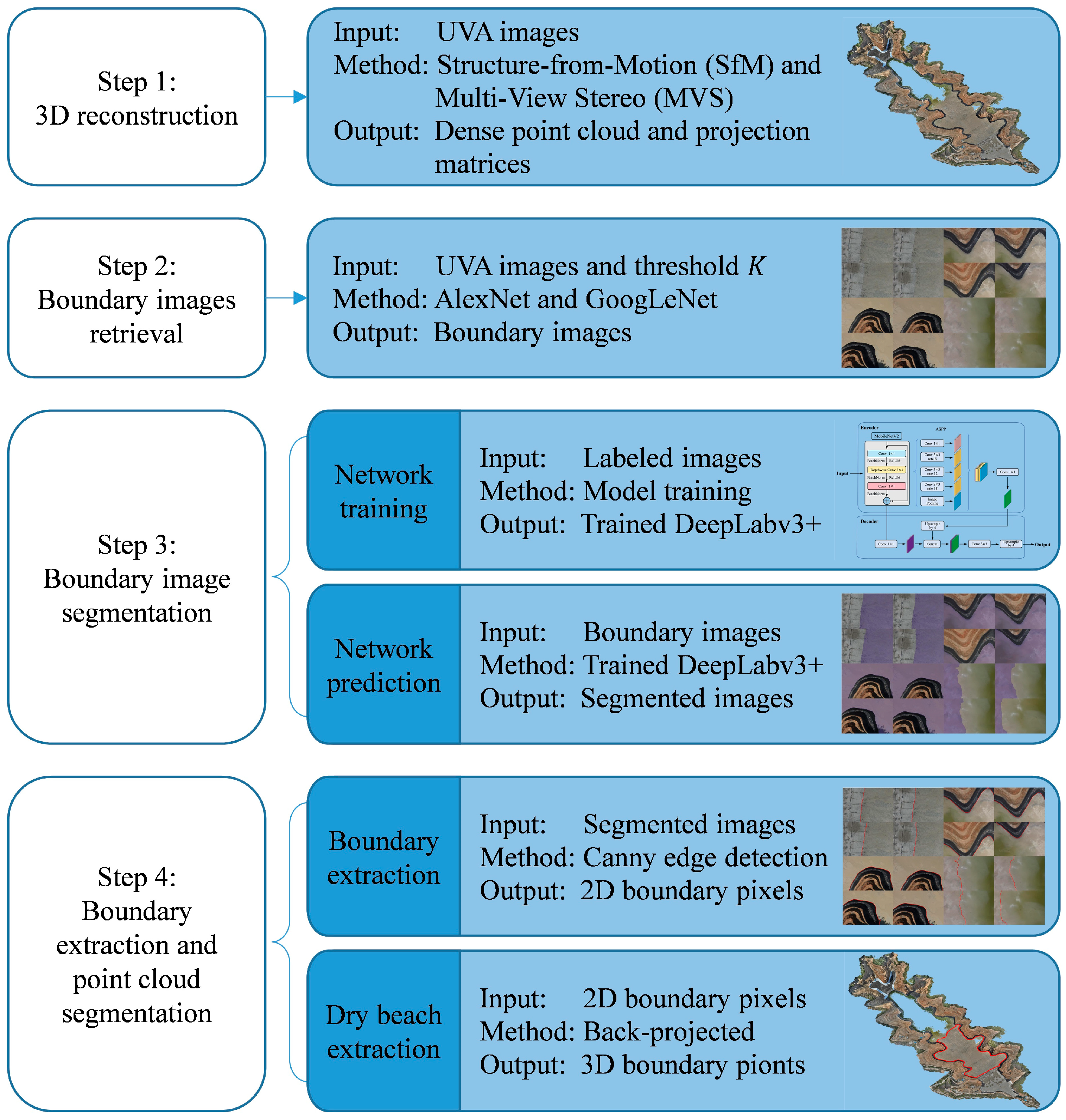
The proposed method comprises four main steps (Figure 1): (1) 3D reconstruction. UAV images are automatically processed to generate a dense point cloud, and projection matrices are obtained to link 2D pixels with 3D points. (2) Boundary image retrieval. Image features are automatically extracted using AlexNet [51] and GoogLeNet [52]. Representative boundary images are manually selected. Images containing dry beach boundaries are then automatically retrieved based on similarity. (3) Boundary image segmentation. The retrieved images are automatically segmented with DeepLabv3+ [53] trained by manually labeled images to delineate the dry beach regions at the pixel level. (4) Boundary extraction and point cloud segmentation. Dry beach boundaries are subsequently automatically extracted and back-projected into 3D space to extract the corresponding dry beach point cloud.

2.1. 3D Reconstruction

To achieve 3D identification of the dry beach in the tailings pond, aerial images captured by UAVs are first processed through Structure-from-Motion (SfM) and Multi-View Stereo (MVS) algorithm to generate a dense point cloud. Simultaneously, a projection matrix is calculated for each image, which records the camera pose in the 3D coordinate system. These matrices allow 2D boundary pixels to be transformed into 3D coordinates. The 3D reconstruction process mainly involves the following steps:

(1) Feature matching and fundamental matrix estimation.

Feature points and their local descriptors are extracted from all images using feature extraction algorithms such as Scale Invariant Feature Transform (SIFT) [54]. Initial correspondences between two images are established by matching similar feature points. Let p₁ = [u₁, v₁, 1], p₂ = [u₂, v₂, 1] denote normalized pixel coordinates in two images, respectively. These coordinates satisfy the constraint defined by the fundamental matrix F:

$${p_2}^{\mathrm{T}}F{p}_1=0$$

(1)

$$F={K_2}^{-\mathrm{T}}[t_{\times }]R{K_1}^{-1}$$

(2)

Here, the rotation matrix R and translation vector t represent the relative pose between the cameras corresponding to the two images. K₁, K₂ denote the intrinsic parameter matrix of their respective cameras, and [t_x] is the skew-symmetric matrix of t. The fundamental matrix F is estimated using at least eight pairs of matched feature points. Given the intrinsic parameters, the essential matrix E related to the fundamental matrix F is defined as follows:

$$E={K_2}^{\mathrm{T}}F{K}_1=[t_{\times }]R$$

(3)

By performing singular value decomposition (SVD) on E, the rotation matrix R and translation vector t between the two cameras can be determined.

(2) Camera poses estimation and triangulation.

The first camera is fixed as the world coordinate frame (R₁ = I, t₁ = 0), and the pose of the second camera (R₂, t₂) is recovered from the essential matrix E, as described above. Triangulation is then performed for matched points between the first two images to calculate their 3D coordinates X_j. Starting from the third image, the camera poses (R_i, t_i) of subsequent images are determined by solving the Perspective-n-Point (PnP) problem. Specifically, given a set of known 3D points X_j and their corresponding pixel coordinates p_ij in image I_i, along with the camera intrinsics K_i, the camera poses (R_i, t_i) can be estimated, as expressed in Equation (4).

$$p_{ij}~K_i[R_i|t_i]X_j$$

(4)

By iteratively processing all images, the projection matrix K_i [R_i|t_i] for each image and the corresponding sparse point cloud are obtained.

(3) Bundle adjustment

To correct errors in the initial estimates of camera poses and 3D point coordinates, bundle adjustment is applied to optimize all camera poses and 3D points by minimizing the overall reprojection error across all images. Specifically, the reprojection error is defined as the difference between the observed 2D pixel coordinates p_ij and the projected coordinates of the corresponding 3D points, as shown in Equation (5).

$$\underset{R_i,t_i,X_j}{\min }{\displaystyle \sum _{i,j}‖p_{ij}-proj(K_i,R_i,t_i,X_j)‖}$$

(5)

Through nonlinear least squares optimization, both camera poses and 3D points are simultaneously adjusted, resulting in a more accurate sparse point cloud.

(4) Dense point cloud construction

Dense point clouds are generated using the Multi-View Stereo (MVS) algorithm [55]. Given a pixel p_ij in an image, a 3D ray is defined by its corresponding projection matrix:

$$X(d)={R_i}^{\mathrm{T}}(d{K_i}^{-1}{p}_{ij}-t_i)$$

(6)

where d represents the depth to be estimated, and X(d) denotes the 3D coordinate of the pixel p_ij at depth d. The MVS algorithm evaluates the consistency of p_ij across multiple views at varying depths and selects the depth that achieves the best overall consistency with all observations as its 3D coordinate.

This process reconstructs a dense point cloud and determines the corresponding projection matrix for each image. These projection matrices define the relationship between 2D pixels and 3D coordinates, enabling the transfer of semantic information from images to the point cloud.

2.2. Boundary Image Retrieval

The dry beach in tailings ponds exhibits three distinct geomorphic interfaces: (1) the dry beach–dam, (2) the dry beach–hillside, and (3) the dry beach–reservoir water, as illustrated in Figure 2. Retrieving images containing these boundaries from a large UAV dataset is a challenging task, as manual inspection of thousands of images is time-consuming and susceptible to errors. To address this issue, the pretrained AlexNet and GoogLeNet models, both trained on the ImageNet dataset [56], are employed for feature extraction. Boundary images are then retrieved semi-automatically based on a weighted combination of cosine distances calculated from features extracted by both networks.

2.2.1. Image Feature Extraction

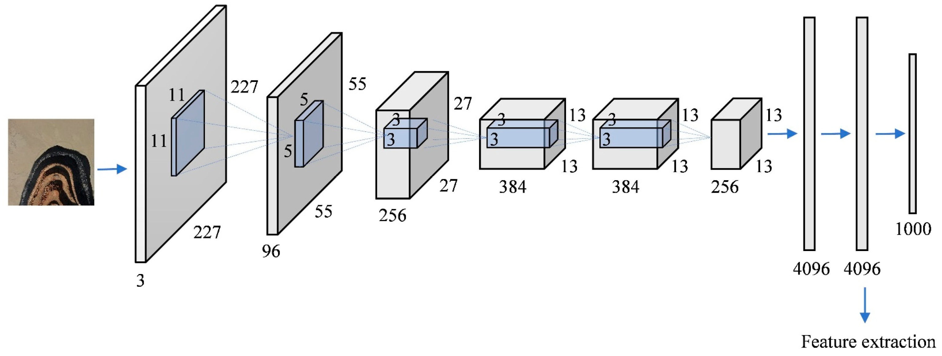
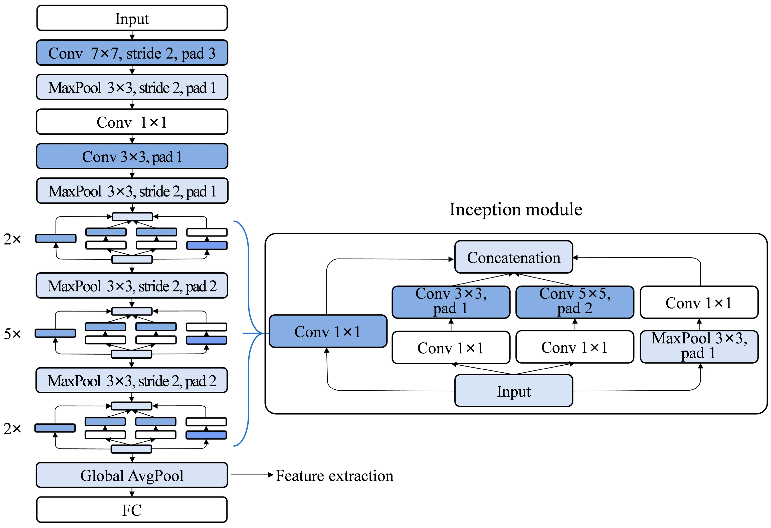
The architecture of AlexNet consists of an input layer, five convolutional layers, and three fully connected layers (Figure 3). All input images are standardized to 227 × 227 pixels before processing. In this study, the feature is extracted from the second fully connected layer, generating 4096-dimensional feature vectors. This layer captures high-level semantic information while preserving some spatial structural details. GoogLeNet, as shown in Figure 4, comprises nine Inception modules. Each module integrates 1 × 1, 3 × 3, and 5 × 5 convolutions with 3 × 3 max pooling to increase the network width and enhance multi-scale feature extraction capability [52]. In this work, the global average pooling layer is chosen as the output feature layer, generating 1024-dimensional feature vectors. Located at the end of the backbone, this layer aggregates multi-scale convolutional responses, enabling comprehensive capture of both spatial structure and semantic characteristics. To comply with the architectural requirements of GoogLeNet, input images are standardized to 224 × 224 pixels.

For each image, deep features are extracted using AlexNet and GoogLeNet. Specifically, each image is represented by two feature vectors: (1) a 4096-dimensional feature vector $f^A\in {ℝ}^{4096}$ extracted from the AlexNet, and (2) a 1024-dimensional feature vector $f^G\in {ℝ}^{1024}$ extracted from the GoogLeNet. These two feature vectors jointly describe the visual characteristics of the input image.

2.2.2. Image Feature Similarity Calculation

To quantify the similarity between two images, the cosine distance is adopted to measure the distance between their corresponding feature vectors. Given two images i and j, their cosine distance of AlexNe features and GoogLeNe features are, respectively, defined as:

$$d_A(i,j)=1-{\displaystyle \frac{f_i^A\cdot f_j^A}{‖f_i^A‖\times ‖f_j^A‖}}$$

(7)

$$d_G(i,j)=1-{\displaystyle \frac{f_i^G\cdot f_j^G}{‖f_i^G‖\times ‖f_j^G‖}}$$

(8)

where ${\mathbf{f}}_i^A$ and ${\mathbf{f}}_j^A$ denote the AlexNet features of images i and j, respectively, and ${\mathbf{f}}_i^G$ and ${\mathbf{f}}_j^G$ denote the corresponding GoogLeNet features. A smaller cosine distance indicates a higher similarity between the two images.

To avoid relying on a single network for similarity evaluation, a weighted fusion strategy is adopted to combine the two distances:

$$d(i,j)=r\cdot d_A(i,j)+\left(1-r\right)\cdot d_A(i,j)$$

(9)

where d(i,j) represents the similarity between images i and j and ranges from 0 to 1, with 0 indicating high similarity and 1 indicating high dissimilarity. r $\in$ [0, 1] is a weighting factor controlling the relative contribution of the two networks.

For boundary image retrieval, a small set of n representative boundary images is manually selected as reference templates. For each candidate image in the UAV dataset, the similarity d(i,j) is calculated with respect to each template image. To automatically identify boundary images, a similarity threshold K is applied: candidate images with d(i,j) < K are classified as boundary images, while those with d(i,j) > K are discarded (Equation (10)). The similarity threshold K was determined by examining the retrieval results to ensure high retrieval precision of boundary images. Specifically, K is chosen such that candidate images with similarity below K are very likely to correspond to boundary images, while minimizing the inclusion of non-boundary images.

$$\underset{i=1,\dots ,n}{\min }d(i,j)<K\Rightarrow \mathrm{image}j\mathrm{is}\mathrm{identified}\mathrm{as}\mathrm{a}\mathrm{boundary}\mathrm{image}$$

(10)

2.3. Boundary Image Segmentation

The dry beach in tailings ponds exhibits distinct geomorphological features, making it visually distinguishable from its surroundings. To extract dry beach boundaries, this study employs the DeepLabv3+ semantic segmentation network. Built on an encoder–decoder architecture, DeepLabv3+ captures high-level semantic information while preserving fine details, making it particularly suited for blurred or complex boundaries [53].

2.3.1. Network Architecture

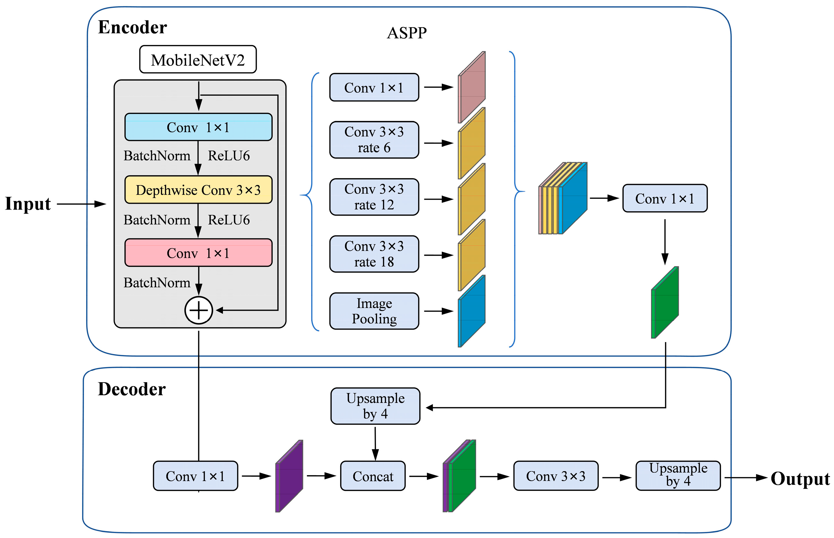
To balance segmentation accuracy and computational efficiency, the standard Xception [57] backbone of DeepLabv3+ is replaced with MobileNetV2 in this study. Although MobileNetV2 achieves slightly lower classification accuracy than Xception, it significantly reduces computational cost and model parameters, effectively decreasing network complexity and maintaining strong image structural perception [58]. The modified architecture (Figure 5) retains the core components of DeepLabv3+, including the Atrous Spatial Pyramid Pooling (ASPP) module with dilation rates of 6, 12, and 18 for multi-scale context aggregation, and the decoder structure for boundary refinement through feature fusion. The processing pipeline includes feature extraction by MobileNetV2, multi-scale context aggregation by the ASPP module, and upsampling with detail restoration by the decoder. The network ultimately outputs a pixel-level segmentation map distinguishing “dry beach” from “background” with the output size matching the input image.

2.3.2. Network Training

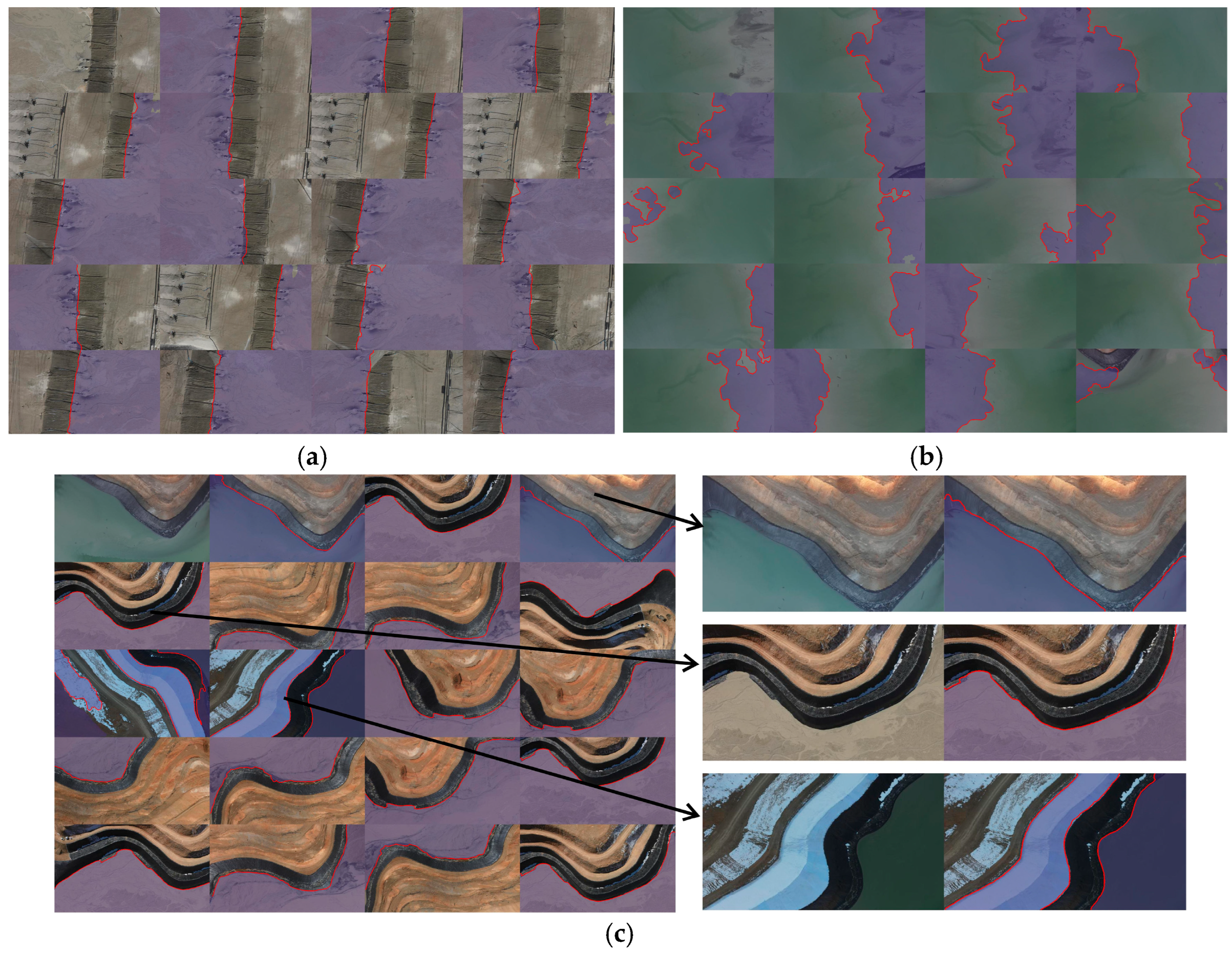
Due to the absence of available labeled datasets for dry beach boundary segmentation in tailings ponds, we manually constructed a labeled dataset. A total of 140 representative images were selected from the initial retrieved UAV images, comprising 30 dam-beach, 60 hillside-beach, and 50 water-beach cases. The selection was based on criteria of representativeness, boundary clarity, and structural integrity, ensuring dataset comprehensiveness and model generalization. The dataset was partitioned into training (120 images) and validation (20 images) sets.

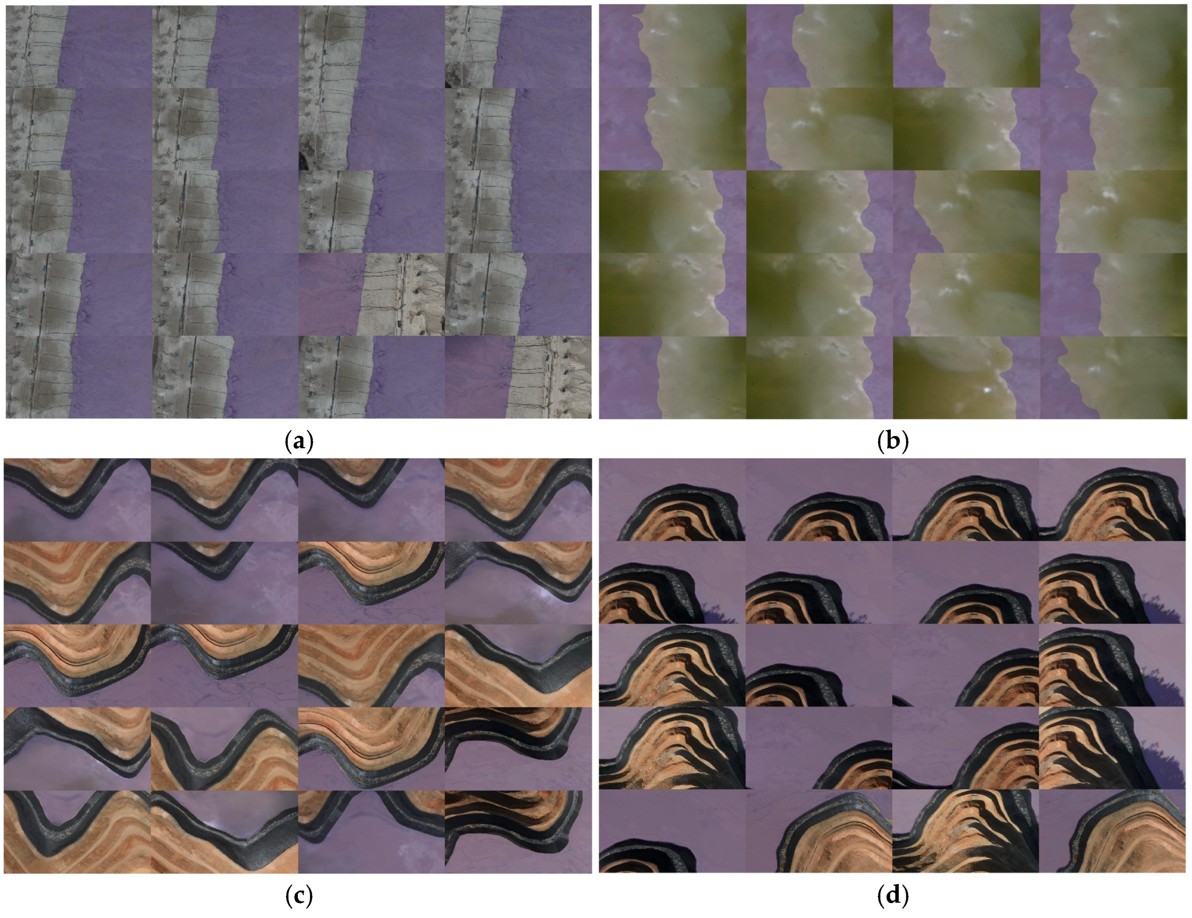
The original images were standardized to 395 × 700 pixels to meet the network input requirements while reducing memory consumption and improving training efficiency. Annotations followed a strict protocol: dry beach regions were labeled with purple masks (dry beach), while regions outside the dry beach, including tailings dam, hillside, and water, were labeled with green masks (background). Examples of the annotated masks for the three boundary types are shown in Figure 6.

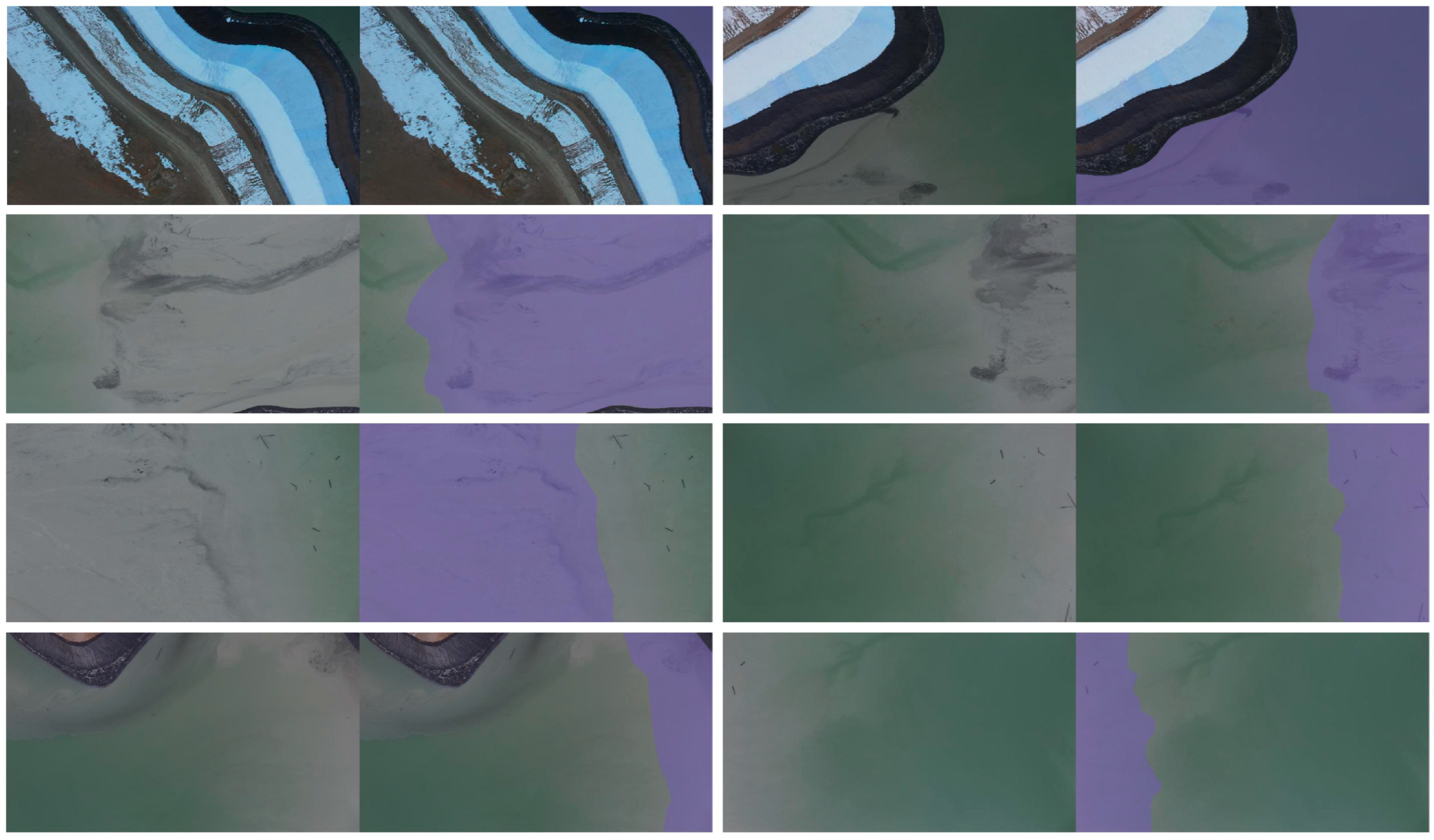
Data augmentation was applied to enhance the model’s robustness against illumination variations, viewpoint changes, and boundary ambiguities. First, each training image underwent four random brightness and contrast adjustments, generating five variants (including the original). Each variant was then rotated by 90°, 180°, 270°, and horizontally flipped, which generated 25 augmented samples per original image. All geometric transformations were simultaneously applied to the corresponding pixel-level labels to maintain spatial correspondence. The augmented images and labels were resized to the original resolution to ensure pixel alignment. 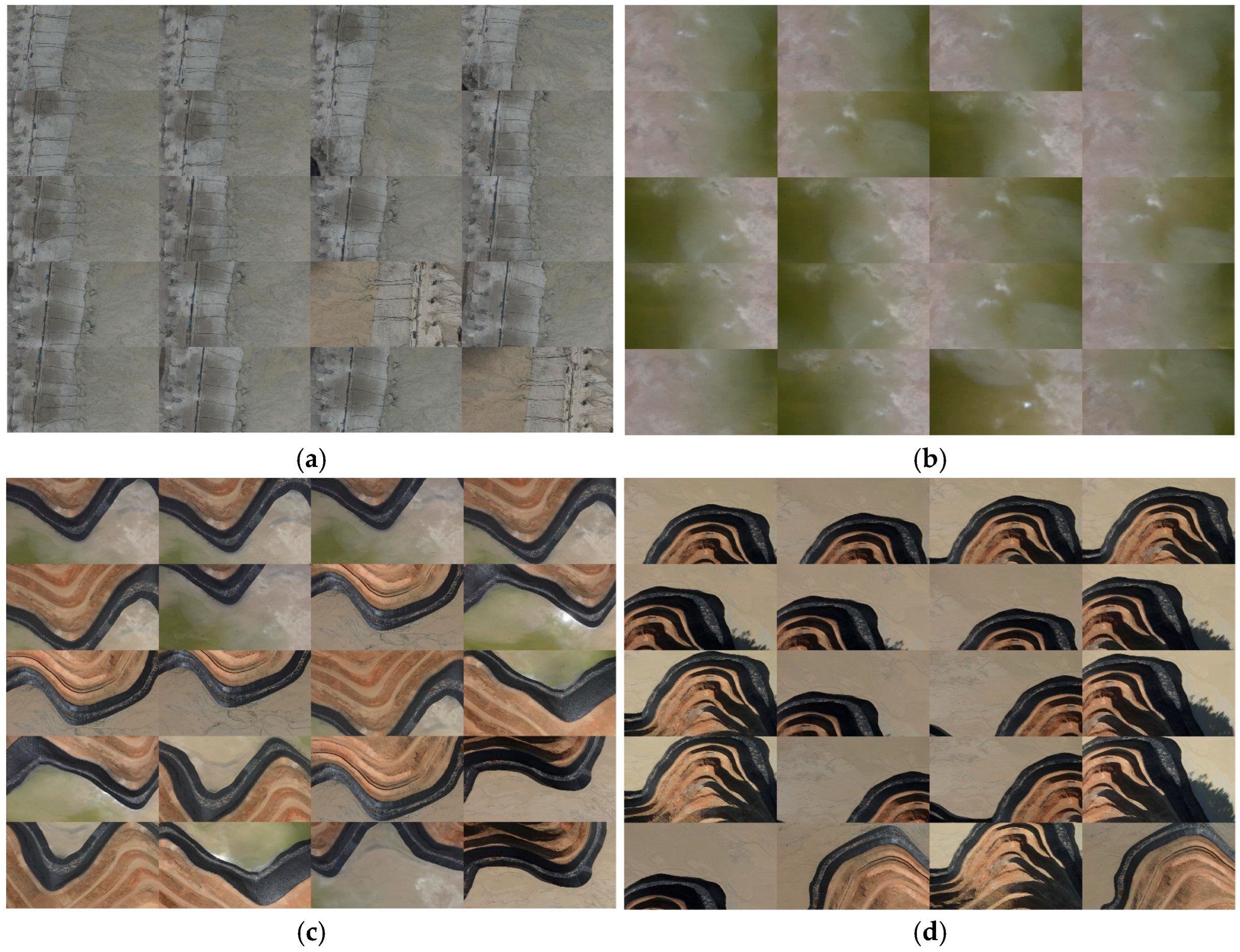Figure 7 illustrates a typical example of the augmented examples, showing the preservation of boundary structures and increased sample diversity.

In this study, the DeepLabv3+ model was trained on a desktop equipped with an Intel Core i5-12600KF CPU, 32 GB RAM, and an NVIDIA RTX 3060Ti GPU. The training parameters were set with a mini-batch size of 8, a maximum of 50 epochs, and an initial learning rate of 0.001, and the Adam optimizer was employed with adaptive learning rate adjustment. Upon convergence, the trained model was applied to segment all retrieved dry beach boundary images.

2.3.3. Lightweight Incremental Training Strategy

To mitigate performance degradation caused by variations in environmental conditions across different acquisition phases, a lightweight incremental training strategy is introduced to enhance the generalization capability of the segmentation model with a small additional labeling cost.

This strategy assumes that the segmentation network has been pre-trained using an initial annotated dataset. Specifically, the baseline DeepLabv3+ model is first trained on the annotated images from initial acquisition (referred to as ‘phase I’ in Section 3.1), as described in Section 2.3.2. When the trained model is applied to newly acquired imagery and performance degradation is observed in certain boundary types, a small number of representative samples from the new phase dataset are selectively chosen for incremental annotation. These samples are preferentially selected from regions exhibiting significant missegmentation, such as areas affected by strong illumination changes, surface cover transitions, or complex reflection conditions.

The newly annotated samples are then merged with the existing training dataset to construct an updated training set. To compensate for the limited number of incremental samples, data augmentation techniques (rotation, flipping, and brightness and contrast adjustments) are applied to enrich feature diversity and reduce the risk of overfitting. Instead of retraining the network from scratch, the pre-trained model is subsequently fine-tuned using this combined dataset, enabling the network to retain previously learned structural features while adapting to the newly introduced appearance variations.

This lightweight incremental training strategy allows efficient cross-phase adaptation with low annotation effort and computational cost, while maintaining the overall efficiency and practical applicability. It provides a viable solution for long-term dry beach monitoring under continuously evolving environmental conditions.

2.4. Boundary Extraction and Point Cloud Segmentation

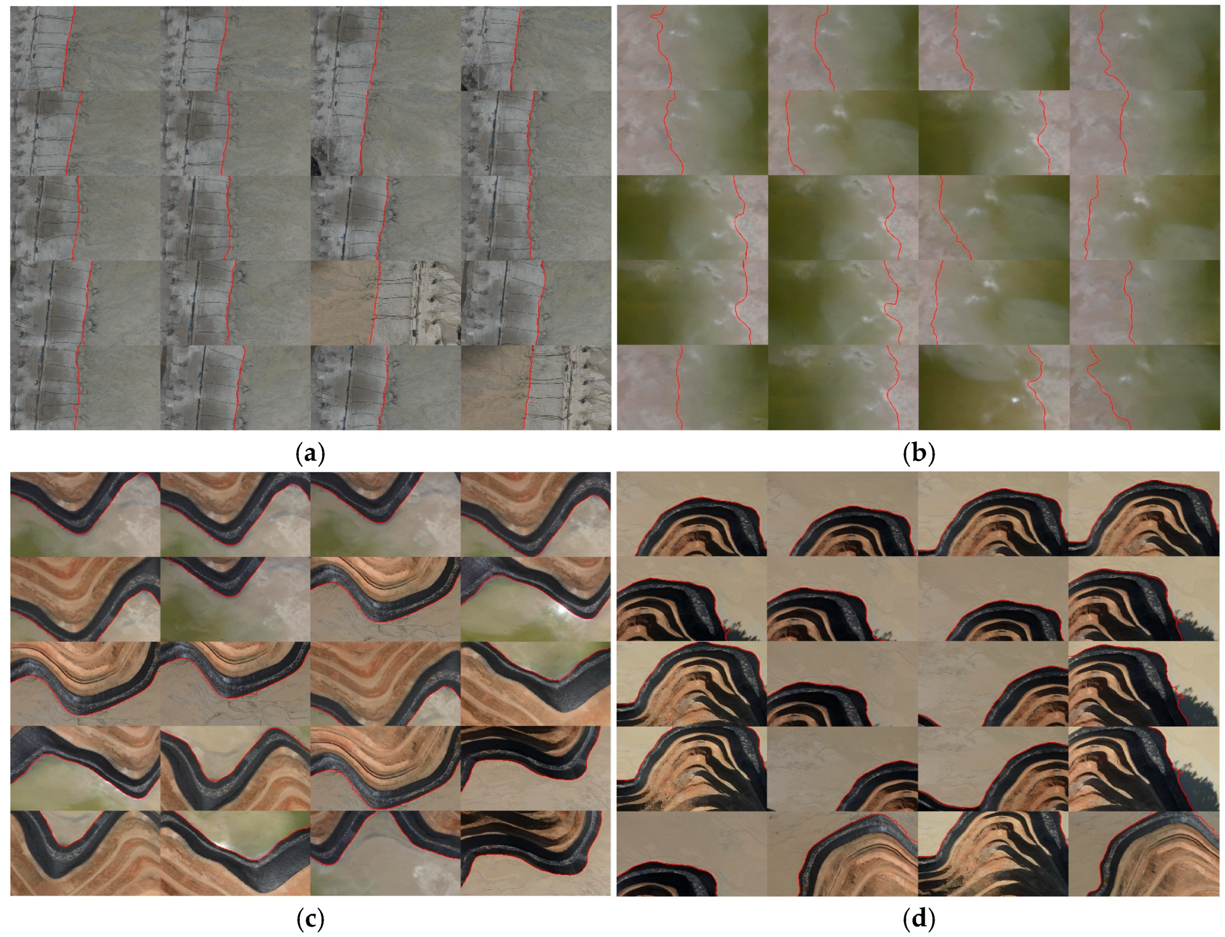
To accurately map dry beach boundaries from 2D semantic masks to 3D space, a boundary pixel extraction and back-projection method is employed in this study. First, the Canny edge detection algorithm is applied to the semantic segmentation results to identify 2D boundary pixels between “dry beach” and “non-dry beach” regions, as illustrated in Figure 8. Each boundary pixel is then back-projected into 3D space using the known projection matrix obtained from the 3D reconstruction, forming a ray along which the nearest point in the reconstructed dense point cloud is determined as its 3D coordinate (Equation (6)). Once all boundary pixels are processed, the resulting 3D boundary points are projected onto the XOY plane and fitted with a closed polygon. Points inside the polygon are classified as dry beach, while those outsides are considered non-target features (e.g., dams, hillslopes, water). This approach successfully integrates 2D semantic information with 3D geometric constraints, enabling efficient extraction of dry beach from large-scale point clouds.

3. Experiments and Results

3.1. Data Acquisition

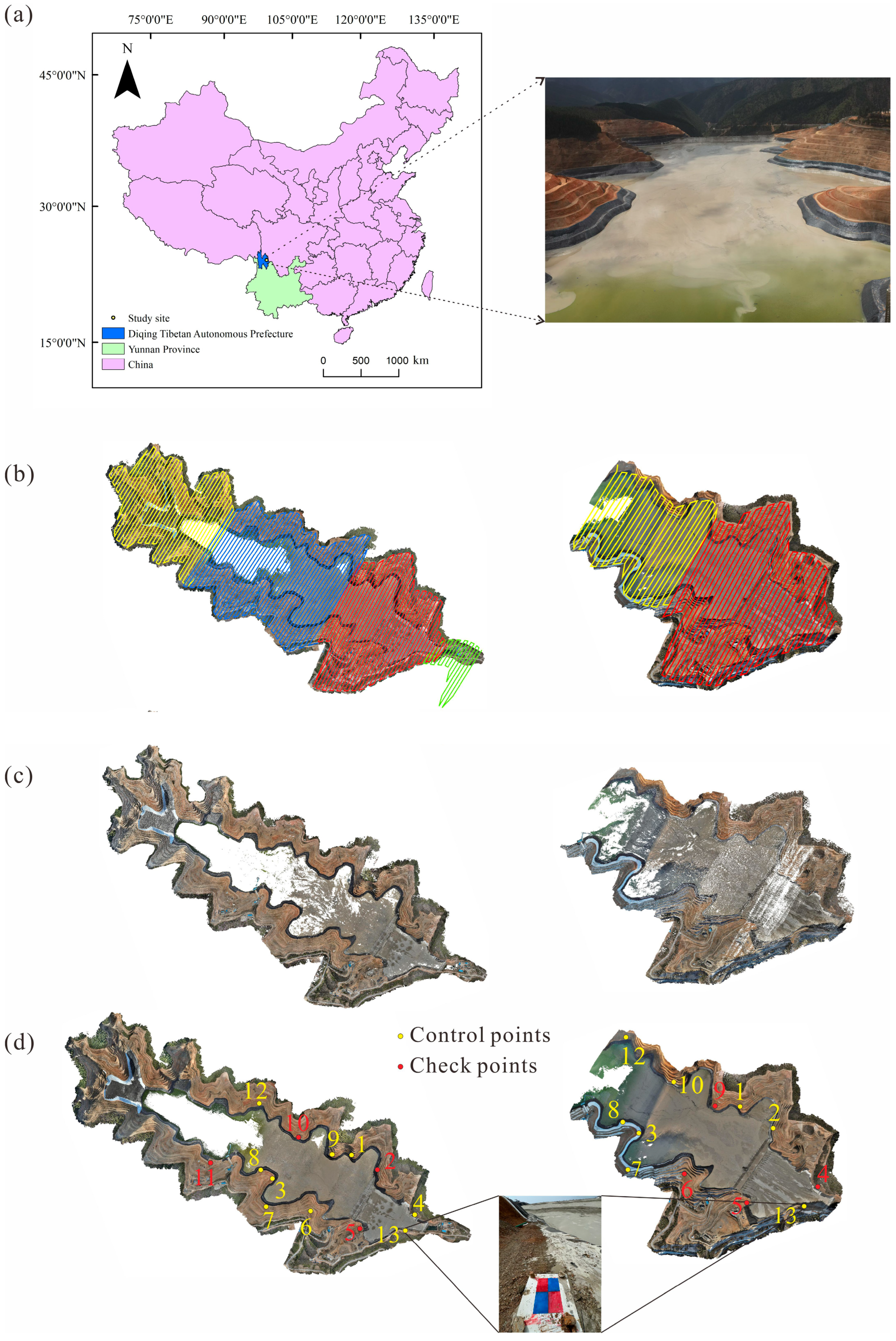
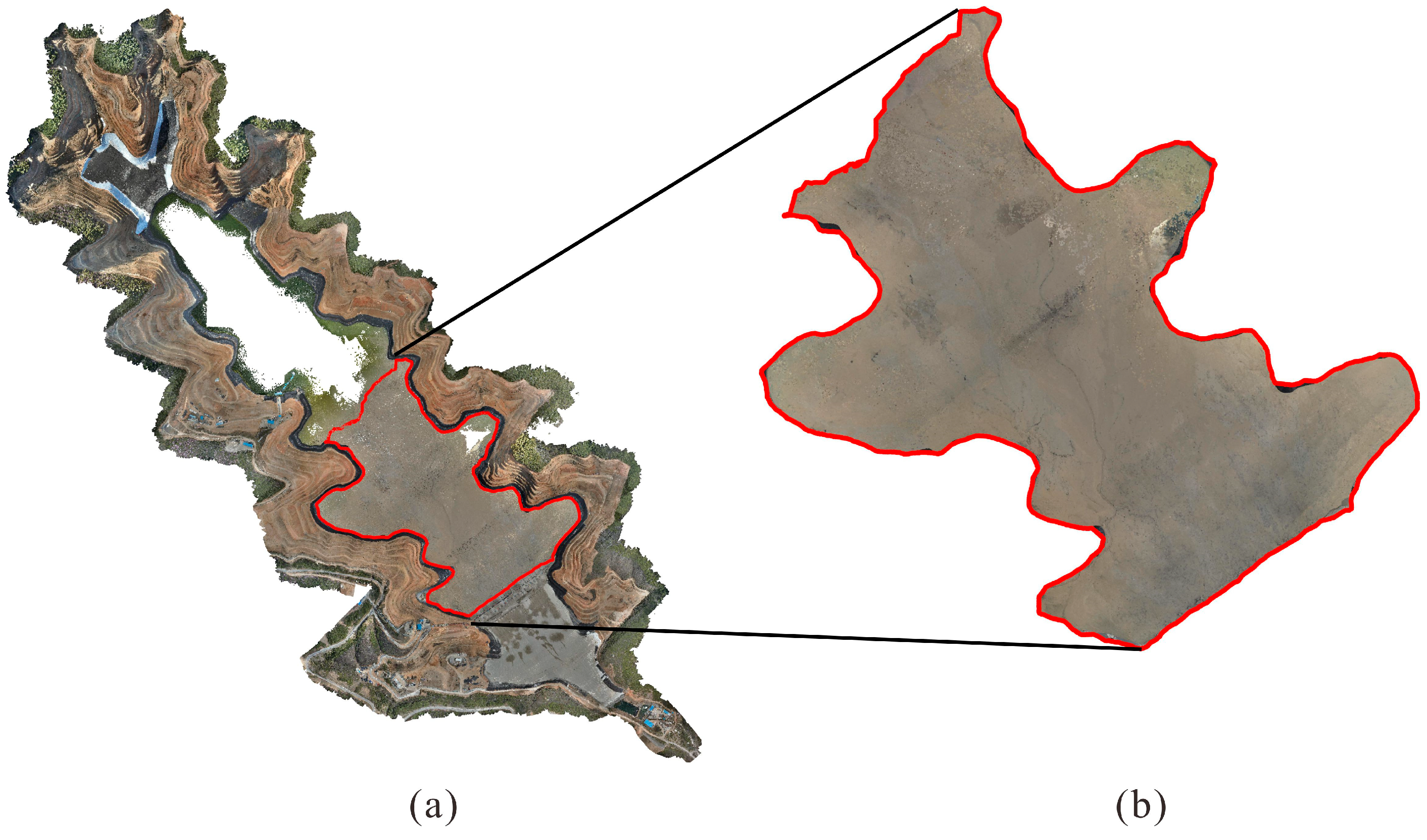
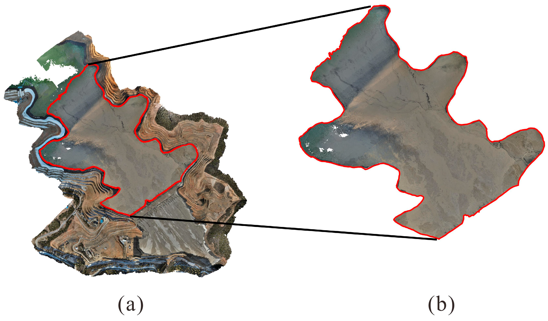
The study area is a valley-type tailings pond located in Yunnan Province, China, with an altitude of approximately 3300–3560 m (Figure 9a). The pond extends roughly 4–6 km along a northwest–southeast trending valley, with a floor width of about 100 m and side slopes of 25–35°, representing a typical morphology of mountainous tailings ponds. The narrow, elongated valley-type morphology of the pond reflects the typical spatial arrangement of dry beaches. The lithology is dominated by weakly metamorphosed slate, with well-developed shear joints and cleavage. Surface water is primarily supplied by the Gecan River system and groundwater is primarily fissure water within the slate, supplemented by scattered pore water in loose deposits. The region experiences pronounced seasonal precipitation, with nearly 90% of annual rainfall occurring during the wet season from May to September, while winter months are cold and mining activities are typically limited.

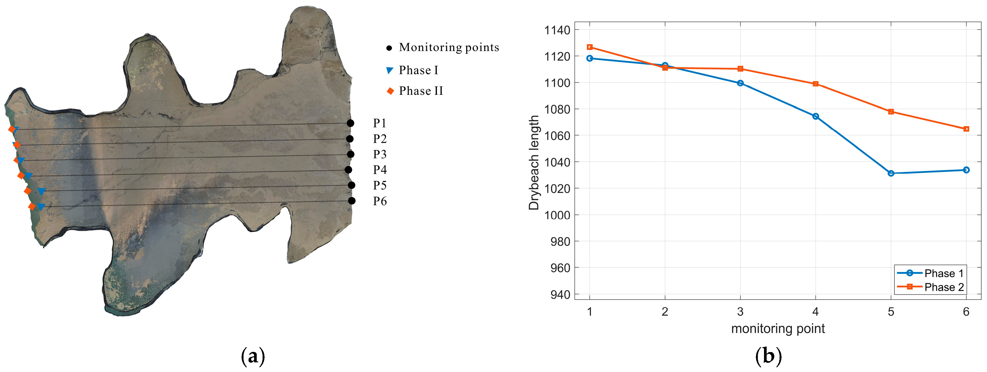
To validate the applicability and generalization capability of the proposed method, UAV data were collected in two phases: May 2024 (phase I) and January 2025 (phase II). Phase I was acquired during the wet season, when precipitation is concentrated, and the reservoir water level is relatively high, resulting in partial inundation of the dry beach and a relatively shorter exposed beach length. In contrast, phase II was conducted during the cold and dry winter period at a high altitude. During this period, mining activities were suspended, tailings discharge was significantly reduced, and parts of the reservoir surface were frozen, leading to changes in surface reflectance and enhanced brightness contrast between the water and dry beach boundaries. Meanwhile, snow cover occurred on portions of the hillslopes, and strong surface reflections were introduced due to low solar elevation. In addition, the seasonal replacement of black tarpaulins with white ones altered the surface appearance. Therefore, the two phases represent contrasting acquisition conditions in terms of hydrology, surface cover, and illumination, providing a suitable multi-temporal dataset for evaluating the robustness of boundary extraction. Both datasets cover the tailings dam, dry beach, reservoir water, and surrounding hills, providing typical samples with clear boundary structures and diverse terrain.

For high-precision modeling and boundary identification of the tailings pond, multi-view images were acquired using a DJI M300 RTK drone with a Zenmuse P1 camera. As phase I was the initial survey, the flight route was designed to ensure full coverage of the entire study area, with a flight altitude of approximately 145 m and a coverage area of about 3.85 km². In phase II, the flight route was optimized to improve acquisition efficiency while still ensuring complete coverage of the target area, resulting in a reduced flight altitude of approximately 127 m and a smaller coverage area of about 1.23 km². Therefore, four sub-area flights were conducted in phase I and two in phase II, each with at least 80% forward overlap and 70% side overlap to ensure reliable 3D reconstruction (Figure 9b). Thirteen targets were deployed throughout the study area (Figure 9d), and their coordinates were precisely measured using RTK. In phase I, nine of them were used as Ground Control Points (GCPs) to constrain the bundle adjustment, while the remaining four were reserved as independent Check Points (CKPs) for accuracy assessment. In phase II, due to the optimized flight route, one target (Point 11) was not captured, resulting in twelve valid targets, among which eight were used as GCPs and four as CKPs to maintain a consistent validation.

A total of 4016 and 3985 original images were acquired for phase I and phase II, respectively, with each image having a resolution of 8192 × 5460 pixels. SfM and MVS techniques were applied to generate approximately 3.97 million sparse points and 240.8 million dense points in phase I, and 1.71 million sparse points and 177.5 million dense points in phase II, as shown in Figure 9c,d. The accuracy assessment is summarized in

Table 1. Accuracy evaluation of GCPs and CKPs for phase I and phase II.

Phase I						Phase II
GCPs			CKPs			GCPs			CKPs
No.	Error (cm)		No.	Error (cm)		No.	Error (cm)		No.	Error (cm)
	XY	Z		XY	Z		XY	Z		XY	Z
1	5.93	0.68	2	1.83	6.04	1	1.80	3.39	4	2.92	2.94
3	4.85	0.48	5	4.02	1.13	2	2.06	0.70	5	1.06	2.76
4	9.68	6.97	10	3.61	4.44	3	3.39	1.66	6	1.05	3.72
6	4.51	1.09	11	2.18	4.83	7	1.42	2.12	9	2.68	4.01
7	1.20	0.12	-	-	-	8	2.02	0.12	-	-	-
8	0.76	0.91	-	-	-	10	0.16	1.42	-	-	-
9	3.15	0.01	-	-	-	12	1.95	2.41	-	-	-
12	1.95	0.18	-	-	-	13	3.53	0.73	-	-	-
13	0.81	0.73	-	-	-	-	-	-	-	-	-
RMSE	4.58	2.40		3.05	4.49		2.28	1.86		2.12	3.40

. The root mean square error (RMSE) of CKPs for phase I was ± 3.05 cm (horizontal xy) and ± 4.49 cm (vertical z), while phase II was ± 2.12 cm (horizontal xy) and ± 3.40 cm (vertical z). The errors of the CKPs were consistent in magnitude with the residuals of the GCPs, demonstrating the high reliability of the photogrammetric reconstructions. This level of accuracy is sufficient to meet the engineering requirements of the present study.

Both datasets effectively reconstructed the 3D structure of the tailings dam, dry beach, and reservoir water area. Projection matrices for all images were also obtained during the reconstruction process, enabling subsequent 3D back-projection of semantic boundaries.

3.2. Network Comparison

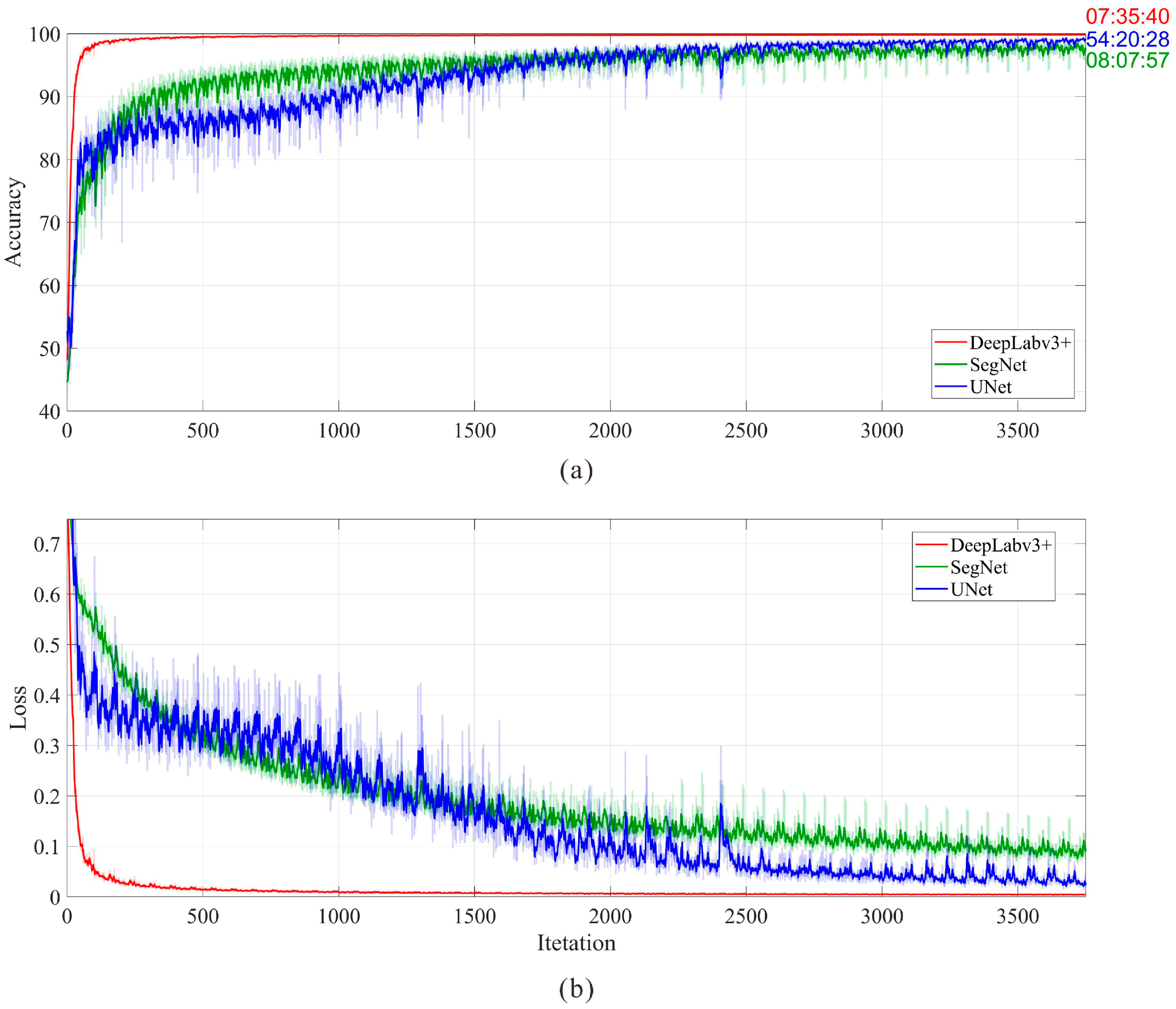
To evaluate the suitability of the different semantic segmentation networks for dry beach identification, three classical networks (DeepLabv3+, SegNet [59], and UNet [60]) were compared using identical datasets, augmentation strategies, and training parameters. Figure 10 illustrates the training processes of the three networks. With the same number of iterations, DeepLabv3+ (7.5 h) and SegNet (8 h) required far less training time than UNet (54.5 h). More importantly, the learning curve indicates that DeepLabv3+ reached near-convergence significantly earlier than both SegNet and UNet, while consistently maintaining higher accuracy. These results demonstrate the clear advantages of DeepLabv3+ in both training efficiency and performance.

To quantitatively evaluate model performance, three commonly used evaluation metrics are adopted. Accuracy is the ratio of correctly predicted pixels to the total ground truth pixels for a given class. Intersection over Union (IoU) is the ratio of correctly classified pixels to the total number of ground truth and predicted pixels in that class. Boundary F1 Score (BF) quantifies boundary extraction accuracy by comparing predicted boundaries with ground truth, with higher scores indicating better matching.

Table 2. The mean value of the evaluation metrics based on the test data.

	Mean Accuracy	Mean IoU	Mean BF
DeepLabv3+	0.9642	0.9349	0.8072
SegNet	0.9230	0.8782	0.5133
UNet	0.8665	0.7723	0.5791

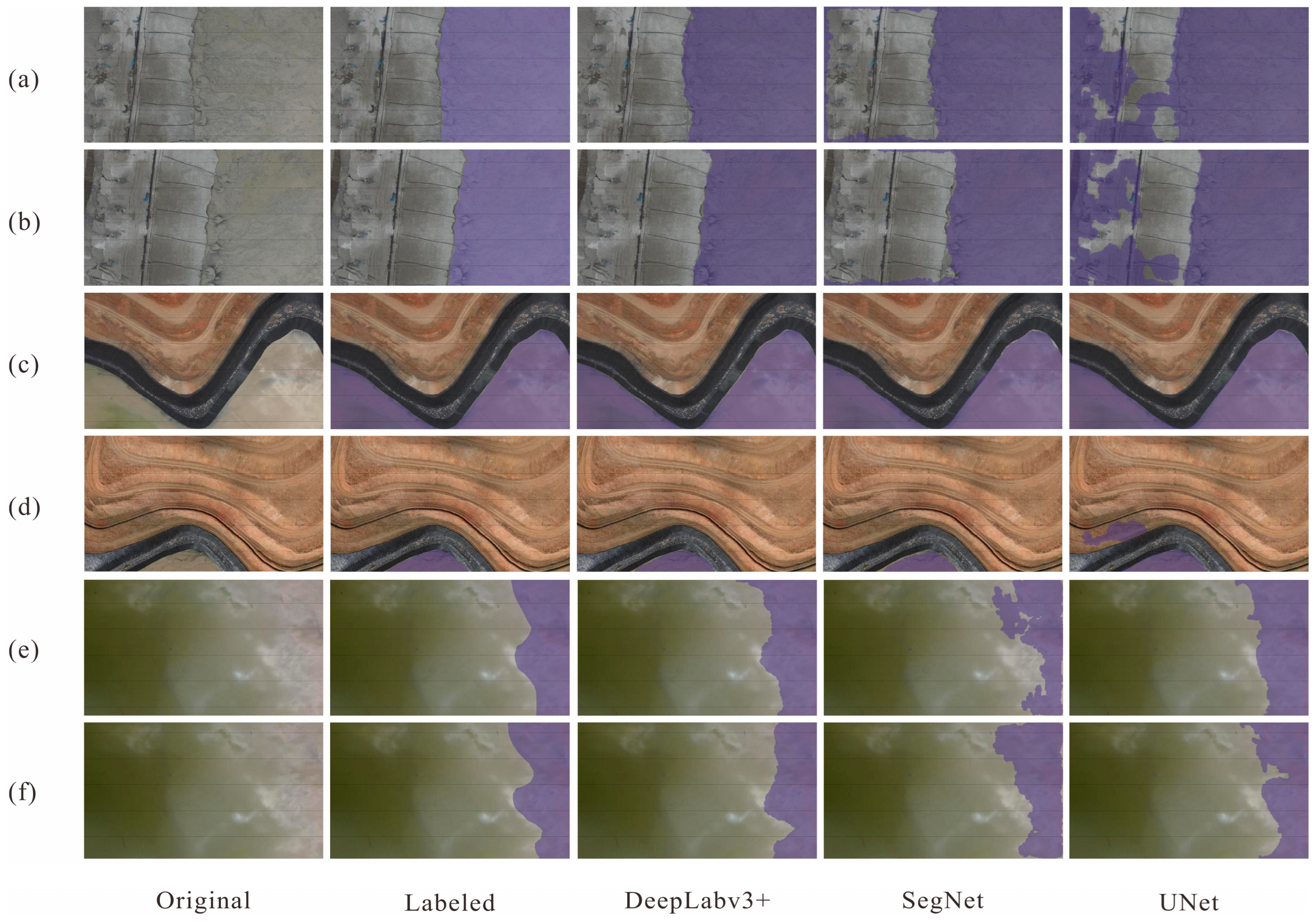
summarizes the mean values of three evaluation metrics across all classes on the test set for the three networks. Figure 11 shows representative segmentation results compared with the ground truth. DeepLabv3+ achieves the highest scores across all indices, producing precise boundaries and structural continuity. SegNet exhibits moderate accuracy but poor boundary delineation (BF = 0.5133). This is visually manifested as blurred and discontinuous boundaries deviating from the true edges (Figure 11). UNet shows relatively lower overall accuracy, although its mean BF (0.5791) is slightly higher than that of SegNet. However, UNet generated noticeable misclassifications in several cases. Overall, DeepLabv3+ demonstrates optimal performance in both training efficiency and segmentation quality, establishing it as the preferred network for dry beach boundary identification in this study.

3.3. Results of Phase I

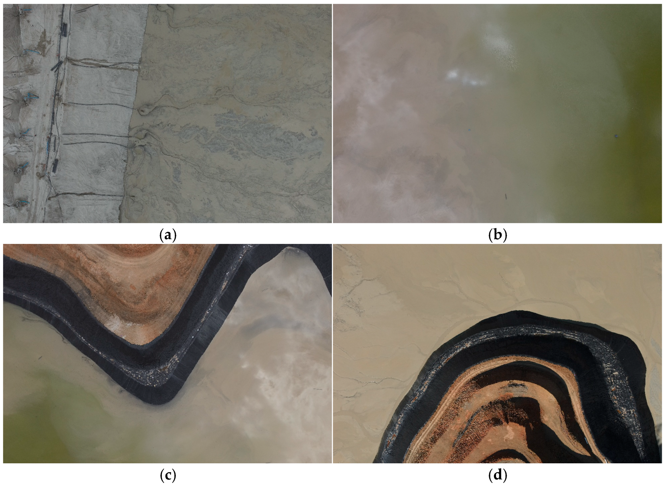
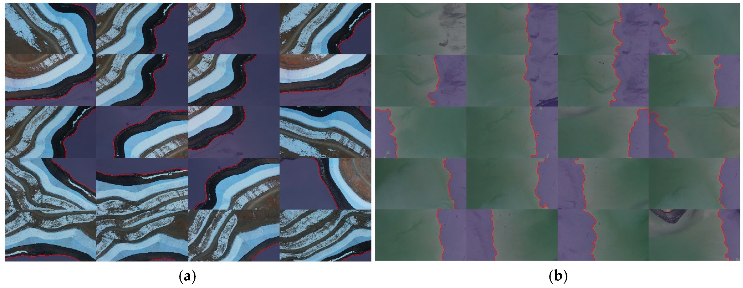
Four representative boundary images in Figure 12 were selected as templates. The similarity between all images and templates was calculated using Equations (7)–(9). The weighting coefficient r = 0.5 was set to assign equal importance to the features extracted by AlexNet and GoogLeNet. With a threshold of K = 0.35, the retrieval process identified 152 dry beach-dam boundary images from the template in Figure 12a, 248 waterline images from Figure 12b, and 211 and 214 dry beach-hillside boundary images from Figure 12c and Figure 12d, respectively. Examples of the retrieved images are shown in Figure 13.

The retrieved images were then segmented into “dry beach” and “non-dry beach” regions using the trained DeepLabv3+ model (Section 2.3.2). Figure 14 shows segmentation examples corresponding to the images in Figure 13. To quantitatively evaluate the segmentation performance of the proposed method in phase I images, the images shown in Figure 13 were manually annotated and compared with the automatic segmentation results.

Table 3. The mean evaluation metrics for the representative phase I images are shown in Figure 13.

	Mean Accuracy	Mean IoU	Mean BF
dry beach—dam	0.9931	0.9862	0.8890
dry beach—reservoir water	0.9101	0.8477	0.7059
dry beach—hillside 1	0.9871	0.9713	0.8611
dry beach—hillside 2	0.9805	0.9614	0.8507
Mean	0.9677	0.9417	0.8267

lists the three evaluation metrics, including accuracy, Intersection over Union (IoU), and Boundary F1 Score (BF).

For the dam boundary and hillside boundary, both the mean accuracy and IoU consistently exceeded 0.95, indicating that the segmented dry beach regions exhibit high regional completeness without obvious misclassification. In addition, the mean BF for these boundaries reached values above 0.85, demonstrating a high consistency between the extracted boundaries and the manually interpreted ones. A comparison between the dry beach-hillside 1 and hillside 2 shows that the performance of hillside 2 is slightly lower. This discrepancy is mainly attributed to shadow effects induced by vegetation projected onto the dry beach under oblique illumination conditions. The shadowed areas exhibit spectral characteristics similar to black tarpaulins on the hillside, resulting in partial misclassification of dry beach pixels as background (Figure 14d).

For the water boundary, the evaluation metrics are relatively lower, with mean accuracy, IoU, and BF of approximately 0.9101, 0.8477, and 0.7059, respectively. This is mainly because the transition zone between water and dry beach is inherently ambiguous, where water and deposited materials are intermingled. Consequently, both manual annotation and automatic segmentation suffer from unavoidable uncertainties near the transition zone.

Canny edge detection was subsequently applied to the extracted 2D boundary pixels from the segmented images, with results illustrated in Figure 15. Next, the 2D boundary pixels were back-projected to 3D space using the projection matrices obtained from SfM reconstruction. For each pixel, a ray was constructed along the back-projection direction, and the nearest neighbor in the dense point cloud was selected as the 3D coordinate, producing a set of 3D boundary points (Figure 16a). These 3D boundary points were projected onto the XOY plane and fitted with a closed 2D polygon. The dense point cloud was then clipped through a spatial inclusion test to isolate the dry beach points (Figure 16b). The resulting point cloud exhibits clear coverage and structural continuity, providing a reliable basis for further geometric analyses.

3.4. Results of Phase II

To assess the temporal adaptability of the proposed method, the semantic segmentation model trained on phase I was directly applied to the phase II dataset. Differences in imaging conditions and environmental states between the two phases affected the stability and generalization performance of the model. From the 3985 images in phase II, 653 boundary images were identified, including 62 dry beach-dam boundaries, 343 dry beach-hillslope boundaries, and 152 waterline boundaries. Typical examples are shown in Figure 17, with the first image serving as the template.

The segmentation performance in phase II images was evaluated using manually annotated boundaries in the same manner as in phase I (

Table 4. The mean evaluation metrics for the representative phase II images are shown in Figure 17.

	Mean Accuracy	Mean IoU	Mean BF
dry beach—dam	0.9874	0.9797	0.8802
dry beach—reservoir water	0. 8501	0.7841	0.6114
dry beach—hillside	0.9314	0.9186	0.8043
Mean	0.9230	0.8941	0.7653

). The results indicate that the model maintained good performance in certain regions of phase II. For the dam boundary, the evaluation metrics remain comparable to those in phase I, due to the clear structural outlines (Figure 17a), indicating that the proposed model maintains stable performance.

The hillside boundary (Figure 17c) was also segmented accurately under varying illumination and shadows, reflecting a reasonable generalization. However, the evaluation metrics show a decrease, with mean accuracy, IoU, and BF dropping to approximately 0.9314, 0.9186, and 0.8043, respectively. This degradation is mainly caused by surface changes between the two periods. Some hillside boundary images of phase II included white coverings such as snow and white tarpaulins, whereas phase I images featured black tarpaulins partially obscuring the hillside. These variations in color and texture degrade the model generalization, leading to misclassifications in the affected regions (Figure 17c).

For the water boundary in phase II, the performance also exhibits a certain degree of degradation (Figure 17b). In phase I, the uncertainty mainly originates from the inherent mixing characteristics of the transition zone, which makes the boundary ambiguous. In phase II, however, the performance degradation is additionally closely related to the changes in illumination conditions. Compared with the dam and hillslope regions, the water surface is more sensitive to illumination variations, and changes in optical reflection properties cause the visual features of part of the dry beach-reservoir water transition zone to deviate from the feature distribution learned from the phase I training data. As a result, when the model trained only in phase I images is directly applied to the phase II dataset, a decrease in segmentation robustness is observed in the water boundary regions.

4. Discussion

4.1. Analysis of Generalization Capability

As discussed in Section 3.4, although some regions in phase II exhibited boundary blurring and misclassifications, the overall structural continuity of the boundaries was preserved. However, these errors revealed model generalization limitations when faced with variations in surface cover and reflections. To enhance robustness under such challenging conditions, a lightweight incremental training strategy was implemented. The model was fine-tuned using only 8 annotated phase II images (2 hillside boundaries and 6 waterline boundaries) (Figure 18), which were augmented to 200 training samples.

The results demonstrate a clear improvement in segmentation accuracy for hillside regions and more distinct boundaries in waterline regions, as shown in Figure 19. Figure 20 shows the corresponding 3D boundary and dry beach point cloud after fine-tuning. Overall, the experiments demonstrate the cross-phase generalization capability of the proposed method. The lightweight incremental training approach reduces deployment costs and demonstrates practical potential. Moreover, integrating continual learning techniques in future work could further improve adaptability to extreme conditions.

4.2. Traditional Point Cloud Segmentation

Two conventional point cloud segmentation techniques were also evaluated: Region Growing (RG) and Random Sample Consensus (RANSAC). RG clusters point clouds based on geometric similarity using normal vector and curvature as growth criteria. However, inconsistent normal and significant curvature variations caused by sediment accumulation and local subsidence in the dry beach compromise the segmentation consistency. As shown in Figure 21a, RG incorrectly merges the dry beach with the tailings dam into a continuous structure and produces fragmented segments near the waterside. RANSAC, which fits geometric primitives (e.g., planes, cylinders) through random sampling and consensus evaluation, is similarly challenged by the complex micro-topography and elevation variations in the dry beach. As shown in Figure 21b, it overextends boundaries and captures water–hillside interfaces as well as portions of the water surface.

In summary, the performance of RG and RANSAC is constrained by their dependence on geometric assumptions, rendering them inadequate for precise dry beach boundary extraction. In contrast, our method exploits deep networks to extract high-level semantic features from images and reconstructs accurate 3D boundaries through projection matrices.

4.3. Dry Beach Monitoring

The proposed method not only enables automated extraction of 3D dry beach boundaries but also quantitative monitoring of safety indicators and deposition changes. First, dry beach length can be derived from reconstructed 3D boundaries. Monitoring across five sections (Figure 22a) indicates an average variation of 20.4 m. Given that the minimum dry beach length influences the phreatic line position, particular concern is paid to point P5, where a 64.1 m reduction was observed between the two phases (Figure 22b). Such variations reflect seasonal hydrological conditions: higher water levels during May rainfall shorten the dry beach, whereas lower levels in drier January expose more of it. Second, the results support multi-temporal deposition analysis through point cloud registration and vertical differences analysis. A sectional profile of the dry beach point cloud is shown in Figure 23a, where noise points are distributed along the Z-direction on both sides of the dry beach surface, while points on the actual surface exhibit the highest density, and the surrounding sparse points are considered noise. Considering this characteristic, the dry beach point clouds were denoised using a density-based filtering method on sectional profiles, in which points with the maximum Z-direction density were retained as valid points (Figure 23a). Then, pairwise comparisons of the denoised multi-temporal dry beach point clouds were conducted. As shown in Figure 23b, deposition is concentrated along the main discharge channel, while regions near the reservoir water show minimal elevation change. These results demonstrate the spatial heterogeneity of tailings discharge and deposition thickness, providing a crucial 3D dataset for characterizing depositional processes.

5. Conclusions

In this study, we proposed a deep learning–based framework that integrates image semantic segmentation with 3D reconstruction to accurately extract dry beach boundaries from UAV datasets, establishing a complete workflow from boundary image retrieval and semantic segmentation to 3D back-projection and dry beach point cloud extraction.

The proposed method was first applied to phase I images, where DeepLabv3+, SegNet, and Unet were trained on a limited number of annotated images. Comparative experiments indicate that DeepLabv3+ achieved higher segmentation accuracy, Intersection over Union (IoU), and Boundary F1 score (BF), making it a suitable choice for this study. The results of phase I demonstrate that the proposed framework can effectively extract continuous boundaries and point clouds of the dry beach.

When the model trained in phase I images is directly applied to the phase II dataset, the performance remains generally stable for dam and partial hillslope boundaries, while certain degradations occur in regions affected by surface cover changes and illumination variations. These issues can be effectively mitigated through fine-tuning with a small number of additional samples, confirming the feasibility of the lightweight incremental training strategy.

Unlike traditional point-cloud segmentation that relies on geometric conditions, the proposed approach effectively handles irregular boundaries and complex textures. The extracted 3D boundaries and dry beach point cloud enable the quantitative analysis of length and morphology changes, overcoming the limitations of purely 2D image analyses.

In this work, AlexNet and GoogLeNet were employed for image feature extraction, and DeepLabv3+ was used for semantic segmentation. Although these are classical network architectures, the experimental results demonstrate that the extracted boundary images and segmentation outputs are sufficient for practical engineering applications. Future work will explore the integration of more recent network architectures and more challenging image scenarios to further improve the robustness and efficiency of the proposed framework. Overall, the proposed framework provides a reliable and scalable solution for automated 3D monitoring of tailings beaches, supporting safety assessment and multi-temporal deposition analysis in engineering applications.