PMSAF-Net: A Progressive Multi-Scale Asymmetric Fusion Network for Lightweight and Multi-Platform Thin Cloud Removal

Highlights

What are the main findings?

• Lightweight Network Design: PMSAF-Net, a lightweight Progressive Multi-Scale Asymmetric Fusion Network, is proposed for efficient thin cloud removal in remote sensing images. It achieves favorable performance with only 0.32 M parameters, making it suitable for multi-platform deployment.
• A multi-scale fusion architecture with an asymmetric attention mechanism: The proposed framework effectively captures detailed cloud information while reducing computational costs by incorporating a Dual-Branch Asymmetric Attention mechanism (DBAA) with parallel pathways for efficient feature enhancement and a hierarchical multi-scale fusion module Multi-Scale Context Aggregation (MSCA) featuring a coarse-to-fine processing pipeline.

What is the implication of the main finding?

• It provides a practical lightweight architecture for multi-platform deployment. The model’s extreme efficiency and performance demonstrate a viable path for deploying advanced deep learning-based restoration tasks like cloud removal directly on resource-constrained edge devices such as satellites and drones, which is a core goal of multi-platform remote sensing.

Abstract

With the rapid improvement of deep learning, significant progress has been made in cloud removal for remote sensing images (RSIs). However, the practical deployment of existing methods on multi-platform devices faces several limitations, including high computational complexity preventing real-time processing, substantial hardware resource demands that are unsuitable for edge devices, and inadequate performance in complex cloud scenarios. To address these challenges, we propose PMSAF-Net, a lightweight Progressive Multi-Scale Asymmetric Fusion Network designed for efficient thin cloud removal. The proposed network employs a Dual-Branch Asymmetric Attention (DBAA) module to optimize spatial details and channel dependencies, reducing computation cost while improving feature extraction. A Multi-Scale Context Aggregation (MSCA) mechanism captures multi-level contextual information through hierarchical dilated convolutions, effectively handling clouds of varying scales and complexities. A Refined Residual Block (RRB) minimizes boundary artifacts through reflection padding and residual calibration. Additionally, an Iterative Feature Refinement (IFR) module progressively enhances feature representations via dense cross-stage connections. Extensive experimental multi-platform datasets results show that the proposed method achieves favorable performance against state-of-the-art algorithms. With only 0.32 M parameters, PMSAF-Net maintains low computational costs, demonstrating its strong potential for multi-platform deployment on resource-constrained edge devices.

1. Introduction

Remote Sensing Images (RSIs) play an important role in global environmental science [1], resource management [2], urban planning [3], disaster monitoring [4] and military surveillance [5]. A major challenge is cloud cover, which has a global annual average of over 66% [6]. Thin cloud removal is essential to maximize the utility of RSIs. However, current methods face three fundamental limitations that hinder their practical deployment on multi-platform devices:

1.

Real-time Processing Constraints: Most deep learning-based approaches involve high computational complexity, with block-based algorithms requiring up to ${10}^8$ operations for standard 512 × 512 images [7]. This prevents millisecond-level response times required for drone-based monitoring and other real-time applications.

2.

Hardware Resource Limitations: Transformer-based and hybrid approaches demand substantial GPU memory and multi-GPU setups [8,9], making them unsuitable for deployment on resource-constrained edge devices in multi-platform scenarios (e.g., onboard satellites, aircraft systems with strict power budgets).

3.

Performance Gaps in Multi-Scale Complex Scenarios: Physics-based methods fail with complex cloud distributions [10], while single-scale CNN architectures struggle with the nature of multi-platform data, leading to incomplete removal and detail loss [11].

To tackle these issues, we propose PMSAF-Net, a lightweight network designed for thin cloud removal with multi-platform deployment in mind. Our approach addresses these limitations by integrating adapted modules: DBAA adapts parallel attention, MSCA builds on dilated convolutions, RRB modifies residual blocks, and all work together for lightweight cloud removal. Experiments demonstrate that our model achieves competitive performance with only 0.32 M parameters, making it a suitable and efficient solution for multi-platform remote sensing scenarios.

Thin clouds, as one of the most prevalent atmospheric phenomena, are characterized by low optical thickness and high transparency. When input images are degraded by thin clouds, the performance of subsequent image processing algorithms is inevitably compromised. Through spectral modeling and convolutional neural networks (CNNs), thin cloud removal algorithms aim to eliminate cloud interference and retrieve the true surface reflectance. For thin cloud removal, the degradation model of cloud removal can be commonly described as follows [12]:

$$I\left(x\right)=J\left(x\right)·t\left(x\right)+A·(1-t(x\left)\right)$$

(1)

where x is the position of the pixel, $J\left(x\right)$ denotes a haze-free image, and $I\left(x\right)$ represents an observed cloudy image, respectively, A is the global atmospheric light, and t represents the medium transmission map. Solving Equation (1) is challenging because the number of unknowns exceeds the knowns, making cloud removal an ill-posed problem. While numerous cloud removal methods achieve satisfactory restoration accuracy, their computational complexity typically precludes real-time implementation in latency-sensitive applications. These limitations necessitate the development of lightweight algorithms, which have attracted growing attention due to their computational efficiency and real-time processing capabilities. The primary contribution of this work is the effective integration and adaptation of established deep learning components into a cohesive and efficient architecture for thin cloud removal, which is summarized as follows:

1.

A Co-Designed Lightweight Framework for Practical Cloud Removal. We present PMSAF-Net, a network that innovates through the synergistic integration of adapted, existing techniques (e.g., attention, dilated convolutions). This co-design achieves an optimal balance between accuracy and efficiency, attaining 27.258 dB PSNR on RICE1 with only 0.32 M parameters, making it suitable for deployment on drones and satellites.

2.

Efficiency-Oriented Component Adaptations. The framework is realized through two tailored modules. A Dual-Branch Asymmetric Attention mechanism that reduces computational redundancy, cutting parameters by 6% while improving PSNR by 0.863 dB. A Multi-Scale Context Aggregation module that captures varying cloud patterns without parameter increase, yielding a 0.361 dB PSNR gain with 6% fewer parameters.

3.

A Demonstrated Paradigm for Engineering Value. The core contribution lies in demonstrating that strategic integration and adaptation can turn established techniques into an effective, lightweight solution for a specific real-world problem. This work provides a practical blueprint for high-performance cloud removal under stringent resource constraints.

2. Related Work

The past decade has seen remarkable advancements in remote sensing technologies, leading to significant progress in cloud removal methods. These include physics-based approaches, traditional digital image processing, statistical learning methods, deep learning architectures, and hybrid approaches. Cloud removal methods have evolved from physics-based and traditional models to deep learning approaches. While effective, these methods often face a trade-off between performance and computational cost, making them unsuitable for resource-constrained multi-platform deployment [7,8,9]. Physics-based methods and traditional digital image processing are suitable for simple scenarios due to low resource consumption [10,13]. statistical learning, with moderate resource needs, lacks generalization and relies on manual engineering [14].

Practical applications in aerospace and aviation impose critical hardware resource constraints. In such contexts, CNN-based architectures are recognized for achieving an optimal balance between performance and resource consumption [15]. While deep learning excels through automatic feature learning, this capability comes at a cost. The practical deployment of many powerful models, including Transformers and very deep CNNs, is often hampered by their large parameter footprint. To directly address this limitation of parameter inefficiency, our work proposes a lightweight network that requires far fewer parameters. Furthermore, CNN-based design avoids the memory explosion typical of Transformers [8] and outperforms physics-based methods in handling heterogeneous cloud cover [16]. Although hybrid approaches can achieve top performance, their excessive complexity and resource demands [17] often preclude their use in resource- constrained systems.

Recent advances in lightweight networks prioritize computational efficiency for on-device deployment. Architectures like MobileNet [18] use depthwise separable convolutions to reduce parameters. ShuffleNet [19] employs channel shuffle to maintain information flow. In remote sensing, dedicated designs such as CloudSatNet-1 [15] prove the viability of quantized CNNs for satellite processing. Our work builds directly upon Half-UNet [20]. We selected it for its streamlined encoder-decoder structure. This architecture provides an ideal balance between structural simplicity and representation capability. It offers a clean and efficient foundation for integrating our proposed asymmetric attention and multi-scale fusion modules.

3. Methods

This section details the proposed PMSAF-Net. To address the computational overhead and hardware constraints in multi-platform remote sensing image processing, we propose a network that integrates four key innovations to achieve an accuracy-efficiency trade-off. The motivation is introduced in Section 3.1. The overall architecture is introduced in Section 3.2. The network integrates four key components: a DBAA module for efficient feature refinement in Section 3.3, an MSCA module for handling varying cloud scales in Section 3.4, an RRB for artifact reduction in Section 3.5, and an IFR module for progressive enhancement in Section 3.6.

3.1. Motivation

The growing demand for lightweight networks has motivated architectures like Half-UNet [20], which simplifies U-Net by removing its decoder and skip connections to reduce complexity. However, it faces three key limitations: its single-scale processing fails to adapt to varying object sizes, causing information loss [21]; its lack of feature prioritization wastes computational resources [21]; and its standard convolutions propagate feature errors, lowering reconstruction accuracy [20]. To overcome these issues under hardware constraints, our work introduces targeted solutions for attention enhancement, multi-scale context, residual optimization, and hierarchical refinement.

3.2. Overall Network Architecture

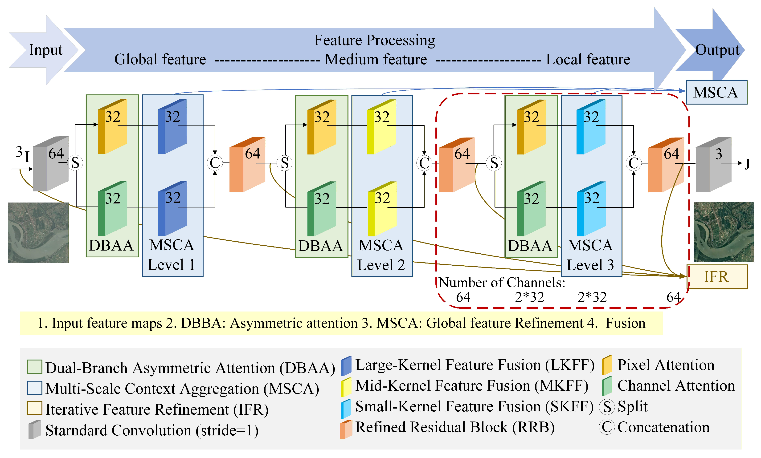
The overall architecture of the proposed PMSAF-Net, designed for thin cloud removal across multi-platform remote sensing data, is illustrated in Figure 1. The diagram employs a color-coding scheme to distinguish different operational modules: for instance, green blocks represent the DBAA module, while blue blocks correspond to the MSCA modules, with the specific level (e.g., Level 1) indicated within each block. The network implements a parallel multi-scale fusion architecture with dual attention mechanisms to efficiently process features. It processes input features through three serial pathways. Each pathway first applies the DBAA module for efficient feature refinement, then leverages size-specific MSCA modules to capture cloud patterns at various scales, and finally achieves reconstruction via hierarchical feature fusion.

The overall processing flow of PMSAF-Net is formally described below. It consists of three specialized streams through which input features progress for multi-scale extraction. The serial processing flow is defined as follows:

$$\begin{array}{cc}\hfill & \mathrm{Let}\hfill \\ \hfill & S_1^{\mathrm{out}}={\mathrm{Stream}}_1({\mathcal{F}}_{\mathrm{in}};{\mathcal{K}}_{11\times 11},{\mathcal{K}}_{7\times 7})\hfill \\ \hfill & S_2^{\mathrm{out}}={\mathrm{Stream}}_2(S_1^{\mathrm{out}};{\mathcal{K}}_{3\times 3})\hfill \\ \hfill & S_3^{\mathrm{out}}={\mathrm{Stream}}_3\left(S_2^{\mathrm{out}}\right)\hfill \\ \hfill & {\mathcal{F}}_{\mathrm{fused}}=\mathrm{IFR}(S_1^{\mathrm{out}},S_2^{\mathrm{out}},S_3^{\mathrm{out}})\hfill \\ \hfill & {\mathcal{F}}_{\mathrm{out}}={\Phi }_{\mathrm{conv}}\left({\mathcal{F}}_{\mathrm{fused}}\right)\hfill \end{array}$$

(2)

where ${\mathcal{F}}_{out}$ represents the final output image with 3 RGB channels, ${\Phi }_{conv}$ represents the output convolution, $IFR$ represents the IFR module for cross-stream fusion, ${Stream}_1,{Stream}_2$, ${Stream}_3$ represent the three serial processing streams, ${\mathcal{F}}_{in}$ represents the input feature tensor, ${\mathcal{K}}_{11\times 11}$ represents $11\times 11$ convolutional kernels in Stream 1 for global context extraction, ${\mathcal{K}}_{7\times 7}$ represents $7\times 7$ convolutional kernels in Stream 2 for structural pattern capture, ${\mathcal{K}}_{3\times 3}$ represents $3\times 3$ convolutional kernels in Stream 3 for local detail refinement. In this formulation, the input feature tensor $\mathcal{F}in$ is first processed by Stream 1. Stream 1 uses large $11\times 11$ kernels to capture global context. The output then flows to Stream 2. Stream 2 employs medium $7\times 7$ kernels to extract structural patterns. Next, the features enter Stream 3. Stream 3 utilizes small $3\times 3$ kernels for local refinement. The Iterative Feature Refinement (IFR) module then integrates these multi-scale features. Finally, a convolution $\Phi conv$ produces the output image ${\mathcal{F}}_{out}$.

Each stream $Strea{m}_k$ (where k denotes the stream index) performs feature processing through the following unified procedure:

$${Stream}_k(\mathcal{F};\mathcal{K})=RRB(\Gamma ({FF}_{\mathcal{K}}\left(ChannelAtt\left({\mathcal{F}}_C\right)\right)\Vert {FF}_{\mathcal{K}}\left(PixelAtt\left({\mathcal{F}}_P\right)\right)))$$

(3)

where $k\in \{1,2,3\}$ represents the stream identifier ($k=1$ for Large-Kernel Feature Fusion (LKFF), $k=2$ for Mid-Kernel Feature Fusion (MKFF), $k=3$ for Small-Kernel Feature Fusion (SKFF)), $\mathcal{F}$ represents the input feature tensor $(C\times H\times W)$, $\mathcal{K}\in \{1,2,3\}$ represents the MSCA level ($\mathcal{K}=1$ for MSCA level 1, $\mathcal{K}=2$ for MSCA level 2, $\mathcal{K}=3$ for MSCA level 3), RRB(·) represents the RRB block, $\Gamma (·)$ represents the SiLU activation function $x·\sigma \left(x\right)$, ${\mathrm{FF}}_{\mathcal{K}}$(·) represents multi-dilation feature fusion with kernel $\mathcal{K}$, ChannelAtt(·) represents the channel attention processing (CA), PixelAtt(·) represents the spatial attention (SA) processing, ${\mathcal{F}}_C$ represents channel-attention branch features, ${\mathcal{F}}_P$ represents spatial-attention branch features, and ‖ represents channel-wise concatenation. The processing within each stream follows this specific sequence: First, the input features $\mathcal{F}$ are divided into two branches for parallel processing through channel and spatial attention mechanisms. Following this attention processing, both branches undergo multi-dilation feature fusion $F{F}_{\mathcal{K}}$ using kernel size $\mathcal{K}$. The outputs from both branches are then concatenated and passed through an activation function. Ultimately, the Refined Residual Block (RRB) generates the final output for the stream.

Our network employs the lightweight PM-LSMN architecture [11] as its backbone, which follows a Half-UNet structure. The DBAA mechanism, comprising parallel spatial and channel attention pathways for asymmetric feature optimization, is detailed in Section 3.3. The MSCA module integrates multi-level context fusion through dilated convolutions at different scales to achieve diverse RF, as presented in Section 3.4. Section 3.5 introduces RRB for enhanced feature transformation, while Section 3.6 describes IFR framework for implementing progressive coarse-to-fine processing.

3.3. Dual-Branch Asymmetric Attention

The DBAA module’s asymmetric design, which refers to this functional specialization, is grounded in two core points. First, it employs parallel complementary fusion by applying spatial attention (PixelAtt) to one subset of channels and channel attention (ChannelAtt) to the other, creating a functionally asymmetric structure that prevents redundant processing. Second, it adopts split processing for efficiency, where each branch handles only half of the channels, aligning with common cost reduction strategies. This parallel strategy circumvents the mutual interference typical of single-branch attention mechanisms. Second, it incorporates Split Processing for Efficiency. Each attention branch processes only 50% of the total input channels, thereby halving the computational load per branch.

The DBAA module implements two asymmetric attention pathways operating in parallel to increase representational capacity. The DBAA module uses a lightweight dual-branch design. It splits 64 channels into two 32-channel streams at each level. This channel division creates specialized processing paths. The approach effectively reduces parameters, reducing MSV1 by 378 K, MSV2 by 163 K, and MSV3 by 89 K parameters. This enables the model to capture complementary features: spatial details and channel-wise dependencies. The channels of the input feature $\mathcal{F}$ after convolution are split into two halves: ${\mathcal{F}}_P$ and ${\mathcal{F}}_C$. One branch (PixelAtt) uses SA on one half ${\mathcal{F}}_P$ to capture location-sensitive patterns, while the other (ChannelAtt) uses CA on ${\mathcal{F}}_C$ to model channel-wise dependencies.

The SA pathway focuses on identifying important regions in the spatial dimensions of the feature map. It generates a 2D attention mask where each spatial location is assigned a weight indicating its importance. This mask is applied to the input features, enhancing the features at important locations while suppressing less important ones. The process involves a convolution to collapse channel information, followed by a sigmoid activation per pixel to produce the mask. The output is then refined by a feature refinement block (FR), which consists of a 3 × 3 convolution, a ReLU activation, and a 1 × 1 convolution. The process of SA pathway is shown as follows:

$$PixelAtt\left({\mathcal{F}}_P\right)=\mathrm{BR}({\mathcal{F}}_P\odot \left(\delta Conv\left({\mathcal{F}}_P\right)\right))$$

(4)

where $\delta$ represents ReLU activation, and ⊙ is element-wise multiplication.

The CA pathway focuses on modeling the interdependencies between channels. This mechanism first computes a channel-wise descriptor through spatial information aggregation using global average pooling. Subsequently, it learns how channels influence each other using two convolutional layers. Finally, these weighted features pass through a FR block to enhance feature representation. The process of CA pathway is shown as follows:

$$\left\{\begin{array}{c}z1=\mathrm{GAP}\left({\mathcal{F}}_C\right)\hfill \\ z2=\sigma \left(W_2\delta \left(W_{1}z1\right)\right)\hfill \\ ChannelAtt\left({\mathcal{F}}_C\right)=\mathrm{BR}({\mathcal{F}}_P\odot z2)\hfill \end{array}\right.$$

(5)

where $\delta$ represents ReLU activation, $\sigma$ represents Sigmoid activation, and $W_1$ and $W_2$ represent convolutional weights.

The SA pathway answers “WHERE” to focus by identifying spatially important regions, while the CA pathway addresses “WHAT features matter” by determining which feature channels deserve emphasis. Operating in parallel, these two independent pathways capture complementary forms of attention, enabling spatial attention to refine focus regions and channel attention to identify meaningful feature channels. The DBAA module allows for more focused, specialized processing, leading to better feature extraction. The features and quantitative contributions of the DBAA architecture are shown in

Table 1. Features of the DBAA. ↑ and ↓ mean the better methods should achieve a higher/lower score of this metric.

Aspect	DBAA
Specialization	Task-specific attention.
Performance Impact	Improves PSNR ↑ by 0.863 dB, SSIM ↑ by 0.016, reduces SAM ↓ by 0.147, and reduces ERGAS ↓ by 0.018.
Parameter Reduction	6% decrease compared to the baseline.
Representation	Complementary feature spaces.

.

3.4. Multi-Scale Context Aggregation

MSCA builds on dilated convolution theory [22], which enables exponential receptive field expansion without increasing parameters or losing resolution. Its hierarchical design follows the visual processing principle of coarse-to-fine analysis.

The MSCA mechanism employs three hierarchical multi-scale blocks that are structured into a coarse-to-fine pipeline (global → medium → local). This design enables the progressive refinement of features, thereby directly addressing the challenge of multi-scale cloud patterns found in imagery across multiple platforms. The three levels are featured by dilated convolutions to adapt to feature capture at different scales. The first module is level 1 (MSCA1), which processes initial features to extract large-scale contextual information, laying the foundation for global semantic understanding. The second module is level 2 (MSCA2), which refines medium-scale features based on MSCA1 outputs, balancing global context and local structure. The third module is level 3 (MSCA3), which focuses on enhancing fine-grained details based on MSCA2 outputs, compensating for the potential loss of small-scale features in earlier stages. This hierarchical feature learning progresses from global context to medium-scale structures and finally to fine details, covering multi-scale scene characteristics.

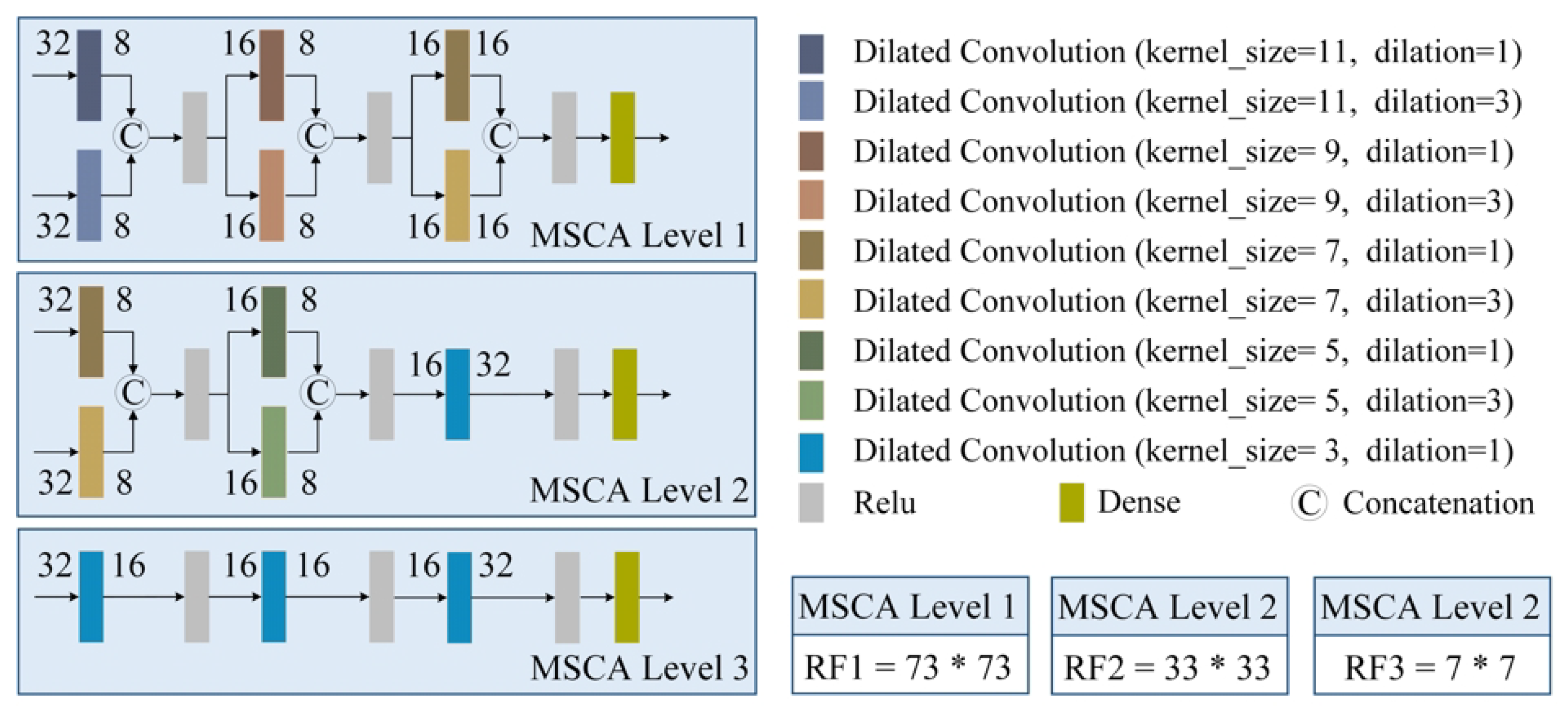
The detailed structure of the MSCA module is illustrated in Figure 2. A color-coding scheme is utilized in this figure to distinguish between convolutional operations with differing dilation rates. Specifically, the blue-colored boxes represent standard $3\times 3$ convolutions with dilation = 1, serving to preserve high-resolution spatial details.

As illustrated in Figure 2, MSCA1 employs a three-stage hierarchical architecture with progressively reduced kernel sizes ($11\times 11\to 9\times 9\to 7\times 7$). Each stage implements dual-path dilated convolutions, including dense sampling branch and sparse context branch. The dense sampling branch with dilation = 1 preserves high-frequency spatial details. The sparse context branch with dilation = 2 captures wide-area contextual patterns. Outputs from the two branches are fused via concatenation, activated by ReLU, and finally processed through a dense layer.

MSCA1 demonstrates distinctive capabilities for large-scale contextual understanding, particularly in extracting scene layouts and major object boundaries. This capability originates from the module’s multi-stage progression of large kernels with strategic dilation rates, forming an interconnected hierarchical processing chain. Specifically, the architecture enables exponential growth of the effective RF while maintaining key spatial details through residual pathways. MSCA2 employs a hybrid design similar to MSCA1, utilizing medium kernels ($7\times 7\to 5\times 5\to 3\times 3$) to optimally balance context capture and computational efficiency. This architecture uniquely combines dilated convolutions in $7\times 7$ and $5\times 5$ layers, enabling efficient medium-range context processing. The standard $3\times 3$ convolution effectively preserves fine spatial details that might be lost in dilated operations. Through this strategic combination, MSCA2 reduces computational overhead compared to MSV1 while retaining comparable performance. This makes MSCA2 particularly suitable for applications demanding both accuracy and processing efficiency. MSCA3 differs from MSCA1/MSCA2 by exclusively employing standard $3\times 3$ convolutions with a dilation rate of 1. This design preserves high spatial resolution to maintain fine details like textures and edges that MSCA1/MSCA2 might miss. MSCA3 focuses on small-scale details and local textures, avoiding the feature sparsity caused by dilated convolutions. Its lightweight standard convolutions ensure lower computational complexity and faster inference speeds. These characteristics enable MSCA3 to effectively refine fine-grained features like edges and textures after global context extraction.

The hierarchical design of MSCA achieves a global-to-local feature learning pipeline, where each level addresses a specific scale gap while synergizing with others. Dilated convolutions strategically expand the RF while minimizing computational overhead. Convolution and pooling are important operations in CNNs. However, downsampling in the encoder via convolution and pooling leads to a critical issue: the loss of detailed image information, which makes it difficult to reconstruct image features. For instance, with three pooling layers each using a stride of 2, any feature smaller than 8 pixels ($\left(2^3\right)$) in width/height will lose its information, making exact theoretical reconstruction impossible. In 2015, dilated convolution was first systematically defined and formally named in the deep learning literature, specifically for semantic segmentation tasks [22]. Dilated convolution is a novel convolutional approach proposed to address the issues of reduced image resolution and information loss caused by downsampling in image semantic segmentation. For an input feature map I and kernel K, the dilated convolution is defined as follows:

$$D{R}_r\left(p\right)=\sum _{s\in \Omega }I(p+r·s)·K\left(s\right)$$

(6)

where I is the feature map with size $H\times W\times C$, K is the kernel with size $k\times k$, p is the pixel location $(i,j)$, s is over kernel coordinates, $\Omega$ is the integration range with $\Omega =[0,k-1]\times [0,k-1]$, and r is dilation rate. When $r=1$, $D{R}_r$ is standard convolution. When $r>1$, $D{R}_r$ is the dilated convolution, where $r-1$ zeros are inserted between kernel elements.

By introducing a parameter known as dilation rate, dilated convolution enables a convolution kernel of the same size to obtain a larger RF. RF can be determined by kernel size and dilation rate, as shown in

$$R{F}_i=(R{F}_{i-1}-1)\times s_i+[(k_i-1)\times d_i+1]$$

(7)

where $R{F}_i$ is the RF at layer i ($R{F}_0=1$), $R{F}_{i-1}$ is the RF field from previous layer $i-1$, $s_i$ is the stride, $k_i$ is the kernel size, $d_i$ is the dilation rate. From Equation (7), we can see that the RF expands exponentially when using cascaded dilated convolutions. Specifically, the total RF size across n layers is given by the following:

$${RF}_{total}=1+\sum _{i=1}^n\left[(k_i-1)\times d_i\times \prod _{j=1}^{i-1}{s}_j\right]$$

(8)

where n is total number of layers, and ${\prod }_{j=1}^{i-1}{s}_j$ represents cumulative stride product from previous layers. RF determines a neuron’s spatial context, directly affecting a network’s ability to recognize patterns at different scales, including local textures and global structures. This is crucial for tasks like object detection, segmentation, and scene understanding.

Table 2. RF analysis for MSCA1.

Layer	Module	Kernel Size	Dilation	Internal RF	Cumulative RF
1	Conv11 (branch 1)	11	1	11	11
1	Conv11 (branch 2)	11	3	21	31
2	Conv9 (branch 1)	9	1	8	39
2	Conv9 (branch 2)	9	3	24	55
3	Conv7 (branch 1)	7	1	6	61
3	Conv7 (branch 2)	7	3	18	73

,

Table 3. RF analysis for MSCA2.

Layer	Module	Kernel Size	Dilation	Internal RF	Cumulative RF
1	Conv7 (branch 1)	7	1	7	7
1	Conv7 (branch 2)	7	3	19	19
2	Conv5 (branch 1)	5	1	4	23
2	Conv5 (branch 2)	5	3	12	31
3	Conv3 (d = 1)	3	1	2	33

,

Table 4. RF analysis for MSCA3.

Layer	Module	Kernel Size	Dilation	Internal RF	Cumulative RF
1	Conv31	3	1	3	3
2	Conv32	3	1	2	5
3	Conv33	3	1	2	7

and

Table 5. RF analysis of MSCA.

Module	Kernel Sequence	Dilation	Internal RF	Relative to Input
MSCA1	11-9-7	[1,3]-[1,3]-[1,3]	73	73
MSCA2	7-5-3	[1,3]-[1,3]-1	33	105
MSCA3	3-3-3	1-1-1	7	111

shows the RF expansion of dilated convolutions across varying dilation rates.

From Table 2, we can see that MSCA1 employs three branches with large kernel sizes, including $11\times 11$, $9\times 9$, and $7\times 7$. Each branch uses two parallel dilated convolutions with dilation rates of 1 and 3, respectively. Through sequential dilated convolutions, the RF of MSCA1 expands significantly to $73\times 73$, enabling each branch to capture multi-scale features. It uses high dilation rates to maintain wide coverage without requiring excessively large kernel sizes. MSCA1 enables efficient modeling of long-range dependencies and robust extraction of large-scale structures while balancing computational load through branch-wise parallel processing. MSCA2 has a moderate RF of $33\times 33$, as shown in Table 3, and it is smaller than that of MSCA1.

MSCA2 strategically combines dilated and standard convolutions. It uses dual-branch dilation with dilation rates 1 and 3 only in its initial $7\times 7$ layer. These are followed by smaller kernels: 5 × 5 with dilation and 3 × 3 without dilation. This hybrid approach focuses on mid-scale feature harmonization. It reduces computational complexity compared to MSV1 while still retaining multi-scale sensitivity. It balances detail preservation and contextual integration. This makes it suitable for capturing object-level features without sacrificing spatial resolution.

MSCA3 focuses on pixel-level precision, enhancing texture recovery and edge sharpness. It uses only standard $3\times 3$ convolutions with a dilation rate of 1 across three sequential layers, each having an internal receptive field of $7\times 7$ as shown in Table 4. This dilation-free design emphasizes optimizing local details by maintaining high feature density and minimizing spatial sparsity. Its simplicity ensures computational efficiency, avoids dilation artifacts, and makes it effective for refining fine-grained structures in shallow network stages. The MSCA architecture employs a hierarchical cascade of three specialized modules, with their RF decreasing progressively to enable multi-scale feature extraction. Through the cascaded framework, MSCA achieves progressive RF expansion up to 111 pixels, following the sequence: MSCA1 (73 RF) → MSCA2 (105 RF) → MSCA3 (111 RF).

This design adopts a coarse-to-fine processing strategy: early stages capture broad structural patterns, while later stages refine local details. The realization of this coarse-to-fine strategy is achieved through multi-scale receptive field expansion using dilated convolutions. We connect theoretical analysis with experimental proof. We use both mathematical formulas and visual results. Figure 3 shows how we expand the receptive field from RF = 1 to RF = 11 using dilated convolutions. Figure 4 confirms this works in practice. It shows that different receptive fields capture different cloud features. Small ones get local textures. Medium ones find cloud edges. Large ones see the overall cloud layout. This combination gives solid theoretical support through math. It also provides clear visual proof through experiments. Together, they make the case for our MSCA module design stronger.

MSCA enables comprehensive feature representation while maintaining computational efficiency. The features and quantitative contributions of the MSCA architecture are shown in

Table 6. Features of the MSCA. ↑ and ↓ mean that the better methods should achieve a higher/lower score of this metric.

Aspect	MSCA
Specialization	Multi-scale context capture.
Performance Impact	Improves PSNR ↑ by 0.361 dB, reduces SAM ↓ by 0.147 and reduces ERGAS ↓ by 0.004.
Parameter Reduction	6% decrease.
RF Expansion	RF Expansion of $111\times 111$.
Representation	Hierarchical multi-scale feature integration.

.

3.5. Refined Residual Blocks

The RRB design is grounded in boundary protection and residual calibration theories. It uses reflection padding to mirror edge pixels, preserving boundary integrity and avoiding artificial zero-value distortion. The SiLU activation function provides smoother gradients than ReLU, thereby enhancing training stability. A scaling factor was applied to the main branch to balance the weights between branches, and a $1\times 1$ convolution calibrates the residual branch for effective feature fusion.

The RRB is a Refined Residual Block that uses reflection padding to reduce boundary artifacts. SiLU (Swish) activation $SiLU\left(x\right)=x·\sigma \left(x\right)$ was used for better gradient flow and non-linearity. The RRB employs residual adjustment ($1\times 1$ convolution) to calibrate the residual branch and applies a scaling factor (0.1) to the second convolution’s output to stabilize training. The forward pass can be expressed as follows:

$$\mathrm{output}=\underset{Scaled feature transform}{\underbrace{\mathcal{F}\left(x\right)\times 0.1}}+\underset{Residual branch}{\underbrace{\mathcal{G}\left(x\right)}}$$

(9)

where $\mathcal{F}$ represents the two convolutional layers with SiLU activation, and $\mathcal{G}$ denotes the 1 × 1 convolution for residual adjustment. This design enhances feature integration, while the scaling factor prevents the residual branch from overwhelming the main branch. The features and quantitative contributions of the MSCA architecture are shown in

Table 7. Features of the RRB. ↑ and ↓ mean that the better methods should achieve a higher/lower score of this metric.

Aspect	RRB
Specialization	Boundary artifact reduction and residual branch balance optimization.
Performance Impact	Improves PSNR ↑ by 0.753 dB, SSIM ↑ by 0.001, reduces SAM ↓ by 0.147 and reduces ERGAS ↓ by 0.009.
Representation	Edge-preserved.

.

3.6. Iterative Feature Refinement

The design of this module draws on dense connection theory and progressive optimization principles. Through dense cross-stage connections, the output of each stage is concatenated with the original input, allowing the reuse of valuable early-stage features and minimizing error propagation. The coarse-to-fine refinement approach aligns well with the thin cloud removal workflow: it starts by eliminating large-area clouds, proceeds to adjust medium-scale structures, and ultimately refines the details.

The IFR module uses an iterative processing pipeline with dense, multi-scale connections. The processing flow consists of three key operations, shown in Equation (10):

Input feature channels are split and initially processed through DBAA. The features are passed through MSCA blocks (MSCA1, MSCA2, MSCA3) The stage outputs are concatenated with the original input and processed through dense residual blocks.

$$\begin{array}{ccc}\hfill Input\stackrel{Conv}{\to }& \hfill Split\stackrel{Stage1:DBAA+MSCA1}{\to }Concat\stackrel{Dense}{\to }\hfill & \hfill \\ \hfill & \hfill Split\stackrel{Stage2:DBAA+MSCA2}{\to }Concat\stackrel{Dense}{\to }\hfill & \hfill \\ \hfill & \hfill Split\stackrel{Stage3:DBAA+MSCA3}{\to }Concat\stackrel{Dense}{\to }\hfill & Output,Input\stackrel{Dense}{\to }\hfill \end{array}$$

(10)

This architecture is based on three ideas: multi-stage coarse-to-fine refinement, dense connections with residual concatenation for robust information flow, and shared attention mechanisms for parameter efficiency. The features of the IFR architecture are shown in

Table 8. Features of the IFR. ↑ and ↓ mean the better methods should achieve a higher/lower score of this metric.

Aspect	IFR
Specialization	Progressive coarse-to-fine feature refinement and residual propagation error suppression.
Performance Impact	Improves PSNR ↑ by 0.236 dB, reduces SAM ↓ by 0.16 and reduces ERGAS ↓ by 0.007.
Representation	Dense cross-stage integrated feature representation with iterative enhancement.

.

4. Results

In this section, we present some experimental results. We first describe the implementation details in Section 4.1 and then the datasets in Section 4.2 Next, Section 4.3 evaluates the performance of the proposed algorithm qualitatively and quantitatively by comparison with the state-of-the-art dehazing methods, respectively. Finally, we show the ablation study and the network configurationin Section 4.4.

4.1. Implementation Details

As shown in Figure 1, the proposed network contains three levels in the encoder. A composite loss function, denoted as ${\mathcal{L}}_{\mathrm{total}}$, is employed to guide the training process. It integrates the Mean Squared Error (MSE) loss, perceptual loss, and color loss, formulated as follows:

$$\mathcal{L}\mathrm{total}=\mathcal{L}\mathrm{mse}+{\displaystyle \frac{\mathcal{L}\mathrm{vgg}}{(\mathcal{L}\mathrm{vgg}/\mathcal{L}\mathrm{mse})}}+{\displaystyle \frac{\mathcal{L}\mathrm{color}}{(\mathcal{L}\mathrm{color}/\mathcal{L}\mathrm{mse})}}$$

(11)

Here, $\mathcal{L}\mathrm{mse}$ denotes the MSE loss, $\mathcal{L}\mathrm{vgg}$ is the VGG-based perceptual loss, and $\mathcal{L}\mathrm{color}$ is the color-consistency loss. Critically, the gradient flow through the ratio terms $(\mathcal{L}\mathrm{vgg}/\mathcal{L}\mathrm{mse})$ and $(\mathcal{L}\mathrm{color}/{\mathcal{L}}_{\mathrm{mse}})$ is stopped during backpropagation, ensuring that all three loss components contribute directly to the gradient while maintaining adaptive balancing throughout the optimization process.

The initial learning rate is 0.0001 with a weight decay of 0.0005, and a cosine annealing learning rate scheduler is applied. The entire training process is optimized by the ADAM [23] solver with $\beta 1=0.9$ and $\beta 2=0.999$ with a batch size of 4. Our model is trained for 50 epochs with an initial learning rate of 0.0001 and a weight decay of 0.0005. To evaluate the performance of our method, we adopt the PSNR, SSIM, spectral angle mapper (SAM) and relative dimensionless global error in synthesis (ERGAS) as the evaluation metrics. PSNR and SSIM are better when their values are larger, as they indicate higher similarity between the generated image and the reference image. In contrast, SAM and ERGAS are better when smaller, reflecting lower spectral discrepancy and global synthesis error. The code of PMSAF-Net is modified based on PM-LSMN. All the experiments are conducted on NVIDIA GeForce RTX 3090 Ti graphics processing unit (GPU) (NVIDIA Corporation, Santa Clara, CA, USA).

4.2. Datasets

We use the RICE1, RICE2, T-cloud, and WHUS2-CR datasets for evaluation. These multi-source datasets provide a robust testbed for evaluating the model’s cross-platform generalization capability. The RICE dataset provides a cross-source validation challenge: RICE1 contains optical images sourced via Google Earth, while RICE2 is based on Landsat 8 imagery with thick clouds. The T-cloud dataset offers a multispectral Landsat 8 benchmark, and WHUS2-CR introduces the distinct spectral profile of Sentinel-2A across diverse regions, collectively forming a comprehensive evaluation framework.

We adopt the cross-source RICE [7] to train and evaluate our model. The RICE dataset is composed of two subsets: RICE1 and RICE2. RICE1 contains 500 pairs of $512\times 512$ images, sourced from Google Earth. RICE2 comprises 450 pairs of $512\times 512$ images, derived from the Landsat 8 OLI/TIRS dataset. Specifically, its image pairs are selected from images captured at the same location within a 15-day window to ensure consistency in underlying ground features. T-cloud [24] dataset comprises 2939 pairs of $256\times 256$ images, sourced from Landsat 8 multispectral imagery. We randomly select 400 pairs for training and 100 pairs for testing. WHUS2-CR is a cloud removal evaluation dataset with cloudy/cloud-free paired Sentinel-2A images from the Copernicus Open Access Hub, selected under the conditions of: (1) wide distribution, (2) all-season coverage [25].

Sentinel-2A is a high-resolution multi-spectral imaging satellite that carries a multi-spectral imager (MSI) covering 13 spectral bands in the visible, near infrared, and shortwave infrared [25]. Band 2 represents the red band, with a central wavelength of 0.490 µm, a bandwidth of 98 nm, and a spatial resolution of 10 m. Band 3 represents the green band, with a central wavelength of 0.560 µm, a bandwidth of 45 nm, and a spatial resolution of 10 m. Band 4 represents the blue band, with a central wavelength of 0.665 µm, a bandwidth of 38 nm, and a spatial resolution of 10 m. In our experiment, We select Band 2/3/4 images from two regions, that is, Ukraine with Urban Land Cover, Australia with Urban. For each region, we randomly select 400 pairs for training and 100 pairs for testing. The images pairs are resized to $512\times 512$.

4.3. Comparisons with State-of-the-Art Methods

In this section, our method is evaluated qualitatively and quantitatively against the state-of-the-art methods based on the hand-crafted priors DCP [26] and deep convolutional neural networks (AOD-Net [27], CloudGAN [28], McGANs [29], CycleGAN [30], DC-GAN-CL [31], Vanilla GAN [32], U-net GAN [32], MAE-CG [33], PM-LSMN [11]). We evaluate PMSAF-Net against several representative cloud removal methods. These methods span different technical paradigms. They include the physics-based classical baseline DCP and efficient CNN architectures such as the lightweight AOD-Net. Our primary contemporary baseline is PM-LSMN, which is specifically designed for thin cloud removal. We also compare with popular GAN-based approaches, including the standard unpaired training framework CycleGAN. This category contains recent improvements like DC-GAN-CL and U-net GAN, along with earlier variants such as CloudGAN and McGANs. Additionally, we include the recent attention-enhanced method MAE-CG, which incorporates multi-attention mechanisms. This selection encompasses both established benchmarks and the latest advances, ensuring a comprehensive performance comparison.

To demonstrate the effectiveness of our method, we conducted training and qualitative evaluations on the RICE1, RICE2, T-Cloud, and WHUS2 datasets in this section. The results indicate that our method achieves performance comparable to other methods. First, we quantitatively compare our method with the other methods on the RICE1 dataset, as shown in

Table 9. Quantitative evaluations on RICE1. ↑ and ↓ mean that the better methods should achieve a higher/lower score of this metric.

Methods	PSNR ↑	SSIM ↑	SAM ↓	ERGAS ↓
DCP	19.109	0.803	9.383	0.798
CycleGAN	26.888	0.819	3.342	0.629
AOD-Net	20.043	0.832	8.114	0.557
McGANs	22.049	0.616	4.219	0.624
CloudGAN	21.515	0.699	13.863	1.072
DC-GAN-CL	22.049	0.616	7.317	0.472
Vanilla GAN	21.090	0.692	7.509	0.487
U-net GAN	26.232	0.794	6.229	0.408
MAE-CG	24.800	0.862	6.598	0.430
PM-LSMN	25.939	0.927	5.73	0.41
Ours	27.258	0.930	5.423	0.39

. For the PSNR metric, our method ranks first with a value of 27.258, followed by CycleGAN (26.888) in second place and PM-LSMN (25.939) in third. In terms of SSIM, our method achieves the highest value of 0.930. Regarding the SAM metric, our method secures a respectable third place with a value of 5.423. For the ERGAS metric, our method attains the lowest (best) score of 0.39 among all methods, outperforming the second-ranked PM-LSMN (0.41) and other competitors. It can be seen that our method achieves the top rank in three out of the four evaluation metrics (PSNR, SSIM, ERGAS) and a competitive third rank in SAM. This shows that our method achieves comparable results with the other methods.

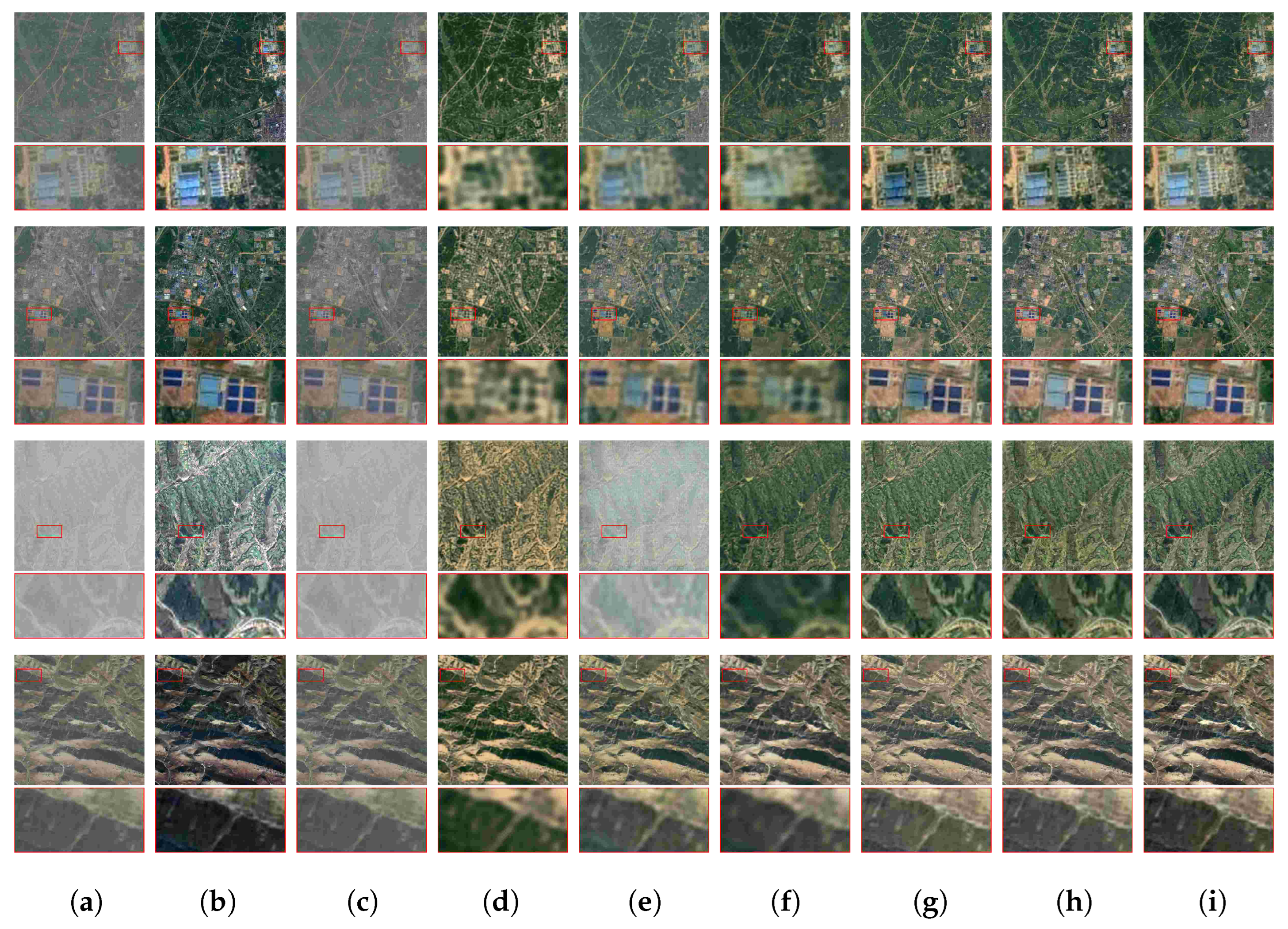
Qualitative results on RICE1 are shown in Figure 5. Our method effectively removes cloud haze while preserving fine details and maintaining natural, vivid colors. The resulting images are visually clear and closely resemble the ground truth shown in Figure 5i. In the magnified views of the first and second rows of Figure 5h, the color of the blue lake closely matches that of the corresponding ground truth.

Figure 6 shows the pixel-wise mean absolute error (MAE) between different methods and the ground truth. The error maps clearly show that our method achieves the lowest reconstruction error. This is visible from the dominant blue colors in subfigure (d), which represent small errors. In comparison, CloudGAN (b) and PM-LSMN (c) show more warm-colored areas. These warm colors mean larger errors remain. The input image (a) has the highest errors, especially where clouds are present. These visual comparisons confirm that our approach better preserves original scene details while effectively eliminating cloud interference.

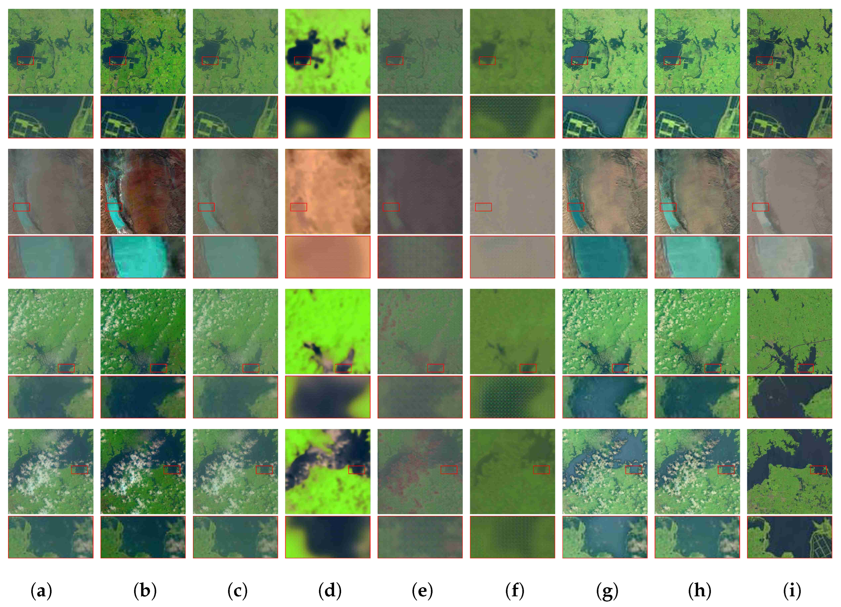
Unlike RICE1, the RICE2 dataset contains thick cloud layers that completely obscure the underlying image content. Recovering such heavily occluded details is inherently challenging and typically requires additional input sources, as the algorithm cannot reconstruct information that is entirely absent. Despite this limitation, which precludes full reconstruction in heavily occluded areas, our experiments demonstrate that our method maintains robust performance. As shown in

Table 10. Quantitative evaluations on RICE2. ↑ and ↓ mean that the better methods should achieve a higher/lower score of this metric.

Methods	PSNR ↑	SSIM ↑	SAM ↓	ERGAS ↓
DCP	17.735	0.599	21.037	1.275
CycleGAN	27.794	0.823	4.248	0.871
AOD-Net	17.755	0.486	33.09	3.177
McGANs	19.403	0.357	6.839	0.979
CloudGAN	24.814	0.764	14.425	2.77
DC-GAN-CL	19.433	0.356	8.427	0.983
Vanilla GAN	20.102	0.651	7.312	0.862
MAE-CG	24.207	0.843	7.293	0.728
U-net GAN	25.305	0.768	8.427	0.657
PM-LSMN	28.144	0.87	6.183	0.516
Ours	28.855	0.87	5.689	0.476

, it achieves superior results on metrics that assess overall fidelity (PSNR, SSIM, ERGAS). Visually, as illustrated in Figure 7, our approach retains better color fidelity and detail preservation with fewer artifacts compared to other methods, which often exhibit severe color distortion.

For PSNR, our method ranks first with 28.855, followed by PM-LSMN (28.144) in second and CycleGAN (27.794) in third. For SSIM, our method reaches 0.87, tying with PM-LSMN for the highest score. Both outperform competitors like CycleGAN (0.823) and CloudGAN (0.764). For SAM, our method takes second place with 5.689; CycleGAN (4.248) is first, and PM-LSMN (6.183) ranks third. For ERGAS, our method obtains the lowest score of 0.476 among all methods. These results show that our method achieves the top or joint-top rank in three out of the four evaluation metrics (first in PSNR and ERGAS, joint-first in SSIM) and a highly competitive second place in SAM.

Figure 7 shows results on the challenging RICE2 dataset with thick clouds. While the heavy occlusion poses difficulties, our method retains better color fidelity and detail preservation compared to others, which exhibit severe color distortion or artifacts. Our method removes thin clouds while retaining relatively fidelity in both original color tone and spatial details. The baseline method of PM-LSMN exhibits a color discrepancy along the lake boundaries, whereas our proposed approach effectively mitigates this issue without introducing visible color artifacts.

While the quantitative results on RICE2 appear superior to those on RICE1, this should be interpreted in the context of fundamental dataset differences. Performance variation stems from the inherent characteristics of each dataset. RICE1 contains high-resolution details that are difficult to recover perfectly. This challenge often leads to a lower PSNR score. In contrast, RICE2 features thick clouds that frequently obscure the underlying scene. As a result, the task shifts from thin-cloud removal to content inpainting. Our model addresses this by generating semantically plausible content in the missing regions. This approach can result in higher PSNR when the generated content aligns well with the reference. Therefore, the superior performance on RICE2 reflects the model’s strong generative capability rather than better thick-cloud removal. The core challenge remains the recovery of subtle details in RICE1’s thin cloud scenarios.

Table 11. Quantitative evaluations on T-cloud. ↑ and ↓ mean that the better methods should achieve a higher/lower score of this metric.

Methods	PSNR ↑	SSIM ↑	SAM ↓	ERGAS ↓
DCP	19.109	0.652	16.123	0.907
CycleGAN	23.719	0.799	5.490	0.728
AOD-Net	20.008	0.716	14.465	0.768
McGANs	22.424	0.553	6.998	0.840
CloudGAN	17.057	0.741	14.303	0.590
DC-GAN-CL	22.45	0.552	8.59	0.844
Vanilla GAN	21.92	0.653	8.38	0.820
U-net GAN	23.59	0.770	7.69	0.678
MAE-CG	22.40	0.830	8.09	0.750
PM-LSMN	23.791	0.848	9.292	0.664
Ours	24.164	0.846	9.007	0.612

presents quantitative results on the T-cloud dataset. For PSNR, our method ranks first with 24.164, followed by PM-LSMN (23.791) in second and CycleGAN (23.719) in third. For SSIM, PM-LSMN achieves the highest score of 0.848, while our method closely follows with 0.846, securing second place, and MAE-CG ranks third with 0.830. For SAM, CycleGAN obtains the best score of 5.490, followed by McGANs (6.998) in second and U-net GAN (7.69) in third, while our method ranks seventh with 9.007. For ERGAS, CloudGAN achieves the lowest score of 0.590, with our method ranking third at 0.612, following AOD-Net (0.768). These results demonstrate that our method achieves the top rank in one metric (PSNR), competitive second-place rankings in two metrics (SSIM and SAM), and a respectable third place in ERGAS.

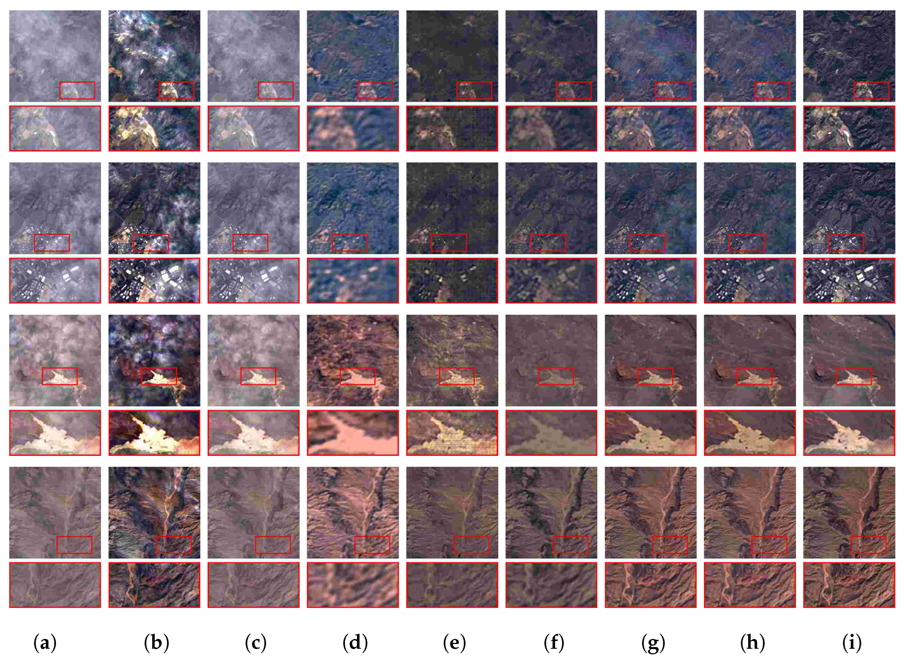
On the T-cloud dataset, which contains diverse cloud types, our method demonstrates more effective cloud removal compared to PM-LSMN and other approaches, with less residual cloud cover as shown in Figure 8. Our method is similar to PM-LSMN but demonstrates a more effective capacity for cloud removal. In the first and second rows, the output images in Figure 8h contain less cloud cover than those from PM-LSMN in Figure 8g.

The T-cloud dataset contains diverse cloud types, ranging from thin, semi-transparent clouds to thick, complex coverings. Without multi-modal inputs, the experiments show limited performance in these scenarios. Nevertheless, our approach maintains moderate overall visual quality in terms of color accuracy, detail clarity, and cloud removal.

WHUS2-CR consists of real Sentinel-2A images. For our experiments, the Blue (B2), Green (B3), and Red (B4) bands were concatenated to form true color composited image. We conducted four tests targeting four regions: Test 1, an urban area in Ukraine; Test 2, an urban area in Australia. To demonstrate the visual characteristics of individual bands, we present the following for Test 1: the standard RGB composite, and the separate grayscale images from Band 2 (Blue), Band 3 (Green), and Band 4 (Red).

Table 12. Quantitative evaluations on WHUS2 test1. ↑ and ↓ mean that the better methods should achieve a higher/lower score of this metric.

Methods	PSNR ↑	SSIM ↑	SAM ↓	ERGAS ↓
DCP	19.429	0.629	23.280	1.826
CycleGAN	22.736	0.702	8.726	0.168
AOD-Net	17.758	0.544	29.676	2.177
McGANs	21.541	0.672	7.901	1.074
CloudGAN	16.461	0.705	13.458	0.429
DC-GAN-CL	21.571	0.671	9.491	1.077
Vanilla GAN	21.241	0.752	9.101	1.054
U-net GAN	22.536	0.732	10.526	0.857
MAE-CG	21.336	0.762	10.826	0.997
PM-LSMN	21.768	0.764	16.621	1.257
Ours	23.084	0.789	15.451	0.967

presents quantitative results on the WHUS2 test1 dataset. For PSNR, our method ranks first with 23.084, followed by CycleGAN (22.736) in second and U-net GAN (22.536) in third. For SSIM, our method achieves the highest score of 0.789, while PM-LSMN closely follows with 0.764 in second place and MAE-CG (0.762) in third. For SAM, McGANs obtains the best score of 7.901, with CycleGAN (8.726) ranking second and Vanilla GAN (9.101) in third, while our method ranks eighth with 15.451. For ERGAS, CycleGAN attains the lowest score of 0.168, followed by CloudGAN (0.429) in second and U-net GAN (0.857) in third, while our method ranks fifth with 0.967. These results demonstrate that our method achieves the top rank in two metrics (PSNR and SSIM) while maintaining competitive performance in the remaining metrics.

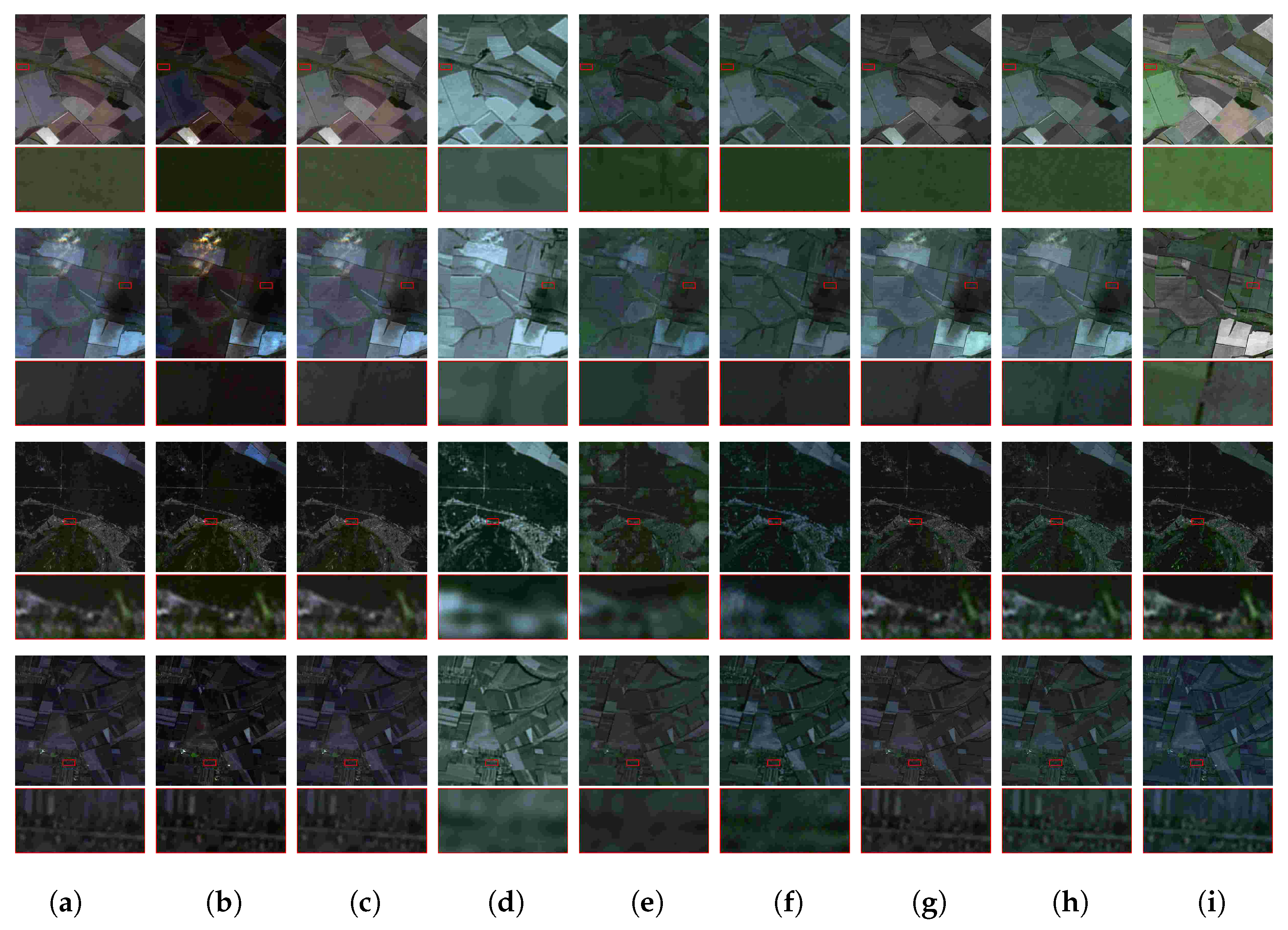
For the real Sentinel-2A images in WHUS2-CR (Figure 9), our method and PM-LSMN show comparable cloud removal, but our results exhibit more accurate color representation, closer to the ground truth. The WHUS2 test1 dataset contains diverse scenes with varying cloud conditions. Our approach maintains better visual quality in terms of color accuracy, detail clarity, and cloud removal compared to other methods, producing results that are more consistent with the ground truth.

Our proposed PMSAF-Net achieves state-of-the-art or comparable performance across all benchmark datasets with merely 0.32 M trainable parameters, demonstrating its superior accuracy-efficiency trade-off for multi-platform deployment. Qualitative evaluations reveal that the method effectively removes thin clouds while preserving spectral continuity and color consistency.

4.4. Ablation Study and Configuration Analysis

Based on our model, we construct 6 variants with different component combinations: (a) Variant model A is the baseline PM-LSMN model. (b) Variant model B adopts the DBAA module. (c) Variant model C adopts the RRB block. (d) Variant model D adopts the MSCA module. (e) Variant model E adopts the IFR modules. (f) Proposed model F adopts all the introduced modules (DBAA, RRB, MSCA, and IFR). In

Table 13. Quantitative comparison for the ablation study on RICE1. Variant model A is the baseline PM-LSMN model. Variant model B adopts the DBAA module. Variant model C adopts the RRB block. Variant model D adopts the MSCA module. Variant model E adopts the IFR modules. Variant model F is the proposed model, which adopts the DBAA, RRB, MSCA and IFR modules. All the methods are trained and evaluated on the RICE1. The checkmark denotes the adoption of the corresponding component in each model’s architecture. ↑ and ↓ mean that the better methods should achieve a higher/lower score of this metric.

Variant Models	A	B	C	D	E	F
DBAA		✓				✓
RRB			✓			✓
MSCA				✓		✓
IFR					✓	✓
PSNR ↑	25.939	26.802	26.692	26.300	26.175	27.258
		(+3.33%)	(+2.90%)	(+1.39%)	(+0.91%)	(+5.08%)
SSIM ↑	0.927	0.911	0.928	0.909	0.913	0.930
		(−1.73%)	(+0.11%)	(−1.94%)	(−1.51%)	(+0.32%)
SAM ↓	5.730	5.583	5.439	5.600	5.654	5.423
		(−2.57%)	(−5.08%)	(−2.27%)	(−1.33%)	(−5.36%)
ERGAS ↓	0.410	0.392	0.401	0.406	0.404	0.390
		(−4.39%)	(−2.20%)	(−0.98%)	(−1.46%)	(−4.88%)
Parameters (M) ↓	0.33	0.31	0.41	0.31	0.40	0.32
		(−6.06%)	(+24.24%)	(−6.06%)	(+21.21%)	(−3.03%)

, the models B, C, D and E achieve improvement gains in PSNR of 0.863 dB, 0.753 dB, 0.361 dB and 0.236 dB, respectively, compared to model A, demonstrating the effectiveness of the proposed individual modules. Our proposed model F achieves the best performance with PSNR of 27.258 dB and SSIM of 0.930, outperforming all variant models across multiple metrics. Furthermore, model F achieves the best scores in SAM (5.423) and ERGAS (0.390), demonstrating comprehensive performance improvements. With approximately 0.32 M parameters, model F maintains a compact model size comparable to the baseline model A (0.33 M parameters). Therefore, the introduced DBAA, RRB, MSCA, and IFR modules collectively enable our model to achieve better performance while maintaining computational efficiency.

4.4.1. Effectiveness of Proposed Modules

All values of Variants B-F are formatted as “measured value (relative baseline change rate%)”, where the change rate is calculated as [(Variant Value-Baseline Value)/Baseline Value] × 100. For positive indicators (PSNR, SSIM; higher is better), a positive change rate denotes improvement. For negative indicators (SAM, ERGAS, Parameters; lower is better), a negative change rate denotes optimization. All ablation experiments were conducted on the RICE1 dataset. The ablation study reveals distinct contributions from each module:

DBAA enhances performance by increasing PSNR by 3.33% through the separate optimization of spatial and channel attention. This approach significantly reduces computational redundancy while improving feature extraction efficiency. RRB achieves superior spectral preservation, reducing SAM by 5.08%, through the use of reflection padding and residual calibration. This effectively minimizes boundary artifacts, ensuring more accurate spectral information retention. MSCA contributes to ERGAS improvement by 0.98% by expanding the receptive field to 111 × 111 through hierarchical dilated convolutions. This enables better global context capture, crucial for handling complex cloud distributions. IFR provides moderate but consistent improvements across all metrics through dense cross-stage connections. This ensures progressive feature refinement and error reduction, enhancing overall image quality. The integrated model (F) achieves synergistic performance, with a 5.08% improvement in PSNR and a 5.36% reduction in SAM, while maintaining a compact parameter size of 0.32 M, slightly smaller than the baseline.

We conducted ablation studies on the RICE1 dataset to evaluate each component’s contribution. Using a single benchmark allows for a controlled comparison, isolating the effect of each module without the added complexity of multiple datasets. A comprehensive ablation study has been conducted on the RICE2 dataset to complement the analysis on RICE1. The results, summarized in Table 13 and

Table 14. Quantitative comparison for the ablation study on RICE2. Variant model A is the baseline PM-LSMN model. Variant model B adopts the DBAA module. Variant model C adopts the RRB block. Variant model D adopts the MSCA module. Variant model E adopts the IFR modules. Variant model F is the proposed model, which adopts the DBAA, RRB, MSCA and IFR modules. All the methods are trained and evaluated on the RICE2. The checkmark denotes the adoption of the corresponding component in each model’s architecture. ↑ and ↓ mean that the better methods should achieve a higher/lower score of this metric.

Variant Models	A	B	C	D	E	F
DBAA		✓				✓
RRB			✓			✓
MSCA				✓		✓
IFR					✓	✓
PSNR ↑	28.144	28.462	28.713	28.832	28.395	28.855
		(+1.13%)	(+2.02%)	(+2.44%)	(+0.89%)	(+2.53%)
SSIM ↑	0.871	0.871	0.872	0.871	0.872	0.872
		(0.00%)	(+0.11%)	(0.00%)	(+0.11%)	(+0.11%)
SAM ↓	6.183	5.924	5.781	5.712	6.052	5.689
		(−4.19%)	(−6.50%)	(−7.62%)	(−2.12%)	(−7.99%)
ERGAS ↓	0.513	0.498	0.483	0.478	0.508	0.476
		(−2.92%)	(−5.85%)	(−6.82%)	(−0.97%)	(−7.21%)
Parameters (M) ↓	0.33	0.31	0.41	0.31	0.40	0.32
		(−6.06%)	(+24.24%)	(−6.06%)	(+21.21%)	(−3.03%)

, confirm that the contributions of the DBAA, RRB, MSCA, and IFR modules are consistent across both datasets. This demonstrates the general effectiveness of the proposed architectural components under varying cloud scenarios.

To systematically evaluate the contribution of each component, we first conducted an ablation study on the RICE1 dataset. This study provided a controlled benchmark for isolating module effects. To further verify the generalizability of these findings, this study was extended to the RICE2 dataset. This dataset presents different cloud characteristics.

As shown in Table 14, the results demonstrate consistent performance improvements from the DBAA, RRB, MSCA, and IFR modules on RICE2 dataset, confirming their robustness and universal effectiveness under varying conditions.

These results demonstrate the value of each module within our architecture. Furthermore, the performance of our full model across all four datasets shows that these benefits generalize well. Our complete model achieves competitive results on RICE1, RICE2, T-cloud, and WHUS2-CR, which have different cloud types and sensors. This consistent performance confirms that our architectural improvements are effective across diverse real-world conditions.

4.4.2. Study of the Network Configuration

We evaluate our method on RICE1 under different network configurations, shown in

Table 15. Effects of Network Configuration. CC represents the Channel Count, KS represents the Kernel Size, and DR represents the Dilation Rate. All model variants are trained and evaluated on the RICE1 dataset. ↑ and ↓ mean that the better methods should achieve a higher/lower score of this metric.

Category	Configuration	PSNR ↑	SSIM ↑	SAM ↓	ERGAS ↓	Param (M) ↓	FLOPs (G) ↓	Training Time (h) ↓	Inference Time (s) ↓
CC	Baseline (64)	27.094	0.928	5.462	0.391	0.32	190.34	4.07	0.10
	Half-channels (32)	26.258	0.924	5.159	0.404	0.08	47.82	3.71	0.04
	Quarter-channels (16)	22.526	0.892	6.853	0.497	0.02	12.80	2.97	0.02
KS	Multi-scale (11/9/7/5/3)	27.094	0.928	5.462	0.391	0.32	190.34	4.07	0.10
	Small only (5/3)	26.473	0.925	5.586	0.404	0.23	144.17	3.47	0.03
	Middle only (9/7)	26.460	0.924	5.492	0.404	0.30	181.75	3.95	0.04
	Large only (11/9)	27.210	0.930	5.470	0.390	0.48	275.16	4.53	0.10
DR	Dense (1,1)	26.589	0.926	5.481	0.404	0.32	190.34	4.06	0.09
	Moderate (1,2)	27.094	0.928	5.462	0.391	0.32	190.34	4.07	0.09
	Increased (1,3)	27.258	0.930	5.423	0.390	0.32	190.34	4.02	0.10
	Large (1,4)	27.147	0.929	5.344	0.385	0.32	190.34	4.05	0.10
	Sparse (1,5)	26.831	0.928	5.558	0.396	0.32	190.34	4.06	0.11

. Considering the trade-off between model performance and hardware efficiency, we selected the configuration that offers the best balance. In terms of Channel Count (CC), the baseline (64 channels) is chosen as it provides superior performance (PSNR: 27.094) with acceptable parameters, while half (0.08 M) and quarter (0.02 M) channels lead to significant performance drops. For the Kernel Size (KS), the multi-scale configuration is selected for its robust performance across metrics. For the Dilation Rate (DR), the setting d = (1,3) is adopted because it achieves the highest PSNR (27.258) and excellent SSIM (0.930) without increasing the parameter counts. This combination ensures optimal performance while maintaining computational efficiency.

4.5. Benchmark Tests on Edge Computing Platforms

To validate the practical deployment capability of PMSAF-Net, we performed benchmark tests on a typical edge device. The following section details the setup and results.

We used a development board with a Rockchip RK3588 SoC (Rockchip Electronics Co., Ltd., Fuzhou, Fujian, China). This processor is designed for edge AI applications. The model was optimized with the official RKNN toolkit (v2.3.2). The input tensor shape was set to (1, 512, 512, 3). All tests ran under normal conditions without active cooling. The results confirm the model’s efficiency in resource-limited settings. Key metrics are listed in

Table 16. Edge deployment performance metrics on RK3588.

Metric	Value
Inference Time (ms)	508.68
Total System Memory (GB)	8.31
Memory Used Before Inference (GB)	0.54
Memory Used After Inference (GB)	0.55
Chip Temperature (°C)	33.307

.

The model achieved a single-image inference time of 508.68 ms, demonstrating its capability for near-real-time processing on edge hardware. This sub-second latency is suitable for applications such as onboard satellite or UAV image processing. Prior to execution, the system reported 0.54 GB of memory in use, leaving 7.44 GB free, which corresponded to a minimal memory utilization rate of 10.4%. This initial state indicates a low system load, establishing a clean baseline for measurement. Memory usage was closely monitored. Before inference, the system used 0.54 GB of memory. After inference, it used 0.55 GB. The increase was only 0.01 GB (10 MB). This shows a very low memory footprint.

The key finding from this data is the model’s exceptionally low dynamic memory footprint. The inference process resulted in an incremental memory consumption of only approximately 0.01 GB (10 MB). This negligible increase in resource demand powerfully validates the model’s lightweight architecture and its suitability for deployment on memory-sensitive edge devices without causing significant resource contention. The chip temperature remained stable at 33.3 °C before and after inference. This minimal thermal fluctuation indicates low power draw and operational stability, which is critical for always-on or battery-powered edge devices. The benchmark results substantiate that PMSAF-Net meets the critical requirements for edge deployment. It successfully balances computational accuracy with low latency, a minimal memory footprint, and stable power characteristics. This balance fulfills the core design objective of enabling effective multi-platform deployment. These performance characteristics directly align with the constraints of target edge platforms. With only 0.32 M parameters and a 10 MB memory footprint, PMSAF-Net operates well within the limits of typical deployment scenarios. For instance, it is compatible with nano-satellites such as CubeSats, which typically have memory constraints under 2 GB. The model also suits drone processors like the NVIDIA Jetson series, designed for 5–15 W power budgets. This validates PMSAF-Net’s practical deployment capability across various resource-constrained multi-platform scenarios.

5. Discussion

Our study presents PMSAF-Net, a lightweight network that addresses the hardware constraints of multi-platform deployment. From the perspective of prior studies, existing methods face inherent trade-offs: physics-based approaches fail in complex scenarios; GAN-based methods have high computational complexity; and Transformer-based models require large GPU memory. These challenges make practical deployment on multi-platform hardware difficult. Our ablation studies show that each module addresses specific limitations by adapting existing techniques: DBAA is based on parallel attention, and MSCA builds on dilated convolutions. Their combined integration, rather than single breakthroughs, enables good performance. Computational efficiency is crucial for practical deployment. Our model, PMSAF-Net, maintains strong performance with very few parameters (0.32 M) and low FLOPs (190.34 G). It also infers rapidly (0.0973 s per image). This balance of low cost and high speed makes it ideal for resource-limited platforms.

Collectively, they enable PMSAF-Net to achieve superior results while maintaining a compact model size of only 0.32 M parameters, underscoring its suitability for resource-constrained scenarios like onboard satellites and drone real-time monitoring. While PMSAF-Net achieves top ranks in PSNR and SSIM on the WHUS2 dataset, its lower rankings in SAM (spectral angle matching) and ERGAS indicate a relative challenge in spectral fidelity. This inconsistency may stem from the complex spectral characteristics of Sentinel-2A imagery. The model may prioritize spatial detail and structural similarity (reflected in PSNR/SSIM) over precise spectral alignment across all bands. Future work could focus on enhancing multi-spectral feature fusion to better preserve spectral consistency in such scenarios.

This study also has limitations, which stem from our core design philosophy. The architecture is a product of specific choices that prioritize efficiency and thin cloud removal. As we integrated and adapted techniques like parallel attention and dilated convolutions for this purpose, we necessarily traded off other potentially powerful but computationally complex paradigms. This is reflected in the model’s relative challenge in spectral fidelity on the WHUS2 dataset, where prioritizing spatial detail may come at the cost of perfect spectral alignment.

Future work will therefore focus on the following: (1) Exploring the integration of multi-modal data (e.g., SAR) to enhance thick cloud removal without compromising efficiency. (2) Investigating how advanced lightweight techniques (e.g., quantization) can be seamlessly incorporated into this integrated framework for even lower-power deployment. (3) Examining the fusion of meteorological data to improve adaptability. Ultimately, the integration paradigm demonstrated here can serve as a blueprint for developing practical solutions to other remote sensing challenges.

6. Conclusions

In conclusion, we proposed PMSAF-Net, a lightweight network for thin cloud removal. Extensive experiments demonstrate that our model achieves competitive accuracy while maintaining exceptional efficiency, with only 0.32 M parameters, 190.34 GFLOPs, and a rapid inference time of 0.0973 s. This proves its strong potential for practical multi-platform deployment. This performance is achieved through four core innovations: the DBAA module for efficient spatial-channel feature optimization, the MSCA module for multi-scale context aggregation, the RRB for artifact-free feature transformation, and the IFR module for progressive feature refinement. Experimental results on RICE1/2, T-cloud, WHUS2 datasets show that the proposed model performs favorably against state-of-the-art methods. In the future, we will focus on the practical implementation and benchmarking of PMSAF-Net on specific edge hardware platforms to fully realize its multi-platform deployment potential. Furthermore, we believe that our model can be utilized in other multi-modal pattern recognition tasks, which will be investigated in our future study.

References

1. Chabot, D.; Marteinson, S.C. Aerial Remote Sensing of Aquatic Microplastic Pollution: The State of the Science and How to Move It Forward. Microplastics 2024, 3, 685–695. [Google Scholar] [CrossRef]
2. Behera, D.K.; Ramsankaran, R.; Pujar, G.S.; Kumar, R.; Sreenivas, K. A Class-balanced Cost Driven Deep Learning Approach for Efficient Land Use Land Cover Classification using Remote Sensing Data. In Proceedings of the 2024 IEEE India Geoscience and Remote Sensing Symposium (InGARSS), Goa, India, 2–5 December 2024; pp. 1–4. [Google Scholar]
3. Liu, Y.; Ye, R.; Jing, W.; Yin, X.; Sun, J.; Yang, Q.; Hou, Z.; Hu, H.; Shu, S.; Yang, J. Perceiving Fifth Facade Colors in China’s Coastal Cities from a Remote Sensing Perspective: A New Understanding of Urban Image. Remote Sens. 2025, 17, 2075. [Google Scholar] [CrossRef]
4. Mittal, P.; Tanwar, V.; Sharma, B.; Yadav, D.P. Unleashing the Potential of Residual and Dual-Stream Transformers for the Remote Sensing Image Analysis. J. Imaging 2025, 11, 156. [Google Scholar] [CrossRef] [PubMed]
5. Yang, L.; Cao, J.; Bian, H.; Qu, R.; Guo, H.; Ning, H. Remote Sensing Image Dehazing via Dual-View Knowledge Transfer. Appl. Sci. 2024, 14, 8633. [Google Scholar] [CrossRef]
6. Han, S.; Wang, J.; Zhang, S. Former-CR: A Transformer-Based Thick Cloud Removal Method with Optical and SAR Imagery. Remote Sens. 2023, 15, 1196. [Google Scholar] [CrossRef]
7. Lin, D.; Xu, G.; Wang, X. A Remote Sensing Image Dataset for Cloud Removal. In Proceedings of the IEEE Conference on Computer Vision and Pattern Recognition (CVPR), Long Beach, CA, USA, 15–20 June 2019. [Google Scholar]
8. Christopoulos, D.; Ntouskos, V.; Karantzalos, K. CloudTran++: Improved Cloud Removal from Multi-Temporal Satellite Images Using Axial Transformer Networks. Remote Sens. 2025, 17, 86. [Google Scholar] [CrossRef]
9. Xia, Y.; He, W.; Huang, Q.; Yin, G.; Liu, W.; Zhang, H. CRformer: Multi-modal Data Fusion to Reconstruct Cloud-free Optical Imagery. Int. J. Appl. Earth Obs. Geoinf. 2024, 128, 103793. [Google Scholar] [CrossRef]
10. Michelon, G.K.; Assunção, W.K.G.; Grünbacher, P.; Egyed, A. Analysis and Propagation of Feature Revisions in Preprocessor-based Software Product Lines. In Proceedings of the 2023 IEEE International Conference on Software Analysis, Evolution and Reengineering (SANER), Taipa, Macao, 21–24 March 2023; pp. 284–295. [Google Scholar]
11. Zhao, B.; Zhou, J.; Xu, H.; Feng, X.; Sun, Y. PM-LSMN: A Physical-Model-Based Lightweight Self-Attention Multiscale Net for Thin Cloud Removal. IEEE Geosci. Remote Sens. Lett. 2024, 21, 5003405. [Google Scholar] [CrossRef]
12. Shi, S.; Zhang, Y.; Zhou, X.; Cheng, J. A Novel Thin Cloud Removal Method Based on Multiscale Dark Channel Prior (MDCP). IEEE Geosci. Remote Sens. Lett. 2022, 19, 1001905. [Google Scholar] [CrossRef]
13. Dhandapani, V.; Muniraj, M. Underwater Image Enhancement Using Color Constancy Via Homomorphic Filtering and Depth Estimation. In Proceedings of the 2022 International Conference on Signal and Information Processing (IConSIP), Pune, India, 26–27 August 2022; pp. 1–6. [Google Scholar]
14. Hernandez, O.J. A High Performance VLSI Architecture for the Computation of Markov Random Field Parameters. In Proceedings of the SoutheastCon 2025, Concord, NC, USA, 27–30 March 2025; pp. 96–101. [Google Scholar]
15. Pitonak, R.; Mucha, J.; Dobis, L.; Javorka, M.; Marusin, M. CloudSatNet-1: FPGA-Based Hardware-Accelerated Quantized CNN for Satellite On-Board Cloud Coverage Classification. Remote Sens. 2022, 14, 3180. [Google Scholar] [CrossRef]
16. Rapuano, E.; Meoni, G.; Pacini, T.; Dinelli, G.; Furano, G.; Giuffrida, G.; Fanucci, L. An FPGA-Based Hardware Accelerator for CNNs Inference on Board Satellites: Benchmarking with Myriad 2-Based Solution for the CloudScout Case Study. Remote Sens. 2021, 13, 1518. [Google Scholar] [CrossRef]
17. Ma, N.; Sun, L.; He, Y.; Zhou, C.; Dong, C. CNN-TransNet: A Hybrid CNN-Transformer Network with Differential Feature Enhancement for Cloud Detection. IEEE Geosci. Remote Sens. Lett. 2023, 20, 1001705. [Google Scholar] [CrossRef]
18. Wang, C.H.; Huang, K.Y.; Yao, Y.; Chen, J.C.; Shuai, H.H.; Cheng, W.H. Lightweight Deep Learning: An Overview. IEEE Consum. Electron. Mag. 2024, 13, 51–64. [Google Scholar] [CrossRef]
19. Ardakani, A.; Condo, C.; Gross, W.J. Sparsely-Connected Neural Networks: Towards Efficient VLSI Implementation of Deep Neural Networks. arXiv 2016, arXiv:1611.01427. [Google Scholar]
20. Lu, H.; She, Y.; Tie, J.; Xu, S. Half-UNet: A Simplified U-Net Architecture for Medical Image Segmentation. Front. Neuroinformatics 2022, 16, 911679. [Google Scholar] [CrossRef] [PubMed]
21. Park, H.; Chung, S. Utilization of a Lightweight 3D U-Net Model for Reducing Execution Time of Numerical Weather Prediction Models. Atmosphere 2025, 16, 60. [Google Scholar] [CrossRef]
22. Yu, F.; Koltun, V. Multi-scale context aggregation by dilated convolutions. arXiv 2015, arXiv:1511.07122. [Google Scholar]
23. Kingma, D.P.; Ba, J. Adam: A Method for Stochastic Optimization. In Proceedings of the 3rd International Conference for Learning Representations, San Diego, CA, USA, 7–9 May 2014. [Google Scholar]
24. Ding, H.; Zi, Y.; Xie, F. Uncertainty-Based Thin Cloud Removal Network via Conditional Variational Autoencoders. In Proceedings of the Computer Vision-ACCV 2022, Cham, Switzerland, 4–8 December 2022; pp. 52–68. [Google Scholar]
25. Li, J.; Wu, Z.; Hu, Z.; Li, Z.; Wang, Y.; Molinier, M. Deep Learning Based Thin Cloud Removal Fusing Vegetation Red Edge and Short Wave Infrared Spectral Information for Sentinel-2A Imagery. Remote Sens. 2021, 13, 157. [Google Scholar] [CrossRef]
26. He, K.; Sun, J.; Tang, X. Single Image Haze Removal Using Dark Channel Prior. IEEE Trans. Pattern Anal. Mach. Intell. 2011, 33, 2341–2353. [Google Scholar] [PubMed]
27. Li, B.; Peng, X.; Wang, Z.; Xu, J.; Feng, D. AOD-Net: All-in-One Dehazing Network. In Proceedings of the 2017 IEEE International Conference on Computer Vision (ICCV), Venice, Italy, 22–29 October 2017; pp. 4780–4788. [Google Scholar]
28. Singh, P.; Komodakis, N. Cloud-Gan: Cloud Removal for Sentinel-2 Imagery Using a Cyclic Consistent Generative Adversarial Networks. In Proceedings of the IGARSS 2018–2018 IEEE International Geoscience and Remote Sensing Symposium, Valencia, Spain, 22–27 July 2018; pp. 1772–1775. [Google Scholar]
29. Enomoto, K.; Sakurada, K.; Wang, W.; Fukui, H.; Matsuoka, M.; Nakamura, R.; Kawaguchi, N. Filmy Cloud Removal on Satellite Imagery with Multispectral Conditional Generative Adversarial Nets. In Proceedings of the 2017 IEEE Conference on Computer Vision and Pattern Recognition Workshops (CVPRW), Honolulu, HI, USA, 21–26 July 2017; pp. 1533–1541. [Google Scholar]
30. Zhu, J.-Y.; Park, T.; Isola, P.; Efros, A.A. Unpaired Image-to-Image Translation Using Cycle-Consistent Adversarial Networks. In Proceedings of the 2020 IEEE International Conference on Computer Vision (ICCV), Virtual, 11–17 October 2020; pp. 2242–2251. [Google Scholar]
31. Zhou, J.; Luo, X.; Rong, W.; Xu, H. Cloud Removal for Optical Remote Sensing Imagery Using Distortion Coding Network Combined with Compound Loss Functions. Remote Sens. 2022, 14, 3452. [Google Scholar] [CrossRef]
32. Reddy, B.S.J.N.; Sasikala, D. Cloud Cover Removal from Remote Sensing Data using GANs Based on Attention Mechanism. In Proceedings of the 2023 Seventh International Conference on Image Information Processing (ICIIP), Solan, India, 22–24 November 2023; pp. 651–657. [Google Scholar]
33. Anandakrishnan, J.; Venkatesan, M.; Prabhavathy, P.; Santhana Krishnan, J.; Pavithra, G.; Dhanalakshmi, R.; Amishaa, S. MAE-CG: A Multi-Attention Enhanced Thin Cloud-Removal Generative Adversarial Network For Airborne Imagery. In Proceedings of the 2024 IEEE India Geoscience and Remote Sensing Symposium (InGARSS), Goa, India, 2–5 December 2024; pp. 1–4. [Google Scholar]
Figure 1. The overall architecture of the proposed PMSAF-Net. It processes input features through serial pathways. Each pathway employs dual asymmetric attention. The same color used in the cube and the box denotes the same operation. The numbers on the differently colored blocks indicate the number of channels.
Remotesensing 17 04001 g001
Figure 2. The architecture of MSCA. It employs three hierarchical multi-scale blocks to capture features at different scales. Distinct colors denote different operations; for example, blue boxes represent standard 3 × 3 convolutions with dilation = 1. The same color used in the cube and the box denotes the same operation. The numbers on the differently colored blocks indicate the number of channels.
Remotesensing 17 04001 g002
Figure 3. Theoretical derivation of receptive field expansion in MSCA module. The diagram illustrates the multi-scale cascade process. Squares of different colors represent feature maps and convolution kernels at different stages. Arrows indicate the direction of computation and feature fusion. Numbers annotated on the feature maps represent pixel coordinates, while the symbol r denotes the dilation rate of the convolutions.
Remotesensing 17 04001 g003
Figure 4. Experimental verification of receptive field expansion for cloud feature capture: (a) Input cloudy image. (bd) Feature responses at different receptive fields: small RF captures local cloud textures, medium RF identifies cloud boundaries, and large RF comprehends global cloud distribution. (e) Final cloud removal result. This visualization demonstrates how progressive receptive field expansion enables comprehensive cloud feature representation.
Remotesensing 17 04001 g004
Figure 5. Qualitative comparison results on RICE1: (a) Input. (b) DCP. (c) AOD-Net. (d) CloudGAN. (e) McGANs. (f) CycleGAN. (g) PM-LSMN. (h) Ours. (i) Ground truth. The red boxes mark local regions that are enlarged to facilitate comparison.
Remotesensing 17 04001 g005
Figure 6. Error map comparison on RICE1 showing mean absolute error (MAE) between each method’s output and ground truth: (a) Input. (b) CloudGAN. (c) PM-LSMN. (d) Ours. Warmer colors indicate larger deviations from the ground truth.
Remotesensing 17 04001 g006
Figure 7. Qualitative comparison on RICE2. The dataset contains thick clouds that obscure image details. Experiments are conducted using limited input without multimodal sources. Our method produces results with moderate color distortion, fewer artifacts, and maintained detail preservation. (a) Input, (b) DCP, (c) AOD-Net, (d) CloudGAN, (e) McGAN, (f) CycleGAN, (g) PM-LSMN, (h) Ours, (i) Ground Truth. The red boxes mark local regions that are enlarged to facilitate comparison.
Remotesensing 17 04001 g007
Figure 8. Qualitative comparison results on T-cloud: (a) Input. (b) DCP. (c) AOD-Net. (d) CloudGAN. (e) McGANs. (f) CycleGAN. (g) PM-LSMN. (h) Ours. (i) Ground truth. The red boxes mark local regions that are enlarged to facilitate comparison.
Remotesensing 17 04001 g008
Figure 9. Qualitative comparison results of RGB imgaes on WHUS2 test1: (a) Input. (b) DCP. (c) AOD-Net. (d) CloudGAN. (e) McGANs. (f) CycleGAN. (g) PM-LSMN. (h) Ours. (i) Ground truth. The red boxes mark local regions that are enlarged to facilitate comparison.
Remotesensing 17 04001 g009