Towards a Global Water Use Scarcity Risk Assessment Framework: Integration of Remote Sensing and Geospatial Datasets

Highlights

What are the main findings?

• Ensemble machine learning was employed to generate multi-year global terrestrial water storage and water withdrawal by integrating remote sensing and geospatial datasets.
• Big data and IPCC exposure-hazard-vulnerability paradigm were used to assess variation and evolution of global water scarcity risk over the past two decades.

What is the implication of the main finding?

• Largest TWS losses and highest risk cluster in Asia and Africa imply that policy should prioritize storage buffering, withdrawal management and capacity building to curb widening water-security inequities.
• A storage-aware remote sensing-driven EHV framework offers a consistent basis for global risk mapping, supporting operational early warning and transboundary planning while reducing dependence on model-only proxies.

Abstract

A storage-aware water-scarcity risk assessment framework coupling satellite remote sensing, geospatial datasets with the IPCC exposure-hazard-vulnerability (EHV) paradigm was designed to evaluate the spatiotemporal dynamics of global water scarcity risk over the past two decades. To achieve this, a performance-weighted ensemble machine learning approach was employed to reconstruct long-term terrestrial water storage (TWS) from satellite observations, augmented with glacier-mass calibration to improve reliability in cryosphere-affected regions. Global water withdrawal dataset was generated by integrating remote sensing, geospatial dataset, and machine learning to mitigate the dependency of parameterized land surface hydrological models and enable consistent risk mapping. Satellite-derived results reveal obvious TWS declines in Asia, Northern Africa, and North America, particularly in irrigated drylands and glacier-dominated regions. EHV paradigm and big datasets further identified high-water scarcity risk in Asia and Africa, especially in agricultural regions. Water stress has intensified in Africa over the past two decades, while a decreasing trend is observed in parts of Asia. Vulnerability levels in Asia and Africa are approximately eight times higher than those in other global regions. Results reveal a strong connection between water stress and socioeconomic factors in Asia and Africa, reflecting global disparities in water resource availability.

1. Introduction

Water resources are vital for human society, ecosystems, and economic growth. As global populations expand and economies develop, water demand has risen dramatically, with approximately 2.3 billion people living in areas experiencing water scarcity. The socioeconomic impacts of water scarcity are substantial, affecting agriculture, industry, and household water supplies. Although irrigated agriculture accounts for only 18% of global arable land, it contributes nearly 40% of global food production, yet 40% of irrigation practices remain unsustainable. This dependency is particularly severe in developing countries, where water scarcity directly threatens food security and economic stability [1,2]. Water scarcity has emerged as a critical challenge threatening the sustainable development of global socio-economic systems in the context of climate warming [3]. The increasing frequency of droughts and alterations in precipitation patterns have amplified the vulnerability of water resource systems [4,5]. Yet most global assessments still lack a storage-aware perspective capable of diagnosing how hydro-climatic stress, human withdrawals, and adaptive capacity evolve over time, leaving key drivers of long-term water scarcity under characterized.

Various assessment-based models have been developed to quantify and predict water stress and its driving factors. Traditional approaches generally rely on ground-based observation stations, meteorological data, and manual surveys. For example, the water stress index [6,7], defined as the ratio or difference between water demand and availability, has been widely utilized to evaluate water scarcity. However, these conventional methods primarily focus on single natural factors or agricultural irrigation demands, often overlooking the multifaceted nature of water scarcity. Recent advancements in data science and modeling techniques have facilitated the integration of multi-source data and complex system analyses. The hierarchical partitioning framework proposed by Zhang et al. [8] quantitatively assessed the relative contributions of natural drivers such as precipitation, evapotranspiration, and runoff, to terrestrial water storage changes across major global basins through multi-source data integration. Other efforts, such as Hoff [9] and Masih et al. [10], expanded the scope of water resource evaluations by incorporating water quality and economic indicators, yet most remain confined to small regions or depend on simplifying assumptions about technological or behavioral change. Critically, existing frameworks often under-represent actual water storage and anthropogenic withdrawals, and they seldom propagate observations, limiting their ability to capture long-term trends and to inform global risk evaluation.

The Exposure-Hazard-Vulnerability (EHV) paradigm has emerged as an effective framework for water scarcity risk assessment by systematically incorporating three core dimensions, i.e., exposure, hazard, and vulnerability. For instance, Posada-Marín et al. [11] applied the EHV framework to conduct a global assessment of water security across global hydrological transboundary basins, revealing that upwind moisture supply can exacerbate hydrological risk. Qin et al. [12] developed a water stress index that incorporates water scarcity, flexibility and variability to evaluate trends in water stress across major river basins globally. Compared to other frameworks, the EHV model could integrate both natural drivers (e.g., precipitation and runoff) and socio-economic drivers (e.g., urbanization and governance quality), facilitating more accurate water scarcity risk assessments. However, many EHV applications still rely on modeled hydrological proxies or economic aggregates, which only partially reflect storage buffering and human pressure, and often lack the spatiotemporal fidelity needed to resolve long-term dynamics and spatial heterogeneity [13,14].

Remote sensing technology and geospatial datasets offer potential to address critical gaps in water scarcity assessments. Many studies [15,16,17] have focused on water availability that is commonly represented as the difference between precipitation (e.g., Global Precipitation Measurement (GPM)) and evapotranspiration (e.g., moderate resolution imaging spectroradiometer (MODIS)) to describe water resources. However, this method primarily reflects the natural water storage and cycle, neglecting the critical role of water storage such as lakes, reservoirs, and groundwater in regulating the supply and demand of water resources. Furthermore, it may overlook the impacts of large-scale human activities, such as water transfer projects (e.g., China’s South-to-North Water Diversion Project), on available water resources [18]. Terrestrial water storage (TWS), as measured by missions like the Gravity Recovery and Climate Experiment (GRACE) and its successor, GRACE Follow-On (GRACE-FO), provides critical measurements of water resource dynamics by capturing variations in both surface and subsurface water storage. This satellite-based observation is particularly valuable in regions influenced by human interventions and is especially suited for medium- to long-term evaluations of water resource. GRACE and GRACE-FO have successfully identified global groundwater depletion in regions such as India, the United States, Iran, Saudi Arabia, and China [19], as well as glacier mass loss in Greenland and Antarctica [20]. Despite their advantages, the application of GRACE and GRACE-FO data have limitations, including sensor inaccuracies, data gaps, and challenges in reconciling satellite measurements with ground-based observations. Particularly, current data-driven gap-filling methods for GRACE records have limitations in capturing localized water resource dynamics, such as groundwater fluctuations and glacier melting processes [21,22]. In recent years, supervised machine learning (ML) methods, such as artificial neural networks (ANN) and random forests (RF), have been widely adopted in hydrology for drought monitoring, streamflow forecasting, irrigation water calculation [23,24,25,26]. Ensemble strategies are routinely used to reduce variance, capture complementary nonlinearities, and improve generalization, particularly when predictors mix climate forcings and land-surface states [27,28]. However, few global water-scarcity studies leverage ML ensembles to reconstruct TWSA across the satellite gap and then propagate the reconstruction dataset into risk estimates, which is an important omission because total water storage encapsulates both natural variability and human extraction/management signals. On the other hand, uncertainties in water use and withdrawal data, particularly in densely populated regions and areas with uneven water resource distribution, further complicate assessments [29]. Particularly, the numerical simulations based on land surface models excel in uncovering the spatiotemporal patterns of water resources but are dependent on meteorological forcing and parameterization processes, as well as lack in-depth consideration of human activities and governance factors.

To address these gaps, this study designs a global water scarcity risk assessment framework that integrates satellite remote sensing, geospatial datasets, and machine learning. Specifically, three critical contributions includes: (1) reconstructing multi-year (i.e., 2003–2019) datasets of water storage and withdrawals using ensemble learning to close spatiotemporal gaps and improve observational fidelity; (2) developing an EHV-based risk framework that captures both environmental and anthropogenic influences consistently across regions and time periods; and (3) assessing regional disparities in the evolution of water scarcity, with particular attention to socio-economic vulnerabilities in Global South countries. This work is expected to inform global water-resource management strategies and provide the international water research and management community with practical tools for addressing growing water-scarcity pressures.

2. Materials and Methods

The risk assessment framework in this study follows the IPCC Sixth Assessment Report EHV conceptualization. We define the water-scarcity index as the potential adverse consequences for valued entities arising from the interaction of exposure, hazard, and vulnerability. Here, exposure denotes water resources, infrastructure, and socio-economic systems that may be affected. Hazard denotes the propensity for adverse hydro-climatic stress under climate forcing and is not an event-loss or natural disaster metric. Vulnerability describes the susceptibility or limited adaptive capacity of systems, and it is treated as a slowly varying condition, distinct from short-to-interannual hydro-climatic variability. To represent components that are often underemphasized in existing frameworks, we incorporate reconstructed multi-year remote-sensing datasets for both water storage and withdrawals, enabling a comparable basis for global water-scarcity risk assessment.

2.1. Remote Sensing-Derived TWS

GRACE and GRACE-FO, jointly developed by NASA and the German Aerospace Center (DLR) under the Earth System Science Pathfinder Program, provide global monthly TWS anomaly (TWSA). These data are derived by measuring temporal variations in Earth’s gravity field and are expressed in equivalent water thickness. We utilized the Release 06 (RL06) Level-3 mascon-based products generated by the Center for Space Research (CSR) [30]. The mascon approach directly converts inter-satellite range-rate measurements into mass concentration estimates, reducing signal leakage and enhancing the separation of land and ocean components compared to traditional spherical harmonic methods. However, the GRACE/GRACE-FO datasets contain data gaps of 20 months due to satellite battery depletion and instrument malfunctions. Here, a two-stage machine learning framework (Figure 1a) was developed to reconstruct the missing TWSA data: (1) reconstructing the TWSA time series using advanced machine learning methods; (2) enhancing accuracy by integrating glacier mass change data, particularly for glacier-dominated regions.

In the first stage, the TWSA time series was decomposed into three distinct components: long-term trends, seasonal patterns, and residuals, using Seasonal and Trend decomposition with Loess (STL). Each component was reconstructed independently using three machine learning algorithms: support vector machines (SVM), ANN, and RF. These models were trained on historical TWSA data and explanatory variables based on earlier studies [31,32], including precipitation, air temperature, surface shortwave radiation, ET, runoff, and soil moisture. After training, the reconstructed components were recombined to form a complete TWSA estimate for the missing periods.

To integrate TWSA predictions from the three machine-learning models, we apply the Bayesian three-cornered hat (BTCH) approach [24,33] which delivers a consistent fused TWSA field while avoiding strong distributional priors. BTCH first estimates the error variance of each source using the classical three-cornered hat based on pairwise differences, and then performs a Bayesian precision-weighted combination to obtain an optimal fused estimate (posterior mean) and its posterior uncertainty for the fusion dataset:

$${\widehat{x}}_{\mathrm{B}\mathrm{T}\mathrm{C}\mathrm{H}}={\displaystyle \frac{\sum _{i=1}^3{\sigma }_i^{-2}{x}_i}{\sum _{i=1}^3{\sigma }_i^{-2}}}$$

(1)

$$\mathrm{V}\mathrm{a}\mathrm{r}{\displaystyle (}{\widehat{x}}_{\mathrm{B}\mathrm{T}\mathrm{C}\mathrm{H}}{\displaystyle )}={\displaystyle (}\sum _{i=1}^3{\sigma }_i^{-2}{{\displaystyle )}}^{-1}$$

(2)

where $x_i$ is the ith model estimate of the target variable, ${\sigma }_i^2$ is its error variance inferred from the three-cornered hat, ${\widehat{x}}_{\mathrm{B}\mathrm{T}\mathrm{C}\mathrm{H}}$ is the fused (posterior mean) estimate, and $\mathrm{V}\mathrm{a}\mathrm{r}\left({\widehat{x}}_{\mathrm{B}\mathrm{T}\mathrm{C}\mathrm{H}}\right)$ is the associated posterior variance. In this study, we propagate only the fused high-accuracy TWSA field through the subsequent EHV framework. The BTCH posterior variance is reported as a diagnostic attribute of the reconstructed TWSA dataset and is not carried forward into the risk calculations.

Precipitation data were averaged from two sources: Integrated Multi-satellite Retrievals for GPM (IMERG) and the fifth-generation European Centre for Medium-Range Weather Forecasts (ECMWF) atmospheric reanalysis (ERA5). ET and soil moisture data were sourced from the Global Land Evaporation Amsterdam Model (GLEAM), while air temperature, radiation, and runoff data were obtained from ERA5 reanalysis products.

To enhance the reconstructed TWSA, calibration was made by incorporating glacier changes to overcome polar drift and Glacial Isostatic Adjustment (GIA), which are critical in regions where glacier mass loss significantly impacts TWSA variability. Monthly glacier biases ($G_{bias}$) between the reconstructed TWSA (${TWSA}_{GRACE}$) and normal GRACE TWSA (${TWSA}_{GRACE}$) were quantified to account for glacier mass changes insufficiently captured in the reconstruction [34]. These biases could be modeled as a function of glacier mass change ($\mathsf{\Delta }M$) and glacier area ($A$) according to the physical formula.

$$G_{bias}={TWSA}_{GRACE}-{TWSA}_{corrected}$$

(3)

$$G_{bias}=f(\mathsf{\Delta }M,A)$$

(4)

Regression coefficients were determined using machine learning models (i.e., SVM, ANN, and RF), evaluated through five-fold cross-validation during 2003–2019. For each glacier-affected pixel, the model with the lowest Root Mean Square Error (RMSE) was selected to adjust the reconstructed TWSA. Glacier mass changes were sourced from [20], which have been validated using high-precision measurements to ensure reliability.

2.2. Water Withdrawal Based on Geospatial Dataset, Remote Sensing and Machine Learning

Global total water withdrawal ($W_{total}$) was estimated as the sum of agricultural ($W_{agri}$) and non-agricultural ($W_{non-agri}$) water withdrawal, based on outputs from the WaterGAP model, a widely recognized global hydrological framework [35]. WaterGAP could provide consistent assessments of water storage, usage, and resources across terrestrial areas. The latest version, WaterGAP v.2.2d (2021), integrates the WaterGAP Global Hydrology Model to simulate water demand across agricultural, industrial, and domestic sectors, as described in Equations (5)–(7).

$$W_{total}=W_{agri}+W_{non-agri}$$

(5)

$$W_{agri}=A\times ({ET}_{crop}-P_{eff})$$

(6)

$$W_{non-agri}=k\times GDP+Population\times c$$

(7)

where $A$ represents the irrigated cropland area (sourced from the Global Map of Irrigated Areas (GMIA), Figure S1) [36], ${ET}_{crop}$ is potential ET calculated using Penman-Monteith equation, and $P_{eff}$ is effective precipitation that partially satisfies crop water requirements. The parameter $k$, $GDP$, $Population$, and $c$ is the industrial water use coefficient, gross domestic product, population and per capita water use, respectively. These parameters are distributed across spatial grids using data from the World Bank.

It should be mentioned that water withdrawals in the WaterGAP model represent modeled estimates of the volume of water extracted from natural sources using a dynamic equilibrium approach, including rivers and groundwater systems. These estimates are not direct field measurements, but rather modeled approximations derived from a series of assumptions and estimation methodologies. To enhance the accuracy of the WaterGAP model outputs, we applied a two-step calibration process that integrates remote sensing data with machine learning (Figure 1b). First, agricultural water withdrawal was calibrated based on irrigation cropland area, remote sensing-based ET (i.e., GLEAM) and precipitation from ensemble products (i.e., IMERG and ERA5).

$$W_{agri\_model}=f\left(IA,ET,P\right)$$

(8)

Here, $f$ represents a machine learning regression approach. Remote sensing-based ET and precipitation data were used to calibrate Penman-Monteith ET and GSWP3 precipitation values.

The second calibration step involved municipal-scale statistical water withdrawal data from China (2003–2015), which included annual water withdrawal records for 341 cities, as reported by the Chinese Ministry of Water Resources [24]. This dataset contains detailed records of industrial water use and irrigated areas, which support refined calibration of the model to improve water demand estimates from China to the global scale. The 0.5° × 0.5° grid of modeled water withdrawal was aligned with observed municipal-level water use data for the same timeframe. For each municipality typically encompassing multiple WaterGAP grid cells, we aggregated the modeled water withdrawal estimates across all grid cells within the municipal boundary to calculate total municipal water withdrawals. These aggregated estimates were then compared with statistical water withdrawal data reported at the municipal scale. To perform calibration, an emulator that links statistical water withdrawals and irrigation area percentages to grid-based modeled outputs was developed:

$$W_{agri}=f(W_{agri\_model},IA,ET,P)$$

(9)

$$W_{non-agri}=f\left(W_{non-agri\_model,}NTL\right)$$

(10)

where $NTL$ is the remote sensing-based nighttime light from DMSP-OLS (Defense Meteorological Satellite Program-Operational Linescan System) and VIIRS-DNB (Infrared Imaging Radiometer Suite-Day/Night Band), reflecting urbanization and human activity (Figure S2).

A random forest regression method was employed to construct emulators due to its capacity to capture complex interactions among variables without requiring prior assumptions about data distributions. Bayesian optimization strategy was used to fine-tune the random forest hyperparameters [37,38]. The calibration procedure was conducted annually to apply updated correction factors for the gridded water withdrawal data.

2.3. Risk Assessment Framework

EHV encompasses factors depending on the characteristics of the system under consideration. Here, the water stress ($WS$) risk index is mathematically defined as:

$$WS=E\times H\times V$$

(11)

where $E$, $H$ and $V$ represents exposure, hazard, and vulnerability, respectively. Details for each component are provided in the following sections and summarized in

Table A1. Synthesis of the methodology used in this study.

Variable	Definition	Calculation Methods
Water stress (WS)	Potential consequences for water resource risk in each region, driven by the interplay of hazard, vulnerability, and exposure.	$WS=100\times E\times H\times V$
Water withdrawal	Volume of water extracted from sources such as rivers, lakes, and groundwater.	$W_i={\displaystyle \frac{{\sum }_{j=1}^n{Water withdraw}_j}{n}}$$W_m={\displaystyle \frac{W_i-W_{min}}{W_{max}-W_{min}}}$
Self-calibrated Palmer Drought Severity Index (scPDSI)	Indicator used to measure the severity of drought, calculated by meteorological data and soil moisture.	$scPDSI={\displaystyle \frac{{\sum }_{i=1}^n{scPDSI}_i}{n}}$
Government Effectiveness (GE)	Index used to evaluate the capacity of governments to deliver public services, formulate effective policies, and enforce laws.	$GE={\displaystyle \frac{{\sum }_{i=1}^n{GE}_i}{n}}$
terrestrial water storage anomalies (TWSA)	Deviation of terrestrial water storage components (such as soil water, groundwater, lake water, and reservoir water) from multi-year average.	$TWSA={\displaystyle \frac{{\sum }_{i=1}^n{TWSA}_i}{n}}$${TWSA}_m={\displaystyle \frac{TWSA-{TWSA}_{min}}{{TWSA}_{max}-{TWSA}_{min}}}$
GDP per capita (GDPpc)	Gross Domestic Product (GDP) within a country or region, by dividing the total population.	$GDPpc={\displaystyle \frac{GDP}{population}}$${GDPpc}_m={\displaystyle \frac{GDPpc-{GDPpc}_{min}}{{GDPpc}_{max}-{GDPpc}_{min}}}$
Human Development Index (HDI)	Composite index introduced by the United Nations Development Programme (UNDP) to measure the overall human development level of a country or region, incorporating education, income, and life expectancy.
Exposure (E)	Total water requirements of vegetation and agriculture within a region, directly influencing water resource allocation.	$E={water withdraw}_m$
Hazard (H)	Combined impact of drought intensity and governance quality, highlighting regions most at risk from natural disasters.	$H_j=(-GE)\times (-PDSI)$$H={\displaystyle \frac{H_i-H_{min}}{H_{max}-H_{min}}}$
Vulnerability (V)	Capacity to withstand and adapt to water scarcity challenges, influenced by the Human Development Index, water storage, and GDP per capita.	$V=\left(1-{TWSA}_m\right)\times \left(1-HDI\right)$$\times (1-{GDPpc}_m)$

. It should be mentioned that, this study follows an IPCC-consistent role separation at the national scale, i.e., exposure is a scale descriptor that provides context on the magnitude of potentially affected water-using systems (e.g., total withdrawals), whereas vulnerability captures capacity and intensity, including pressure per area or per capita, storage buffering, and economic/technological factors such as demand flexibility. This avoids conflating country size or population and the manageability of demand with exposure, i.e., totals are reported only to convey scale, while per-area and per capita interpretations and the ease or difficulty of curtailing demand are treated under vulnerability.

2.3.1. Exposure Calculation

Exposure is quantified as the total water demand, including annual volumes for irrigation and non-agricultural uses in each region. Regional total water withdrawals are normalized using min-max scaling to produce values ranging from 0 to 1. The exposure index is computed as:

$$W_i={\displaystyle \frac{{\sum }_{j=1}^n{Waterwithdraw}_j}{n}}$$

(12)

where $n$ and $W_i$ are the number of years and the water withdrawal for region $i$. This value is used to calculate the exposure Index (E):

$$E={\displaystyle \frac{W_i-W_{min}}{W_{max}-W}}$$

(13)

where $W_{min}$ and $W_{max}$ are the minimum water withdrawal, and the maximum withdrawal, respectively.

2.3.2. Hazard Calculation

Within the IPCC EHV framework, hazard denotes the propensity for adverse hydro-climatic dryness under climate forcing, not natural disaster losses. Accordingly, we quantify dryness propensity with the CRU self-calibrated Palmer Drought Severity Index (scPDSI; collected from https://crudata.uea.ac.uk/cru/data/drought/ (accessed on 5 January 2025)) dataset and primarily focus on negative (dry) departures contribute, while wet anomalies do not inflate hazard. scPDSI is a physically interpretable monthly wet-dry indicator that integrates precipitation, evaporative demand, and soil-moisture accounting; unlike the original PDSI, the self-calibrated formulation uses site-specific distributional scaling and locally optimized duration factors, improving the cross-climate comparability of drought-class frequency and magnitude [39].

The government effectiveness indicator (GE) was used to depict the drought risks management. This index reflects national governance capacity and its indirect impact on environmental issues such as water resource management [40].

Multi-year averages of scPDSI and GE for each country are computed using:

$$scPDSI={\displaystyle \frac{{\sum }_{i=1}^n{scPDSI}_i}{n}}$$

(14)

$$GE={\displaystyle \frac{{\sum }_{i=1}^n{GE}_i}{n}}$$

(15)

These values are combined to calculate the hazard Index (H):

$$H_i=(-1\times PDSI)\times (-1\times GE)$$

(16)

We then apply min-max scaling to place $H$ on a common $[0,1]$ range for cross-regional comparison:

$$H={\displaystyle \frac{H_i-H_{min}}{H_{max}-H_{min}}}$$

(17)

It should be noted that the leading negative signal in Equation (16) encodes directionality only and have no physical meaning: higher GE implies stronger governance (lower hazard), so multiplying by $-1$ aligns its sign with increasing hazard; likewise, wet-dry convention in scPDSI is mapped so that dryness contributes positively to $H$. This sign-aligning transform ensures both inputs point in the same risk-increasing direction before normalization.

2.3.3. Vulnerability Calculation

Vulnerability reflects the sensitivity of a region to external pressures and its capacity for resilience [41]. In this study, vulnerability is treated as a slow capacity-like condition rather than a short-term fluctuation, and is assessed using three indicators: TWS, per capita GDP (GDPpc), and the Human Development Index (HDI). Specifically, TWS represents storage buffer capacity rather than event-scale variability: lower storage (i.e., weaker buffering) implies higher vulnerability, making TWS an observation-based indicator of structural scarcity arising from persistent supply-demand imbalances and depletion. This linkage is evident during droughts, where water storage variations correlate with vegetation condition [42] and climate change [43].Our study uses multi-year averages TWS anomaly reconstructed via the ensemble machine learning approach described in Section 2.1.

GDP measures the monetary value of final goods and services, while the HDI is a composite of average achievement in three dimensions of human development: (i) a long and healthy life, (ii) education index combining mean years of schooling and expected years of schooling, and (iii) a decent standard of living. Under the UNDP methodology, the three-dimension indices are normalized using published minima/maxima and combined by the geometric mean to obtain HDI. In our framework, GDP per capita serves as a proxy for economic resources, infrastructure, and technological capability (i.e., higher values imply stronger adaptive capacity), and HDI captures non-monetary aspects of adaptive capacity across health and education as well as income. Population is obtained from Gridded Population of the World v4 (GPW v4) for exposure mapping; GDP and HDI are collected from [44].

For these three indicators, country-year values are harmonized to the analysis windows and joined to national masks. They represent vulnerability (capacity) on a consistent scale without conflating it with the transient variability that belongs to hazard. Normalization is performed using global min-max scaling over the full study window, i.e., the minimum and maximum are estimated from the pooled global country distribution (not per country).

$$TWSA={\displaystyle \frac{{\sum }_{i=1}^n{TWSA}_i}{n}}$$

(18)

$${TWSA}_m={\displaystyle \frac{TWSA-{TWSA}_{min}}{{TWSA}_{max}-{TWSA}_{min}}}$$

(19)

$$GDPpc={\displaystyle \frac{GDP}{population}}$$

(20)

$${GDPpc}_m={\displaystyle \frac{GDPpc-{GDPpc}_{min}}{{GDPpc}_{max}-{GDPpc}_{min}}}$$

(21)

Here, $\mathrm{m}\mathrm{i}\mathrm{n}$ and $\mathrm{m}\mathrm{a}\mathrm{x}$ refer to the global (pooled across all countries and years within 2003–2019) minimum and maximum for each indicator. This choice ensures cross-country comparability on a common scale, while the subsequent negative mapping reflects only the intended influence direction on vulnerability and does not assert a physical sign for the raw variable.

Since higher values of TWS anomaly, GDPpc, and HDI indicate lower vulnerability, each indicator is first normalized globally and then directionally aligned by subtracting from 1, so that larger values uniformly denote greater susceptibility. The three factors represent distinct dimensions, i.e., storage buffer capacity, economic resources and human development, are therefore combined without cross-scaling and their ranges are already consistent after per-variable normalization. We aggregate them to preserve independence and to ensure that a deficiency in any single dimension increases overall vulnerability:

$$V=(1-{TWSA}_m)\times (1-HDI)\times (1-{GDPpc}_m)$$

(22)

2.4. Analysis Framework

This study employs a multidimensional structure (Figure 1c) to assess global water scarcity risk by integrating remote sensing with big geospatial datasets (

Table 1. List of available data sets used in this study.

ID	Parameters Used	Data Sources	Time Period	Temporal Resolution	Spatial Resolution
1	TWSA	GRACE/GRACE-FO	2003–2019	Monthly	0.25°
2	Precipitation	GPM	2003–2019	Monthly	10 km
3	Precipitation	ERA5	2003–2019	Monthly	0.1°
4	ET	GLEAM	2003–2019	Monthly	0.25°
5	Soil Moisture	GLEAM	2003–2019	Monthly	0.25°
6	Runoff	ERA5	2003–2019	Monthly	0.1°
7	Air temperature	ERA5	2003–2019	Monthly	0.1°
8	Surface Shortwave Radiation	ERA5	2003–2019	Monthly	0.1°
9	Glacier Mass Change	Hugonnet, McNabb, Berthier, Menounos, Nuth, Girod, Farinotti, Huss, Dussaillant, Brun and Kääb [20]	2003–2019	Monthly	100 m
10	Agricultural water withdrawal	WaterGAP v.2.2d	2003–2019	Monthly	0.5°
11	Non-agricultural water withdrawal	WaterGAP v.2.2d	2003–2019	Monthly	0.5°
12	Statistical water withdrawal	Chinese Ministry of Water Resources	2003–2015	Annual	County-level
13	Statistical water withdrawal	FAO AQUASTAT	2010, 2019	Annual	Country-level
14	Nighttime Lights	DMSP-OLS and VIIRS-DNB	2003–2019	Monthly	1 km
15	Land Cover	ESA	2003–2019	Annual	300 m
16	Irrigated Areas	GMIA	2003–2019	Annual	~10 km
17	scPDSI	CRU-TS version 4.08	2003–2019	Monthly	0.5°
18	Government effectiveness (GE)	World Bank	2003–2019	Annual	Country-level
19	Population	GPW	2005, 2015	Annual	25 km
20	GDP		2005, 2015	Annual	~10 km
21	Human Development Index	Kummu, Taka and Guillaume [44]	2005, 2015	Annual	~10 km

).

We first compiled and reconstructed multi-year global remote sensing and geospatial datasets using machine learning techniques, focusing primarily on water storage and withdrawals. Leveraging these datasets, the variations and trends of global TWS during 2003–2019 were analyzed. Sen’s slope estimator was used to quantify trend magnitudes, while the Mann–Kendall test was employed to evaluate statistical significance [45]. Spatial patterns of water withdrawal were assessed for the same time, with a focus on the top 20 countries exhibiting the highest water withdrawal. In addition, land cover was collected from long-term annual datasets from the European Space Agency’s Climate Change Initiative Land Cover (ESA CCI-LC), which offers detailed global land cover classifications for water resource change analysis (Figure S3).

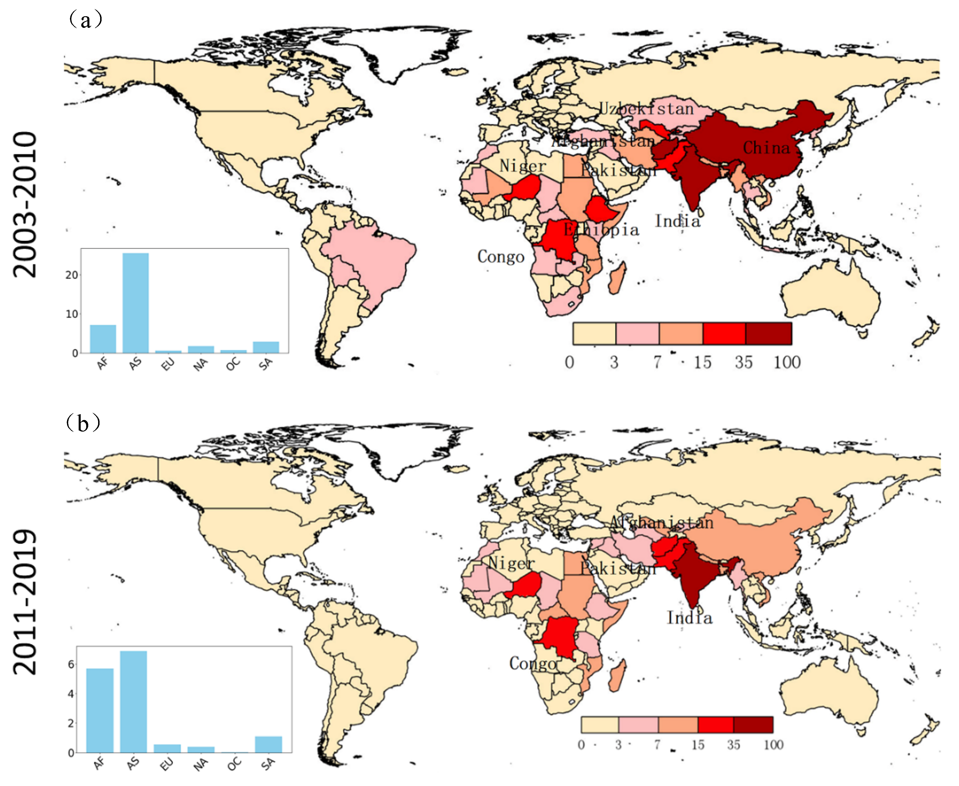
Water scarcity risk was evaluated using EHV framework and remote sensing. The proposed framework was applied to delineate global water stress levels for two distinct periods: 2003–2010 and 2011–2019. Water stress level was scaled to a range of 0–100 for ensuring consistency. Based on these scaled values, countries were further classified into five water stress risk categories, i.e., very high, high, medium, low, or very low, determined by the quantile-based thresholds.

In addition, emphasis was given to countries in the Global South, especially those in Asia and Africa, where water scarcity is compounded by socioeconomic inequalities. In these regions, we explored the relationships between water stress and socio-economic indicators, including GDP, population, agricultural water use, and non-agricultural water use.

3. Results

3.1. Accuracy of Reconstructed Dataset

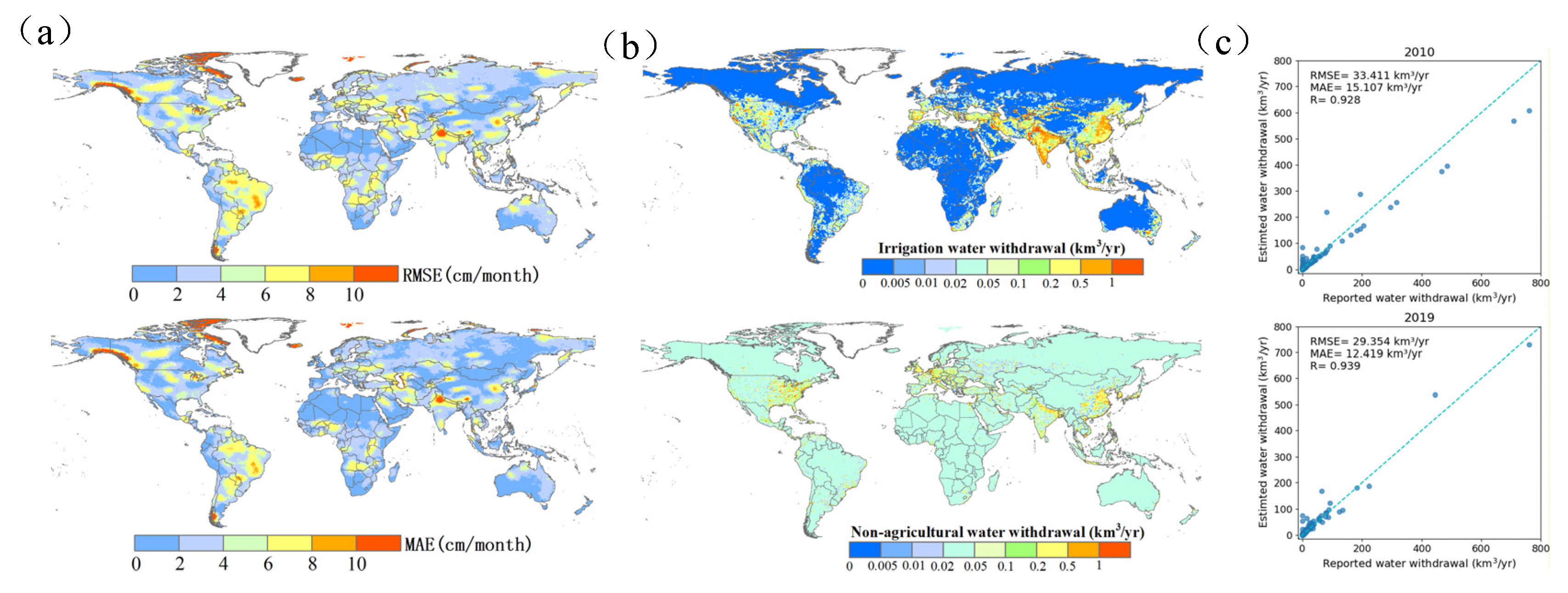
The reconstructed TWSA dataset was first validated using data from January 2006 to December 2019 as the training period to predict values for January 2003 to December 2005. Comparisons with GRACE-FO observations (Figure 2a) demonstrated a mean RMSE of 6.46 cm/month and a mean absolute error (MAE) of 5.83 cm/month. Spatial analyses revealed higher discrepancies in areas with intensive irrigation, groundwater extraction, and active glaciers, underscoring the influence of both human and natural factors. These results validate the reliability of the reconstructed dataset, making it a valuable tool for water resource assessments.

The calibrated water withdrawal dataset illustrates a refined representation of water withdrawals (Figure 2b), substantially improving the ability of WaterGAP in representing actual water use. Specifically, high-irrigation regions such as India, Pakistan, the North China Plain, and the United States showed improved alignment with observed data (Figure S4). To evaluate the performance of the emulator, the calibrated dataset was compared with reported values from the FAO AQUASTAT dataset, specifically focusing on total water withdrawal at the country level for the years 2010 and 2019 (Figure 2c). The emulator demonstrates high reliability at capturing water withdrawal patterns, suggesting that such a model enhances the precision of water resource analyses and provides a reliable foundation for further studies.

3.2. TWS Dynamic over Past Two Decades

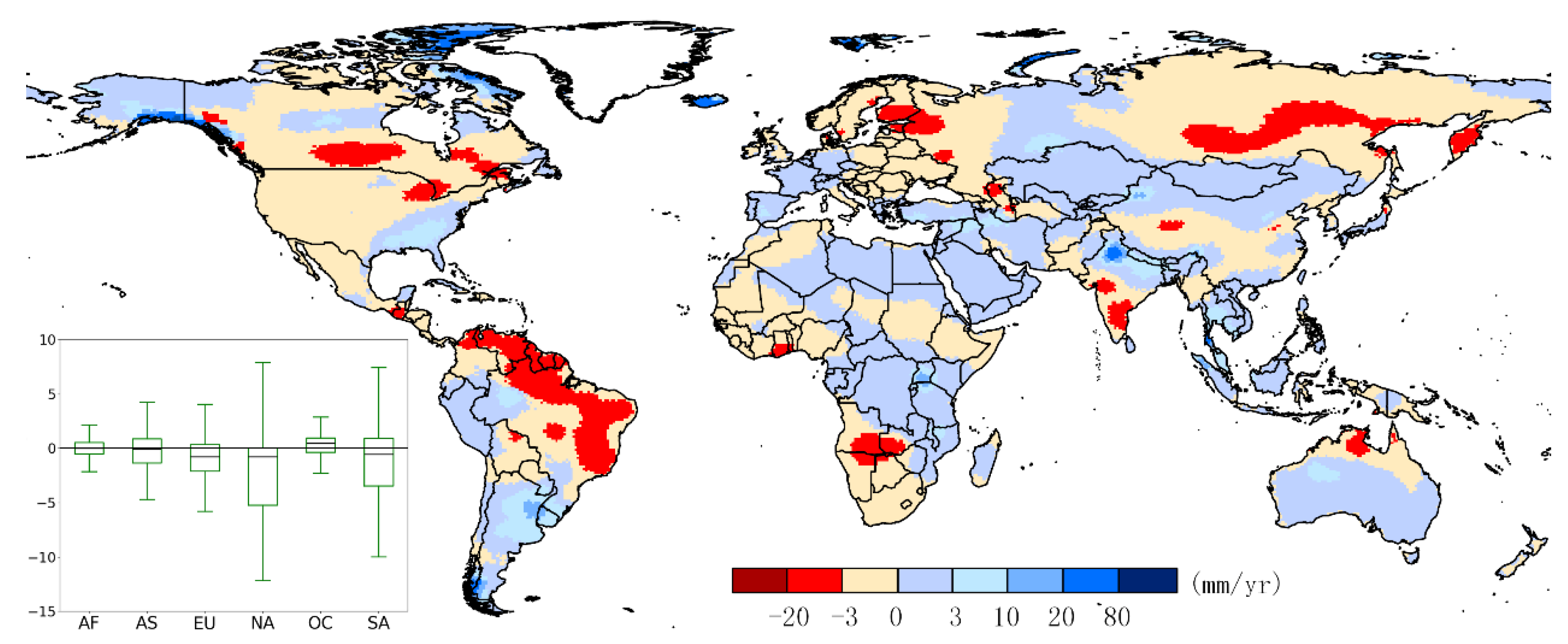
Satellite-derived observations combined with a data driven-reconstructed dataset reveal distinct spatial patterns of TWS across continents from 2003 to 2019. As shown in Figure 3, regions such as the Mongolian Plateau, Central Asia, Northern and Central Africa, and large parts of South America typically exhibit higher TWS, reflecting areas of sustained water availability. In contrast, Northeast Asia, Eastern Europe, Southern Africa, much of North America, and Northeastern South America show consistently lower TWS levels. The primary regions experiencing lower TWS are mainly distributed near latitudes 15° to 60°, including critical areas such as the Tibetan Plateau and the Amazon Basin, both of which serve as vital water sources for downstream transboundary rivers. North America emerges as the continent with the highest TWS variability reflecting fluctuations in water availability. Among other continents, the order of TWS variance from highest to lowest is South America, Europe, Asia, Oceania, and Africa. Notably, South America’s continent-wide median TWS remains relatively high, indicating strong storage capacity despite sub-regional heterogeneity.

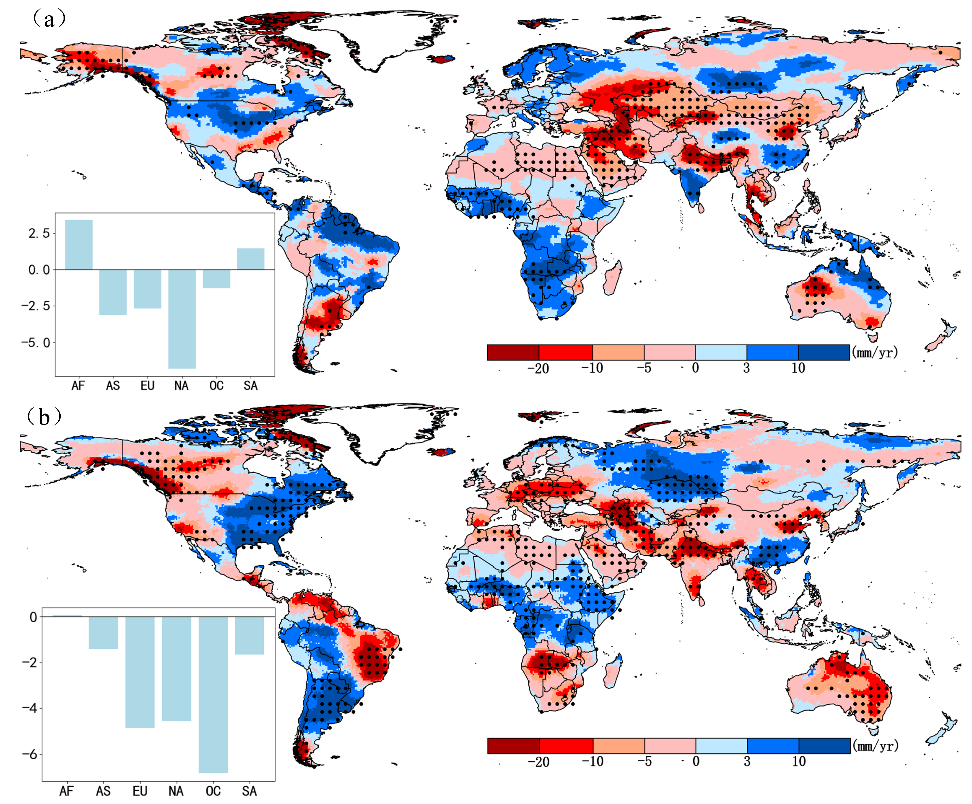
Figure 4 reveals a general TWS decline in several critical regions, including northern North America, the Siberian Plateau, and the Tibetan Plateau, with rates exceeding −10 mm/year. These trends can be attributed to the combined impacts of intensive irrigation practices, groundwater extraction, and glacial melt induced by global warming [46]. For example, the Tibetan Plateau, a vital “water tower” for much of Asia, has experienced accelerated ice loss, compounding the decline in TWS [47]. Similarly, the Siberian Plateau and northern North America are confronted with scarce water challenges driven by both cryosphere dynamics and anthropogenic water demands. Regions such as the Mongolian Plateau, areas surrounding the Mediterranean, and the eastern Amazon Plain also exhibit declining TWS trajectories. These patterns may be linked to large-scale land use changes, such as afforestation campaigns or anthropogenic destruction of rainforest environments, that have altered local hydrological cycles. Deforestation in the eastern Amazon has altered regional evapotranspiration patterns, leading to reduced soil moisture and diminished groundwater recharge. By contrast, much of South America maintains comparatively high storage and shows a smaller net decline than other continents. This is related to the fact that increases in the southern cone partly offset decreases in the eastern Amazon and Nordeste, yielding a modest continent-scale trend.

In addition, several regions, including Southeastern China, West Africa, Central and South America, and the northeastern United States, exhibit increasing TWS, with trends exceeding 7 mm/year. These gains are potentially linked to improved water resource management, reforestation initiatives, and increased precipitation due to regional climatic variability [45]. For example, southeastern China has benefited from large-scale ecological restoration projects such as the Grain for Green Program, which has enhanced soil moisture and water retention. Further analysis reveals that all continents experience a net decline in TWS except Africa and Oceania, and the decline in South America is comparatively small in the continental median. North America stands out with the most significant decrease, averaging −5 mm/year. This decline indicates the growing challenges of balancing water demands for agriculture and glacier melting, particularly in the context of a warming climate [48]. South America and Asia also exhibit substantial decreases, probably driven by deforestation in the Amazon Basin and intensive groundwater use in regions such as India, Pakistan and Central Asia, though the South American decline is spatially heterogeneous and damped by areas with persistent high storage.

3.3. Human Water Withdrawal over Past Two Decades

Using the global water withdrawal dataset reconstructed through remote sensing, geospatial data, and machine learning, we analyzed water withdrawal patterns and observed regional disparities closely linked to socio-economic development. As shown in Figure 5a, water withdrawal is relatively high in eastern and southeastern China, the Indian subcontinent, Southeast Asia, the northern Mediterranean coast, and parts of the United States and Mexico, with China having the highest water withdrawal. Additionally, some areas in Africa, such as parts of the Nile River Basin in Egypt and regions of South Africa, also exhibit extreme values of water withdrawal. In contrast, regions such as northern Asia, central Africa, Central and South America, northern North America, and western Australia show lower levels of water withdrawal. This distribution aligns closely with the global irrigation area percentage (Figure S1), highlighting the impact of agricultural irrigation on water demand.

At the continental level, Asia dominates global water withdrawal, exceeding 3500 km³/year, surpassing the withdrawal levels of other continents by $~$420%. In contrast, water withdrawal across other continents remains below 2000 km³/year, reflecting the vast population, extensive agricultural demands, and rapidly expanding industrial sectors in Asia. The top 20 regions with the highest water withdrawal are shown in Figure 5b. Specifically, China (1038 km³/year), the United States (743 km³/year), and India (688 km³/year) are the countries with the highest water withdrawal globally. The increased water demand in these regions is closely linked to their extensive irrigation needs, industrial development, and dense populations, driving water usage across agricultural, industrial, and domestic sectors. Despite the relatively high TWS levels in these countries, the distribution of water resources within their territories is highly uneven. Particularly, in China, India, and the United States, TWS is largely concentrated in glacier-fed and humid regions, which are often geographically distant from the primary centers of water demand. In contrast, the arid and semi-arid regions of these countries, such as northwestern India, northern China, and the southwestern United States, experience high agricultural water withdrawals but with severe water resource constraints, exacerbating regional imbalances in water availability.

3.4. Water Scarcity Assessment

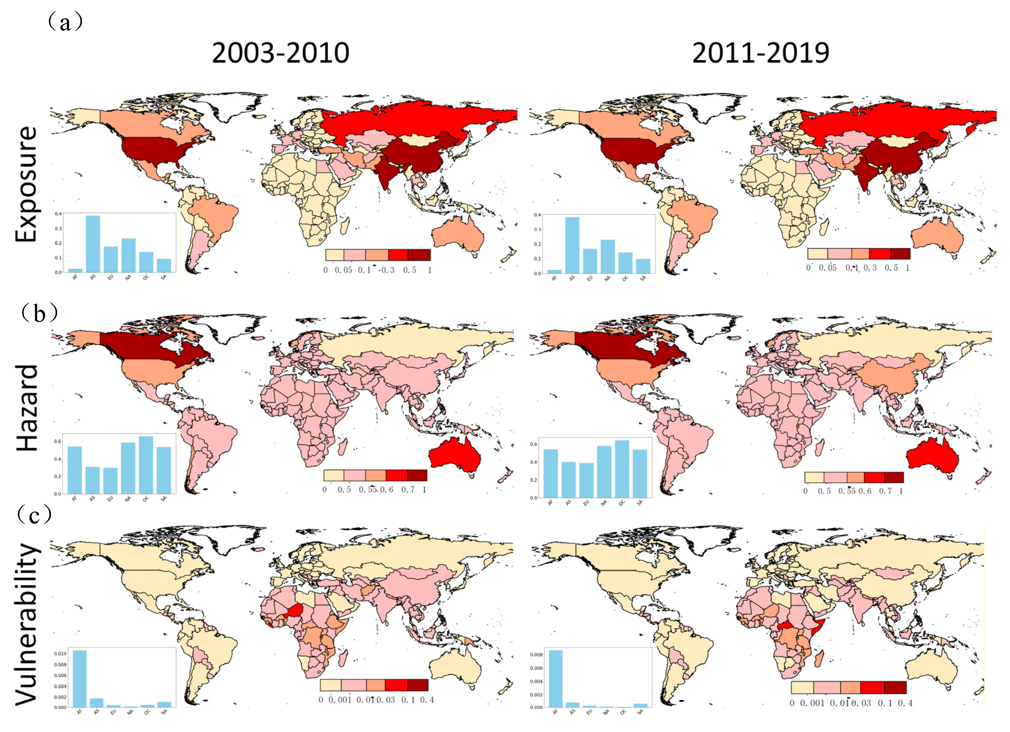
Global water scarcity was assessed using the exposure-hazard-vulnerability-framework, with a specific focus on its three components, i.e., exposure, hazard, and vulnerability. The spatial distribution of exposure (Figure 6a) remained largely consistent between 2003–2010 and 2011–2019. The highest exposure risks were concentrated in the United States and its surrounding regions, eastern and southern South America, eastern and central Asia, western Europe, and parts of Russia. In contrast, most of Africa, the Pacific Islands, and western South America exhibited lower exposure levels. Areas with higher exposure typically coincide with lower TWS, reflecting the impacts of intensive water withdrawals driven by industrial activities, high population density, and dependence on water-intensive sectors [49]. Conversely, low-exposure areas are generally associated with sparse populations and lower levels of industrialization [50,51]. Among the continents, Asia has the highest average exposure (approximately 0.5), followed by North America (approximately 0.3) and Europe (approximately 0.2).

The water-related hazard levels shown in Figure 6b reflect the combined impacts of drought conditions and governance inefficiencies. Overall, hazard levels have remained relatively stable across most regions, except for a slight increase observed in China. The highest hazard levels are concentrated in North America, Australia, and parts of Africa, including drought-prone areas such as the midwestern United States. In contrast, northern Europe and parts of South America exhibit lower hazard levels, likely due to fewer water-related threats and more effective governance systems. Although hazard levels are relatively uniform at the continental scale, specific regions such as Australia face substantial risks, primarily due to prolonged droughts driven by arid climatic conditions [52]. Continental assessments indicate that Africa, North America, Oceania, and South America have comparable hazard indices, with Oceania exceeding 0.6. In comparison, Asia and Europe display lower indices (around 0.3), which may reflect fewer drought-related disasters in Asia and Europe’s stronger governance capacity coupled with less frequent drought events.

The global distribution of the vulnerability index (Figure 6c) shows regional disparities in the capacity to cope with water emergencies. While most regions have maintained relatively constant levels of vulnerability, noticeable trends were observed in Africa and China. Vulnerability in China has decreased, likely associating with its substantial economic development and increased per capita GDP in recent years. Conversely, vulnerability in some regions of Africa has increased, particularly in Sub-Saharan Africa, East Africa, and parts of South Asia, probably driven by socioeconomic constraints such as poverty [53], political instability, and limited water resource management technologies. In contrast, North America and Europe have lower vulnerability levels, probably benefiting from higher HDI scores and adaptive capacities supported by ample economic resources. South America shows relatively low vulnerability on average. Higher continental TWS and strong socio-economic capacity help limit susceptibility to hydro-climatic stress, even where exposure exists.

The water stress index integrating exposure, hazard, and vulnerability (Figure 7) shows that high-risk areas are primarily concentrated in mid- to low-latitude regions. During 2003–2010, regions near the Tibetan Plateau, Central Asia, and large parts of Africa experienced elevated water stress. In the subsequent period (2011–2019), high-risk conditions persisted in the Tibetan Plateau and Central Asia, while central Africa saw a further expansion of dense high-risk zones. In most high-risk regions, there has been a reduction in risk levels over the two periods, particularly in Asia, where the average risk decreased by $~$73%. Southern Africa also experienced a notable decline in risk, likely linked to global economic development, especially the rapid economic growth in Asia over the past 20 years. Additionally, eastern and central Asia, along with northern, central, and eastern Africa, show higher water stress than other regions. In North America and China, exposure risk is high due to dense populations and industrial demand, but vulnerability is relatively low. This suggests that enhanced infrastructure and governance systems could mitigate these impacts. On the other hand, parts of Central Africa and South Asia have complex risks, where moderate hazard levels are exacerbated by high vulnerability. This combination makes these regions particularly susceptible to water crises, emphasizing the need for targeted interventions to enhance resilience in socioeconomically disadvantaged areas. By contrast, scarcity risk in South America remains comparatively low at the continental median, primarily because vulnerability is lower and storage buffers are stronger, which dampens the translation of exposure and hazard into high water-stress outcomes.

3.5. Evolution of Water Scarcity

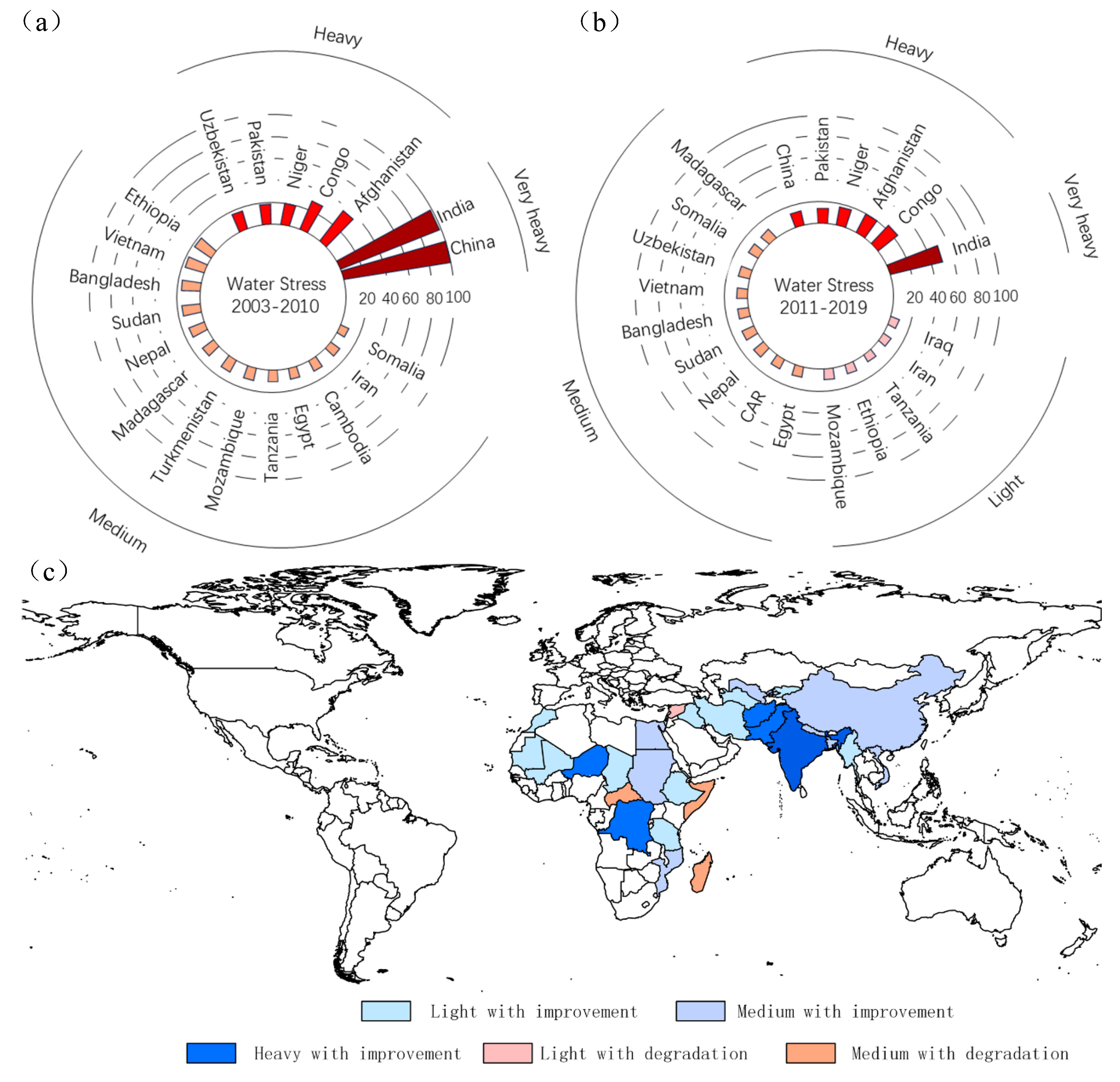
The evolution of water scarcity over the past two decades was further explored based on the developed water stress index. Figure 8a,b present the top 20 countries experiencing water scarcity and their associated risk levels. Between 2003 and 2010, China and India experienced particularly severe water stress. This was primarily driven by high agricultural and industrial demand, rapid population growth, which contributed to a sharp increase in water withdrawals and a subsequent reduction in TWS. At the same time, GE and HDI in these regions did not progress at a comparable rate, exacerbating their vulnerability. Similarly, countries such as Afghanistan, Congo, Nepal, Pakistan, and Uzbekistan experienced water stress due to regional drought, inefficient water resource management, and heavy reliance on agriculture. In Africa, nations such as Ethiopia, Sudan, Madagascar, and the Democratic Republic of Congo exhibited moderate to severe water stress, primarily due to the combined effects of climate change and weak water infrastructure [54]. The worsening water scarcity in these regions reflects declining levels of economic and social development, which increases their vulnerability to water crises.

Between 2011 and 2019, global water stress levels showed improvement. During this period, India became the region with the highest water stress globally, with a water stress index of 49. In contrast, China experienced an 85% reduction in its water stress, reflecting substantial progress in water resource management and infrastructure development. Despite these improvements, countries such as Congo, Afghanistan, Nepal, and Pakistan continued to undergo relatively high-water stress, indicating limited progress in water governance and sustained pressures from agricultural water demand. Meanwhile, countries like Somalia, Iraq, and Ethiopia experienced significant water stress due to a combination of human and environmental factors during this period, particularly political instability and the impact of climate change on water resource management.

The shifts in the global water stress index from the period 2003–2010 to 2011–2019 are illustrated in Figure 8c. Evolution in water stress indices in Asia and Africa over the past two decades, with an overall downward trend indicating substantial improvement, though some regions experienced slight increases. Pronounced declines were observed in southern Asia and central Africa. Although water stress levels have decreased in countries like China, India, and Sudan, these nations still experience substantial water constraints. Conversely, water stress levels have further increased in regions such as central Africa, Somalia, Madagascar, and Syria. This can be attributed to persistent droughts and political instability, which have led to an increase in the hazard index and a decline in GE and HDI. Frequent droughts and population growth have intensified water demand, while the lack of effective water management and infrastructure development has left these regions more vulnerable to water crises.

3.6. Socio-Economic Drivers of Water Scarcity

The relationship between socio-economic drivers and water scarcity was further analyzed, as displayed in Figure 9a. A weak negative correlation between GDP and water stress index is observed in African and Asian countries, particularly among smaller nations. Some countries possess abundant water resources yet display low levels of economic development, implying that wealthier nations are better positioned to alleviate water scarcity through financial and technological investments, such as implementing water reservoir and diversion projects, and adopting desalination techniques. Conversely, economically disadvantaged regions are often unable to deploy these resources, leaving them more vulnerable to severe water shortages despite their available natural resources. As depicted in Figure 9b, there is a stronger positive correlation between population and water stress index, particularly in Asia (r = 0.44). India and China stand out as prominent outliers, meaning that their large populations contribute to elevated water stress levels. In Africa, the correlation is somewhat weaker (r = 0.40), with countries like the Democratic Republic of Congo and Afghanistan emerging as notable examples. These findings highlight the compounding pressure of population growth on already limited water resources, especially in regions where infrastructure and management systems are underdeveloped.

Figure 9c illustrates a positive correlation between irrigation water use and water stress index in both Africa (r = 0.42) and Asia (r = 0.52), with the relationship being more pronounced in Asia. Countries such as China, Afghanistan, and the Democratic Republic of Congo demonstrate that intensive irrigation practices exacerbate water stress. This trend is particularly concerning in Asia, where the dependence on agricultural water use is more acute. In these regions, the imbalance between agricultural water demand and available resources perpetuates a cycle of resource depletion and increased stress on water systems. Similarly, a moderate positive correlation is observed between non-agricultural water use and water stress (Figure 9d), with Asia showing a slightly stronger relationship (r = 0.45) than Africa (r = 0.44). China and India again emerge as major outliers, suggesting that industrial and urban water demands are critical drivers of water stress in these regions. The overuse of water for non-agricultural purposes in economically developed areas often shifts the burden of scarcity to rural and underdeveloped regions. This means that the disparities in how water stress is managed globally. While Global South countries struggle with resource scarcity and uneven water distribution, wealthier regions such as North America, Western Europe, and even China are better equipped to mitigate water stress through advanced technologies and substantial infrastructure investments (Figure S5).

4. Discussion

4.1. Advancing Beyond Existing Approaches

This study proposes a novel framework for assessing global water scarcity by integrating the IPCC risk assessment paradigm with remote sensing, geospatial data, and machine learning. By reconstructing multi-year water storage and withdrawal dynamics over the past two decades, our approach bridges key data gaps and reduces the dependence of land surface hydrological models on uncertain meteorological inputs and parameterizations [55]. This reconstruction enhances the reliability of water resource assessments, particularly in data-scarce regions such as sub-Saharan Africa and the Middle East, where conventional monitoring networks are weak or absent. We also benchmarked three base learners against the BTCH ensemble and found that the ensemble consistently delivers lower RMSE/MAE and higher NSE than any single model (Figure S6a). In short, the base learners exhibit complementary tendencies, while the ensemble suppresses idiosyncratic errors and preserves shared signal, yielding more accurate and stable TWSA fields. Furthermore, these gains carry through when TWSA is propagated to vulnerability and risk, producing balanced smoother maps without overshoot (Figure S6b).

Traditional water scarcity assessments, typically based on withdrawal-to-availability ratios [56,57], fail to capture critical socio-economic dimensions, adaptive capacities, and dynamic responses to climate and policy shifts. Our framework addresses these gaps by incorporating multi-dimensional indicators that account for both natural variability and societal adaptation. It can identify the compounded impacts of extreme drought and population growth in high-stress regions such as South Asia and Africa. Existing frameworks such as the SDG Indicator 6.5.1 (Degree of Implementation of Integrated Water Resources Management, IWRM) and Water Footprint Assessment (WFA) provide valuable perspectives but remain limited. The IWRM index is largely static and omits integration of socio-environmental dynamics, while the WFA emphasizes efficiency over equity, neglecting water access disparities in vulnerable regions [58,59]. Regional assessments often lack scalability for global analysis, especially under transboundary governance and climate-induced water challenges. Our framework overcomes these constraints by integrating multi-source satellite observations and machine learning techniques to monitor dynamic changes in surface water, groundwater, glacier-fed flow, and reservoir storage [60,61]. This allows for a more spatially explicit representation of water resources, particularly in storage-dependent regions such as the North China Plain, Qinghai–Tibet Plateau, Andes, Rocky Mountains, and the upper Nile. Furthermore, the global consistency of datasets enables robust cross-regional comparisons and supports assessments of complex transboundary systems including the Mekong, Ganges, Indus, Colorado, and La Plata basins. We further compared our approach with several mainstream methods (

Table 2. Comprehensive comparative analysis of global water security assessment approaches.

ID	Approach	Study Region	Descriptions	Reference
1	Hydro-economic and water footprint diagnosis	Lake Urmia Basin, Iran	Establishing a direct link between agricultural water use (>85%) and ecological crises but remains static and omits adaptive capacity/governance.	Sobhani et al. [62]
2	Cross-system teleconnection analysis	Amazon-Pantanal Corridor, South America	Quantifying remote ecological dependence (>50% moisture contribution), but results are sensitive to moisture-tracking parameter choices.	Bergier et al. [63]
3	Groundwater depletion and drought response	Colorado River Basin, USA	Revealing >50% groundwater loss but focuses on a single component with limited surface-water integration.	Castle et al. [64]
4	Remote sensing technology monitoring	Global	Providing dynamic, meter-scale data in data-scarce regions, but indirect retrieval introduces ~10–30% uncertainty.	Chawla et al. [65]
5	Ecosystem services integrated modeling	Water-scarce areas (Regional scale)	Coupling ecosystem flows with water security, but high model complexity compounds uncertainty.	Qin et al. [66]
6	Atmospheric moisture tracking & source-sink analysis	Global	Quantifying transboundary moisture dependencies but is highly dependent on tracking algorithm assumptions.	Posada-Marín, Salazar, Rulli, Wang-Erlandsson and Jaramillo [11]
7	Integrating remote sensing, geospatial datasets, and ensemble machine learning techniques	Global	Reconstruct multi-year, high-resolution, globally consistent datasets; reduces reliance on parameterized land-surface models; integrates natural and socio-economic indicators.	This study

) and found comparable performance, while our method shows clear advantages and strong practical reference value.

Using TWS as the core factor for vulnerability is a principled choice within the EHV framework because it reflects buffer capacity rather than short-term variability. Compared with representing vulnerability by runoff or P-ET, TWS integrates surface, subsurface, and cryospheric storage into an observation-based indicator that is less sensitive to wet-dry regime shifts and less prone to double-count dryness signals already represented in Hazard (Figure S7). Moreover, TWS-driven vulnerability and the resulting risk are smoother and more stable, while preserving hotspot geography, especially in storage-dependent, groundwater-stressed regions, leading to more interpretable and policy-relevant country rankings.

4.2. Inequality and Implication in Water Resource Management

This study utilizes reliable multi-year datasets of water storage and withdrawal to investigate global water resource dynamics over the past two decades and their responses to climate change and socio-economic development. Our results reveal significant declines in water availability across several hotspots, particularly arid and semi-arid regions, while total withdrawals continue to rise. This divergence signals growing human-induced water stress, calling for urgent reassessment of current usage practices (Figure S8). Water stress is most acute in Asia and Africa, where climate variability is compounded by rapid agricultural expansion, industrial demands, and inadequate governance. These findings extend earlier work [67,68] by demonstrating the synergistic impacts of environmental and socio-economic drivers, underscoring the need for integrated assessment approaches.

The water scarcity index exhibits strong correlations with regional socio-economic disparities. In many Global South countries, economic growth often accelerates agricultural and industrial water demands, intensifying water stress, particularly in rural and low-income areas. Agriculture alone accounts for over 70% of total withdrawals in these regions yet offers relatively low economic returns and limited adaptive capacity. This highlights inefficiencies and equity challenges in water allocation and management. Further compounding the issue, many of the most water-stressed areas lie within transboundary river basins such as the Mekong, Indus, Nile, and Zambezi. In these basins, upstream nations often dominate water consumption, creating imbalances that disadvantage downstream communities [69,70]. By contrast, wealthier regions such as North America, Western Europe, and parts of East Asia exhibit greater resilience to water stress, supported by advanced technologies, infrastructure, and effective policy frameworks (Figures S5 and S8). These disparities highlight how economic capacity and institutional quality significantly influence water security outcomes. Collectively, our findings emphasize the urgent need for globally coordinated strategies to improve water efficiency, enhance governance, and promote equitable water distribution, particularly in vulnerable and transboundary regions.

4.3. Uncertainty Analysis and Limitations

Within the IPCC EHV framework, hazard denotes the propensity for adverse hydro-climatic stress under climate forcing. Accordingly, we construct with the self-calibrated PDSI (i.e., scPDSI), a physically based wet-dry indicator that aggregates water-balance anomalies with memory. To verify this, we benchmarked scPDSI against traditional PDSI and SPEI (standardized precipitation evapotranspiration index)-12 on a common dryness scale across two analysis windows (Figure S9a). scPDSI yields smoother arid-belt structure and less interannual choppiness in country aggregates while preserving the hotspot geography captured by SPEI. Country-level rank concordance remains high in the upper quintiles with minimal churn; where differences appear, they are concentrated in transitional climates where self-calibration is expected to add value. Dispersion metrics (i.e., rMAD and CV) for the hazard index across all countries and within the top 20% drought-prone group are moderate and closely aligned with SPEI-12, and lower than traditional PDSI in drylands, indicating reduced spurious volatility without damping genuine signals (Figure S9b). Taken together, scPDSI preserves the physical dryness patterns while improving tail stability and cross-climate comparability, supporting its use for global water-scarcity risk mapping in this study.

In interpreting cross-country differences, we use national totals only to convey the magnitude of potentially affected water-using systems, whereas vulnerability is where area/population-dependent intensity (i.e., per-area and per capita pressure) and capacity attributes (storage buffering, economic-technological buffers, and demand flexibility) are considered. Thus, a country with high total demand is not labeled “more exposed” by construction; instead, its manageability is reflected under vulnerability, while exposure remains a scale context. This E-V role separation avoids misleading comparisons driven by country size or population alone. Meanwhile, it should be mentioned that governance effectiveness can be placed in either hazard (as a moderator of dryness propensity) or vulnerability (adaptive capacity) in EHV studies. Here we adopt the former so that hazard reflects how institutional effectiveness conditions the translation of hydro-climatic dryness into hazardous stress, while vulnerability remains a strictly capacity-like construction (storage stocks and socio-economic development). Assigning GE to vulnerability is also defensible; yet it would mainly redistribute variance between hazard and vulnerability without altering the intended separation between variability and capacity or the qualitative risk patterns.

Despite above advantages, several shortcomings should be considered. First, the impacts of climate change on precipitation patterns and ET often exacerbate water shortages, especially those caused by extreme weather events. However, current methodologies may fall short in accurately capturing these complex variations. Additionally, water demand (driven by agricultural and industrial usage) varies seasonally and across watersheds, yet these patterns are often oversimplified or overlooked in existing assessment. Second, our framework primarily relies on country-level analyses, obscuring the specific hydrological dynamics of individual river basins. Refocusing assessments at the river basin scale would offer a more detailed and accurate representation of local water availability and demand. Third, although we mitigate observational gaps by reconstructing GRACE/GRACE-FO TWSA with an ensemble (and report uncertainty), TWS remains limited by coarse native resolution and sensor noise; withdrawal estimates also inherit uncertainties from remote-sensing proxies and sparse or inconsistent national reporting. Finally, the current framework treats all components, (i.e., exposure, hazard, and vulnerability) as equally weighted. This uniform weighting may not adequately reflect their varying in different regions. Assigning weights based on regional conditions, such as industrial or agricultural water demands, could improve the framework precision by better capturing the unique drivers of water stress in each area.

5. Conclusions

This study assesses two decades of global water dynamics and resulting water stress by reconstructing multi-year datasets from remote sensing, geospatial information, and ensemble machine learning. The reconstructed records reveal pronounced TWS declines in Northeast Asia, Northern Africa, and North America, where agricultural and industrial demand interact with climatic variability; withdrawals are highest in economically and agriculturally active regions, highlighting the difficulty of balancing use where consumption persistently outpaces natural replenishment. Within the EHV framework, we identify high exposure in densely populated areas (e.g., India and China), elevated hazard in drought-prone regions (e.g., North America and Australia), and marked vulnerability in parts of Africa and South Asia. Localized deteriorations in Central Africa, Somalia, Madagascar, and Syria likely reflect combined environmental and geopolitical pressures, whereas improvements in portions of China and India suggest that targeted interventions, such as infrastructure upgrades and water-saving policies, can measurably reduce stress. Correlations between water stress and GDP, population, and irrigation demand further illustrate how economic growth can intensify pressure and accentuate global inequalities.

The broader relevance of this work lies in providing storage- and withdrawal-aware evidence base for global comparison trend analysis and policy design. Concisely, the study contributes by: (i) delivering globally consistent multi-year reconstructions of TWS and withdrawals that reduce reliance on parameterized land-surface models; (ii) operationalizing a conceptually aligned risk framework in which hazard denotes dryness propensity and vulnerability denotes capacity, preserving the variability-capacity separation; and (iii) enabling robust cross-regional diagnostics and interpretable country rankings that highlight where storage deficits and human pressures most strongly elevate risk.

References

1. Wheeler, T.; von Braun, J. Climate Change Impacts on Global Food Security. Science 2013, 341, 508–513. [Google Scholar] [CrossRef] [PubMed]
2. Liu, K.; Li, X.; Wang, S.; Zhang, X. Unrevealing past and future vegetation restoration on the Loess Plateau and its impact on terrestrial water storage. J. Hydrol. 2023, 617, 129021. [Google Scholar] [CrossRef]
3. Li, X.; Mann, M.E.; Wehner, M.F.; Christiansen, S. Increased frequency of planetary wave resonance events over the past half-century. Proc. Natl. Acad. Sci. USA 2025, 122, e2504482122. [Google Scholar] [CrossRef] [PubMed]
4. Dai, A. Drought under global warming: A review. WIREs Clim. Chang. 2011, 2, 45–65. [Google Scholar] [CrossRef]
5. Peng, Y.; Zhang, H.; Zhang, Z.; Tang, B.; Shen, D.; Yin, G.; Li, Y.; Chen, X.; Hu, Z.; Habib Nazrollozoda, S. Future challenges of terrestrial water storage over the arid regions of Central Asia. Int. J. Appl. Earth Obs. Geoinf 2024, 132, 104026. [Google Scholar] [CrossRef]
6. Gosling, S.N.; Arnell, N.W. A global assessment of the impact of climate change on water scarcity. Clim. Chang. 2016, 134, 371–385. [Google Scholar] [CrossRef]
7. Liu, J.; Yang, H.; Gosling, S.N.; Kummu, M.; Flörke, M.; Pfister, S.; Hanasaki, N.; Wada, Y.; Zhang, X.; Zheng, C.; et al. Water scarcity assessments in the past, present, and future. Earth’s Future 2017, 5, 545–559. [Google Scholar] [CrossRef]
8. Zhang, Y.; He, B.; Guo, L.; Liu, J.; Xie, X. The relative contributions of precipitation, evapotranspiration, and runoff to terrestrial water storage changes across 168 river basins. J. Hydrol. 2019, 579, 124194. [Google Scholar] [CrossRef]
9. Hoff, H. Global water resources and their management. Curr. Opin. Environ. Sustain. 2009, 1, 141–147. [Google Scholar] [CrossRef]
10. Masih, I.; Uhlenbrook, S.; Maskey, S.; Ahmad, M.D. Regionalization of a conceptual rainfall–runoff model based on similarity of the flow duration curve: A case study from the semi-arid Karkheh basin, Iran. J. Hydrol. 2010, 391, 188–201. [Google Scholar] [CrossRef]
11. Posada-Marín, J.; Salazar, J.; Rulli, M.C.; Wang-Erlandsson, L.; Jaramillo, F. Upwind moisture supply increases risk to water security. Nat. Water 2024, 2, 875–888. [Google Scholar] [CrossRef]
12. Qin, Y.; Mueller, N.D.; Siebert, S.; Jackson, R.B.; AghaKouchak, A.; Zimmerman, J.B.; Tong, D.; Hong, C.; Davis, S.J. Flexibility and intensity of global water use. Nat. Sustain. 2019, 2, 515–523. [Google Scholar] [CrossRef]
13. Swami, D.; Parthasarathy, D. Dynamics of exposure, sensitivity, adaptive capacity and agricultural vulnerability at district scale for Maharashtra, India. Ecol. Indic. 2021, 121, 107206. [Google Scholar] [CrossRef]
14. Liu, Y.; Chen, J. Future global socioeconomic risk to droughts based on estimates of hazard, exposure, and vulnerability in a changing climate. Sci. Total Environ. 2021, 751, 142159. [Google Scholar] [CrossRef]
15. Zhang, Y.; Li, C.; Chiew, F.H.S.; Post, D.A.; Zhang, X.; Ma, N.; Tian, J.; Kong, D.; Leung, L.R.; Yu, Q.; et al. Southern Hemisphere dominates recent decline in global water availability. Science 2023, 382, 579–584. [Google Scholar] [CrossRef] [PubMed]
16. Lu, J.; Jia, L.; Menenti, M.; Zheng, C.; Hu, G.; Ji, D. The impacts of drought on water availability: Spatial and temporal analysis in the Belt and Road region (2001–2020). Int. J. Digit. Earth 2025, 18, 2449706. [Google Scholar] [CrossRef]
17. Cui, J.; Lian, X.; Huntingford, C.; Gimeno, L.; Wang, T.; Ding, J.; He, M.; Xu, H.; Chen, A.; Gentine, P.; et al. Global water availability boosted by vegetation-driven changes in atmospheric moisture transport. Nat. Geosci. 2022, 15, 982–988. [Google Scholar] [CrossRef]
18. Long, D.; Yang, W.; Scanlon, B.R.; Zhao, J.; Liu, D.; Burek, P.; Pan, Y.; You, L.; Wada, Y. South-to-North Water Diversion stabilizing Beijing’s groundwater levels. Nat. Commun. 2020, 11, 3665. [Google Scholar] [CrossRef]
19. Liu, K.; Li, X.; Long, X. Trends in groundwater changes driven by precipitation and anthropogenic activities on the southeast side of the Hu Line. Environ. Res. Lett. 2021, 16, 094032. [Google Scholar] [CrossRef]
20. Hugonnet, R.; McNabb, R.; Berthier, E.; Menounos, B.; Nuth, C.; Girod, L.; Farinotti, D.; Huss, M.; Dussaillant, I.; Brun, F.; et al. Accelerated global glacier mass loss in the early twenty-first century. Nature 2021, 592, 726–731. [Google Scholar] [CrossRef]
21. Yang, X.; You, W.; Tian, S.; Jiang, Z.; Wan, X. A Two-Step Linear Model to Fill the Data Gap Between GRACE and GRACE-FO Terrestrial Water Storage Anomalies. Water Resour. Res. 2023, 59, e2022WR034139. [Google Scholar] [CrossRef]
22. Wang, L.; Zhang, Y. Filling GRACE data gap using an innovative transformer-based deep learning approach. Remote Sens. Environ. 2024, 315, 114465. [Google Scholar] [CrossRef]
23. Duan, Y.; Bo, Y.; Yao, X.; Chen, G.; Liu, K.; Wang, S.; Yang, B.; Li, X. A Deep Learning Framework for Long-Term Soil Moisture-Based Drought Assessment Across the Major Basins in China. Remote Sens. 2025, 17, 1000. [Google Scholar] [CrossRef]
24. Bo, Y.; Li, X.; Liu, K.; Wang, S.; Li, D.; Xu, Y.; Wang, M. Hybrid Theory-Guided Data Driven Framework for Calculating Irrigation Water Use of Three Staple Cereal Crops in China. Water Resour. Res. 2024, 60, e2023WR035234. [Google Scholar] [CrossRef]
25. Liang, Y.; Ding, F.; Liu, L.; Yin, F.; Hao, M.; Kang, T.; Zhao, C.; Wang, Z.; Jiang, D. Monitoring water quality parameters in urban rivers using multi-source data and machine learning approach. J. Hydrol. 2025, 648, 132394. [Google Scholar] [CrossRef]
26. Li, H.; Liu, K.; Yang, B.; Wang, S.; Meng, Y.; Wang, D.; Liu, X.; Li, L.; Li, D.; Bo, Y.; et al. Continuous monitoring of grassland AGB during the growing season through integrated remote sensing: A hybrid inversion framework. Int. J. Digit. Earth 2024, 17, 2329817. [Google Scholar] [CrossRef]
27. Liu, K.; Li, X.; Wang, S.; Lu, S.; Bo, Y.; Zhou, G. Quantifying Past and Future Terrestrial Water Storage Scarcity Across China Through Midcentury. Earth’s Future 2025, 13, e2025EF006071. [Google Scholar] [CrossRef]
28. Liu, K.; Li, X.; Wang, S. Assessing reclamation potential of abandoned drylands using knowledge-guided machine learning (KGML) and remote sensing. Water Res. 2025, 288, 124623. [Google Scholar] [CrossRef]
29. Wada, Y.; Wisser, D.; Bierkens, M.F.P. Global modeling of withdrawal, allocation and consumptive use of surface water and groundwater resources. Earth Syst. Dynam. 2014, 5, 15–40. [Google Scholar] [CrossRef]
30. Save, H.; Bettadpur, S.; Tapley, B.D. High-resolution CSR GRACE RL05 mascons. J. Geophys. Res. Solid Earth 2016, 121, 7547–7569. [Google Scholar] [CrossRef]
31. Li, F.; Kusche, J.; Chao, N.; Wang, Z.; Löcher, A. Long-Term (1979-Present) Total Water Storage Anomalies Over the Global Land Derived by Reconstructing GRACE Data. Geophys. Res. Lett. 2021, 48, e2021GL093492. [Google Scholar] [CrossRef]
32. Sun, Z.; Long, D.; Yang, W.; Li, X.; Pan, Y. Reconstruction of GRACE Data on Changes in Total Water Storage Over the Global Land Surface and 60 Basins. Water Resour. Res. 2020, 56, e2019WR026250. [Google Scholar] [CrossRef]
33. Shao, X.; Zhang, Y.; Liu, C.; Chiew, F.H.S.; Tian, J.; Ma, N.; Zhang, X. Can Indirect Evaluation Methods and Their Fusion Products Reduce Uncertainty in Actual Evapotranspiration Estimates? Water Resour. Res. 2022, 58, e2021WR031069. [Google Scholar] [CrossRef]
34. Deng, S.; Liu, S.; Mo, X.; Jiang, L.; Bauer-Gottwein, P. Polar Drift in the 1990s Explained by Terrestrial Water Storage Changes. Geophys. Res. Lett. 2021, 48, e2020GL092114. [Google Scholar] [CrossRef]
35. Müller Schmied, H.; Cáceres, D.; Eisner, S.; Flörke, M.; Herbert, C.; Niemann, C.; Peiris, T.A.; Popat, E.; Portmann, F.T.; Reinecke, R.; et al. The global water resources and use model WaterGAP v2.2d: Model description and evaluation. Geosci. Model Dev. 2021, 14, 1037–1079. [Google Scholar] [CrossRef]
36. Siebert, S.; Döll, P.; Hoogeveen, J.; Faures, J.M.; Frenken, K.; Feick, S. Development and validation of the global map of irrigation areas. Hydrol. Earth Syst. Sci. 2005, 9, 535–547. [Google Scholar] [CrossRef]
37. Stuke, A.; Rinke, P.; Todorović, M. Efficient hyperparameter tuning for kernel ridge regression with Bayesian optimization. Mach. Learn. Sci. Technol. 2021, 2, 035022. [Google Scholar] [CrossRef]
38. Liu, K.; Li, X.; Wang, S.; Zhang, H. A robust gap-filling approach for European Space Agency Climate Change Initiative (ESA CCI) soil moisture integrating satellite observations, model-driven knowledge, and spatiotemporal machine learning. Hydrol. Earth Syst. Sci. 2023, 27, 577–598. [Google Scholar] [CrossRef]
39. van der Schrier, G.; Barichivich, J.; Briffa, K.R.; Jones, P.D. A scPDSI-based global data set of dry and wet spells for 1901–2009. J. Geophys. Res. Atmos. 2013, 118, 4025–4048. [Google Scholar] [CrossRef]
40. Kaufmann, D.; Kraay, A. Governance Indicators: Where Are We, Where Should We Be Going? World Bank Res. Obs. 2008, 23, 1–30. [Google Scholar] [CrossRef]
41. Turner, B.L.; Kasperson, R.E.; Matson, P.A.; McCarthy, J.J.; Corell, R.W.; Christensen, L.; Eckley, N.; Kasperson, J.X.; Luers, A.; Martello, M.L.; et al. A framework for vulnerability analysis in sustainability science. Proc. Natl. Acad. Sci. USA 2003, 100, 8074–8079. [Google Scholar] [CrossRef] [PubMed]
42. Trautmann, T.; Koirala, S.; Carvalhais, N.; Güntner, A.; Jung, M. The importance of vegetation in understanding terrestrial water storage variations. Hydrol. Earth Syst. Sci. 2022, 26, 1089–1109. [Google Scholar] [CrossRef]
43. Yin, J.; Slater, L.J.; Khouakhi, A.; Yu, L.; Liu, P.; Li, F.; Pokhrel, Y.; Gentine, P. GTWS-MLrec: Global terrestrial water storage reconstruction by machine learning from 1940 to present. Earth Syst. Sci. Data 2023, 15, 5597–5615. [Google Scholar] [CrossRef]
44. Kummu, M.; Taka, M.; Guillaume, J.H.A. Gridded global datasets for Gross Domestic Product and Human Development Index over 1990–2015. Sci. Data 2018, 5, 180004. [Google Scholar] [CrossRef] [PubMed]
45. Liu, K.; Li, X.; Wang, S.; Zhou, G. Past and future adverse response of terrestrial water storages to increased vegetation growth in drylands. npj Clim. Atmos. Sci. 2023, 6, 113. [Google Scholar] [CrossRef]
46. Long, D.; Pan, Y.; Zhou, J.; Chen, Y.; Hou, X.; Hong, Y.; Scanlon, B.R.; Longuevergne, L. Global analysis of spatiotemporal variability in merged total water storage changes using multiple GRACE products and global hydrological models. Remote Sens. Environ. 2017, 192, 198–216. [Google Scholar] [CrossRef]
47. Li, X.; Long, D.; Scanlon, B.R.; Mann, M.E.; Li, X.; Tian, F.; Sun, Z.; Wang, G. Climate change threatens terrestrial water storage over the Tibetan Plateau. Nat. Clim. Chang. 2022, 12, 801–807. [Google Scholar] [CrossRef]
48. Li, X.; Mann, M.E.; Wehner, M.F.; Rahmstorf, S.; Petri, S.; Christiansen, S.; Carrillo, J. Role of atmospheric resonance and land–atmosphere feedbacks as a precursor to the June 2021 Pacific Northwest Heat Dome event. Proc. Natl. Acad. Sci. USA 2024, 121, e2315330121. [Google Scholar] [CrossRef]
49. Pereira, L.S. Water, Agriculture and Food: Challenges and Issues. Water Resour. Manag. 2017, 31, 2985–2999. [Google Scholar] [CrossRef]
50. Huang, Z.; Hejazi, M.; Li, X.; Tang, Q.; Vernon, C.; Leng, G.; Liu, Y.; Döll, P.; Eisner, S.; Gerten, D.; et al. Reconstruction of global gridded monthly sectoral water withdrawals for 1971–2010 and analysis of their spatiotemporal patterns. Hydrol. Earth Syst. Sci. 2018, 22, 2117–2133. [Google Scholar] [CrossRef]
51. Yang, D.; Yang, Y.; Xia, J. Hydrological cycle and water resources in a changing world: A review. Geogr. Sustain. 2021, 2, 115–122. [Google Scholar] [CrossRef]
52. Falster, G.M.; Wright, N.M.; Abram, N.J.; Ukkola, A.M.; Henley, B.J. Potential for historically unprecedented Australian droughts from natural variability and climate change. Hydrol. Earth Syst. Sci. 2024, 28, 1383–1401. [Google Scholar] [CrossRef]
53. Nkiaka, E. Exploring the socioeconomic determinants of water security in developing regions. Water Policy 2022, 24, 608–625. [Google Scholar] [CrossRef]
54. Rodríguez, D.J.; Paltán, H.A.; García, L.E.; Ray, P.; George, S.F.S. Water-related infrastructure investments in a changing environment: A perspective from the World Bank. Water Policy 2021, 23, 31–53. [Google Scholar] [CrossRef]
55. Liang, Y.; Cao, C.; Zhu, X.; Gao, S.; Zhang, Y.; Ma, X. Unveiling hidden dynamics: Fine-scale mapping of groundwater-dependent ecosystems using multi-source Earth observations. Int. J. Digit. Earth 2025, 18, 2528636. [Google Scholar] [CrossRef]
56. Liu, X.; Liu, W.; Liu, L.; Tang, Q.; Liu, J.; Yang, H. Environmental flow requirements largely reshape global surface water scarcity assessment. Environ. Res. Lett. 2021, 16, 104029. [Google Scholar] [CrossRef]
57. Liu, W.; Liu, X.; Yang, H.; Ciais, P.; Wada, Y. Global Water Scarcity Assessment Incorporating Green Water in Crop Production. Water Resour. Res. 2022, 58, e2020WR028570. [Google Scholar] [CrossRef]
58. Harris, F.; Moss, C.; Joy, E.J.M.; Quinn, R.; Scheelbeek, P.F.D.; Dangour, A.D.; Green, R. The Water Footprint of Diets: A Global Systematic Review and Meta-analysis. Adv. Nutr. 2020, 11, 375–386. [Google Scholar] [CrossRef]
59. Hoekstra, A.Y.; Chapagain, A.K.; Van Oel, P.R. Advancing Water Footprint Assessment Research: Challenges in Monitoring Progress towards Sustainable Development Goal 6. Water 2017, 9, 438. [Google Scholar] [CrossRef]
60. Ahmed, M.; Sultan, M.; Wahr, J.; Yan, E. The use of GRACE data to monitor natural and anthropogenic induced variations in water availability across Africa. Earth Sci. Rev. 2014, 136, 289–300. [Google Scholar] [CrossRef]
61. Seyoum, W.M.; Milewski, A.M. Improved methods for estimating local terrestrial water dynamics from GRACE in the Northern High Plains. Adv. Water Resour. 2017, 110, 279–290. [Google Scholar] [CrossRef]
62. Sobhani, P.; Esmaeilzadeh, H.; Deljouei, A.; Wolf, I.D.; Marcu, M.V.; Sadeghi, S.M.M. Assessing water security and footprint in hypersaline Lake Urmia. Ecol. Indic. 2023, 155, 110955. [Google Scholar] [CrossRef]
63. Bergier, I.; Assine, M.L.; McGlue, M.M.; Alho, C.J.R.; Silva, A.; Guerreiro, R.L.; Carvalho, J.C. Amazon rainforest modulation of water security in the Pantanal wetland. Sci. Total Environ. 2018, 619, 1116–1125. [Google Scholar] [CrossRef] [PubMed]
64. Castle, S.L.; Thomas, B.F.; Reager, J.T.; Rodell, M.; Swenson, S.C.; Famiglietti, J.S. Groundwater depletion during drought threatens future water security of the Colorado River Basin. Geophys. Res. Lett. 2014, 41, 5904–5911. [Google Scholar] [CrossRef] [PubMed]
65. Chawla, I.; Karthikeyan, L.; Mishra, A.K. A review of remote sensing applications for water security: Quantity, quality, and extremes. J. Hydrol. 2020, 585, 124826. [Google Scholar] [CrossRef]
66. Qin, K.; Liu, J.; Yan, L.; Huang, H. Integrating ecosystem services flows into water security simulations in water scarce areas: Present and future. Sci. Total Environ. 2019, 670, 1037–1048. [Google Scholar] [CrossRef]
67. Alam, K. Farmers’ adaptation to water scarcity in drought-prone environments: A case study of Rajshahi District, Bangladesh. Agric. Water Manag. 2015, 148, 196–206. [Google Scholar] [CrossRef]
68. Mekonnen, M.M.; Hoekstra, A.Y. Four billion people facing severe water scarcity. Sci. Adv. 2016, 2, e1500323. [Google Scholar] [CrossRef]
69. Yuan, L.; Wu, X.; He, W.; Kong, Y.; Degefu, D.M.; Ramsey, T.S. Using the fuzzy evidential reasoning approach to assess and forecast the water conflict risk in transboundary Rivers: A case study of the Mekong river basin. J. Hydrol. 2023, 625, 130090. [Google Scholar] [CrossRef]
70. Lu, S.; Lian, Z.; Sun, H.; Wu, X.; Bai, X.; Wang, C. Simulating trans-boundary watershed water resources conflict. Resour. Policy 2021, 73, 102139. [Google Scholar] [CrossRef]
Figure 1. Flowchart of this study. (a) TWS reconstruction. (b) Water withdrawal calculation. (c) Overall flowchart involving data processing, model establishment and analysis.
Remotesensing 17 03999 g001
Figure 2. Evaluation reconstructed water storage and withdrawal dataset. (a) Accuracy of TWS anomalies, (b) Spatial distribution of irrigation water withdrawal and non-agricultural water withdrawal. (c) Accuracy of estimated total water withdrawal for 2010 and 2019, validated against reported water withdrawal data.
Remotesensing 17 03999 g002
Figure 3. Spatial patterns of TWS anomaly across the globe during 2003–2019. The boxplots in the bottom-left corner depict the average values by continent, where AF, AS, EU, NA, OC, and SA represent Africa, Asia, Europe, North America, Oceania, and South America, respectively. Black lines within the boxplots indicate median values, while the boxes and whiskers represent the interquartile range (25–75%) and the 5–95% percentiles, respectively, highlighting the variability of TWS across continents.
Remotesensing 17 03999 g003
Figure 4. Trends in TWS anomaly during the periods (a) 2003–2010, and (b) 2011–2019. The bar chart in the bottom-left corner presents the average trend values for each continent, with significant values at the 95% confidence level indicated by circle markers. Abbreviations: AF, Africa; AS, Asia; EU, Europe; NA, North America; OC, Oceania; SA, South America.
Remotesensing 17 03999 g004
Figure 5. Patterns of total water withdrawal. (a,b) Spatial distribution of total water withdrawal during 2003–2010 and 2011–2019, respectively, alongside the average values by continent. (c) Total water withdrawal for the top 20 countries, illustrating the magnitude and ranking of water use across nations during the study period.
Remotesensing 17 03999 g005
Figure 6. Spatial patterns of risk assessment components, (a) Exposure, (b) Hazard, and (c) Vulnerability, for the risk assessment framework during the periods 2003–2010 and 2011–2019, respectively. Abbreviations: AF, Africa; AS, Asia; EU, Europe; NA, North America; OC, Oceania; SA, South America.
Remotesensing 17 03999 g006
Figure 7. Water stress index derived from the risk assessment framework, for the period (a) 2003–2010, and (b) 2011–2019. Abbreviations: AF, Africa; AS, Asia; EU, Europe; NA, North America; OC, Oceania; SA, South America.
Remotesensing 17 03999 g007
Figure 8. Evolutions in water stress dynamics. Top 20 countries impacted by the water stress index during the period (a) 2003–2010, and (b) 2011–2019. (c) Shifts of the water stress index between these two periods.
Remotesensing 17 03999 g008
Figure 9. Influence of socio-economic variables on water stress across countries in Africa (AF) and Asia (AS). Correlation between the water stress index and four critical socio-economic factors: (a) GDP (with 95% confidence ellipses), (b) population, (c) agricultural water withdrawal, and (d) non-agricultural water withdrawal.
Remotesensing 17 03999 g009