Multiscale Attention-Enhanced Complex-Valued Graph U-Net for PolSAR Image Classification

Highlights

What are the main findings?

• A novel multiscale attention-enhanced complex-valued Graph U-Net (MAE-CV-GUNet) is proposed for PolSAR image classification.
• The designed multi-scale attention module (MSA) can achieve effective fusion of multi-scale features, and thereby achieve high-precision classification.

What is the implication of the main finding?

• The constructed complex-valued graph convolution network (CV-GCN) can effectively encode the amplitude and phase information of PolSAR, thereby making the model more discriminative and improving the classification accuracy.
• This work presents a multi-scale feature fusion mechanism based on MSA modules, which can accurately classify PolSAR images and is beneficial for the application of polarimetric remote sensing images.

Abstract

The powerful graph convolutional network (GCN) for polarimetric synthetic aperture radar (PolSAR) image classification generally relies on real-valued features, ignoring the phase information and thus limiting the modeling of complex-valued (CV) polarization characteristics. To address this issue, this paper proposes a novel multiscale attention-enhanced CV graph U-Net model, abbreviated as MAE-CV-GUNet, by embedding CV-GCN into a graph U-Net framework augmented with multiscale attention mechanisms. First, a CV-GCN is constructed based on the real-valued GCN, to effectively capture the intrinsic amplitude and phase information of the PolSAR data, along with the underlying correlations between them. This way can well lead to an improved feature representation for PolSAR images. Based on CV-GCN, a CV graph U-Net (CV-GUNet) architecture is constructed by integrating multiple CV-GCN components, aiming to extract multi-scale features and further enhance the ability to extract discriminative features in the complex domain. Then, a multiscale attention (MSA) mechanism is designed, enabling the proposed MAE-CV-GUNet to adaptively learn the importances of features at various scales, thereby dynamically fusing the multiscale information among them. The comparisons and ablation experiments on three PolSAR datasets show that MAE-CV-GUNet has excellent performance in PolSAR image classification.

1. Introduction

Polarimetric synthetic aperture radar (PolSAR) employs the transmission and reception of electromagnetic waves in multiple polarization states to acquire scattering information from surface targets. Owing to its insensitivity to weather, clouds, and illumination, PolSAR enables all-weather, all-day imaging, thereby drawing widespread interest in image interpretation research. The classification of PolSAR images is one of the research focuses in PolSAR image processing, which aims to assign each pixel to a predefined land cover category for efficient information extraction and scene interpretation. Its applications span various domains, including agricultural assessment [1], urban mapping [2], and targe detection [3], and beyond.

Traditional classification approaches mainly focus on feature extraction and the design of classifiers. Polarimetric target decomposition is a commonly used feature for PolSAR image classification. It can be broadly categorized into coherent decompositions methods and incoherent decompositions methods. Coherent decomposition expresses the scattering matrix as a sum of multiple scattering mechanisms derived from distinct basis scattering models [4,5,6]. Incoherent decomposition analyzes scattering characteristics through statistical methods including Freeman decomposition [7], Yamaguchi decomposition [8], and Cloude–Pottier decomposition [9]. In terms of classifier design, various machine learning methods have been developed based on different optimization objectives and constraints. These classifiers utilize extracted features to distinguish between data of different categories, thereby accomplishing the classification task. Representative methods include support vector machines (SVMs) [10], random forests (RFs) [11], and Markov random fields (MRFs) [12]. However, traditional feature extraction methods rely on manually designed models and algorithms, which are typically based on specific assumptions. As a result, they often struggle to capture the complex non-linear relationships within the data, limiting their generalization ability across different datasets.

Recently, deep learning has exhibited strong performance in PolSAR image classification due to its powerful feature representation capability [13,14]. Sparse autoencoders [15], deep belief networks [16], and convolutional neural networks (CNNs) [17] have been widely explored. In particular, CNNs are widely used for their ability to capture local structures and hierarchical features. Zhou et al. [18] first applied CNN to PolSAR image classification, achieving superior performance compared to traditional methods. Chen et al. [19] used polarimetric features as CNN input, achieving faster training and higher classification accuracy compared to coherence matrix-based CNNs. Hua et al. [20] integrated two CNN branches to extract polarimetric and spatial features, achieving good performance in small-sample PolSAR image classification. However, the above CNN-based classification methods use real-valued inputs, ignoring phase information and data integrity. In literature, the phase information can reveal the intrinsic scattering differences in image, addressing key ambiguities in PolSAR classification that amplitude alone cannot resolve [8,21]. To fully utilize the amplitude and phase information contained in the PolSAR complex-valued (CV) data, Zhang et al. [22] pioneered the CV-CNN method, thereby significantly improving classification accuracy over traditional real-valued networks. Building upon this foundation, Tan et al. [23] extended CV-CNN to 3D-CV-CNN, incorporating spatial-spectral feature learning while preserving complex relationships, thereby achieving further performance improvements. More recently, Alkhatib [24] successfully integrated CV-CNN with CV vision transformers, showing that holistic phase exploitation enables even more accurate PolSAR image interpretation. Hua et al. [13] introduced an adaptive gating mechanism into CV-CNN, enhancing the adaptability of model to CV scattering and improving classification accuracy. However, CNNs rely on fixed-size square convolution or pooling kernels, and have an implicit assumption of homogeneity within the kernel, neglecting actual boundary information. Moreover, its limited receptive field poses challenges in capturing long-range dependencies.

Graph convolutional networks (GCNs) [25] extend the traditional convolution to graph-structured data, featuring data-adaptive kernels and capturing long-range dependencies by aggregating information from neighboring nodes. Qin et al. [26] were the first to apply GCNs to exploit spectral and spatial information in hyperspectral images, significantly improving classification with limited labels. Mou et al. [27] developed a non-local graph-based GCN, enhancing the ability to model long-range dependencies between nodes. The challenge of using pixels as graph nodes lies in the high computational complexity. Sheng et al. [28] used superpixels as nodes and constructed a multi-scale GCN method, effectively reducing computational complexity and improving classification accuracy. Yang et al. [29] used pooling to build multiscale graphs, capturing boundary and spatial information. Gao et al. [30] proposed the Graph U-Net method, which introduces pooling and unpooling operations on graphs to implement graph downsampling and upsampling. This framework enables the network to systematically capture multi-scale information, providing a general approach for multi-scale graph representation learning. These developments collectively highlight multi-scale graph modeling as a vital approach for enhancing the ability of GNNs to comprehend complex spatial structures through systematic integration of local and global information.

In recent years, GCNs have been gradually explored for PolSAR image classification. However, research in this direction remains at a preliminary stage, with limited systematic methodologies and theoretical depth. Liu et al. [31] introduced multi-scale graph representations using Gaussian pyramid structures, providing new perspectives for modeling complex spatial relationships. Cheng et al. [32] developed a superpixel-level correction framework that effectively addressed scale sensitivity issues. Wang et al. [33] further proposed parallel multi-scale graph convolution and fusion strategies, expanding the approaches for multi-scale feature utilization. While previous work has validated the potential of GCNs for PolSAR classification, two critical limitations persist. (1) Most models operate in the real-number domain, discarding the complex-valued nature of PolSAR data and losing vital scattering mechanisms in phase information. (2) Multi-scale fusion typically uses fixed weights, lacking adaptive mechanisms to dynamically adjust scale importance based on content, which limits representation capacity in complex scenarios.

In the PolSAR image domain, existing multi-scale GCNs often use superpixels to construct graph nodes, preserving local homogeneity and object boundaries [34,35]. However, most methods rely on manually defined scales, and regions at different scales are independent of each other. This can cause boundary inconsistencies across scales, increasing the inaccuracy of boundary positions when fusing multi-scale features. To overcome this limitation, hierarchical superpixel segmentation organizes regions into multiple scales with natural inclusion relationships [36] and consistent boundaries. Moreover, this hierarchical organization inherently supports graph contraction and recovery. The resulting symmetric architecture ensures spatially aligned and semantically compatible features from different-scale GCNs, establishing a solid foundation for multi-level feature fusion.

Motivated by the above discussion, we propose a novel multiscale attention-enhanced CV graph U-Net model (MAE-CV-GUNet), for PolSAR image classification. The model extends GCN to the complex domain by constructing a CV-GCN for complex feature extraction. Then, a CV graph U-Net (CV-GUNet) is built to integrate multiple CV-GCNs with different graph structure for CV multi-scale feature extraction. Finally, we design a multiscale attention (MSA) mechanism for multi-scale feature enhancement. The main novelties and contributions of this paper are summarized as follows.

(1)

The constructed CV-GCN consists of a CV graph convolution (CV-GConv) layer, a CV batch normalization (CV-BN) layer, and a CV rectified linear unit (CReLU) layer. This construction can well promote effective capture of both amplitude and phase information to discriminate different land cover classes.

(2)

The proposed MAE-CV-GUNet constructs a hierarchical-aware structure (HiAS) based on the revised Wishart distance and color difference metric to enable full interaction multiscale superpixels, thereby realizing graph pooling and unpooling operations. On this basis, the CV-GUNet is designed by integrating multiple CV-GCN layers to further extract the multiscale features in PolSAR images.

(3)

Additionally, this paper introduces an MSA mechanism that dynamically learns the weights of features at different scales, enabling adaptive fusion of multiscale features and achieving accurate PolSAR image classification.

This paper is structured as follows: Section 2 provides a detailed introduction to the proposed MAE-CV-GUNet model. Section 3 details the comparative experimental results and analysis. Section 4 analyzes the performance of MAE-CV-GUNet through ablation studies, and Section 5 concludes this work.

2. Materials and Methods

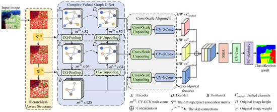
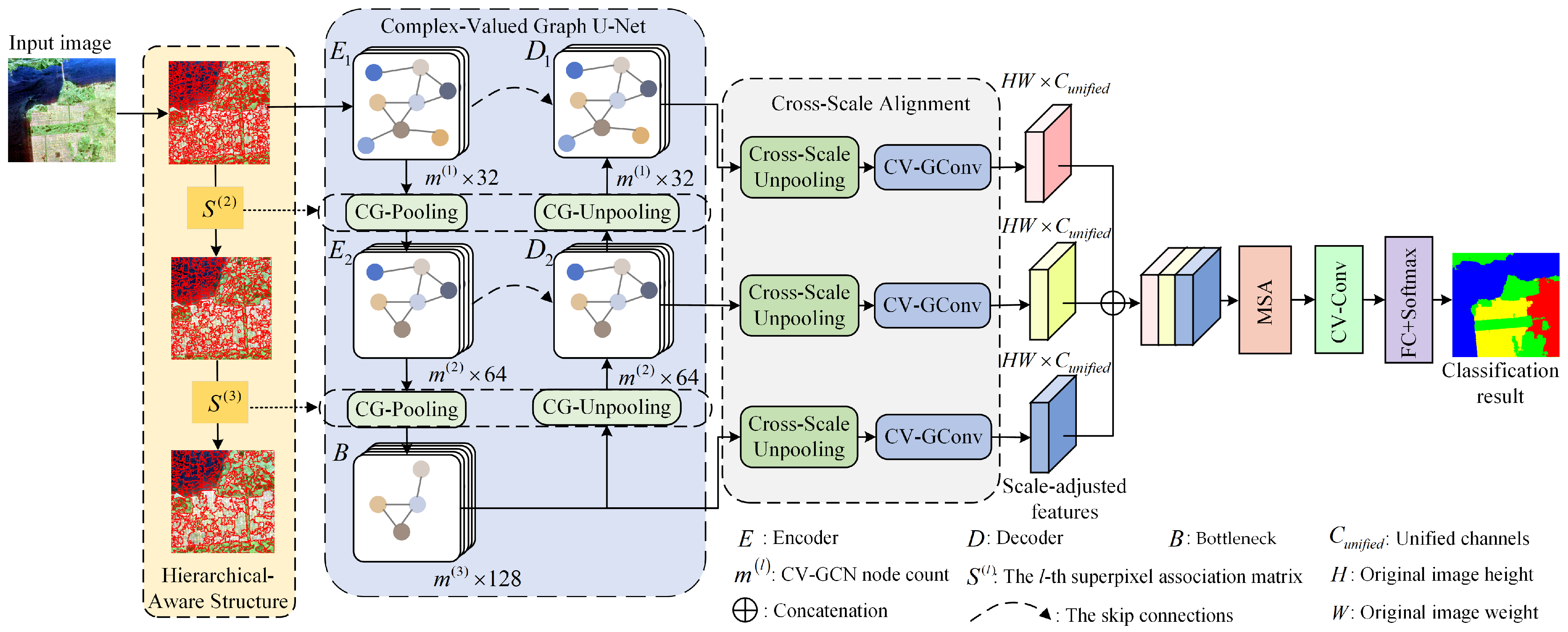
This section will detail the overall architecture of the MAE-CV-GUNet, which is illustrated in Figure 1. First, HiAS and its association matrices are obtained based on the input data. Second, CV-GUNet takes the first-layer superpixel features as input and uses the two association matrices for CV graph pooling (CG-Pooling) and CV graph upsampling (CG-Unpooling) to extract multiscale CV features. Subsequently, MSA realizes adaptive fusion and enhancement of the extracted multiscale features. Finally, the enhanced features are processed by a CV convolution layer (CV-Conv) which capture local features and further refine the features, followed by a fully connected layer and softmax for classification.

2.1. HiAS

The HiAS algorithm builds a hierarchically inclusive superpixel structure, allowing the Graph U-Net to effectively capture fine details and rich context across scales. In literature, manually designed multiscale strategies often suffer from cross-scale topological confusion in superpixel graphs of different scales. In this paper, we employ the hierarchical superpixel segmentation (HS) [36] to generate the HiAS of PolSAR images.

HS is a region merging method based on the minimum spanning tree (MST). For the undirected graph $\mathcal{G}=(\mathcal{V},\mathcal{E})$, HS initialize it as a forest with $\left|\mathcal{V}\right|$ subtrees. Here, $\mathcal{V}$ denotes the set of vertices, representing the sample points in the image, $\mathcal{E}$ denotes the set of edges, which reflect the connectivity or similarity between the sample points. Then, it utilizes the Boruvka algorithm [37], which is a bottom-up approach to identify the nearest neighbors connected by the least-weighted edge for each tree and merge them into a single cluster. This consolidation process is repeated until a forest is formed.

To adapt to the characteristics of PolSAR data, we use the revised Wishart distance [38] and color difference metric to construct edge weights. Specifically, the color distance is defined as the L1 distance between the Pauli decomposition components. The edge weights $D_{EW}$ can be computed as:

$$\begin{array}{cc}\hfill D_{RW}(i,j)& =\mathrm{tr}\left({\mathit{T}}_i^{-1}{\mathit{T}}_j\right)+\mathrm{tr}\left({\mathit{T}}_j^{-1}{\mathit{T}}_i\right)+ln|{\mathit{T}}_i|+ln|{\mathit{T}}_j|-q\hfill \\ \hfill D_{CD}(i,j)& ={∥\left(I_j\right)-\left(I_i\right)∥}_1\hfill \\ \hfill D_{EW}(i,j)& =\sqrt{D_{RW}^2(i,j)+\vartheta D_{CD}^2(i,j)}\hfill \end{array}$$

(1)

where $D_{RW}$ and $D_{CD}$ represent the revised Wishart distance and the color difference metric, respectively. ${\mathit{T}}_i$ denote the coherence matrices of the i-th trees, q represents the dimension of the coherence matrix, and $ln(·)$ and $tr(·)$ denote logarithmic and trace operations, respectively. $I_j$ denotes the Pauli components of the i-th samples, ${∥·∥}_1$ denotes the L1 distance, and $\vartheta$ is weighting parameter.

In practical applications, HS can flexibly generate multiple superpixel segmentations with arbitrary numbers of regions. Then, hierarchical-aware structure is generated, namely the HiAS. The HiAS maintains strict inclusion relationships across different hierarchical levels, where the structural correspondence between any two segmentation layers can be precisely characterized by an association matrix defined as:

$$S_{i,j}^{\left(l\right)}=\left\{\begin{array}{cc}1,\hfill & \mathrm{if}{C}_i^{(l-1)}\subseteq C_j^{\left(l\right)}\hfill \\ 0,\hfill & \mathrm{otherwise}\hfill \end{array}\right.$$

(2)

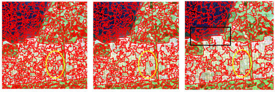
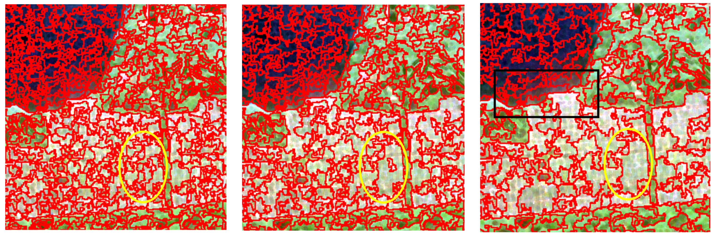
where $S^{\left(l\right)}\in {\mathbb{R}}^{m^{(l-1)}\times m^{\left(l\right)}}$ denotes the association matrix between the $(l-1)$-th and l-th layer superpixel segmentations, $m^{\left(l\right)}$ is the superpixel count in the l-th layer segmentations, and $l\in \{1,2,3\}$. $C_j^{\left(l\right)}$ is the j-th superpixel of the l-th layer segmentation, and $C^0$ denotes pixel of the input image. The HiAS is shown in Figure 2. The yellow circles highlight the inclusion relationships among the three segmentation maps, while the black boxes indicate the well-defined boundary segmentation.

2.2. CV-GUNet

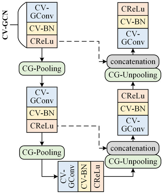
Graph U-Net [30] is an extension of the U-Net framework to graph-structured data, which employs GCNs to perform encoding and decoding on non-Euclidean data. Meanwhile, skip connections are used to concatenate features from the encoder and decoder, in order to mitigate the loss of shallow features. To better adapt to the characteristics of PolSAR data, we further modify the architecture into a CV-GUNet.

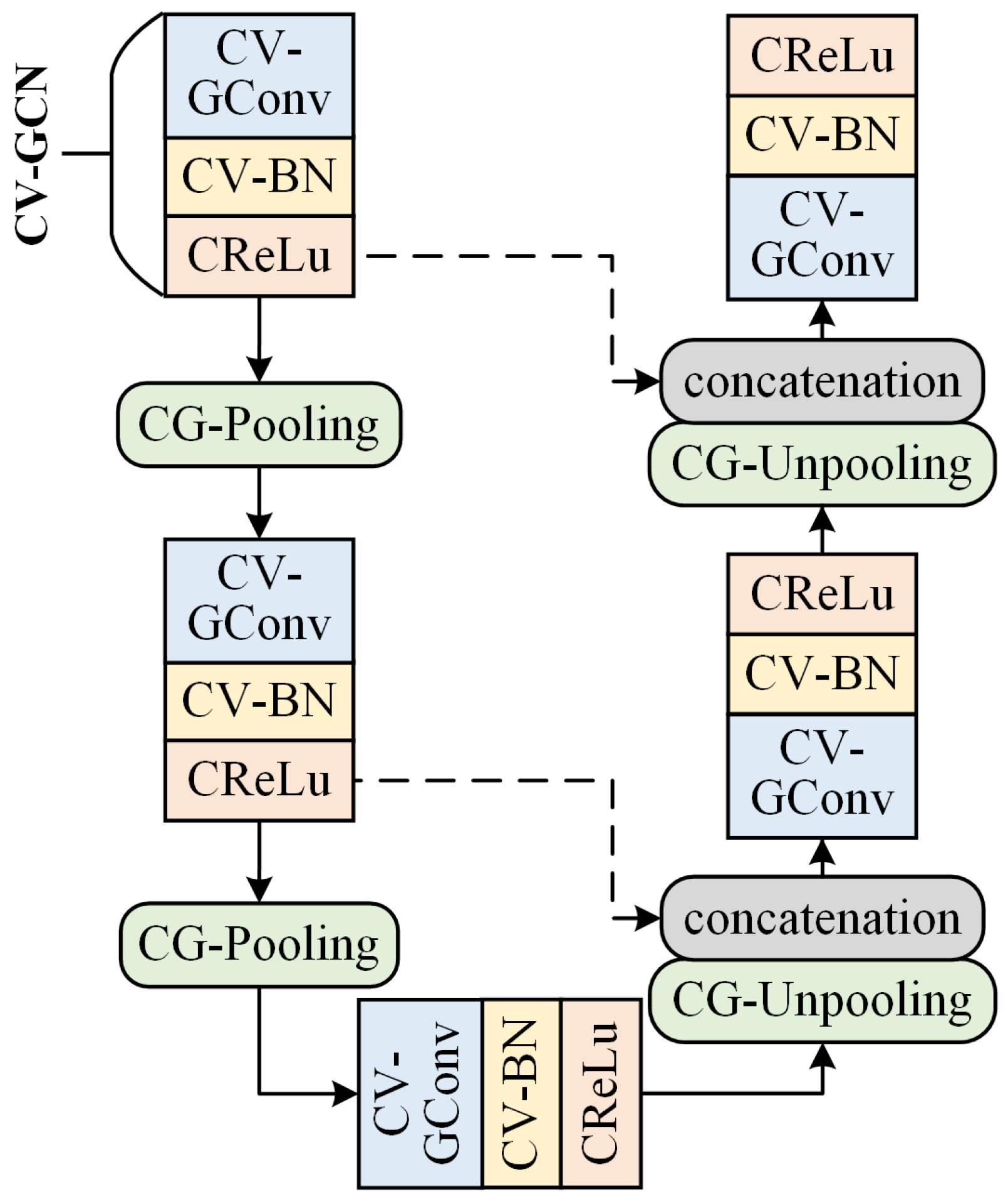
As shown in Figure 3, the encoders and decoders are built with CV-GCN and CV-GUNet comprises 2 encoders, 1 bottleneck, and 2 decoders. The black dashed lines indicate the skip connections between the encoders and the decoders. The core components of CV-GUNet, namely CV-GCN, CG-pooling and CG-unpooling, are described below.

2.2.1. Graph Construction

GCN models a PolSAR image as an undirected graph $\mathcal{G}=(\mathcal{V},\mathcal{E},\mathcal{A})$ to capture the relationships among sample points. Here, $\mathcal{A}\in {\mathbb{R}}^{\left|\mathcal{V}\right|\times \left|\mathcal{V}\right|}$ denote the pairwise connections between vertices. This ability to effectively learn from the data is fundamentally dependent on the graph structure. Consequently, the construction of the graph plays a crucial role in the feature extraction process of GCN. In CV-GUNet, the connection relationships among vertices are determined by the correlation of eight polarimetric features from the Yamaguchi and Cloude–Pottier decompositions as well as the Span, thereby yielding the initial association matrix ${\mathcal{A}}^0$:

$${\mathcal{A}}^0(i,j)=\left\{\begin{array}{cc}1,\hfill & \mathrm{if}{\overline{f}}_i\in \mathrm{KNN}\left({\overline{f}}_j\right)\hfill \\ 0,\hfill & \mathrm{otherwise}\hfill \end{array}\right.$$

(3)

where ${\overline{f}}_i$ denotes the average polarization feature within the superpixel $C_i$, and $\mathrm{KNN}(·)$ denotes the k-nearest neighbor operation. ${\mathcal{A}}^0(i,j)=1$ indicates that there is a connection between vertices i and j, while 0 denotes its absence.

To reduce the impact of inaccurate graph structures on subsequent classification tasks, this paper uses an attention mechanism to dynamically compute the node connection weights during training based on the output features H of the CV-GConv, enabling progressive refinement of the graph structure. The aforementioned adjacency matrix can be expressed as:

$$\mathcal{A}=\mathrm{softmax}\left(\mathrm{sigmoid}\left(\tilde{H}{\tilde{H}}^{\top }\right){\mathcal{A}}^0+\epsilon I\right)$$

(4)

where $\epsilon$ is a learnable parameter and ${(·)}^{\top }$ denotes the transpose operation. $\mathrm{sigmoid}(·)$ maps the input to a probability vector containing 0 and 1, and then $\mathrm{softmax}(·)$ normalizes it into a probability distribution. $\tilde{H}$ represents the output features of the GCN layer projected into a higher-dimensional space via a linear transformation, enhancing their representational capacity. $\tilde{H}$ can be expressed as:

$$\tilde{H}=(H_r{U}_r-H_i{U}_i)+i(H_r{U}_i+H_i{U}_r)$$

(5)

where $U_r$ and $U_i$ represent the real and imaginary parts of the weights in a CV linear layer, separately.

2.2.2. CV-GCN

Traditional GCNs extract features from graph-structured data by iteratively aggregating information from a node and its neighbors. This message-passing mechanism enables the model to capture spatial topology and learn discriminative, spatially correlated features. This process can be formally defined as follows:

$$\begin{array}{cc}\hfill H^{(l+1)}& =\sigma \left(\mathcal{A}{H}^{\left(l\right)}{W}^{\left(l\right)}\right)\hfill \end{array}$$

(6)

where $H^{\left(l\right)}$ and $H^{(l+1)}$ denote the value of the input and output for graph convolution layer (GConv), respectively. $\sigma$ denotes the activation function. $W^{\left(l\right)}$ is the trainable weight matrix at layer l. However, this forward propagation process focuses solely on aggregating neighbor information while ignoring the node itself. To address this, self-loops are added to the adjacency matrix, resulting in $\tilde{\mathcal{A}}=\mathcal{A}+I$, where I is the identity matrix.

In practice, $\tilde{\mathcal{A}}$ is typically symmetrically normalized to mitigate the influence of node degrees and improve numerical stability. The symmetrically normalized adjacency matrix $\widehat{\mathcal{A}}$ can be expressed as:

$$\widehat{\mathcal{A}}={\tilde{\mathbf{D}}}^{-{\displaystyle \frac{1}{2}}}\tilde{\mathcal{A}}{\tilde{\mathbf{D}}}^{-{\displaystyle \frac{1}{2}}}$$

(7)

where $\tilde{\mathbf{D}}$ denotes the degree matrix, a diagonal matrix derived from the adjacency matrix $\widehat{\mathcal{A}}$. Its diagonal elements, ${\tilde{\mathbf{D}}}_{ii}$, quantify the degree of each node i, which is the number of edges incident to it. Thus, the forward propagation of GConv can ultimately be expressed as

$$H^{(l+1)}=\sigma \left(\widehat{\mathcal{A}}{H}^{\left(l\right)}{W}^{\left(l\right)}\right)$$

(8)

The proposed CV-GCN consists of CV-GConv, CV-BN, and CReLU for processing CV graph data. In this paper, we construct the CV-GCN by introducing CV operations into GCN. Then, the forward propagation form of the $(l+1)$-th CV-GConv can be obtained as follows:

$$\begin{array}{cc}\hfill H^{(l+1)}& ={\sigma }_c(\mathbf{G}·\mathbf{W})\hfill \\ \hfill & ={\sigma }_c\left((\widehat{\mathcal{A}}{H}_r^{\left(l\right)}{W}_r^{\left(l\right)}-\widehat{\mathcal{A}}{H}_i^{\left(l\right)}{W}_i^{\left(l\right)})+i(\widehat{\mathcal{A}}{H}_i^{\left(l\right)}{W}_r^{\left(l\right)}+\widehat{\mathcal{A}}{H}_r^{\left(l\right)}{W}_i^{\left(l\right)})\right)\hfill \end{array}$$

(9)

where $\mathbf{G}$ represents the graph-structured features, $\mathbf{W}$ is the trainable weight matrix. $H_r^{\left(l\right)}$ and $H_i^{\left(l\right)}$ denote the real and imaginary parts of the output features from the l-th layer, respectively. ${\sigma }_c$ denotes the CV activation function CReLU.

The CV-BN is theoretically derived by analogy to the real-valued case, with the corresponding formulation shown below:

$$\begin{array}{c}BN\left(\tilde{o}\right)=\gamma ·\tilde{o}+\beta ,\tilde{o}={\left(V\right)}^{-{\displaystyle \frac{1}{2}}}(o-\mathbb{E}\left[o\right])\\ V=\left(\begin{array}{cc}{V}_{rr}& V_{ri}\\ V_{ri}& V_{ii}\end{array}\right)=\left(\begin{array}{cc}Cov\left(R\right(o),R(o\left)\right)& Cov\left(R\right(o),I(o\left)\right)\\ Cov\left(I\right(o),R(o\left)\right)& Cov\left(I\right(o),I(o\left)\right)\end{array}\right)\end{array}$$

(10)

where V is the covariance matrix in complex domain, $\mathbb{E}[·]$ denotes the mean operation applied separately to the real and imaginary parts, $Cov(·)$ denotes the covariance operation, and $R\left(o\right)$ and $I\left(o\right)$ denote the real and imaginary parts of feature o, respectively. $\gamma$ and $\beta$ are trainable parameters.

CReLU separately applys the ReLU activation function to the real and imaginary parts, which is defined as:

$$\mathrm{CReLU}\left(x\right)=\mathrm{ReLU}\left(R\right(x\left)\right)+i·\mathrm{ReLU}\left(I\right(x\left)\right)$$

(11)

where the ReLU function is expressed as $\mathrm{ReLU}\left(x\right)=max(x,0)$.

2.2.3. CG-Pooling and CG-Unpooling

In the original Graph U-Net [30], pooling selects top-k nodes based on feature scores, ignoring spatial structure and potentially losing local continuity. In this paper, we perform HiAS-based pooling and unpooling, merging and expanding regions to preserve spatial continuity, object boundaries, and multi-scale hierarchical information, making it particularly suitable for PolSAR images. The proposed CG-Pooling and CG-Unpooling are implemented based on the multiscale superpixels extracted from HiAS. CG-Pooling achieves downsampling of the graph structure by aggregating information from neighboring nodes with similar characteristics, thereby effectively extracting and exploring large-scale feature information. The CG-Pooling function can be defined as:

$$F_{\mathrm{CG}\text{-}\mathrm{Pool}}\left(H^{(l-1)}\right)={\left({\mathcal{S}}^{\left(l\right)}\right)}^{\mathrm{T}}\left(H_r^{(l-1)}+i·H_i^{(l-1)}\right)$$

(12)

Thus, the forward propagation of the encoder can be expressed as:

$$\begin{array}{cc}\hfill H^{(l+1)}=& {\sigma }_c((\widehat{\mathcal{A}}{F}_{\mathrm{CG}\text{-}\mathrm{Pool}}{(H^{\left(l\right)})}_r,W_r^{\left(l\right)})-\widehat{\mathcal{A}}{F}_{\mathrm{CG}\text{-}\mathrm{Pool}}{(H^{\left(l\right)})}_i,W_i^{\left(l\right)})\hfill \\ \hfill & +i·(\widehat{\mathcal{A}}{F}_{\mathrm{CG}\text{-}\mathrm{Pool}}{(H^{\left(l\right)})}_i,W_r^{\left(l\right)}+\widehat{\mathcal{A}}{F}_{\mathrm{CG}\text{-}\mathrm{Pool}}{(H^{\left(l\right)})}_r,W_i^{\left(l\right)}))\hfill \end{array}$$

(13)

CG-Unpooling can compensate for the information loss caused by CG-Pooling, ensuring that the final output maintains the same spatial dimensions as the input. The CG-Unpooling function can be defined as:

$${\mathbf{F}}_{\mathrm{CG}\text{-}\mathrm{Upool}}\left(H^{\left(l\right)}\right)={\mathcal{S}}^{\left(l\right)}\left(H_r^{\left(l\right)}+i·H_i^{\left(l\right)}\right)$$

(14)

Therefore, the forward propagation of the decoder can be expressed as:

$$\begin{array}{cc}\hfill H^{(l+1)}=& {\sigma }_c(\left(\widehat{\mathcal{A}}{F}_{\mathrm{CG}\text{-}\mathrm{Unpool}}{\left(H^{\left(l\right)}\right)}_r,W_r^{\left(l\right)}\right)-\widehat{\mathcal{A}}{F}_{\mathrm{CG}\text{-}\mathrm{Unpool}}{\left(H^{\left(l\right)}\right)}_i,W_i^{\left(l\right)}\hfill \\ \hfill & +i·\left(\widehat{\mathcal{A}}{F}_{\mathrm{CG}\text{-}\mathrm{Unpool}}{\left(H^{\left(l\right)}\right)}_i,W_r^{\left(l\right)}+\widehat{\mathcal{A}}{F}_{\mathrm{CG}\text{-}\mathrm{Unpool}}{\left(H^{\left(l\right)}\right)}_r,W_i^{\left(l\right)}\right))\hfill \end{array}$$

(15)

2.3. Multiscale Attention Mechanism

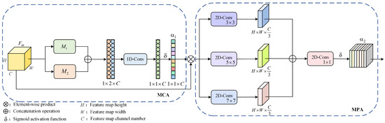
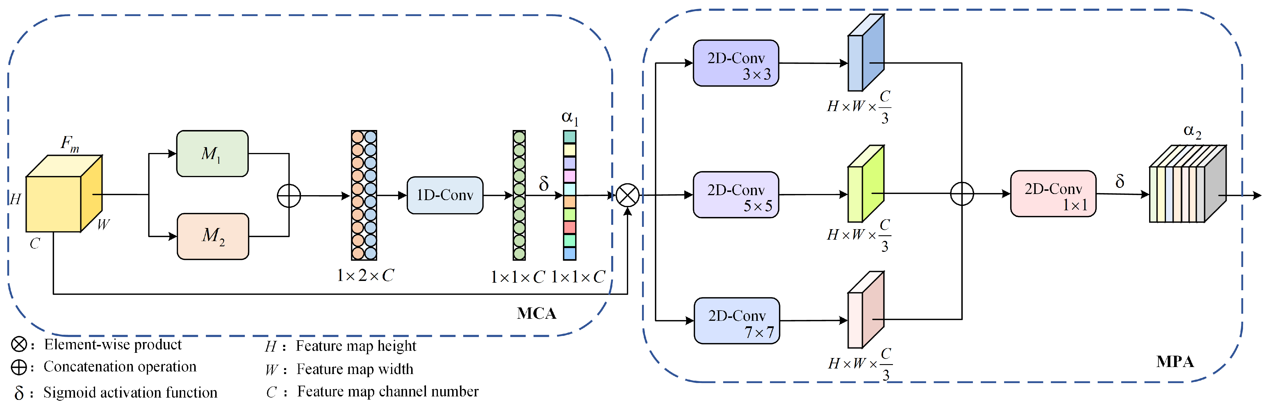
CV-GUNet equally treats all scale features, making it difficult to adapt to the multiscale characteristics of different ground object. To dynamically optimize the contribution of multiscale features, we propose the multiscale attention (MSA) mechanism, as illustrated in Figure 4. MSA module achieves effective feature fusion through progressive channel-to-spatial refinement. It first applies moment-based channel attention (MCA) to multiscale features to compute the importance weight ${\alpha }_1$. This weight modulates features and guides a multiscale spatial attention (MPA) module to focus on salient regions. The final output is a refined attention coefficient ${\alpha }_2$ that integrates both channel and spatial context.

2.3.1. Cross-Scale Alignment

To prepare the decoded multiscale features for subsequent fusion, we first aligned them to a consistent spatial size through cross-scale alignment. The decoded features at different scales are mapped to the original image size through the hierarchical relationships of HiAS. The cross-scale unpooling for the features $H_{D_1}$, $H_{D_2}$ and $H_b$ from decoder 1, decoder 2, and bottleneck is as follows:

$$\begin{array}{cc}\hfill H_{D_1}^{\downarrow }& =S^{\left(1\right)}{H}_{D_1}\hfill \\ \hfill H_{D_2}^{\downarrow }& =S^{\left(1\right)}{S}^{\left(2\right)}{H}_{D_2}\hfill \\ \hfill H_b^{\downarrow }& =S^{\left(1\right)}{S}^{\left(2\right)}{S}^{\left(3\right)}{H}_b\hfill \end{array}$$

(16)

where $H_{D_1}^{\downarrow }$, $H_{D_2}^{\downarrow }$ and $H_b^{\downarrow }$ represent the features $H_{D_1}$, $H_{D_2}$ and $H_b$ after scale adjustment, respectively. To reduce computational complexity, these features are projected through CV-GConv to obtain the unified 32-dimensional representation. Then, we concatenate the features from different scales into the multiscale feature $F_m$.

2.3.2. MSA Module

The global pooling in conventional channel attention mechanisms captures only first-order statistics of feature maps, limiting its expressive power. Inspired by [39], we replace it with high-order moment aggregation to construct a MCA module that captures richer distribution characteristics. Moments can reflect the statistical characteristics and distribution features of data, enabling the model to achieve better discriminative capability and a richer understanding of contextual information. Formally, let Y be bounded random samples from a distribution p. The generalized moment is defined as:

$$EM{A}_l\left(p\right)={\tau }_1{∥\mathbb{E}\left[Y\right]∥}_2+\sum _{l=2}^L{\tau }_l{∥M_l\left(Y\right)∥}_2$$

(17)

where $\mathbb{E}\left[Y\right]$ denotes the expectation of Y, ${\tau }_l$ represents the weighting parameters of each moment. $M_l\left(Y\right)$ represents the l-th order moment of Y, and $M_l\left(Y\right)=\mathbb{E}\left[{(Y-\mathbb{E}\left(Y\right))}^l\right]$. ${∥·∥}_2$ denotes the L2 norm operation.

This paper employs the first-order moment (mean) and the second-order moment (variance) for moment aggregation, which provides a good balance between simplicity and representational capacity. The mean and variance features are first extracted at each scale, then concatenated and fused through a 1D $3\times 3$ convolution, which guide the weighted integration of different moment features. A sigmoid function is subsequently applied to generate the corresponding weight coefficients ${\alpha }_1$. The process can be represented as:

$${\alpha }_1=\delta \left({\mathrm{Conv}}_{1\mathrm{D}}(M_1\left(F_m\right)\parallel M_2\left(F_m\right))\right)$$

(18)

where ‖ denotes the concatenation operation. $\delta$ denotes the sigmoid activation function. Thus, the features weighted by ${\alpha }_1$ can be represented as $F_1=F_m·{\alpha }_1$.

To achieve soft weight assignment for each pixel, enabling the allocation of different weights, the features $F_1$ are fed into MPA block to obtain the spatial attention coefficients ${\alpha }_1$. To enhance the ability of spatial attention to perceive structures at different scales, we employ multiscale 2D convolutional kernels in a parallel manner to extract contextual information and generate more accurate spatial attention weights in MPA. Specifically, convolutional kernels of sizes $3\times 3$, $5\times 5$, and $7\times 7$ are employed to encode multiscale spatial contextual relationships. Each convolution has one-third as many output channels as input channels. Then, the outputs of three branches are concatenated and fused through a $1\times 1$ convolution, producing the final multiscale attention coefficients ${\alpha }_2$:

$${\alpha }_2=\delta \left({\mathrm{Conv}}_{2\mathrm{D}}^{1\times 1}\left({\mathrm{Conv}}_{2\mathrm{D}}^{3\times 3}\left(F_1\right)\right)\parallel {\mathrm{Conv}}_{2\mathrm{D}}^{5\times 5}\left(F_1\right)\parallel {\mathrm{Conv}}_{2\mathrm{D}}^{7\times 7}\left(F_1\right)\right)$$

(19)

Notably, the attention aims to measure the importance contribution of features at different scales. To simplify the computation, the attention coefficients are calculated based on the magnitude of the complex features and directly applied to the real and imaginary parts of the features, thereby achieving weighted adjustment of the complex features.

2.4. Classification Module

A CV-Conv is applied to the enhanced features for fine-grained local processing. This single layer performs a lightweight integration and smoothing of the features, which produces a more robust and enriched representation without introducing unnecessary complexity. The CV features are then split into real and imaginary parts, passed through a fully connected layer and softmax layer for prediction. The softmax function is defined as:

$${\widehat{y}}_i={\displaystyle \frac{e^{z_i}}{{\sum }_{j=1}^Q{e}^{z_j}}},i=1,\dots ,Q$$

(20)

where $z_i$ denotes the score of category i, ${\widehat{y}}_i$ is the predicted the probabilities of class i, and Q denotes the total number of classes. Then, a class-weighted cross-entropy loss is used to train the network, measuring the prediction discrepancy and penalizing minority class errors with larger weights to combat imbalance. It is defined as:

$$\mathcal{L}=-{\displaystyle \frac{1}{N}}\sum _{n=1}^N\sum _{q=1}^Q{w}_q{y}_q^{\left(n\right)}log\left({\widehat{y}}_q^{\left(n\right)}\right)$$

(21)

where N denotes the number of samples, $w_q$ is the weight of class q, computed as the reciprocal of the number of samples in that class. $y_q^{\left(n\right)}=1$ indicates that the n-th sample belongs to class q, with all other classes set to 0.

2.5. PolSAR Data Processing

The scattering characteristics of a ground object can be represented by a $2\times 2$ complex scattering matrix $\mathit{S}$ as defined below

$$\mathit{S}=\left[\begin{array}{cc}{S}_{HH}& S_{HV}\\ S_{VH}& S_{VV}\end{array}\right]$$

(22)

where H denotes horizontal polarization and V denotes vertical polarization. ${\mathit{S}}_{HH}$ denotes the horizontally emitted, horizontally received backscattering coefficient.In the case of the Pauli basis under the single station reciprocity, the target vector $\mathit{k}$ of the polarization scattering matrix is expressed as follows

$$\mathit{k}={\displaystyle \frac{1}{\sqrt{2}}}\left[\begin{array}{c}{S}_{HH}+S_{VV}\\ S_{HH}-S_{VV}\\ 2S_{HV}\end{array}\right]$$

(23)

To avoid the randomness of scattering features, PolSAR data are often represented using second-order statistics. The coherence matrix is the most common representation of PolSAR data, and can be expressed as follows

$$T={\displaystyle \frac{1}{n}}\sum _{i=1}^n{\mathit{k}}_i{\mathit{k}}_i^{\mathrm{H}}=\left[\begin{array}{ccc}{T}_{11}& T_{12}& T_{13}\\ T_{21}& T_{22}& T_{23}\\ T_{31}& T_{32}& T_{33}\end{array}\right]$$

(24)

The superscript $\mathrm{H}$ indicates the conjugate transpose operation. As a Hermitian matrix satisfying $T_{ij}={\overline{T}}_{ji}$, T has six independent upper-triangular elements. They are selected as the initial input features for the HiAS architecture, thereby providing superpixel-level CV polarimetric information to enable subsequent model analysis and processing.

3. Experimental Results and Comparative Analysis

3.1. Experimental Setting

Table 1. Architectural configuration of MAE-CV-GUNet.

Module	Layer	Kernel Size@Number
CV-GUNet	Encoder1	@32
	Encoder2	@64
	Bottleneck	@128
	Decoder2	@64
	Decoder1	@32
Cross-Scale Alignment	CV-GConv	@32
CV-Conv	CV-Conv	$5\times 5$ @96
MSA	1D-Conv	3 @1
	2D-Conv (scale1)	$3\times 3$ @32
	2D-Conv (scale2)	$5\times 5$ @32
	2D-Conv (scale3)	$7\times 7$ @32
	2D-Conv (after concatenation)	$1\times 1$ @96

summarizes the architectural configuration of the MAE-CV-GUNet network. The model was trained using an initial learning rate of 0.005, a maximum of 300 epochs, and the Adam optimizer. Our approach utilized a 3-layer HiAS for large-scale PolSAR images, complemented by a fixed weighting parameter $\vartheta$ of 0.8. The dataset-specific configurations of the HiAS are detailed in

Table 2. HIAS SETTING FOR EACH DATASET.

Dataset	Superpixel Count per Layer
	Layer1	Layer2	Layer3
San Francisco	8000	4000	2000
Flevoland	6000	3000	1500
Oberpfaffenhofen	6000	3000	1500

. For the San Francisco, Oberpfaffenhofen, and Flevoland datasets, 2%, 5% and 2% of the labeled samples were randomly selected for training, respectively. All experimental results represent averages from ten runs, with all experiments conducted on a desktop computer (Windows 10, 11th Gen Intel i9-11900F CPU, NVIDIA GeForce RTX 3090 GPU) using PyTorch (version 1.11.0).

3.2. Experimental Data and Evaluation Metrics

The effectiveness of the proposed MAE-CV-GUNet is validated on three widely-used measured PolSAR image classification datasets:

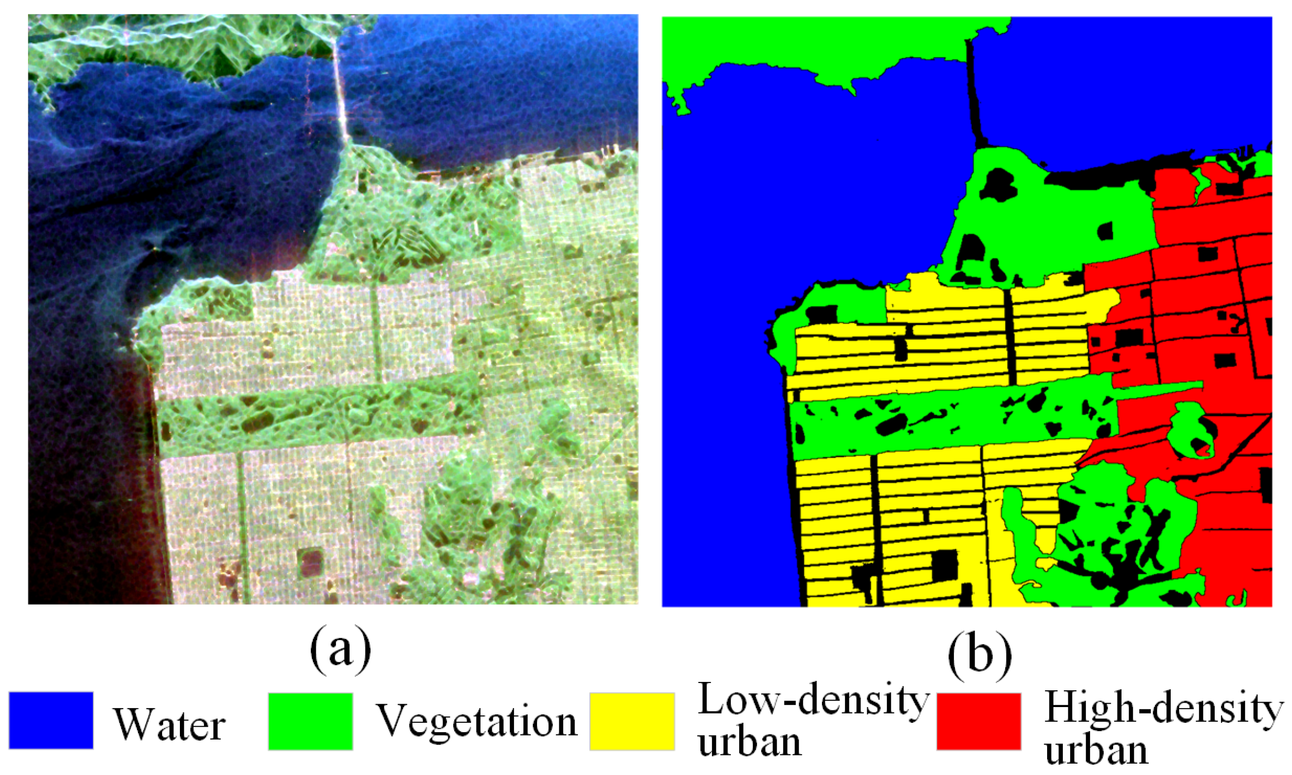
• The San Francisco dataset was acquired by National Aeronautics and Space Administration (NASA)/Jet Propulsion Laboratories (JPL) Airborne Synthetic Aperture Radar (AIRSAR) over the San Francisco area in the United States. It, with $823\times 850$ pixels, comprises four land cover categories: water, vegetation, low-density urban and high-density urban regions. Its Pauli pseudocolor image and ground truth map is shown in Figure 5a,b, respectively, where black regions in the latter represent background. The black areas in the ground truth map indicate the background.
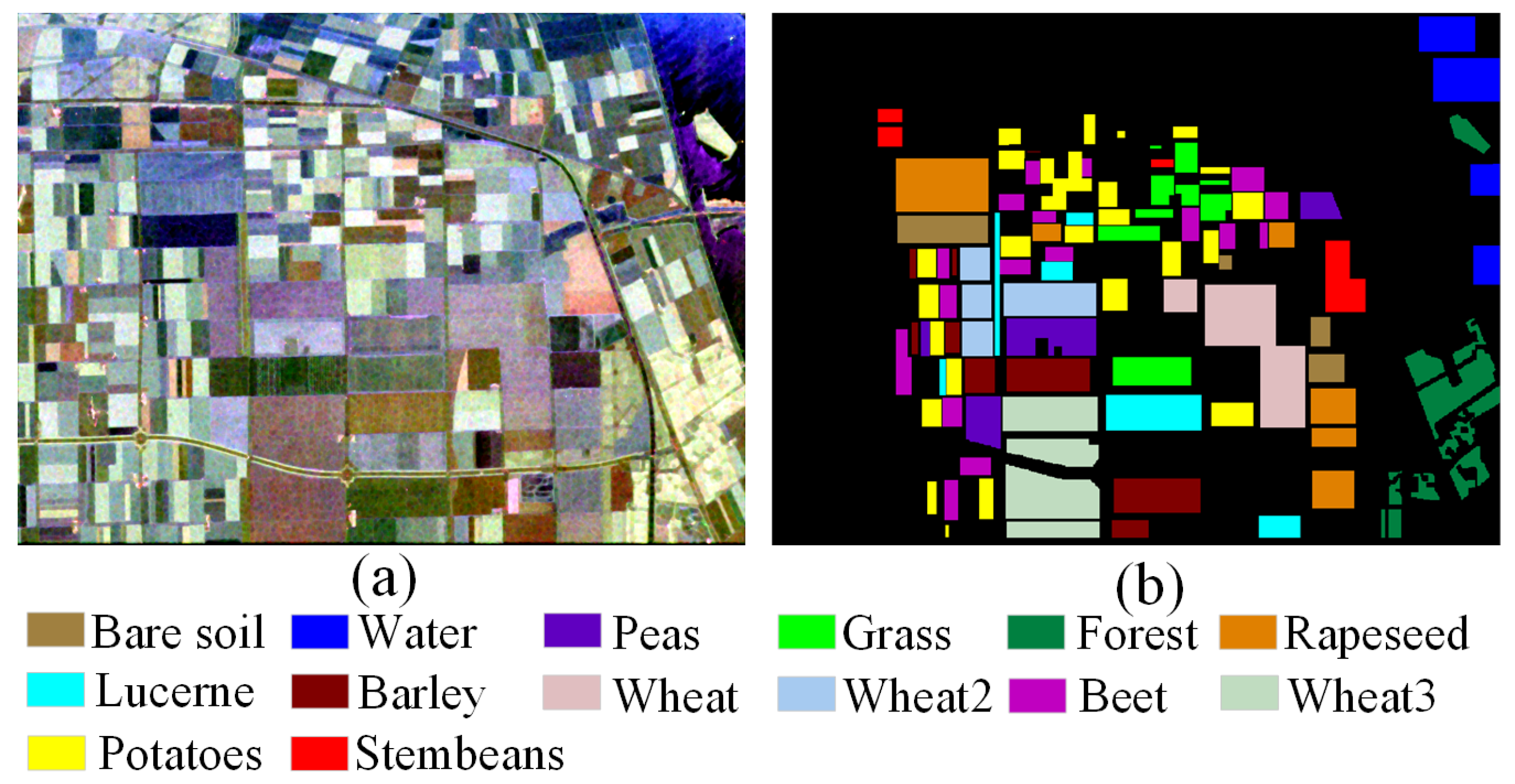
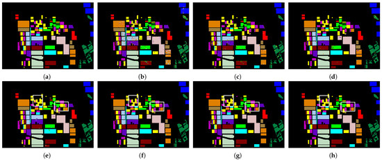
• The Flevoland dataset with $750\times 1024$ pixels was acquired over Flevoland in the Netherlands by NASA/JPL AIRSAR. As shown in Figure 6a, it encompasses 14 land cover types including bare soil, steam beans, peas, grass, forest, rapeseed, lucerne, barely, wheat, wheat2, beet, wheat3, potatoes, and water. Its ground truth map is presented in Figure 6b.
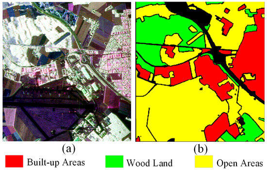
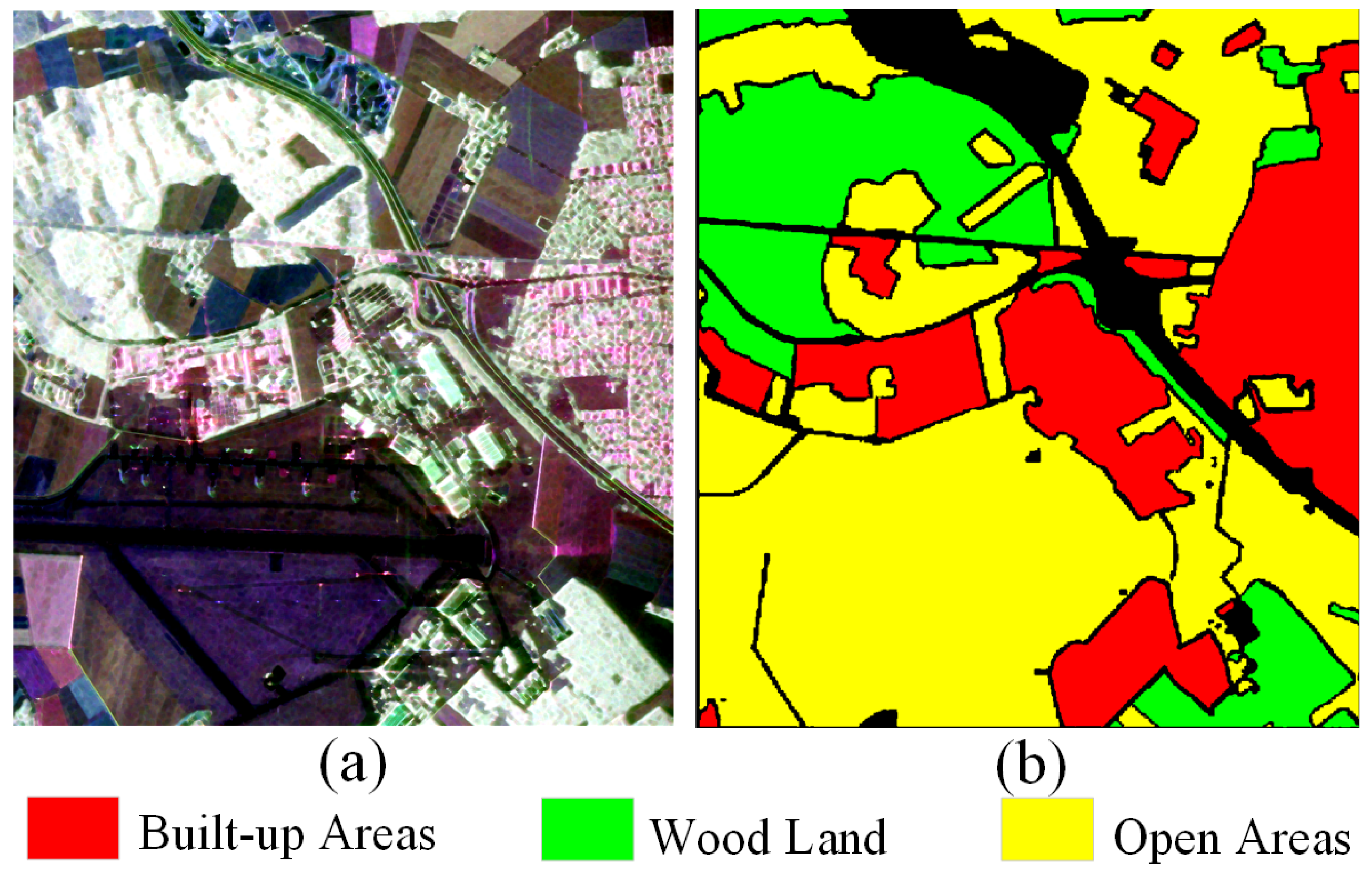
• The Oberpfaffenhofen dataset was collected over Oberpfaffenhofen area of the Germany using the Experimental Synthetic Aperture Radar (E-SAR) airborne platform. As shown in Figure 7a, it consists of $1300\times 1200$ pixels, covering three categories: built-up areas, wood land, along with open areas. The ground truth map is shown in Figure 7b.

The classification performance of all experiments was evaluated in terms of overall accuracy (OA), average accuracy (AA), and Kappa coefficient (Kappa). OA represents the ratio of the number of correctly predicted sample points in the image to the total number of predicted points. AA calculates the average classification accuracy for each category and pays attention to the classification balance for each category. Kappa is a statistical indicator used to evaluate the consistency of classification. Its value ranges from 0 to 1. The higher the value, the better the classification result and the higher the consistency. The above-mentioned Evaluation Metrics can be expressed as follows:

$$OA={\displaystyle \frac{{\sum }_{i=1}^Q{P}_{ii}}{N}}$$

(25)

$$AA={\displaystyle \frac{1}{Q}}\sum _{i=1}^Q{\displaystyle \frac{P_{ii}}{{\sum }_{j=1}^Q{P}_{ij}}}$$

(26)

$$Kappa={\displaystyle \frac{OA-p_e}{1-p_e}},p_e={\displaystyle \frac{{\sum }_{i=1}^Q\left({\sum }_{j=1}^Q{P}_{ij}\right)·\left({\sum }_{j=1}^Q{P}_{ji}\right)}{N^2}}$$

(27)

where $P_{ij}$ represents the element at the i-th row and j-th column of the confusion matrix.

3.3. Comparative Experiments

In this section, we employ both quantitative and qualitative methods to verify the effectiveness of the MAE-CV-GUNet model. This paper conducts classification experiments on three datasets and compares the MAE-CV-GUNet model with six other models: CNN [17], CV-3D-CNN [23], HybridCVNet [24], MSSP-GCN [32], DMSGer [29], and g-U-Net [40]. Among them, CV-3D-CNN and HybridCVNet are CV networks, MSSP-GCN and DMSGer are multiscale GCNs, and g-U-Net is a graph U-Net network.

3.3.1. Classification Results on the San Francisco Dataset

Table 3. Quantitative comparison on San Francisco dataset.

CLasses	CNN	CV-3D-CNN	HybridCVNet	MSSP-GCN	DMSGer	g-U-Net	Ours
Ocean	97.43	99.58	99.76	99.07	99.61	99.31	99.74
Vegetation	90.89	95.56	96.74	93.28	94.75	94.45	97.24
Low-density urban	90.67	93.44	93.38	97.25	98.23	98.75	98.93
High-density urban	88.50	84.45	91.25	95.93	96.30	97.85	98.76
OA (%)	93.46	95.33	96.72	96.94	97.75	97.85	98.88
AA (%)	91.90	93.26	95.28	96.38	97.22	97.59	98.67
Kappa (%)	90.57	93.26	96.72	95.58	96.74	96.91	98.37

shows the quantitative classification results on the San Francisco dataset, where the best values for each metric are shown in bold. From the experimental results, it can be seen that the classification performance of the MAE-CV-GUNet model is closely related to its ability to utilize CV information and local as well as global features. The real-valued CNN converted complex inputs into real numbers for processing, resulting in the loss of phase information. Moreover, due to the limited receptive field of two-dimensional convolution, its classification performance was rather limited, with an OA of only 93.46%. In contrast, CV-3D-CNN directly used complex numbers in the input layer and convolution kernels, preserving the phase information and making fuller use of the characteristics of complex numbers. As a result, it outperformed real-valued CNN by 1.87%, 1.36%, and 2.69% respectively in the OA, AA, and Kappa metrics. HybridCVNet further extracted different complex features through a multi-branch structure, and by leveraging a deeper network to indirectly capture global context information, it can achieve superior classification performance compared to CNN and CV-3D-CNN.

To break through the limitations of local modeling, the MSSP-GCN and DMSGer methods utilized the graph structure to explicitly capture context information at different scales, thereby effectively integrating local and global features. They outperformed the CNN and 3D-CV-CNN models that only consider local characteristics in all evaluation metrics. However, MSSP-GCN and DMSGer still operated independently when extracting features of different scales, and the feature fusion method was also relatively simple. In contrast, g-U-Net adopts a hierarchical encoder-decoder structure, which can extract and fuse multiscale information layer by layer: the lower-level network captured detailed features, the higher-level network extracted abstract semantics, and then through upsampling and skip connections, the features at different levels were deeply integrated. This structure achieved 97.85%, 97.59%, and 96.91% on OA, AA, and Kappa respectively, significantly outperforming MSSP-GCN and DMSGer. MAE-CV-GUNet model successfully integrated the feature extraction of the complex domain and the local-global multiscale modeling capability. It achieved the best overall performance and higher accuracy in most land-cover categories. By integrating complex-domain feature extraction with local-global multiscale modeling, the MAE-CV-GUNet model achieved the best overall performance and higher accuracy in most land-cover categories.

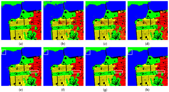
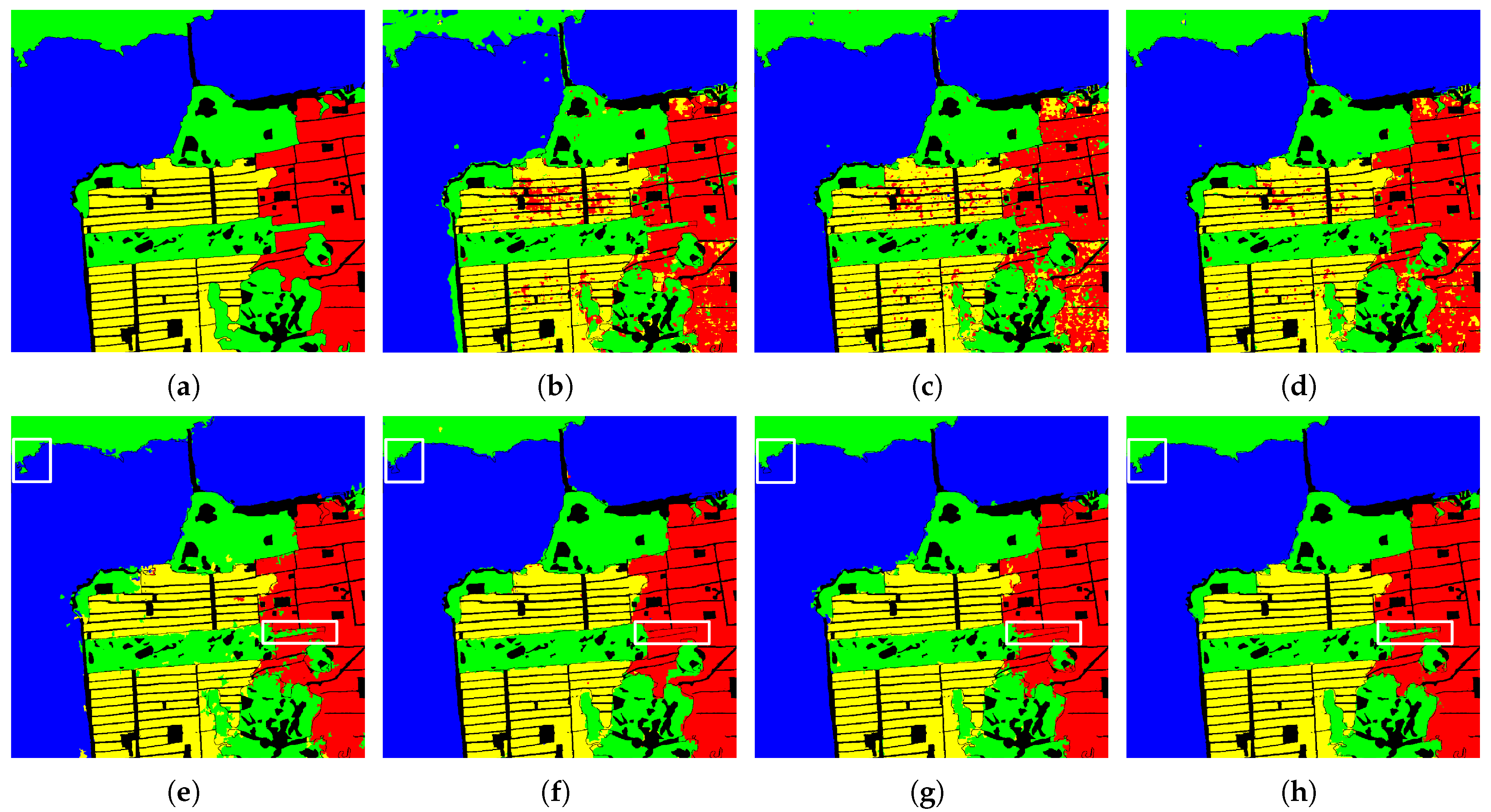
Figure 8 qualitatively compares the classification visualization results of different methods on the San Francisco dataset. As shown in Figure 8b–d, CNN, CV-3D-CNN, and HybridCVNet failed to effectively distinguish between “Low-density urban” and “High-density urban” areas and produced a large number of misclassified regions. This confusion is primarily attributed to their overlapping scattering mechanisms: despite their spatial distribution differences, low-density urban areas still exhibit strong double-bounce scattering from building-ground structures, similar to high-density areas, leading to highly similar polarimetric responses. Consequently, the classifier finds it difficult to discriminate between them. Nonetheless, CV-3D-CNN and HybridCVNet, which leverage CV information, showed fewer misclassifications overall and superior performance in distinguishing “vegetation” areas, underscoring the value of CV data in enhancing model discriminability. In Figure 8e–g, class confusion was significantly reduced, particularly showing improved regional consistency in the “Low-density urban” and “High-density urban” category. This result suggests that the integration of local and global information effectively enhances the discriminative power of the models, thereby improving the spatial consistency of the classification results. However, as highlighted by the white boxes in the Figure 8e–g, these methods struggled with inaccurate boundary localization, particularly for small-scale objects, where classification performance was also suboptimal. The MAE-CV-GUNet method illustrated in Figure 8h addressed the above issues, and had a better classification effect. It performs particularly well in the classification of small-scale objects. This demonstrates that the combination of CV information and multiscale spatial information effectively enhances the discriminative power of the extracted features, enabling MAE-CV-GUNet method to provide more accurate classification results when processing complex images.

3.3.2. Classification Results on the Flevoland Dataset

The quantitative evaluation results on the Flevoland dataset are presented in

Table 4. Quantitative comparison on Flevoland dataset.

CLasses	CNN	CV-3D-CNN	HybridCVNet	MSSP-GCN	DMSGer	g-U-Net	Ours
Stembeans	97.17	99.46	99.64	99.49	99.79	99.07	99.51
Peas	82.86	95.14	98.44	97.31	97.09	98.62	99.73
Forest	92.95	96.58	97.01	99.53	99.23	99.58	100
Lucerne	94.93	96.18	97.49	95.87	96.97	97.76	99.45
Wheat	92.70	98.05	96.56	99.45	99.55	99.71	99.96
Beet	89.26	95.58	97.04	87.63	94.15	94.48	98.21
Potatoes	89.50	95.02	97.39	97.36	96.42	96.40	98.04
Bare soil	95.75	92.54	99.19	97.72	99.01	99.99	99.99
Grass	87.16	92.07	93.28	95.73	98.95	99.10	99.39
Rapeseed	84.83	93.36	97.68	99.35	98.63	99.31	99.86
Barley	92.87	91.35	97.61	98.39	99.01	97.79	99.73
Wheat2	74.58	88.12	96.72	96.06	97.74	99.44	99.68
Wheat3	97.23	97.09	98.89	99.12	98.46	99.87	100
Water	96.57	99.83	99.87	99.91	99.99	99.99	100
OA (%)	90.52	95.06	97.56	97.39	98.08	98.51	99.47
AA (%)	90.60	95.03	97.63	97.35	98.21	98.64	99.54
Kappa (%)	89.71	94.64	97.56	97.17	97.91	98.38	99.43

, where the highest value for each metric is highlighted in bold. As shown, the classification performance of CNN is significantly lower than that of the CV networks CV-3D-CNN and HybridCVNet. For the challenging “Wheat2” category, CV-3D-CNN and HybridCVNet effectively modeled CV scattering characteristics, achieving accuracy improvements of 13.54% and 22.14%, respectively. It fully demonstrates the critical role of complex information in distinguishing terrains with similar scattering mechanisms. On the other hand, multiscale GCN methods MSSP-GCN, DMSGer, and g-U-Net, generally outperformed CNN-based approaches in most terrain categories, as they can simultaneously model local structures and global contextual relationships. However, for the “Beet” category, which is dominated by volume scattering, exhibits dense plant arrangement, and has limited morphological and textural variation, the discriminability of both local and global features is reduced, leading to moderate performance of these multiscale GCN methods. In contrast, the effectiveness of CV-3D-CNN and HybridCVNet in this category underscores the critical importance of phase information for identifying “Beet”. The MAE-CV-GUNet model, by integrating CV feature modeling and multiscale contextual awareness, achieves over 98% accuracy in both of the aforementioned challenging categories, “Wheat2” and “Beet”. Furthermore, our method attains the highest classification accuracy across all 12 categories, including Peas, Forest, Lucerne, Wheat, Beet, Potatoes, Bare soil, Rapeseed, Barley, Wheat2, Wheat3, and Water. Finally, the OA, AA, and Kappa of the MAE-CV-GUNet method reach 99.47%, 99.54%, and 99.43%, respectively, all surpassing the other six comparison methods. These results further confirm the effectiveness and advancement of MAE-CV-GUNet method in complex PolSAR image classification tasks.

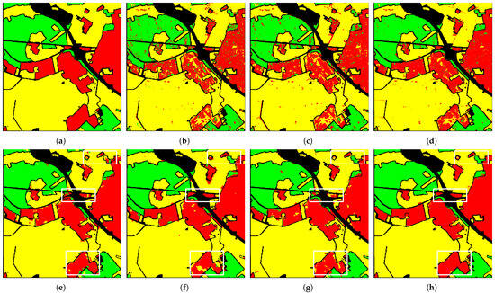
Figure 9 qualitatively presents the visualization results of different classification models on the Flevoland dataset. As shown in Figure 9b–d, the CV methods CV-3D-CNN and HybridCVNet significantly reduced misclassification areas and improved the spatial continuity of ground objects compared to the CNN. As shown in Figure 9e–g, by integrating local structures and global contextual information, the multiscale GCN methods MSSP-GCN, DMSGer, and g-U-Net achieved classification results with superior regional consistency and significantly fewer misclassifications in homogeneous areas. Although the overall classification performance of these methods surpassed that of the CNN-based models, certain misclassifications persisted along category boundaries. The regions marked by white boxes indicate that the three models exhibited limited discriminative ability between “Potatoes” and “Beet,” consistently misclassifying “Beet” as “Potatoes.” In contrast, the proposed MAE-CV-GUNet method in Figure 9h showed almost no obvious misclassification areas, demonstrating optimal boundary preservation capability and the most visually consistent classification result. These findings indicate that the MAE-CV-GUNet method effectively mitigates inter-class confusion while exhibiting excellent performance in both boundary preservation and regional consistency.

3.3.3. Classification Results on the Oberpfaffenhofen Dataset

Table 5. Quantitative comparison on Oberpfaffenhofen dataset.

CLasses	CNN	CV-3D-CNN	HybridCVNet	MSSP-GCN	DMSGer	g-U-Net	Ours
Built-up Areas	78.89	84.07	89.96	93.67	94.98	95.49	98.43
Wood Land	90.83	91.95	96.33	95.00	96.72	96.93	99.36
Open Areas	97.63	97.47	97.90	97.78	98.23	98.84	98.27
OA (%)	91.67	93.08	95.62	96.22	97.14	97.64	99.07
AA (%)	89.12	91.16	94.73	95.48	96.64	97.09	99.02
Kappa (%)	85.65	88.10	95.62	93.55	95.11	95.97	98.43

presents the quantitative evaluation results of different classification models on the Oberpfaffenhofen dataset, where the highest value for each metric is shown in bold. The experimental data indicate that both CV-3D-CNN and HybridCVNet outperformed the CNN, which is consistent with the findings from the San Francisco and Flevoland datasets, further confirming the effectiveness of CV information in improving classification performance. Meanwhile, the multiscale graph convolution methods, by integrating local and global information, also achieved better overall performance than CNN-based approaches. The experimental data indicated that the six comparative methods generally demonstrated limited discriminative capability for the “Built-up Areas” category, with classification accuracy ranging from 78.89% to 95.49% for this class. In contrast, the proposed method achieved an improved accuracy of 98.43% for this category. Notably, the MAE-CV-GUNet model also attained competitive classification performance in the other two land cover categories. The proposed Method MAE-CV-GUNet achieved 99.07%, 99.02%, and 98.43% in OA, AA, and Kappa, comprehensively outperforming all six comparative methods. These results validate the effectiveness and robustness of the proposed MAE-CV-GUNet approach in PolSAR classification tasks.

The qualitative results of different methods on the Oberpfaffenhofen dataset are shown in Figure 10. We observed distinct misclassification across various land cover categories with different methods. A particularly pronounced confusion was identified between “Built-up Areas” and “Wood Land” categories. Although the methods in Figure 10e–g demonstrated improved regional consistency compared to Figure 10b–d and achieved reduced misclassification areas, their classification performance at land cover boundaries remained unsatisfactory (as highlighted by the white boxes). Conversely, MAE-CV-GUNet exhibited outstanding performance, showing high spatial agreement with the ground truth labels. MAE-CV-GUNet particularly excelled in preserving detailed features and achieving accurate boundary localization.

4. Discussion

From the classification results on the three PolSAR datasets, we can see that the MAE-CV-GUNet model achieves the highest OA, AA, and Kappa values. In the visual classification maps, it also presents good boundary consistency and robustness to noise, and correctly classifies most categories. These results verify the effectiveness of the MAE-CV-GUNet model for PolSAR image classification.

Building on these results, we further analyze how several key design choices affect the performance of the proposed model. To evaluate the impact of CV operations, the MSA module, HiAS configuration, and training sample proportion, this section conducted a series of ablation experiments on the San Francisco dataset. We also compared the training time across different models, with the San Francisco-RS2 dataset from the RADARSAT-2 satellite serving to validate their generalization capability.

4.1. Model Ablation Study

MAE-CV-GUNet has two main innovations, namely the CV-GCN and MSA model. To evaluate their effectiveness, we designed three sets of ablation experiments: GUNet, CV-GUNet, and MAE-CV-GUNet models. The obtained OA, AA, and Kappa are shown in

Table 6. Ablation study results in three datasets.

Method	San Francisco			Flevoland			Oberpfaffenhofen
	OA	AA	Kappa	OA	AA	Kappa	OA	AA	Kappa
GUNet	97.11	96.68	95.83	98.25	98.35	98.10	96.48	96.43	94.04
CV-GUNet	98.37	98.09	97.66	98.46	98.58	98.33	97.34	97.22	95.31
MAE-CV-GUNet	98.88	98.67	98.37	99.47	99.54	99.43	99.07	99.02	98.43

, with the best values shown in bold. GUNet replaced the CV-GCN in MAE-CV-GUNet with RV-GCN and removed the MSA module, using the features of the final decoder layer for classification. The CV-GUNet model is a CV GUNet network without the MSA module. Table 6 demonstrates progressive performance improvements across methods GUNet, CV-GUNet, and MAE-CV-GUNet on all three datasets. On the San Francisco dataset, CV-GUNet outperformed GUNet with gains of 1.26% (OA), 1.41% (AA), and 1.83% (Kappa). Similar improvements were observed on the Flevoland (0.21% OA, 0.23% AA, 0.23% Kappa) and Oberpfaffenhofen datasets (0.86% OA, 0.79% AA, 1.27% Kappa). These consistent enhancements confirm that CV information effectively strengthens model discriminability and overall classification performance. Furthermore, MAE-CV-GUNet achieved additional accuracy gains over CV-GUNet: 0.51% (OA), 0.58% (AA), and 0.71% (Kappa) on San Francisco; 1.01%, 0.96%, and 1.1% on Flevoland; and 1.73%, 2.2%, and 3.12% on Oberpfaffenhofen, respectively. These results validate the advantage of MSA module in multiscale information fusion, where enhanced feature representation at critical scales significantly improves discrimination accuracy for complex land cover categories.

4.2. HiAS Configuration

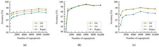
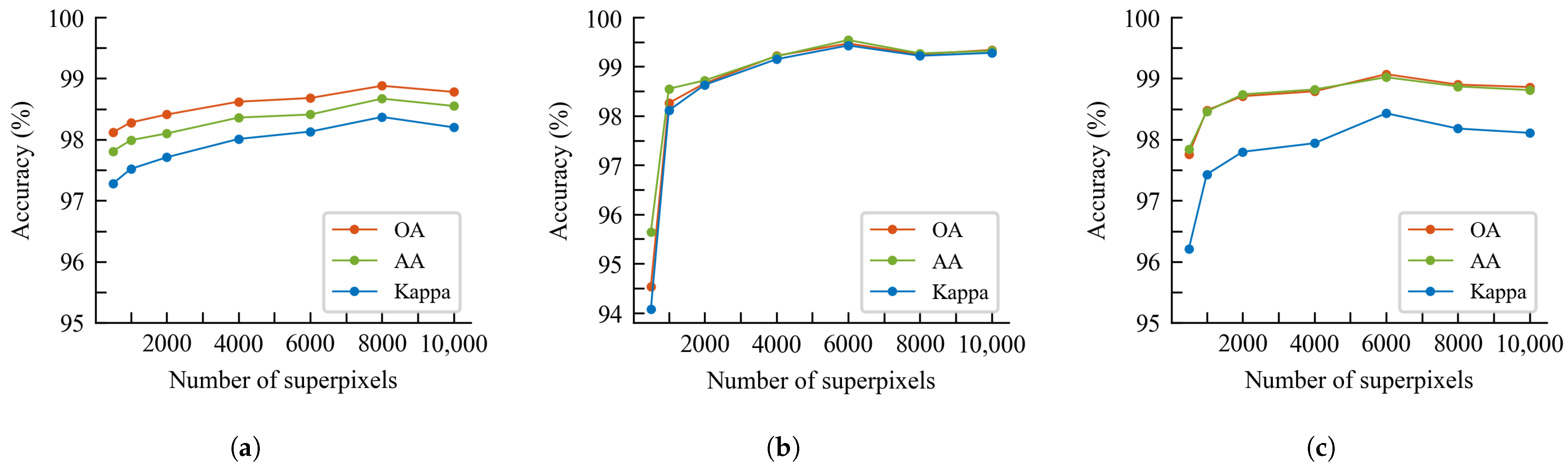
In the section, we evaluated how structure parameters in HiAS affect classification performance, with particular focus on hierarchical superpixel count and edge weight $\vartheta$. Due to the large size of the PolSAR images, HiAS is set to 3 layers. The number of superpixels in each layer is set in a decreasing manner, with the number of superpixels in the next layer being half of that of the previous layer. We evaluated the impact of first-layer superpixel quantity on classification performance by measuring OA, AA, and Kappa variations across three datasets using superpixel numbers of 500, 1000, 2000, 4000, 6000, 8000, and 10,000. Figure 11 reveals distinct responses to superpixel quantity across datasets. The category-rich Flevoland dataset showed higher sensitivity to this parameter, while San Francisco and Oberpfaffenhofen maintained relatively stable classification performance. The San Francisco dataset achieved optimal results with 8000 first-layer superpixels, reaching values of 98.88%, 98.67%, and 98.37% for OA, AA, and Kappa respectively. Flevoland attained its peak performance with 6000 superpixels, recording corresponding values of 99.47%, 99.54%, and 99.43%. Oberpfaffenhofen required 6000 first-layer superpixels to achieve its optimal OA, AA, and Kappa values of 99.07%, 99.02%, and 98.43%. Thus, the first-layer superpixel numbers for the San Francisco, Flevoland and Oberpfaffenhofen datasets were set to 8000, 6000, and 6000, respectively.

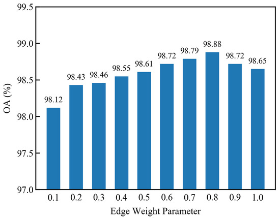
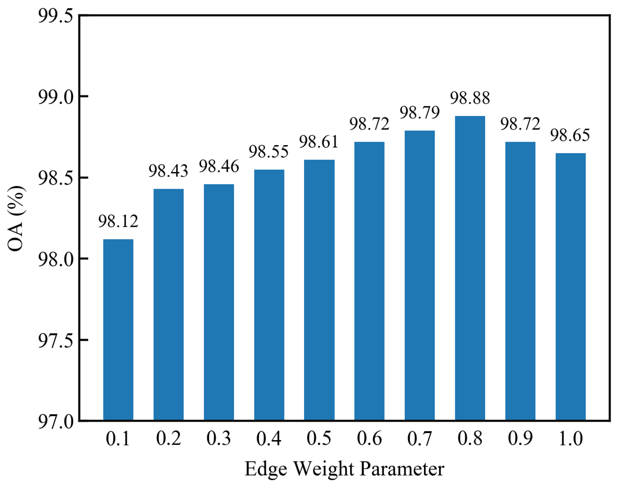
To determine the optimal edge weight $\vartheta$, we examined the variation of OA with edge weight, as shown in Figure 12. Increasing the edge weight from 0.1 to 0.2 boosted OA from 98.12% to 98.43%. This performance leap confirms the complementary characteristics of the color distance and modified Wishart distance metrics. OA then rose gradually to its peak of 98.88% within the 0.2–0.8 weight range, demonstrating optimal balance between both metrics. Further increasing the weight beyond 0.8 reduced OA, indicating impaired model generalization due to excessive color distance dominance in feature fusion. These findings support our selection of 0.8 as the optimal edge weight $\vartheta$.

4.3. Training Sample Ratio

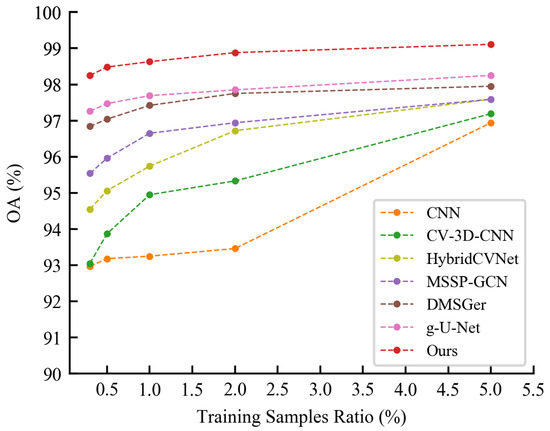
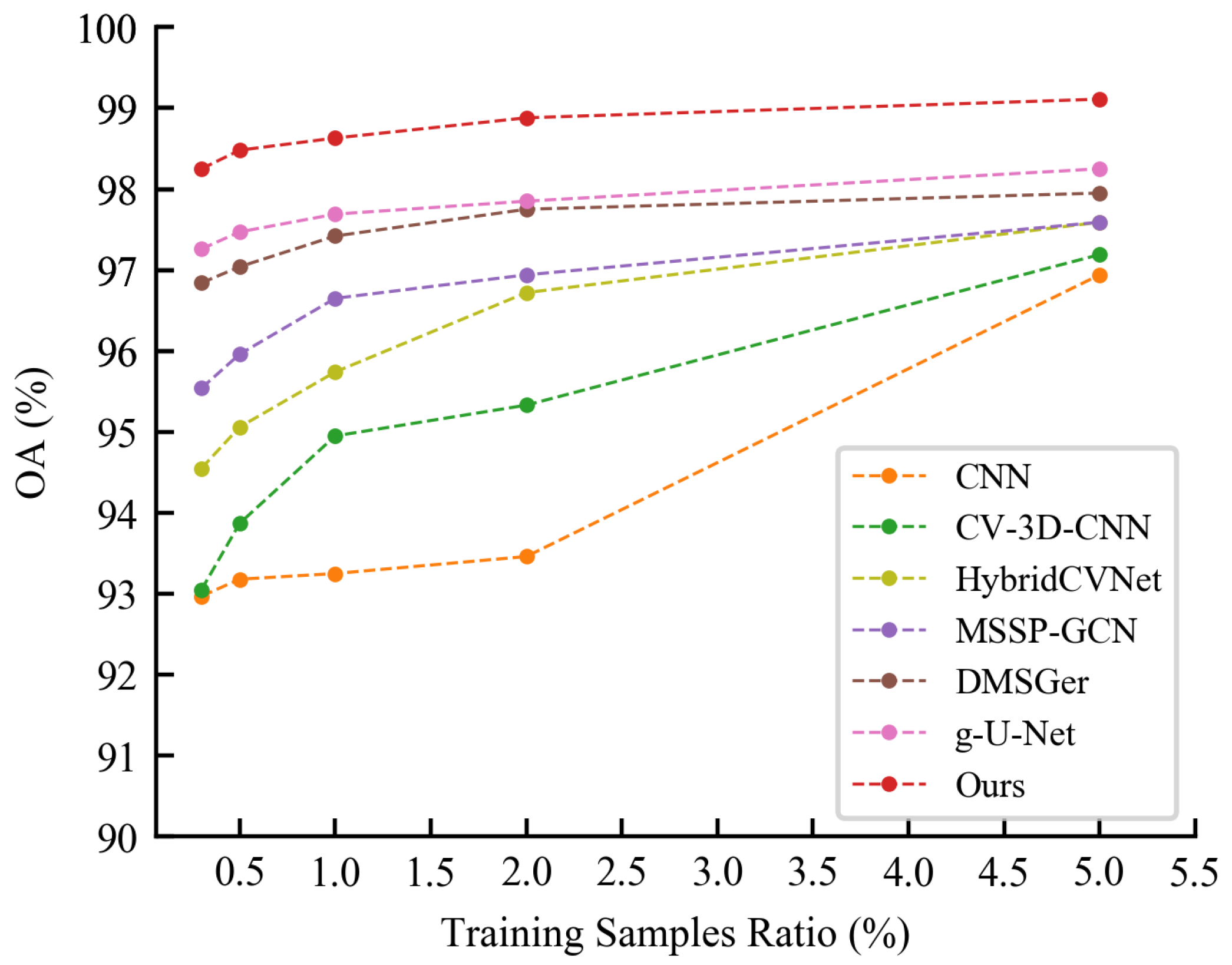
In this experiment, we investigated the impact of varying the proportion of labeled samples per class in the training set on different methods. When the proportion of training samples is set at 0.25%, 0.5%, 1.0%, 2.0% and 5.0%, the changes in OA are shown in Figure 13. The CV-3D-CNN and HybridCVNet models, which use PolSAR phase information, consistently performed better than the CNN model. This result confirms the value of CV features for improving classification. Graph-based models MSSP-GCN, DMSGer, g-U-Net, and our model showed stronger robustness to sample size changes. These models have fewer parameters than CNN-based approaches. They maintained good accuracy even with very few training samples. Our model achieved the best accuracy at all sample proportions. It effectively combines CV phase features with multiscale spatial context. This demonstrates its strong adaptability and stable performance across different data volumes.

4.4. Inference Time

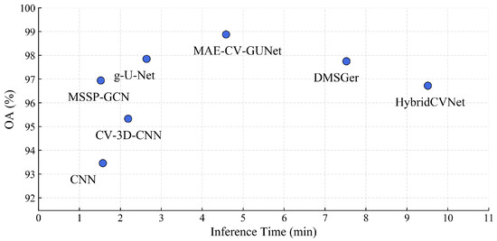
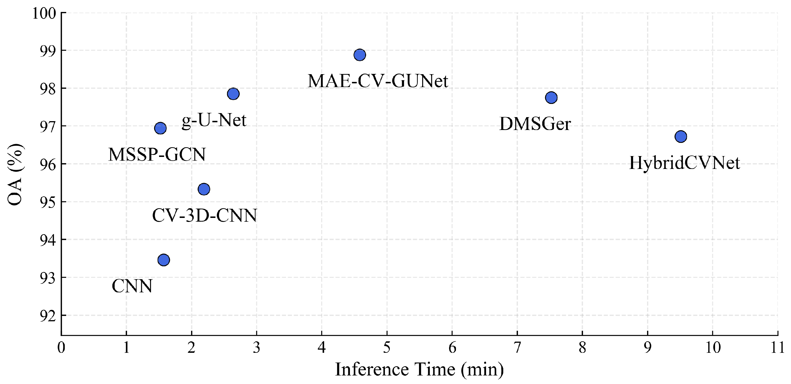
To objectively evaluate the overall performance of the MAE-CV-GUNet model, we conducted a quantitative analysis of the inference efficiency of different methods, with results shown in Figure 14. The structurally simpler CNN and MSSP-GNN achieved the shortest inference times, yet their classification accuracy remained at a moderate level among all models. The two CV models, CV-3D-CNN and HybridCVNet, required longer inference times than CNN, reflecting the higher computational complexity typically associated with CV operations. Although the DMSGer model attained higher classification accuracy, its structural complexity led to a substantial increase in inference time, indicating that its performance gain came at the cost of efficiency. The proposed CV model MAE-CV-GUNet achieved inference efficiency between DMSGer and g-U-Net. While not optimal in speed, it attained the highest classification accuracy among all methods. These results demonstrate that MAE-CV-GUNet achieves an effective balance between computational efficiency and classification performance.

4.5. Generalization Study

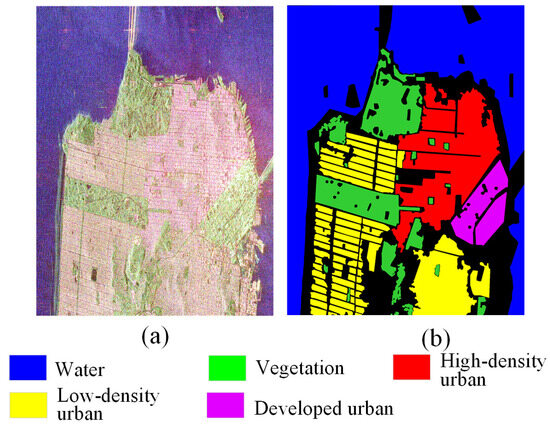
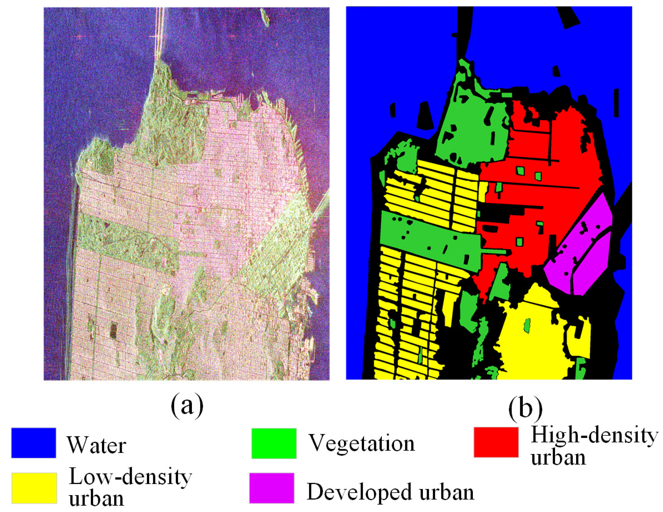
To investigate the generalization ability of the proposed model, we further conduct experiments on a spaceborne SAR dataset. The San Francisco-RS2 dataset was a C-band spaceborne SAR image of the San Francisco area in the United States acquired by the RADARSAT-2 system. The image has a size of 1800 × 1380 pixels and contains five land-cover classes: Water, Vegetation, Low-density urban, High-density urban, and Developed urban, as shown in Figure 15a,b.

Table 7. Quantitative comparison on San Francisco-RS2 dataset.

CLasses	CNN	CV-3D-CNN	HybridCVNet	MSSP-GCN	DMSGer	g-U-Net	Ours
Ocean	99.93	99.93	99.94	99.57	98.76	99.99	99.71
Vegetation	88.92	88.02	90.79	91.82	92.45	93.74	96.37
Low-density urban	80.24	88.13	89.64	95.97	97.93	97.52	98.87
High-density urban	76.43	89.85	92.53	95.84	98.45	98.08	99.31
Development urban	70.78	88.30	87.42	86.47	98.65	99.61	99.99
OA (%)	89.66	93.97	95.01	96.68	97.71	98.46	99.06
AA (%)	83.26	90.85	92.06	93.94	97.25	97.79	98.85
Kappa (%)	85.10	91.32	95.01	95.22	96.72	97.65	98.65

shows the evaluation metrics, where the best values are in bold. The best value for each metric is indicated in bold. The CNN model delivers limited performance on the San Francisco-RS2 dataset, with OA below 90%. Both CV-3D-CNN and HybridCVNet, which are capable of encoding complex-valued information, achieve OA values exceeding 93%, and demonstrate satisfactory performance in discriminating more challenging categories such as “High-density urban” and “Development urban”. Graph-based models including MSSP-GCN, DMSGer, and g-U-Net perform well across all categories by incorporating both local and global structural information, attaining OA values above 96%. Meanwhile, our proposed model, which simultaneously encodes complex-valued information along with local and global structures, achieves superior classification accuracy in most categories compared to other methods, reaching an OA of 99.06%. This result validates the effectiveness of our proposed model on spaceborne SAR data.

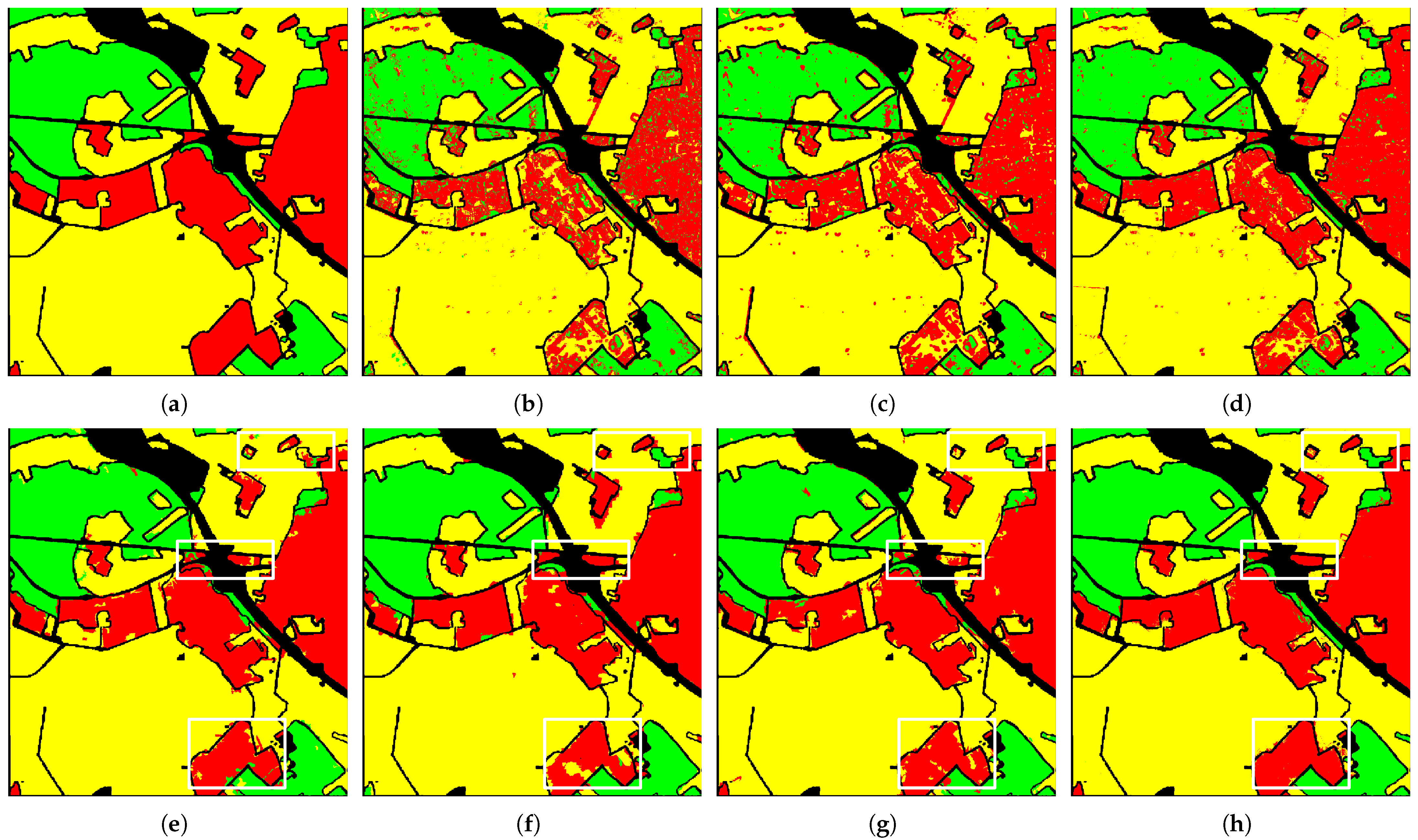
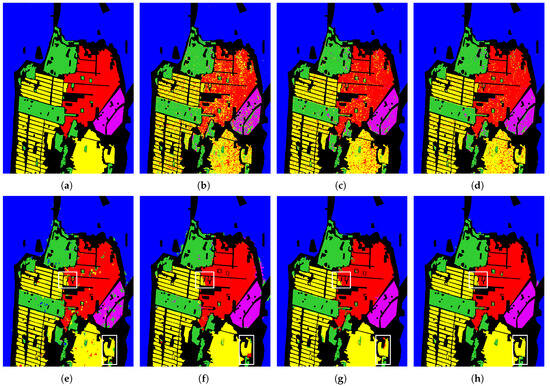
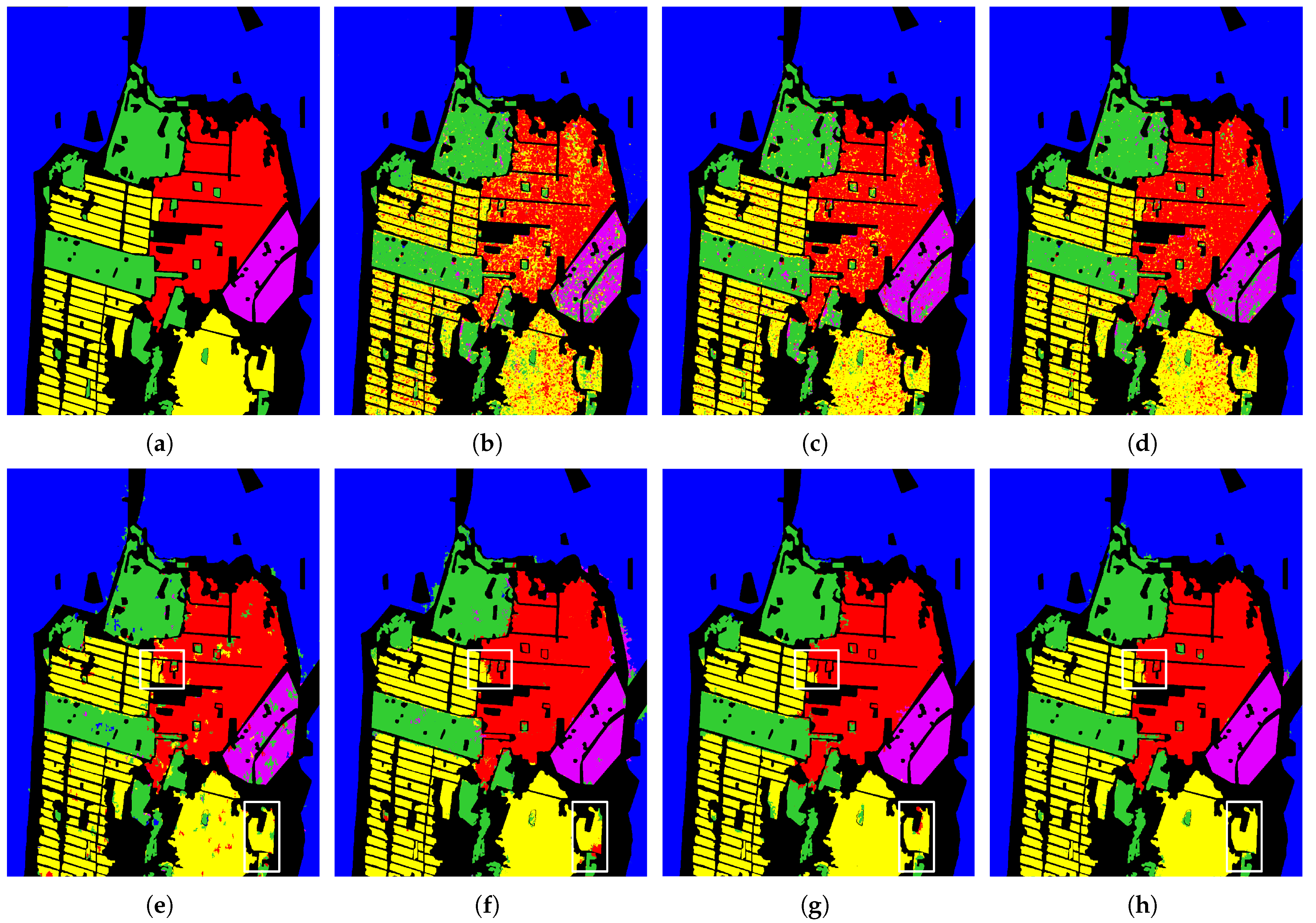
As shown in Figure 16, the qualitative classification results are consistent with the quantitative analysis in Table 7. Figure 16b–d exhibit numerous scattered misclassification regions. While these dispersed errors are reduced in Figure 16e–g, notable misclassifications persist along the boundaries. In contrast, our proposed model (Figure 16h) demonstrates superior boundary preservation and significantly fewer misclassified areas, further validating its effectiveness for spaceborne SAR imagery.

5. Conclusions

In this paper, a novel MAE-CV-GUNet framework has been proposed for PolSAR image classification. This algorithm effectively utilizes both the CV information and multiscale spatial characteristics in PolSAR images. In MAE-CV-GUNet, a CV-GCN is proposed to effectively exploit and use both amplitude and phase information, where the graph convolution layer, batch normalization layer, and activation layer are all implemented in complex form to fully exploit both amplitude and phase information in PolSAR data. By designing a CV-GUNet to integrate multiple CV-GCN, the model has effectively extracted multiscale features, enabling simultaneous learning of both local and global characteristics. In addition, the proposed MAE-CV-GUNet introduces a multiscale attention mechanism, thus achieving adaptive integration of multiscale features. We evaluated the proposed MAE-CV-GUNet method by conducting experiments on three real PolSAR images. Results demonstrate that MAE-CV-GUNet possesses strong capabilities in CV feature extraction and multiscale feature learning, significantly improving classification performance. In the future, we will focus on developing lightweight complex-valued network architectures to enhance computational efficiency while maintaining performance advantages. We also plan to explore the transferability of our model to other PolSAR interpretation tasks, such as target detection and change detection. Finally, we note that the method relies on pre-computed superpixel segmentation, so the overall performance is affected by its quality, and we will investigate more adaptive strategies in future work.

References

- Yin, Q.; Gao, L.; Zhou, Y.; Li, Y.; Zhang, F.; López-Martínez, C.; Hong, W. Coherence Matrix Power Model for Scattering Variation Representation in Multi-Temporal PolSAR Crop Classification. IEEE J. Sel. Top. Appl. Earth Obs. Remote Sens. 2024, 17, 9797–9810. [Google Scholar] [CrossRef] [Scilit]
- Corbane, C.; Kato, S.; Iwao, K.; Sabo, F.; Politis, P.; Pesaresi, M.; Kemper, T. Leveraging ALOS-2 PALSAR-2 for Mapping Built-Up Areas and Assessing Their Vertical Component. IEEE J. Sel. Top. Appl. Earth Obs. Remote Sens. 2020, 13, 6473–6483. [Google Scholar] [CrossRef] [Scilit]
- Zhang, C.; Gao, G.; Zhang, X.; Li, H.; Liu, T.; Zhang, Z.; Li, G. An Overview of Polarized Synthetic Aperture Radar Ship Detection: From traditional methods to artificial intelligence. IEEE Geosci. Remote Sens. Mag. 2025, 2–37. [Google Scholar] [CrossRef] [Scilit]
- Ren, B.; Hou, B.; Zhao, J.; Jiao, L. Unsupervised Classification of Polarimetirc SAR Image Via Improved Manifold Regularized Low-Rank Representation With Multiple Features. IEEE J. Sel. Top. Appl. Earth Obs. Remote Sens. 2017, 10, 2–37. [Google Scholar] [CrossRef] [Scilit]
- Dey, S.; Bhattacharya, A.; Ratha, D.; Mandal, D.; Frery, A.C. Target Characterization and Scattering Power Decomposition for Full and Compact Polarimetric SAR Data. IEEE Trans. Geosci. Remote Sens. 2021, 59, 3981–3998. [Google Scholar] [CrossRef] [Scilit]
- Sabry, R. Hybrid Products for Enhanced and Unified Full and Compact Polarimetric SAR Data Exploitations. IEEE J. Sel. Top. Appl. Earth Obs. Remote Sens. 2025, 18, 3981–3998. [Google Scholar] [CrossRef] [Scilit]
- Freeman, A.; Durden, S.L. A three-component scattering model for polarimetric SAR data. IEEE Trans. Geosci. Remote Sens. 1998, 36, 963–973. [Google Scholar] [CrossRef] [Scilit]
- Yamaguchi, Y.; Moriyama, T.; Ishido, M.; Yamada, H. Four-component scattering model for polarimetric SAR image decomposition. IEEE Trans. Geosci. Remote Sens. 2005, 43, 1699–1706. [Google Scholar] [CrossRef] [Scilit]
- Hanis, D.; Hadj-Rabah, K.; Belhadj-Aissa, A.; Pallotta, L. Dominant Scattering Mechanism Identification From Quad-Pol-SAR Data Analysis. IEEE J. Sel. Top. Appl. Earth Obs. Remote Sens. 2024, 17, 14408–14420. [Google Scholar] [CrossRef] [Scilit]
- Masjedi, A.; Valadan Zoej, M.J.; Maghsoudi, Y. Classification of Polarimetric SAR Images Based on Modeling Contextual Information and Using Texture Features. IEEE Trans. Geosci. Remote Sens. 2016, 54, 932–943. [Google Scholar] [CrossRef] [Scilit]
- Samat, A.; Li, E.; Wang, W.; Liu, S.; Liu, X. HOLP-DF: HOLP Based Screening Ultrahigh Dimensional Subfeatures in Deep Forest for Remote Sensing Image Classification. IEEE J. Sel. Top. Appl. Earth Obs. Remote Sens. 2022, 15, 8287–8298. [Google Scholar] [CrossRef] [Scilit]
- Song, W.; Wu, Y.; Xiao, X. Nonstationary PolSAR Image Classification by Deep-Features-Based High-Order Triple Discriminative Random Field. IEEE Geosci. Remote Sens. Lett. 2021, 18, 1406–1410. [Google Scholar] [CrossRef] [Scilit]
- Hua, Q.; Ma, X.; Yang, X.; Zhang, Y.; Dai, Y. Swish-Cardioid CV-CNN: A Novel Complex-Valued Activation Framework for PolSAR Terrain Classification. IEEE Geosci. Remote Sens. Lett. 2025, 22, 1–5. [Google Scholar] [CrossRef] [Scilit]
- Ren, B.; Hua, C.; Hou, B.; Lv, J.; Yang, C.; Jiao, L. PDCNet: A Polarimetric Data-Enhanced Contrastive Learning Network for PolSAR Land Cover Classification. IEEE J. Sel. Top. Appl. Earth Obs. Remote Sens. 2025, 18, 10010–10025. [Google Scholar] [CrossRef] [Scilit]
- Gui, R.; Xu, X.; Yang, R.; Deng, K.; Hu, J. Generalized Zero-Shot Domain Adaptation for Unsupervised Cross-Domain PolSAR Image Classification. IEEE J. Sel. Top. Appl. Earth Obs. Remote Sens. 2022, 15, 270–283. [Google Scholar] [CrossRef] [Scilit]
- Kamada, S.; Ichimura, T. Automatic extraction of road networks by using teacher-student adaptive structural deep belief network and its application to landslide disaster. IEEE J. Sel. Top. Appl. Earth Obs. Remote Sens. 2022, 15, 270–283. [Google Scholar] [CrossRef] [Scilit]
- Xu, R.; Zhang, S.; Dong, C.; Mei, S.; Zhang, J.; Zhao, Q. Lightweight Attention Refined and Complex-Valued BiSeNetV2 for Semantic Segmentation of Polarimetric SAR Image. Remote Sens. 2025, 17, 3527. [Google Scholar] [CrossRef] [Scilit]
- Zhou, Y.; Wang, H.; Xu, F.; Jin, Y.-Q. Polarimetric SAR Image Classification Using Deep Convolutional Neural Networks. IEEE Geosci. Remote Sens. Lett. 2016, 13, 1935–1939. [Google Scholar] [CrossRef] [Scilit]
- Chen, S.-W.; Tao, C.-S. PolSAR Image Classification Using Polarimetric-Feature-Driven Deep Convolutional Neural Network. IEEE Geosci. Remote Sens. Lett. 2018, 15, 627–631. [Google Scholar] [CrossRef] [Scilit]
- Hua, W.; Zhang, C.; Xie, W.; Jin, X. Polarimetric SAR Image Classification Based on Ensemble Dual-Branch CNN and Superpixel Algorithm. IEEE J. Sel. Top. Appl. Earth Obs. Remote Sens. 2022, 15, 2759–2772. [Google Scholar] [CrossRef] [Scilit]
- Lee, J.-S.; Grunes, M.R.; Pottier, E. Quantitative comparison of classification capability: Fully polarimetric versus dual and single-polarization SAR. IEEE Trans. Geosci. Remote Sens. 2021, 39, 2343–2351. [Google Scholar] [CrossRef] [Scilit]
- Zhang, Z.; Wang, H.; Xu, F.; Jin, Y.-Q. Complex-valued convolutional neural network and its application in polarimetric SAR image classification. IEEE Trans. Geosci. Remote Sens. 2017, 55, 7177–7188. [Google Scholar] [CrossRef] [Scilit]
- Tan, X.; Li, M.; Zhang, P.; Wu, Y.; Song, W.Y. Complex-Valued 3-D Convolutional Neural Network for PolSAR Image Classification. IEEE Geosci. Remote Sens. Lett. 2020, 17, 1022–1026. [Google Scholar] [CrossRef] [Scilit]
- Alkhatib, M.Q. PolSAR Image Classification Using a Hybrid Complex-Valued Network (HybridCVNet). IEEE Geosci. Remote Sens. Lett. 2024, 21, 1–5. [Google Scholar] [CrossRef] [Scilit]
- Yang, S.; Li, R.; Li, Z.; Meng, H.; Feng, Z.; He, G. Meta-Graph Representation Learning for PolSAR Image Classification. IEEE Trans. Geosci. Remote Sens. 2024, 62, 1–12. [Google Scholar] [CrossRef] [Scilit]
- Qin, A.; Shang, Z.; Tian, J.; Wang, Y.; Zhang, T.; Tang, Y.Y. Spectral–Spatial Graph Convolutional Networks for Semisupervised Hyperspectral Image Classification. IEEE Geosci. Remote Sens. Lett. 2019, 16, 241–245. [Google Scholar] [CrossRef] [Scilit]
- Mou, L.; Lu, X.; Li, X.; Zhu, X.X. Nonlocal Graph Convolutional Networks for Hyperspectral Image Classification. IEEE Trans. Geosci. Remote Sens. 2020, 58, 8246–8257. [Google Scholar] [CrossRef] [Scilit]
- Wan, S.; Gong, C.; Zhong, P.; Du, B.; Zhang, L.; Yang, J. Multiscale Dynamic Graph Convolutional Network for Hyperspectral Image Classification. IEEE Trans. Geosci. Remote Sens. 2020, 58, 3162–3177. [Google Scholar] [CrossRef] [Scilit]
- Yang, Y.; Tang, X.; Zhang, X.; Ma, J.; Liu, F.; Jia, X. Semi-Supervised Multiscale Dynamic Graph Convolution Network for Hyperspectral Image Classification. IEEE Trans. Neural Netw. Learn. Syst. 2024, 35, 6806–6820. [Google Scholar] [CrossRef] [Scilit]
- Gao, H.; Ji, S. Graph U-Nets. IEEE Trans. Pattern Anal. Mach. Intell. 2022, 44, 4948–4960. [Google Scholar] [CrossRef] [Scilit]
- Liu, F.; Wang, J.; Tang, X.; Liu, J.; Zhang, X. Adaptive Graph Convolutional Network for PolSAR Image Classification. IEEE Trans. Geosci. Remote Sens. 2022, 60, 1–14. [Google Scholar] [CrossRef] [Scilit]
- Cheng, J.; Zhang, F.; Xiang, D.; Yin, Q.; Zhou, Y. PolSAR Image Classification With Multiscale Superpixel-Based Graph Convolutional Network. IEEE Trans. Geosci. Remote Sens. 2022, 60, 1–14. [Google Scholar] [CrossRef] [Scilit]
- Wang, R.; Nie, Y.; Geng, J. Multiscale Superpixel-Guided Weighted Graph Convolutional Network for Polarimetric SAR Image Classification. IEEE J. Sel. Top. Appl. Earth Obs. Remote Sens. 2024, 17, 3727–3741. [Google Scholar] [CrossRef] [Scilit]
- Xiang, D.; Ban, Y.; Wang, W.; Su, Y. Adaptive superpixel generation for polarimetric SAR images with local iterative clustering and SIRV model. IEEE Trans. Geosci. Remote Sens. 2017, 55, 3115–31311. [Google Scholar] [CrossRef] [Scilit]
- Wang, W.; Xiang, D.; Ban, Y.; Zhang, J.; Wan, J. Superpixel segmentation of polarimetric SAR images based on integrated distance measure and entropy rate method. IEEE J. Sel. Top. Appl. Earth Obs. Remote Sens. 2017, 10, 4045–4058. [Google Scholar] [CrossRef] [Scilit]
- Deng, J.; Wang, W.; Zhan, R.; Zhang, J. Hierarchical Segmentation for Polsar Image Using Minimum Spanning Tree. In Proceedings of the IGARSS 2022—2022 IEEE International Geoscience and Remote Sensing Symposium, Kuala Lumpur, Malaysia, 17–22 July 2022; pp. 979–982. [Google Scholar] [CrossRef] [Scilit]
- Zou, J.; He, W.; Zhang, H. PSFormer: Pyramid Superpixel Transformer for Hyperspectral Image Classification. IEEE Trans. Geosci. Remote Sens. 2024, 62, 1–16. [Google Scholar] [CrossRef] [Scilit]
- Shi, J.; He, T.; Ji, S.; Nie, M.; Jin, H. CNN-Improved Superpixel-to-Pixel Fuzzy Graph Convolution Network for PolSAR Image Classification. IEEE Trans. Geosci. Remote Sens. 2023, 61, 1–18. [Google Scholar] [CrossRef] [Scilit]
- Jiang, Y.; Jiang, Z.; Han, L.; Huang, Z.; Zheng, N. MCA: Moment channel attention networks. In Proceedings of the 38th AAAI Conference on Artificial Intelligence, Vancouver, BC, Canada, 20–27 February 2024; Volume 38, pp. 2579–2588. [Google Scholar] [CrossRef] [Scilit]
- Chen, R.; Vivone, G.; Li, G.; Dai, C.; Hong, D.; Chanussot, J. Graph u-net with topology-feature awareness pooling for hyperspectral image classification. IEEE Trans. Geosci. Remote Sens. 2024, 63, 1–14. [Google Scholar] [CrossRef] [Scilit]
Disclaimer/Publisher’s Note: The statements, opinions and data contained in all publications are solely those of the individual author(s) and contributor(s) and not of MDPI and/or the editor(s). MDPI and/or the editor(s) disclaim responsibility for any injury to people or property resulting from any ideas, methods, instructions or products referred to in the content. |
© 2025 by the authors. Licensee MDPI, Basel, Switzerland. This article is an open access article distributed under the terms and conditions of the Creative Commons Attribution (CC BY) license (https://creativecommons.org/licenses/by/4.0/).