KADL: Knowledge-Aided Deep Learning Method for Radar Backscatter Prediction in Large-Scale Scenarios

Highlights

What are the main findings?

• We, based on multi-source remote sensing data, propose a knowledge-aided deep learning (KADL) method to accurately predict backscattering coefficient (BC) for large-scale scenarios, addressing the limitation of the traditional empirical models.
• Extensive experiments over the measured data show that KADL achieves the best performance compared to the empirical models and the state-of-the-art regression methods, in terms of accuracy, robustness and generalization capability.

What is the implication of the main finding?

• The proposed KADL serves as a convenient, efficient, and accurate approach for predicting the BC of unknown or difficult-to-measure regions, opening up a novel insight of radar backscatter research.

Abstract

Radar backscatter from large-scale scenarios plays a crucial role in remote sensing applications. However, due to the diversity and heterogeneity of the natural environment, traditional empirical methods which rely on simplified physics and a limited set of parameters, fail to adequately model land backscatter, thus exhibiting significant limitations. While purely data-driven deep learning (DL) methods offer flexibility, they often struggle to ensure physical consistency and effectively generalize to unseen scenarios. To address these issues, we propose a novel knowledge-aided (KA) DL-based method (called KADL) in this paper for predicting the radar backscatter from large-scale scenarios. The proposed KADL is implemented in three parts. First, based on multi-source remote sensing data, the dielectric properties of land surface, i.e., soil moisture and leaf area index (LAI) are incorporated as priori physical knowledge into the Multi-Feature Clutter Dataset (MFCD) to obtain initialized input. Second, a knowledge perception module (KPM) is introduced into the cascaded deep neural network (DNN) solver to exploit the representative features within the inputs. Third, an efficient knowledge-weighted fusion (KWF) strategy is developed to further enhance the discriminative features and simultaneously suppress the non-informative features. For better comparison, we refitted the specific empirical models based on the measured data and introduced an advanced nonhomogeneous terrain clutter model (termed ANTCM) derived from our previous work. Extensive experiments conducted on the measured data demonstrate that KADL achieves a root mean square error (RMSE) of 4.74 dB and a mean absolute percentage error (MAPE) of 8.7% on independent test data. Furthermore, KADL exhibits superior robustness, with a standard deviation of RMSE as low as 0.18 dB across multiple trials. All these results validate the superior accuracy, robustness, and generalization ability of KADL for large-scale backscatter prediction.

1. Introduction

Radar backscatter, also quantified as the backscattering coefficient (BC), serves as the fundamental observable in active microwave remote sensing. This critical parameter enables pivotal earth observation applications, from mapping flood extents through abrupt BC drops [1] to estimating forest above-ground biomass from canopy backscatter extracted in SAR data [2] and quantifying agricultural drought stress via soil moisture-sensitive backscatter variations [3]. Therefore, high-fidelity modeling of radar backscatter from land surface has always been a research focus in the field of remote sensing.

In recent years, various models have been introduced to better analyze and interpret the radar backscatter behavior from land surfaces and they can be divided into two principal groups: theoretical models [4,5,6,7,8,9] and empirical models [10,11,12,13,14,15,16]. Theoretical models, such as advanced integral equation model (AIEM) [4,5], physical optics (PO) [6], and vector radiative transfer (VRT) [7], have contributed remarkably to the understanding of the backscatter properties of typical surfaces. Although physically interpretable, such models exhibit high mathematical complexity, leading to prohibitive computational demands at larger spatial scales which limits their broader applicability.

Research on empirical models has also made significant progress. Generally, radar experiments provide the most definitive approach for acquiring in situ backscatter data and characterizing land backscatter behavior. Reportedly, some studies have successively carried out a number of special experimental campaigns to establish radar backscatter database [11,12,13], covering specific terrain features, frequencies, polarizations and incidence angles, and thus empirically based predictive models of BC have been developed [11,15,16]. Benefiting from their computational efficiency and explicit expressions, these models have achieved widespread adoption. However, they also exhibit significant limitations in practical applications, namely,

(1)

Oversimplified Physical Representation: Conventional empirical models, including Ulaby model [11], Kelumin model [15], Morchin model [16], oversimplify the intricate physical interactions between terrains and radar signals. They operate under the restrictive assumption of terrain homogeneity, reducing the BC to a deterministic function dependent solely on isolated parameters, e.g., frequency and grazing angle. This simplified representation proves inadequate in practical scenarios [9], where radar backscatter inherently arises from the synergistic interplay of multiple environmental and system variables.

(2)

Site-specific Overfitting: The above-mentioned models are empirically derived from radar measurements under specific experimental conditions, confining their validity to cases within the original data collection parameters. Moreover, they primarily predict quantitative BC for predefined land covers under calibrated conditions, resulting in prediction errors when operating outside their calibration domains. An illustrative example reveals a significant discrepancy (about 9.1 dB) between Ulaby and Morchin model for Grassland with identical parameters (a frequency of 3 GHz, a grazing angle of 5°). This inherent limitation raises concerns about their generalizability across diverse operational environments.

The above-mentioned limitations pose significant challenges, not just because of the inherent diversity and inhomogeneity of natural terrains, but also due to the spatially varying backscatter characteristics with wide dynamic ranges observed in practical scenarios [13]. These factors collectively diminish the precision and generalization of the empirical model under unseen conditions. Essentially a research tool, knowledge-aided (KA) methods, which are fundamentally grounded in the integration of prior environmental information or site-specific radar data [17,18,19,20,21,22], have emerged as a transformative research paradigm. In particular, Capraro et al. [17] performed digital terrain data as prior knowledge, and reported a series of problems and corresponding solutions in airborne KA-based space-time adaptive processing; the results indicated the superiority of using the KA method. These advancements motivated the employment of KA methodologies as a critical pathway to overcome the rigidity of empirical models and potentially enable high-fidelity BC predictions across large-scale terrains.

In recent years, the rapid development of deep learning (DL) technology has led to a wide range of applications in various fields, including semantic segmentation [23,24], object detection [25,26], and image classification [27,28]. Due to their powerful capabilities, extensive efforts have been devoted to investigating the applicability of the DL methods in the field of radar backscatter modeling [9,29,30,31,32,33,34]. For instance, to meet the requirement of predicting sea clutter reflectivity, Ma et al. [29] proposed a deep neural network (DNN)-based model, achieving superior accuracy over traditional empirical methods. Furthermore, our previous work [35] has demonstrated the good capabilities of DL method in estimating vegetation backscatters. These innovations establish a novel methodological paradigm for backscatter modeling. Nevertheless, prevailing DL approaches remain constrained to representing the backscatter behaviors of discrete targets within limited spatial domains, e.g., soil surface [9], sea surface [29,31], and vegetation [32,33,34]. Apparently, investigating DL-based approach for large-scale BC prediction constitutes a critical research imperative, with significant implications for advancing remote sensing applications.

To address the issues mentioned above, we introduce a novel KA DL-based (termed KADL) framework to estimate radar backscatter from large-scale scenarios. The main contributions of this article are illustrated as follows.

(1)

To overcome the limitation of the traditional empirical models, we incorporate the dielectric properties of the land surface into the MFCD [36] based on multi-source remote sensing data and propose a KADL method to accurately predict BC for large-scale scenarios. In KADL, we introduce a KPM to extract the representative features within the multi-dimension input features. In addition, a KWF strategy is developed to further improve the performance of the proposed method by dynamically adjusting the feature weights to emphasize the more discriminative features.

(2)

For better comparison, we extend our previous nonhomogeneous terrain clutter model (NTCM) [35] to an advanced version (ANTCM). Its key innovation is a new parameter, called shadowing proportion, for which we provide a prior value derived from measured data for the first time. Furthermore, all empirical models discussed are refitted with parameters listed for reference.

(3)

Extensive experiments are conducted to evaluate the performance of the proposed KADL based on the measured radar data, and the results reveal that the proposed method can yield better predictions compared with the traditional empirical models and other state-of-the-art methods in terms of accuracy, robustness, and generalization.

The rest of this article is organized as follows. Section 2 introduces the radar data. Section 3 presents the proposed KADL method. Section 4 illustrates the experimental results, and Section 5 presents the discussion. Finally, Section 6 concludes this article.

2. Materials

2.1. Radar Experiment

In July 2016, the China Research Institute of Radiowave Propagation (CRIRP) conducted a radar backscatter experiment in Jiangxi, China [35]. This experiment employed a side-looking radar mounted on an airborne platform to acquire backscatter data across diverse terrain types. The geometric relationship between the airborne radar platform and land surface is depicted in Figure 1, and the key parameters of the radar system, e.g., operating frequency, are cataloged in

Table 1. Configuration of the radar system.

Configuration	Value
Operating Frequency (GHz)	3.2
Polarization	HH
Range Resolution (m)	50
Platform Height (m)	5000
Pitch beam width (°)	<10
Azimuth beam width (°)	<1.2

.

Simultaneously with radar acquisitions, an active calibration experiment was carried out to estimate the system loss of the radar platform, and the system loss L can be calculated as follows,

$$L={\displaystyle \frac{P_t{G}_t{G}_r{\lambda }^2\sigma }{{(4\pi )}^3{R}_t^2{R}_r^2{P}_r}}$$

(1)

where $P_t$ and $P_r$ are the transmitted and received power, respectively. $G_t$ and $G_r$ represent the gain of the transmitting antenna and receiving antenna, respectively. $R_t$ and $R_r$ denote the distances from the transmitting and receiving antenna to the active radar calibration (ARC). $\sigma$ is the radar cross section of the ARC. After obtaining the system loss, one can calculate the BC for each clutter cell (CC) of the test site according to the radar equation, with

$${\sigma }^0={\displaystyle \frac{{(4\pi )}^3{R}_t^2{R}_r^2{P}_{r}L}{P_t{G}_t{G}_r{\lambda }^{2}A}}$$

(2)

where A is the illuminated area. For better understanding, the detailed information can refer to [35].

2.2. Multi-Feature Clutter Dataset

To characterize the complex terrain features quantitatively, we constructed the Multi-Feature Clutter Dataset (MFCD) in previous work [36], which systematically integrates multi-source geospatial parameters with BC. This dataset includes the digital elevation model (DEM), land cover data represented by GlobalLand30, soil information provided by Harmonized World Soil Database (HWSD), and High-resolution satellite imagery. It can be noted that, each sample in MFCD associates terrain features of individual CC with corresponding BC, following the methodology in [36]. After registration, a total number of 691,200 sets of the data are incorporated in MFCD. By unifying diverse terrain attributes into a structured dataset, MFCD address the oversimplification of traditional models, enabling a robust analysis of large-scale backscatter behavior in heterogeneous environments.

In reality, BC emerges from multivariate interactions between radar signals and surface properties. For example, at a given frequency, the dielectric properties of bare surface and vegetation increase progressively with increasing water content, thus affecting the interaction between radar signals and land surface. Such critical parameters; however, remain absent in the existing MFCD formulations [36]. Therefore, on the basis of the above issue, and also benefiting from multi-source remote sensing data, we attempted to integrate soil moisture and Leaf Area Index (LAI) in MFCD, augmenting its capability to characterize the dielectric properties across bare surfaces and vegetated terrains. With reference to the data fusion protocol shown in [36], MFCD can finally be updated.

Table 2. Spatial resolution of data source.

Data Source	Data Resolution (m)	Type of Representation
ALOS DEM	12.5	Topographic relief
Global Land 30	30	Land cover type
Soil moisture	5550	Dielectric properties of land surface
Leaf area index	250

lists the spatial resolution of each data source related to this article for better reference; other details can be found in our previous work [36].

3. Methods

In this section, an overview of the proposed KADL is first illustrated. And then, the implementation details of KADL, including KA feature initialization, cascaded knowledge perception and adaptive knowledge calibration, are introduced.

3.1. Overall Architecture of KADL

As demonstrated in Figure 2, the proposed KADL implements a three-stage architecture. We begin with illustrating the KA feature initialization process, which involves incorporating multi-source remote sensing data into MFCD to represent the physical dielectric property of land surface, and thus obtain the input variables. Then, we delicately demonstrate the cascaded DNN solver coupled with KPM for feature perception, which enabled us to extract comprehensive and representative features from the inputs. Finally, in adaptive knowledge calibration process, we introduced a KWF strategy that was aimed at promoting the model to focus on more significant features and dynamically optimize the prediction fidelity. For better understanding, we present the detailed structure of the proposed KADL in

Table 3. Detailed structure of KADL.

Block	Layer	Input Shape	Output Shape
DNN1	Dense + BN + ReLU	(Batchsize, 6)	(Batchsize, 16)
KPM1	KPM	(Batchsize, 16)	(Batchsize, 16)
DNN2	Dense + BN + ReLU	(Batchsize, 16)	(Batchsize, 32)
KPM2	KPM	(Batchsize, 32)	(Batchsize, 32)
DNN3	Dense + BN + ReLU	(Batchsize, 32)	(Batchsize, 64)
KPM3	KPM	(Batchsize, 64)	(Batchsize, 64)
KWF	KWF	(Batchsize, 6)	(Batchsize, 6)
Output	Dense + ReLU	(Batchsize, 1)	(Batchsize, 1)

. Specifically, BN and ReLU represent batch normalization, and activation function, respectively. This structured method enables progressive refinement from raw data inputs to backscatter predictions, as detailed in subsequent sections.

3.2. Knowledge-Aided Feature Initialization

Traditional empirical models oversimplify backscattering mechanisms by relying on sparse parameter sets (e.g., grazing angle, and frequency) that fail to capture terrain-dependent scattering complexities. Therefore,

It is important to note that this article does not utilize all the features in the improved MFCD. As shown in Figure 2a, we incorporate the following typical features in the knowledge initialization process, namely, (1) radar parameters represented by frequency f and polarization p, (2) environmental parameters represented by land cover g, (3) geometric parameters represented by elevation h, grazing angle θ, and shadowing proportion s (see Appendix A), and (4) priori physical knowledge represented by soil moisture m_v, and LAI l. Therefore, the input x_i is given by,

$$x_i={[f,p,g,h,\theta ,s,m_v,l]}^T$$

(3)

Then, the initialized knowledge D can be expressed as follow,

$$D=\{(x_i,y_i)|i\in 1,2,\dots ,n\}$$

(4)

where $y_i$ represents the ground truth data, i.e., the measured BC. n is the data number.

In conclusion, this process explicitly encodes nonuniform terrain attributes into the feature space, enabling a physics-informed representation of land surface variability. Resultantly, these initialized features can be used for subsequent BC modeling.

3.3. Cascaded Knowledge Perception

Facing multi-dimensional input features, it is essential to exploit discriminative feature representations for more effective BC prediction. To realize this issue, we adopted the cascaded DNN solver coupled with KPM for input feature perception. Specifically, cascaded DNN solver aims to assign weights to the input by different multiplying factors, while KPM acts to sense the representative features of these learned weights. The details are illustrated as follows.

3.3.1. Cascaded DNN Solver

DNNs are a crucial type of neural network in modern deep learning, capable of learning complex patterns and relationships from data. In Figure 2b, the diagram of an L-layer DNN is illustrated. Let $\zeta$ be the set of all the parameters within that DNN, and we have $\zeta =\{{\zeta }_1,{\zeta }_2,\dots ,{\zeta }_L\}.$ Assuming that there are $n_l$ nodes in the l-th layer, with $l\in (1,2,\dots ,L).$ The set of parameters for the l-th layer can be expressed as ${\zeta }_l=\{W_l,b_l\}$. Then, the output of the l-th layer is given by,

$$y_l=\delta (W_l{y}_{l-1}+b_l)$$

(5)

where $W_l\in {ℝ}^{n_{l-1}\times n_l}$ and $b_l\in {ℝ}^{n_l\times 1}$ are the weight matrix and the bias vector of the l-th layer, respectively. $\delta (\cdot )$ denotes the activation function. As shown in Table 3, we employed ReLU as the activation function to map the nonlinear transformation of DNN. The gradient of ReLU is always a single value, either 0 or 1, which reduces the risk of the gradient vanishing problem by eliminating exponential decrease in the gradient in backward-propagation process.

3.3.2. Knowledge Perception Module

While the cascaded DNN architecture successfully encodes input parameters into high-dimensional discriminative embeddings through successive nonlinear transformations, the inherent tendency of DNNs to learn covariant and redundant feature hierarchies poses critical challenges [37], involving feature space inflation and overfitting risks. To solve this problem, and to extract more discriminative features, we developed a novel KPM for each layer of cascaded DNN solver (except for the last layer), aiming to introduce rich details into these learned features.

The architecture of KPM is shown in Figure 3. According to Equation (5), we can obtain the output $y_l$ of the l-th layer of DNN. For convenience, we redefine it as $X\in {ℝ}^{b\times w}$, which also serves as the input features of KPM, with $b$ denoting the batch size and w denoting the dimension of input, respectively. To facilitate the relational operation between input features, we first reshape $X\in {ℝ}^{b\times w}$ into $X\in {ℝ}^{b\times w\times 1}$. Then, the softmax function is used to normalize $X\in {ℝ}^{b\times w\times 1}$, with

$${X^{\prime }}_i={\displaystyle \frac{\exp (X_i)}{{\displaystyle {\sum }_{i=1}^w\exp (X_i)}}},i=1,2,\dots ,w$$

(6)

where ${X^{\prime }}_i\in {ℝ}^{b\times w\times 1}$ is the normalized features. Owing to its normalization property, the softmax function transforms feature vectors into a probability distribution, which can be directly interpreted as confidence or importance.

To further emphasize larger values and diminish the impact of smaller values, we have

$$W_{\mathrm{kpm}}=X\otimes X^{\prime }$$

(7)

where $\otimes$ denotes the element-wise product. $W_{\mathrm{kpm}}\in {ℝ}^{b\times w\times 1}$ can be considered as a weighted vector that highlights valuable representations, while disregarding irrelevant parts. Finally, to ensure smoother gradient flow and stabilization training, we constructed a residual connection, with

$$Y_{\mathrm{kpm}}=W_{\mathrm{kpm}}+X$$

(8)

where $Y_{\mathrm{kpm}}\in {ℝ}^{b\times w\times 1}$ is the output of KPM. It can be indicated from Equations (6)–(8) that, throughout the entire construction process, KPM consistently concentrates on the significant details, thus improving the feature representation ability.

3.4. Adaptive Knowledge Calibration

Distinctive features due to terrain diversity and heterogeneity require further calibration after cascaded knowledge perception phase. Hence, an adaptive knowledge calibration module was introduced to alleviate this problem.

3.4.1. Knowledge-Weighted Fusion

Taking into account the varying contributions of different input parameters on the BC and also to further adaptively refine the representative features, we introduced a KWF strategy to perform prediction; the diagram of KWF strategy is shown in Figure 4.

First, the input $Y_{\mathrm{kpm}}\in {ℝ}^{b\times w\times 1}$ was fed into two parallel pooling operations, with

$$Y_{\max }=\mathrm{Maxpool}(Y_{\mathrm{kpm}})$$

(9)

$$Y_{\mathrm{avg}}=\mathrm{Avgpool}(Y_{\mathrm{kpm}})$$

(10)

where $Y_{\max }\in {ℝ}^{b\times w/2\times 1}$ and $Y_{\mathrm{avg}}\in {ℝ}^{b\times w/2\times 1}$ are the pooled features, respectively. The reasons for employing max pooling and average pooling lie in the fact that, BC from real-world conditions have a wide range of variation and dynamics, max pooling effectively extracts the most salient, dominant features, representing those in the data that are strongly correlated with the prediction of BC. In contrast, average pooling captures the global context and broader variations within the feature maps, which serves as a complementary representation to the salient features captured by max pooling. It also tends to smooth the input features, making the network less sensitive to extreme values or outliers.

After pooling, we flattened the pooled features and then, a self-attention layer was employed to realize adaptive weight allocation. Typically, self-attention mechanisms can not only allow the model to focus on relevant features but also suppress noise or redundant information. So, we have,

$$Y_{\mathrm{attmax}}=\mathrm{Softmax}\left[\mathrm{sim}\right(Y_{\max }^Q,Y_{\max }^K\left)\right]Y_{\max }^V$$

(11)

$$Y_{\mathrm{attavg}}=\mathrm{Softmax}\left[\mathrm{sim}\right(Y_{\mathrm{avg}}^Q,Y_{\mathrm{avg}}^K\left)\right]Y_{\mathrm{avg}}^V$$

(12)

where $Y^Q$, $Y^K$, and $Y^V$ are the learned projections of $Y_{\max }$ and $Y_{\mathrm{avg}}$, respectively. $\mathrm{sim}(\cdot )$ denotes the similarity between $Y^Q$ and $Y^K$. Self-attention layer allows the model to evaluate the importance of each feature within its own context and can effectively strengthen global feature representations by using fewer parameters. Then, the fusion strategy can be expressed as

$$F=\lambda Y_{\mathrm{attmax}}+(1-\lambda )Y_{\mathrm{attavg}}$$

(13)

where $\lambda$ is an adjustable hyperparameter in the range of [0, 1], which is initialized to 0.5 and then adaptively and automatically adjusted during the calibration phase. Finally, a Dense layer was utilized to transform the output channel for prediction.

3.4.2. Loss Function

For regression tasks, the commonly used loss functions, i.e., mean square error (MSE) and mean absolute error (MAE) are particularly sensitive to outliers, which leads to a lack of stability and accuracy in the regression models. In research work [38], Huber et al. introduced a new loss function, named Huber loss, which combines the advantages of the MSE and MAE. Therefore, we utilized Huber loss function to leverage the matching degree between the model prediction and the ground truth data in calibration phase.

Concerning the back-propagation process, we assumed that $Y^p$ denotes the final output of the proposed model. Therefore, for the i-th sample, we have

$$\begin{array}{ll}J(\psi ;x_i;Y_i)& =L_g(Y_i^t,Y_i^p)\\ & =\left\{\begin{array}{c}{\displaystyle \frac{1}{2}}{(Y_i^t-Y_i^p)}^2 \mathrm{for} \left|Y_i^t-Y_i^p\right|\le g\\ g\left|Y_i^t-Y_i^p\right|-{\displaystyle \frac{1}{2}}{g}^2 \mathrm{otherwise}. \end{array}\right.\end{array}$$

(14)

where g denotes the hyper-parameter and is equal to 1 in this article. $Y_i^t$ denotes the ground truth of the i-th sample, and $\psi$ denotes the set of all parameters within the network. Then, Adam [39] was used to optimize the objective function $J(\psi )$ by updating the parameters $\psi$ in the opposite direction of the gradient of the objective function ${\nabla }_{\psi }J(\psi ;x_i;Y_i)$ related to the parameters. That is,

$$\psi =\psi -\eta \cdot {\nabla }_{\psi }J(\psi ;x_i;Y_i)$$

(15)

where $\eta$ denotes the learning rate in the training process. Then, this loop is repeated until the objective function converges to a global minimum or local minimum. Ultimately, the predictor can be obtained.

4. Results

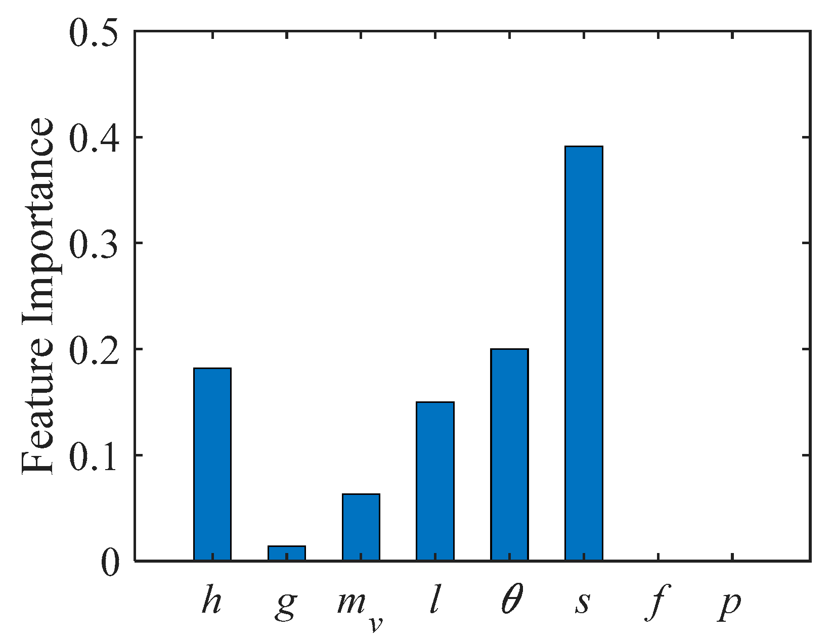
In this section, we will introduce the experimental setting, optimization results, ablation study, comparative experiment, and generalization ability of the proposed method.

4.1. Experimental Setting

To evaluate the performance of the proposed method, we conducted a series of experiments with the measured radar data. First, we discussed the effect of DNN structure on prediction performance. Second, the contribution of KPM and KWF were performed. Third, to verify the performance of the proposed method, we compared the predicted values with those estimated by other empirical methods or state-of-the-art machine learning (ML) methods. Finally, we also provide further experiments to evaluate the generalization capability of the proposed method.

It can be noted that the proposed method was mainly implemented with the Keras framework and end-to-end trained on Windows workstation with a GPU of Nvidia Tesla V100S. Furthermore, the learning rate during the training process is equal to 10 × 10⁻³. The batch size and epoch are set to 1024 and 100, respectively. Quantitatively, three common error indices were used to assess the prediction performance, namely the root mean square error (RMSE), Bias, and mean absolute percentage error (MAPE), with

$$\mathrm{R}\mathrm{M}\mathrm{S}\mathrm{E}=\sqrt{{\displaystyle \frac{1}{m}}{\displaystyle \sum _{i=1}^m{(p_i-y_i)}^2}}$$

(16)

$$\mathrm{B}\mathrm{i}\mathrm{a}\mathrm{s}={\displaystyle \frac{1}{m}}{\displaystyle \sum _{i=1}^m(p_i-y_i)}$$

(17)

$$\mathrm{M}\mathrm{APE}={\displaystyle \frac{100\%}{m}}{\displaystyle \sum _{i=1}^m\left|p_i-g_i\right|}$$

(18)

where $p_i$ and $y_i$ are the i-th predicted result and ground truth, respectively. m is the number of data points.

Before presenting the experimental results, it is worth mentioning at this point that we randomly selected 70% sets of the updated MFCD for training, 20% for validation, and the rest for testing. Furthermore, according to Equation (3), it can be observed that the input dimension is 8. Since principal component analysis (PCA) can reduce redundancy and stabilize training, we used PCA to decrease the dimension of the input variables, and the preserved principal components are equal to 6. Moreover, in order to minimize the biased predictions, all experiments were carried out with five independent tests, and the average values were reported for all the error indices.

4.2. Optimization of the Cascaded DNN Solver

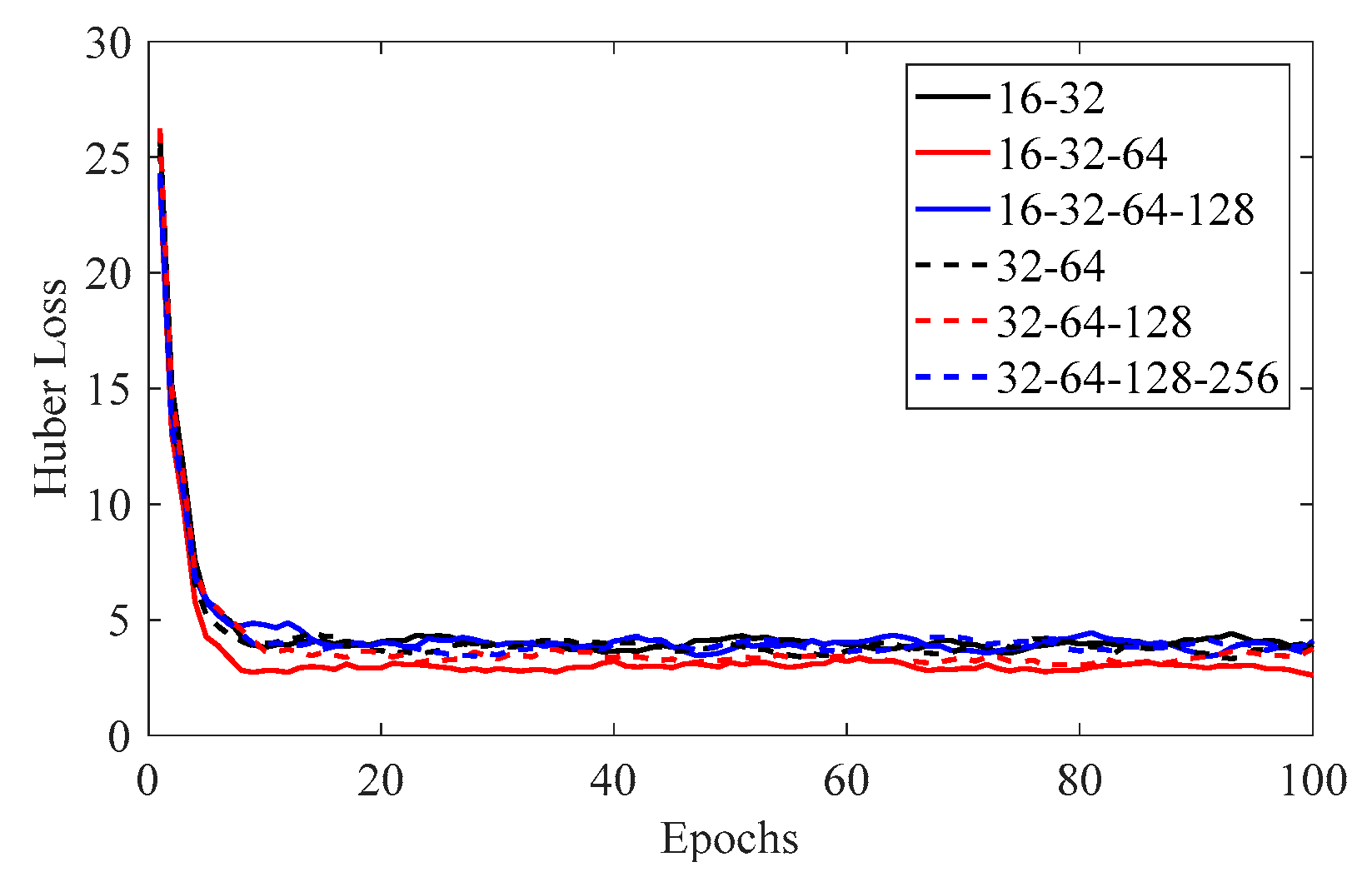
In order to improve the performance of the cascaded DNN solver and reduce the computational cost and time, a relatively optimal network structure must be performed before model training and prediction. Due to the excessive combinations of hidden layers and neurons, several alternatives are prepared in advance for convenience, i.e., 16-32, 16-32-64, 16-32-64-128, 32-64, 32-64-128, and 32-64-128-256, respectively. Note that, 16-32 denotes that the cascaded DNN solver is equipped with two hidden layers, and the neurons in each layer are 16 and 32, respectively.

Figure 5 shows the Huber loss of the above-mentioned cases. We can observe from Figure 5 that, in the case of 16-32-64, the proposed method achieves the minimum loss value during the training process, while the other configurations have slightly larger ones. Moreover, we also calculate the error indices on test dataset for different configurations, and the results are listed in

Table 4. Error indices for different DNN configurations.

Configurations	RMSE (dB)	Bias (dB)	MAPE (%)
16-32	5.06	0.72	12.9
16-32-64	4.48	0.91	10.6
16-32-64-128	5.04	1.03	13.3
32-64	4.78	0.42	11.4
32-64-128	4.75	0.34	11.2
32-64-128-256	4.80	0.52	11.2

. Similarly, it can be seen that the RMSE reaches the lowest value of 4.48 dB for the case of 16-32-64. When the cascaded DNN is configured with two or four hidden layers, the values of RMSE are slightly larger than those with three layers, e.g., the RMSEs of 16-32 and 16-32-64-128 are, respectively, 5.06 and 5.04 dB. This is because two hidden layers are not sufficient to adequately extract the features within the input, whereas four hidden layers achieve more redundant features, both of them reducing the model accuracy. Concerning the Bias, all configurations seem to overestimate the results of the test dataset. This may be explained by the fact that the complexity and variability of the surface features lead to a large dynamic range of radar echoes. Generally, MAPE represents the relative size of errors. From Table 4, it can be observed that, when the DNN solver employs the configuration of 16-32-64, the model achieves the best MAPE with the lowest value of 10.6%, demonstrating that the relative error is minimized under this configuration.

In summary, the above outcomes demonstrate that when the configuration of the cascaded DNN is 16-32-64, the proposed method achieves the best performance, and therefore, all the subsequent experiments were conducted on this configuration.

4.3. Ablation Study

To quantitatively validate the effectiveness of each key component in our proposed KADL framework, we conducted a comprehensive ablation study on the test dataset. The experiment was designed to systematically evaluate the contribution of the KPM and the KWF strategy by progressively adding them to a baseline model. Specifically, we combined the different components into four groups, namely,

(1)

Baseline: A standard DNN solver with three Dense layers (16-32-64 neurons) and ReLU activations, consistent with the structure illustrated in Section 4.2. This model processes the raw input features without KPM and KWF.

(2)

w/o KPM: The Baseline model enhanced with the KWF strategy but without the KPM. The KWF module processes the baseline features directly.

(3)

w/o KWF: The Baseline model enhanced with the KPM, but without the KWF strategy. The output of the KPM is directly fed to the final regression layer.

(4)

KADL: The complete proposed model incorporating both KPM and KWF components.

The quantitative results are shown in

Table 5. Quantitative results for different components in KADL.

	DNN	KPM	KWF	RMSE (dB)	Bias (dB)	MAPE (%)
Baseline	√	×	×	5.46	1.05	14.9
w/o KPM	√	×	√	5.18	0.93	13.6
w/o KWF	√	√	×	5.22	1.01	13.3
KADL	√	√	√	4.84	0.67	11.2

. We can make the following observations from Table 5. First, the Baseline achieves the worst performance, with the RMSE, Bias and MAPE reaching the values of 5.46 dB, 1.05 dB, and 14.9%, respectively. This indicates that while a powerful feature extraction method, pure data-driven DL model has inherent limitations in BC prediction tasks. Second, the results demonstrate both the KPM and KWF individually provide significant performance enhancements over the Baseline. Specifically, the model incorporating KWF (i.e., w/o KPM) show an obvious improvement, reducing the RMSE to 5.18 dB, and the MAPE to 13.6%. This observation confirms that KWF serves as an effective feature calibration mechanism. Similarly, w/o KWF also achieves a superior performance, with the RMSE of 5.22 dB, and MAPE of 13.3%, indicating its capability to capture meaningful representation from the input. Furthermore, an interesting phenomenon can also be observed that w/o KPM performs slightly better than w/o KWF, demonstrating that KWF contributes more significantly to the predictions. Third, the complete KADL model, which integrates both KPM and KWF, achieves the best performance across all metrics, with the RMSE of 4.84 dB, Bias of 0.67 dB, and MAPE of 11.2%. This result is not only better than the Baseline but also surpasses each ablated variant, proving that these two components are complementary.

In addition, we also evaluated the contribution of each component on different land covers, and the results are presented in

Table 6. Quantitative results of different land covers for different components in KADL.

Land Cover	RMSE (dB)				Bias (dB)				MAPE (%)
	Baseline	w/o KPM	w/o KWF	KADL	Baseline	w/o KPM	w/o KWF	KADL	Baseline	w/o KPM	w/o KWF	KADL
CL	5.53	5.18	5.24	4.93	0.94	0.76	0.34	0.51	14.7	13.1	13.3	11.2
Forest	5.77	5.11	5.13	4.89	1.02	0.96	0.78	0.85	15.2	14.2	14.1	13.3
GL	5.34	4.92	4.99	4.73	0.87	0.73	0.91	0.84	15.9	13.9	13.2	12.4
WB	4.76	4.42	4.58	4.13	0.92	0.97	1.05	0.93	13.6	12.3	12.0	11.5
AS	5.11	4.65	4.73	4.58	0.55	0.94	0.86	0.72	16.1	14.8	14.5	13.7

. In the first column of Table 6, CL denotes Cultivated Land, WB stands for Water Bodies, GL and AS represent Grass Land and Artificial Surfaces, respectively. It can be observed that the proposed KADL demonstrates the best overall performance, achieving the lowest RMSE values over these five land covers. In terms of Bias and MAPE, the proposed KADL also shows excellent performance. It obtains the lowest Bias for Forest, GL, and WB, and the lowest MAPE for all of these five land covers. Furthermore, the performance of the ablated models (i.e., w/o KPM, and w/o KWF) consistently lies between the Baseline and the KADL model for the vast majority of cases. This observation confirms that both the KPM and the KWF strategy provide significant improvements regardless of the land cover type, indicating the integration of the KPM and the KWF strategy offers decisive advantages for radar backscatter prediction in complex, heterogeneous environments.

4.4. Comparative Experiments

For comprehensive benchmarking and to better verify the proposed KADL, our experimental design leverages diverse representative methods categorized as, (a) the empirical-based methods, i.e., NTCM, and ANTCM, (b) machine learning-based regressors, i.e., random forest (RF), (c) the state-of-the-art DL model, i.e., DNN, 1D convolutional neural network (1D CNN), and 1D CNN with Transformer, denoted as 1DCNNT, and (d) the proposed KADL.

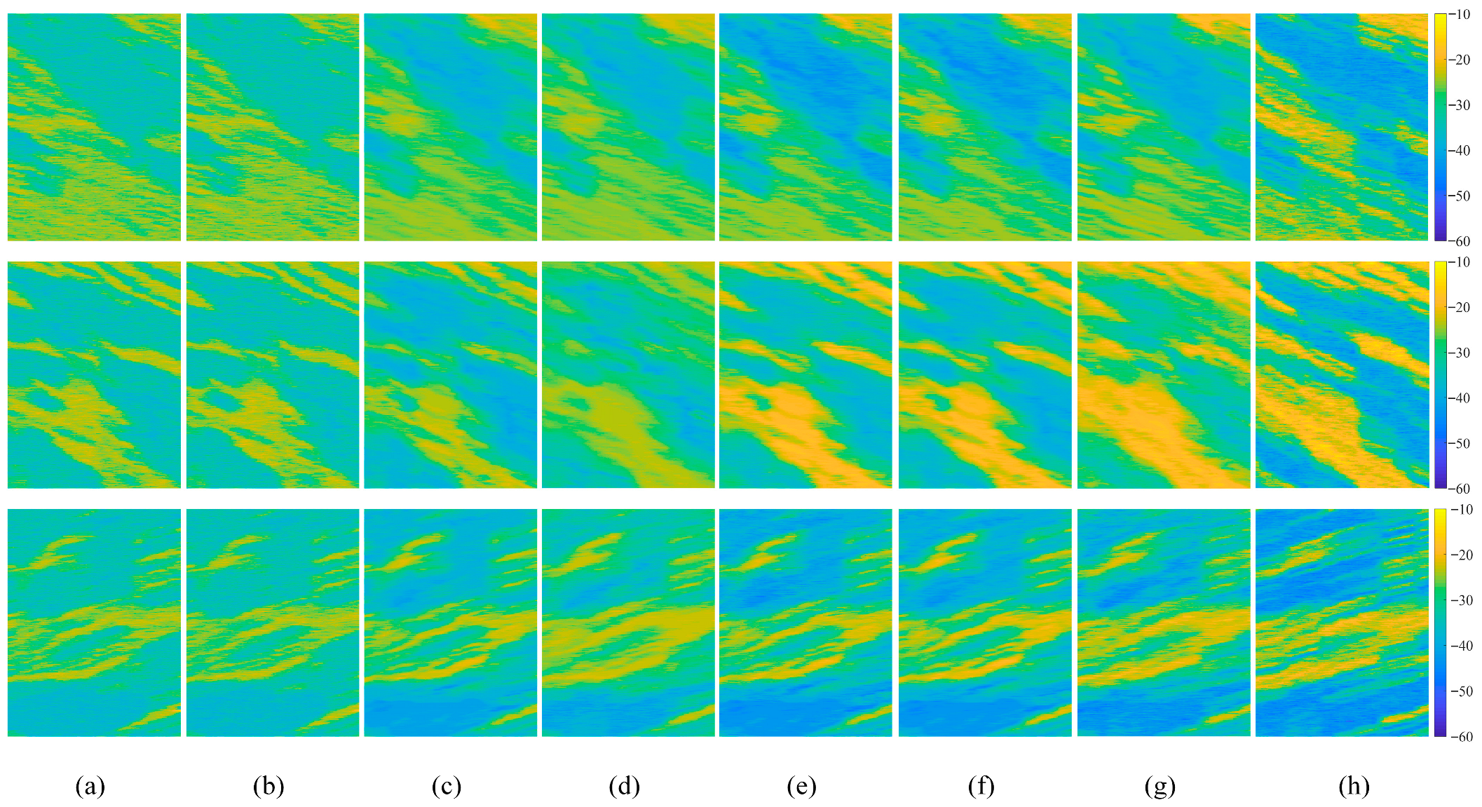
To intuitively visualize the predictions of the KADL method, we synthesized the predicted values as clutter maps based on the spatial coordinates of CCs. Typically, a clutter map provides absolute values of the BC for all CCs within the study area and represents the information on how the radar backscatter varies in the spatial domain. Figure 6 presents three samples (namely T1, T2, and T3) of the predicted results for different methods. It can be noted that these samples consist of 400 × 100 CCs, i.e., each CC represents a pixel and is denoted by a BC. In general, all these methods can reconstruct the discriminative features of the terrains. Specifically, the performance of NTCM, ANTCM, and DNN is slightly inferior to that of KADL, while RF, 1DCNN, and 1DCNNT achieve comparable results.

To quantitively estimate these observations, the error indices are computed and listed in

Table 7. Error indices of T1, T2, and T3 for different methods.

Methods	RMSE (dB)			Bias (dB)			MAPE (%)
	T1	T2	T3	T1	T2	T3	T1	T2	T3
NTCM	6.96	7.03	7.86	1.71	0.07	1.95	18.5	20.6	18.2
ANTCM	6.75	6.92	7.73	1.65	0.07	1.89	18.2	20.1	17.9
RF	5.19	5.35	5.80	0.80	0.11	1.71	13.6	14.8	13.6
DNN	5.42	5.70	6.11	2.11	0.87	1.81	14.0	16.5	13.0
1DCNN	5.08	5.26	5.60	1.68	0.12	1.41	12.7	14.7	11.9
1DCNNT	4.92	5.19	5.39	1.31	0.10	1.35	12.4	14.5	11.2
KADL	4.89	5.02	5.30	1.88	0.74	1.53	12.5	14.2	10.8

. From this table, it can be seen that, for all of these samples, empirical-based methods achieve the worst predicted results. For example, the RMSEs of NTCM and ANTCM for sample T3 reach the values of 7.86 dB, and 7.73 dB, respectively. Similarly, the MAPEs for this case reach the values of 18.2%, and 17.9%, respectively, which are higher than those of other methods. Compared to NTCM, although ANTCM exhibits some improvement in accuracy, their results still fall short of satisfactory levels, sufficiently demonstrating the limitations of traditional empirical-based models. Conversely, RF, 1DCNN, and 1DCNNT achieve a relatively better performance, compared to empirical-based methods. Regarding the RMSE, RF, 1DCNN, and 1DCNNT show considerable improvement for these three samples. Taking T1 as an example, the RMSE values of RF, 1DCNN, and 1DCNNT are 5.19 dB, 5.08 dB, and 4.92 dB, respectively, demonstrating the effectiveness of these intelligence algorithms. It also can be observed that, compared to RF and 1DCNN, 1DCNNT achieves slightly better results in terms of all these error indices, indicating the powerful feature extraction capabilities of transformers. As expected, KADL reliably surpasses the performance of all these comparative methods, including the standard DNN, the 1DCNN, and the more advanced 1DCNNT. This observation validates that the integration of KPM and KWF modules provides a distinct advantage over purely data-driven architectures. In addition, regarding the Bias, all these methods seem to overestimate the BC. This can be explained by the fact that the interaction between radar signal and land surface is highly complex, thus rendering the inadequate characterization by current models.

Table 8. Standard deviation of RMSE between five independent tests on T1, T2 and T3.

Methods	std-RMSE (dB)
	T1	T2	T3
NTCM	0.35	0.37	0.35
ANTCM	0.32	0.33	0.34
RF	0.30	0.31	0.30
DNN	0.31	0.29	0.32
1DCNN	0.29	0.23	0.30
1DCNNT	0.28	0.23	0.25
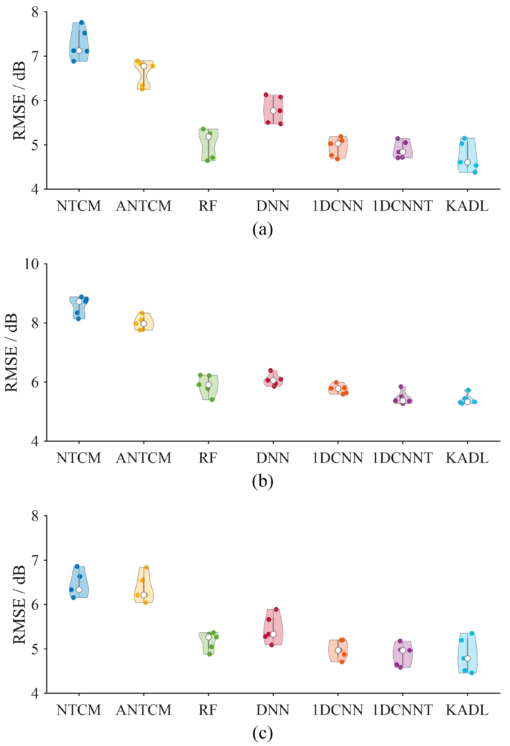
KADL	0.22	0.19	0.21

shows the standard deviation of the RMSE (std-RMSE) between five independent tests. Specifically, a lower std-RMSE indicates that the performance of models is more consistent and repeatable, while a higher std-RMSE suggests that the model is unstable and varies significantly from one trial to another, making its results less dependable. From Table 8, we can see that, the std-RMSE of KADL is substantially lower than that of the empirical models (NTCM, and ANTCM) and the traditional machine learning model (RF), achieving the values of 0.22 dB, 0.19 dB, and 0.21 dB, respectively. It also shows a clear improvement in stability over the other DL models (DNN, 1DCNN, and 1DCNNT). Furthermore, Figure 7 depicts the violin plots for RMSE distributions across five tests. It can be seen that KADL still exhibits strong robustness compared to other comparative methods, demonstrating its superiority.

The aforementioned results demonstrate that the proposed KADL perform better than empirical methods and ML methods in predicting BC from large areas, indicating the effectiveness of KADL. This is because KADL not only incorporates the effect of surface dielectric properties on radar backscatter, but also consistently focuses on the key features within the model construction.

4.5. Generalization Capability

A well-designed DL network requires not only a good accuracy on the test dataset, but also a good generalization to the new or unknown data. Therefore, we additionally registered the data of three areas (namely G1, G2, and G3) in the test region according to the method given in [35] to evaluate the generalization capability of the proposed KA method. It should be noted that the data from these areas were not involved in the model training process.

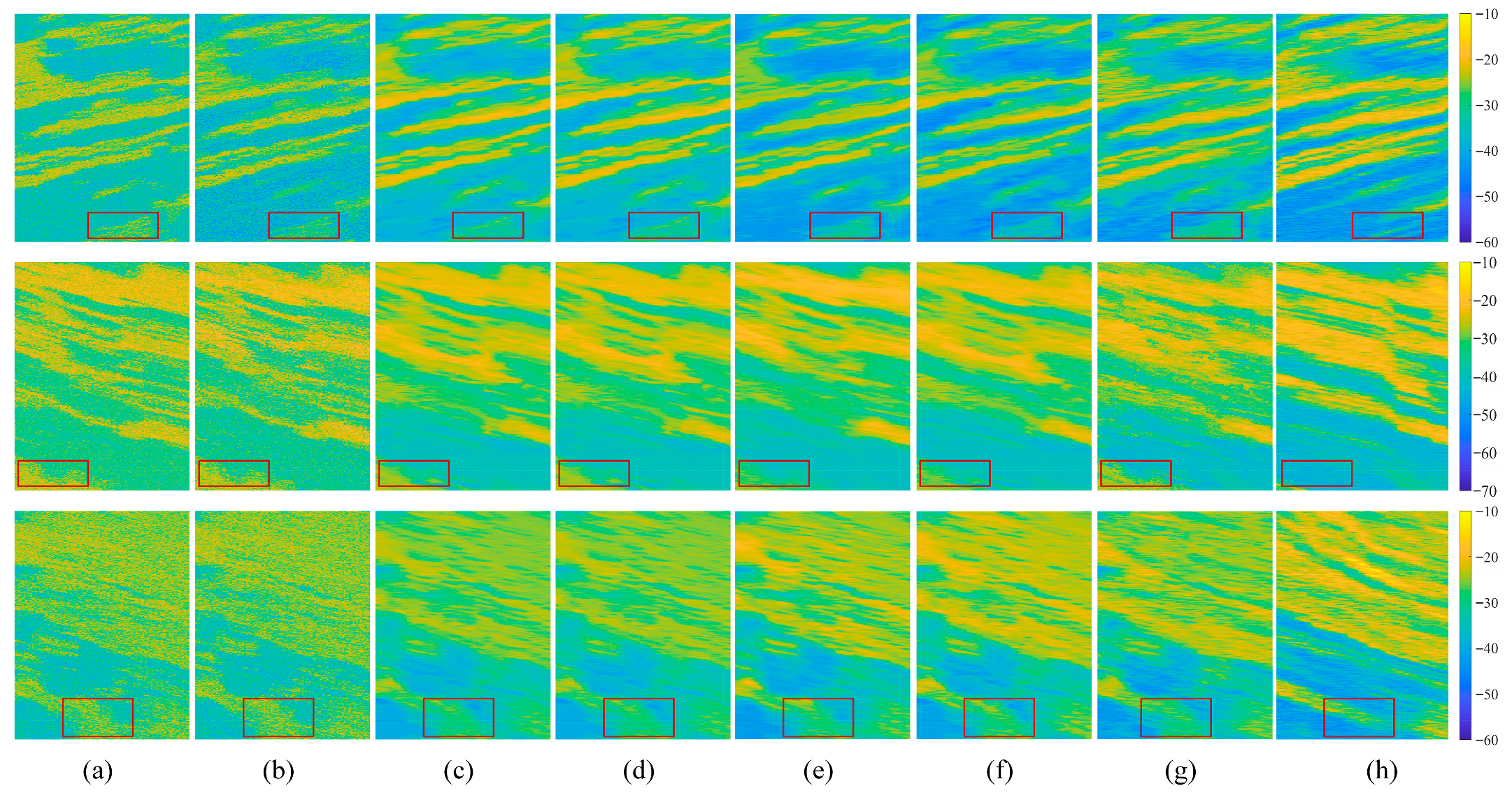
Figure 8 shows the clutter map of G1, G2, and G3 generated by different methods. In general, all these methods can reproduce the primary scattering characteristics of the study area. However, slight discrepancies can be observed visually between the predictions and the measured data in terms of amplitude. To quantitively estimate these differences, Table 8 lists the corresponding error indices. We can make the following observations from

Table 9. Error indices of G1, G2, and G3 for different methods.

Methods	RMSE (dB)			Bias (dB)			MAPE (%)
	G1	G2	G3	G1	G2	G3	G1	G2	G3
NTCM	7.28	8.58	6.46	1.92	2.27	0.83	17.9	21.7	17.6
ANTCM	6.62	7.99	6.37	1.57	1.39	0.66	11.5	17.1	15.5
RF	5.03	5.91	5.18	0.86	1.08	−0.19	12.4	14.5	14.8
DNN	5.79	6.07	5.45	2.64	2.56	0.18	10.6	11.4	13.2
1DCNN	4.95	5.76	4.99	0.72	0.95	0.11	12.5	13.3	14.3
1DCNNT	4.89	5.47	4.87	0.75	0.88	−0.23	11.4	12.4	13.9
KADL	4.74	5.42	4.86	1.84	1.89	−0.21	8.7	9.9	10.8

. First, empirical-based models, i.e., NTCM and ANTCM, yield the largest errors compared to other methods. For G2, they even obtain the RMSEs of 8.58 and 7.99 dB, proving the limitations of such models in real-world scenarios. Second, RF, and DNN give comparable predictions. More specifically, DNN performs somewhat behind, with higher RMSE values of 5.79 dB, 6.07 dB, and 5.45 dB for these three areas. Furthermore, 1DCNN and 1DCNNT obtain improved performance, with all the evaluation metrics better than RF and DNN. Third, with respect to Bias, almost all the models overestimate the measured BC. This occurrence presents further evidence of the intricate nonlinear relationship between radar signals and land features. Fourth, it is clear that the proposed KADL yields the best estimations, with the RMSE values of 4.74, 5.42, and 4.86 dB, respectively. This can be benefited from the fact that throughout the construction of KADL, KPM and KWF consistently focus on the contribution of key features to the BC, thus improving the generalization ability of the proposed method. Furthermore, regarding to the MAPE, KADL also yields the best results, with the values of 8.7%, 9.9%, and 10.8%, respectively.

Table 10. Standard deviation of RMSE between five independent tests on G1, G2 and G3.

Methods	std-RMSE (dB)
	G1	G2	G3
NTCM	0.35	0.33	0.34
ANTCM	0.33	0.32	0.32
RF	0.32	0.27	0.24
DNN	0.29	0.28	0.25
1DCNN	0.24	0.25	0.23
1DCNNT	0.22	0.21	0.20
KADL	0.19	0.21	0.18

presents the std-RMSE across these three samples. As can be seen in this table, the proposed KADL model demonstrates exceptional stability, achieving the lowest std-RMSE on both the G1 (0.19 dB) and G3 (0.18 dB) test samples. As for the G2, 1DCNNT obtains the comparable results, with the std-RMSE reaching the value of 0.21 dB. Figure 9 shows the violin plots for RMSE distributions, further demonstrating that the proposed KADL framework is not only more accurate but also significantly more robust and reliable than the benchmark models.

To further explore the robustness of the proposed method, we provide the boxplot for different methods, and the results are shown in Figure 9. In general, box plots indicate the dispersion of the reference data by means of statistical indicators. As can be seen in Figure 9, empirical-based methods are more sensitive to the outliers (i.e., red dotted line), with the largest differences acquired for all three areas. RF, DT, SVM and DNN obtain similar results, but both outperform NTCM and ANTCM. Furthermore, the proposed KADL achieves the best results and is more robust to outliers as expected (see Figure 9), indicating the superiority of KADL for estimating the BC for complex scenarios.

5. Discussion

5.1. Further Assessment of ANTCM

Although radar experiments remain the most direct approach for acquiring land backscatter data and analyzing its characteristics, exhaustive measurements covering all potential radar configurations incur operationally prohibitive temporal and resource investments. As part of this work, ANTCM serves as an alternative for BC estimation where KA or data-driven solutions prove infeasible. While exhibiting more cost-effective than data-driven DL method in backscatter research, the foundational architecture of ANTCM relies on established empirical models to simulate land cover-specific BC. Crucially, this method maintains long-term viability through its modular design, enabling systematic updates to radar backscatter modeling components as radar technological advancements emerge.

5.2. Further Assessment of KADL

As evidenced by the comparative analysis in the above-mentioned results, the proposed KADL successfully preserves critical topographic signatures across heterogeneous terrain regions, demonstrating robust feature retention capabilities. On the one hand, we additionally took into account the effect of surface dielectric characteristics on BC by introducing soil moisture and LAI in MFCD. KADL is designed to alleviate the limitations of empirical models by constructing a nonlinear mapping relationship between multidimensional parameters and BC. On the other hand, the proposed KPM and KWF enable the KADL to focus on discriminative features throughout the whole prediction process, thus boosting the accuracy. In practice, with access to representative parameters of the region of interest, one can obtain the distribution of the BC according to radar parameters, thus providing a novel insight into the investigation of radar backscatter in complex or unknown areas.

However, a well-constructed dataset is critical for enabling models to handle real-world variations and enhance robustness across diverse operational scenarios. The generalization capability of the proposed KADL framework is inherently tied to the precision of its registered input data. Therefore, we would like to make a few additional comments on the shortcomings of KADL. Typically, feature importance is an assessment of the influence of features on the predictive effectiveness for the model. Figure 10 illustrates the importance of different features according to RF, and the results reveal that geometric parameters dominate BC predictions, i.e., elevation h, grazing angle θ, and shadowing proportion s. Specifically, shadowing proportion s (importance score ≈ 0.4) exerts the strongest influence, followed by grazing angle and elevation. This geometric dependence is visually corroborated in Figure 8 and Figure 11, where three representative regions in G1, G2, and G3 are analyzed with red rectangular markers for cross-comparison. Taking G2 as an example, the ground-truth BC shown in Figure 8h exhibit spatially smooth gradients, whereas KADL and other methods shown in Figure 8a–g display non-uniform fluctuations. These discrepancies align with geometric parameter trends in Figure 11. Concretely, while elevation and grazing angle vary gradually, shadowing proportion shows abrupt transitions. These observations demonstrate that the performance of the proposed model is highly sensitive to the accuracy of shadowing judgment algorithms. Therefore, integrating high-resolution DEMs and advanced shadow estimation algorithms to improve prediction accuracy is a question worth considering.

6. Conclusions

This article proposes a novel KADL method to overcome the limitation of empirical models in predicting radar backscatter for large-scale heterogeneous scenarios. Firstly, based on multi-source remote sensing data, we incorporated the dielectric properties of the land surface into MFCD, and obtained the initialized input parameters. Secondly, a cascaded DNN solver coupled with a well-designed KPM was used to better capture the representative features within the inputs. Thirdly, a KWF strategy was introduced to force the network to pay more attention on the key features, while suppressing redundant ones, improving the accuracy for backscatter prediction. Extensive experiments conducted on airborne radar measurements reveal that the proposed KADL outperforms the traditional empirical models and state-of-the-art methods, in terms of accuracy, robustness, and generalization ability. This novel idea will serve as a new path for further investigation of radar backscatter from large-scale heterogeneous scenarios.

However, our work still has limitations, (1) as state in Table 8, the test site contains only five terrain features, and the radar configurations are also limited, and (2) the predicted results of KADL depend on the reliability of the shadowing estimation algorithm. In the future, experiments should be undertaken over more feature types and radar configurations to broaden the applicability of KADL method. On the other hand, we will actively explore more accurate shadow discrimination methods.