Self-Supervised Learning for Soybean Disease Detection Using UAV Hyperspectral Imagery

Highlights

What are the main findings?

• A self-supervised learning framework achieves 92% accuracy in early soybean disease detection using unlabelled UAV hyperspectral data, matching supervised baselines.
• A distance-based spectral pairing technique enables effective feature learning directly from canopy reflectance without manual annotations.

What are the implications of the main findings?

• The framework addresses the annotation bottleneck in remote sensing, enabling scalable early disease detection for large-scale agricultural monitoring.
• The approach reduces reliance on expert-labeled field data while maintaining high accuracy, making precision agriculture more accessible and cost-effective.

Abstract

The accuracy of machine learning models in plant disease detection significantly relies on large volumes of knowledge-based labeled data; the acquisition of annotation remains a significant bottleneck in domain-specific research such as plant disease detection. While unsupervised learning alleviates the need for labeled data, its effectiveness is constrained by the intrinsic separability of feature clusters. These limitations underscore the need for approaches that enable supervised early disease detection without extensive annotation. To this end, we propose a self-supervised learning (SSL) framework for the early detection of soybean’s sudden death syndrome (SDS) using hyperspectral data acquired from an unmanned aerial vehicle (UAV). The methodology employs a novel distance-based spectral pairing technique that derives intermediate labels directly from the data. In addition, we introduce an adapted contrastive loss function designed to improve cluster separability and reinforce discriminative feature learning. The proposed approach yields an 11% accuracy gain over agglomerative hierarchical clustering and attains both classification accuracy and F1 score of 0.92, matching supervised baselines. Reflectance frequency analysis further demonstrates robustness to label noise, highlighting its suitability in label-scarce settings.

1. Introduction

Extreme climate events have intensified plant disease outbreaks over the past two decades, driven by rising temperatures, altered precipitation regimes, and humidity fluctuations [1,2,3]. Soybeans, a globally important crop for protein and oil, are particularly vulnerable to climate-driven stresses, with heightened disease susceptibility threatening yield stability and long-term food security [4,5]. Conventional visual inspection remains the primary diagnostic method, but is labor-intensive, subjective, and inadequate for early detection when timely intervention is most critical [6]. Advances in remote sensing, integrated with machine learning, now offer scalable, non-invasive monitoring solutions that enable earlier diagnosis, targeted pesticide application, and potential yield improvements, while reducing environmental impacts [7]. However, these approaches predominantly rely on supervised learning frameworks that require large volumes of manually annotated training data.

Recent work on plant disease detection has largely centered on leaf-image analysis with computer vision. Convolutional neural networks (CNNs) achieve high accuracy in controlled settings, predominantly on leaf image datasets [8]. However, leaf-image methods are poorly suited for identifying diseases before visible symptoms emerge, as many stressors do not manifest visibly on the leaf surface [9], and image acquisition at scale is operationally burdensome for commercial agriculture. This limitation extends to self-supervised learning approaches, which have primarily focused on controlled leaf-image datasets [10,11] rather than field-scale canopy monitoring.

To overcome these spatial and operational limitations of leaf-level approaches, unmanned aerial vehicles (UAVs) with hyperspectral sensors offer a field-scale alternative and have shown promise for early disease detection in experimental and commercial settings [12,13]. Narrow bands in the red-edge and near-infrared regions are sensitive to water status and subtle physiological changes that precede visible symptoms [14]. Despite these potential, the practical deployment of UAV-based hyperspectral imaging for early detection faces a critical bottleneck, as most supervised pipelines require large volumes of expertly labeled, in situ data [15,16]. This dependency is especially problematic when symptoms are pre-visual and subtle, making annotation time-consuming, costly, and subjective [17,18]. The challenge is amplified for root-origin diseases such as soybean sudden death syndrome (SDS), where early canopy signals are minimal and demand specialized expertise to identify reliably [19]. As a result, assembling sufficiently large labeled datasets for robust supervised learning remains prohibitively expensive for large-scale monitoring, underscoring the need for methods that reduce annotation burden while preserving accuracy.

Self-supervised learning (SSL) offers a methodology with particular promise for addressing scenarios characterized by limited labeled data. Unlike unsupervised learning, which is hindered by the curse of dimensionality and limited feature separability [20,21,22], SSL creates pseudo-labels through pretext tasks. This approach enables representation learning without extensive manual annotation while maintaining discriminative power. Recent SSL frameworks, including contrastive learning [23], Siamese networks [24,25], BYOL [26], and SimSiam [27], have demonstrated strong capabilities in extracting meaningful features from unlabeled data [28,29].

Despite SSL’s proven effectiveness in agricultural applications such as crop type classification and leaf-based disease detection [30], its potential for large-scale UAV-based hyperspectral monitoring of early-stage field diseases remains untapped. This gap is particularly critical because existing SSL frameworks face three key limitations when applied to field-scale monitoring. First, most existing studies focus on controlled leaf-image datasets [10,11], which are inadequate for detecting early-stage diseases like SDS, where symptoms manifest subtly at the canopy level before becoming visible on individual leaves. Second, SSL architectures designed for spatial features (typically CNN-based) do not directly transfer to hyperspectral data, which require specialized handling of high-dimensional spectral signatures [11,30,31]. Third, there is a lack of SSL frameworks specifically designed to leverage the unique characteristics of hyperspectral reflectance data, such as physiologically meaningful spectral bands in the red-edge and NIR regions, for early disease detection at the plot or field scale.

To address this critical gap, this study proposes a self-supervised learning framework for sudden death syndrome (SDS) detection in soybeans. The framework operates on canopy-level hyperspectral reflectance data acquired from unmanned aerial vehicles, enabling effective disease monitoring under label-scarce conditions. Unlike conventional approaches that depend on extensive manual annotation, particularly problematic for early-symptomatic diseases, our framework derives supervision signals directly from the intrinsic structure of unlabeled spectral data. The main contributions of this work are summarized as follows:

• An end-to-end self-supervised learning model is developed, specifically tailored for early-stage SDS detection using UAV hyperspectral data.
• A Euclidean distance-based pseudo-labeling strategy is introduced that leverages the physiologically meaningful separability in hyperspectral space to create high-confidence training pairs, enabling encoder training directly from spectral representations without manual annotation.
• A comparative evaluation is conducted to benchmark the SSL framework against conventional clustering algorithms and supervised classifiers.

This framework demonstrates that self-supervised learning can achieve performance comparable to supervised baselines while substantially reducing the reliance on labeled data, suggesting its potential as a scalable approach for hyperspectral-based plant disease detection in scenarios where manual annotation is limited or costly.

2. Materials and Methods

2.1. Study Area

The experimental site was situated in Montgomery County, Illinois, USA. The region experiences a continental climate, characterized by warm, humid summers and cold winters. According to data from the National Oceanic and Atmospheric Administration (NOAA), July is the warmest month, with an average temperature of 23 °C, while November is the coldest, averaging 6 °C. Rainfall peaks in May and gradually declines through November. The trials were conducted on Mollisol soils with a loam texture, commencing in May 2022. Experimental plots varied in size, ranging from 1.5 to 3 m in width and 5.5 to 6 m in length, with a row spacing of 0.76 m. Standard tillage practices were followed, and all trials were conducted under rainfed conditions. Disease symptoms emerged naturally and were in their early stages at the time of data collection in mid-August 2022. Harvesting occurred in October and November, in accordance with genotype maturity groups. Visual assessment of disease severity was conducted to confirm the disease status.

Disease status was determined through labor-intensive field assessment conducted on 15 August 2022, by pathological and phenological specialists from GDM Seeds. Evaluators independently inspected individual plots, examining stems and leaves for SDS symptoms, and the assessments were later compiled to establish final classifications. Following a conservative protocol, plots exhibiting yellowing, chlorosis, or damage on any observed stem or leaf were labeled as SDS-affected, while plots with no visible symptoms were labeled as healthy, a threshold that necessarily introduced some classification ambiguity in borderline cases with minimal symptom expression. 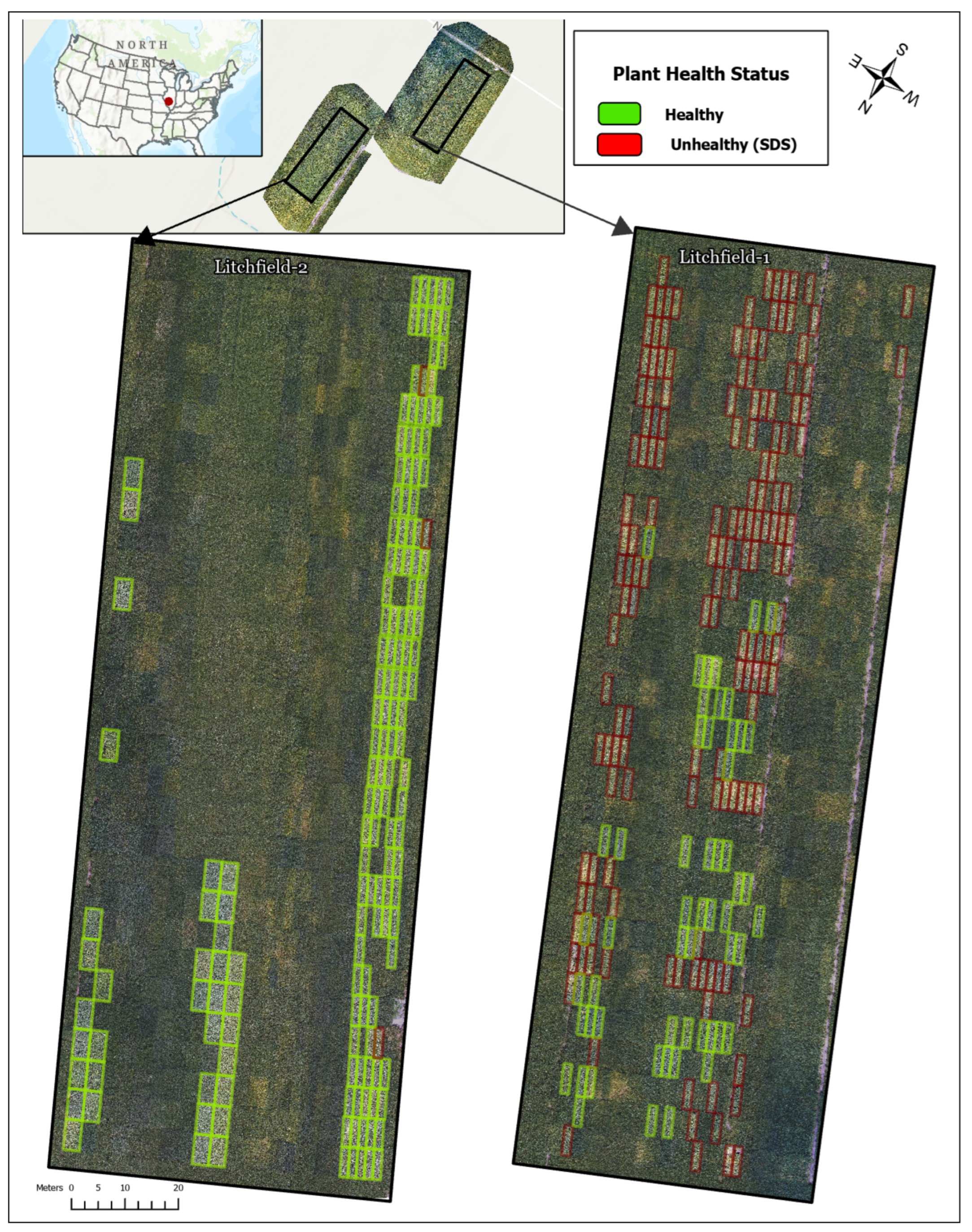Figure 1 provides an overview of the study area and plot layout of the 375 total plots, 206 were classified as healthy (55%) and 169 as SDS-affected (45%), representing a moderate class imbalance that was addressed during SSL training through balanced pair generation (Section 2.6). At this midpoint of the season, the plants were in the early to mid stages of their life cycle, and SDS was in an early development phase.

2.2. Materials

Hyperspectral data acquisition was conducted through a single field campaign in mid-August 2022 using a Headwall Nano-Hyperspec VNIR sensor (Headwall Photonics, Bolton, MA, USA) (400–1000 nm, 269 bands) mounted on a Matrice 600 Pro UAV (DJI, Shenzhen, China). The flight was executed at an altitude of 100 m above ground level, yielding a spatial resolution of approximately 4 cm per pixel. Georeferencing was performed using a mobile R12 Real-Time Kinematic (RTK) GNSS receiver (Trimble, Sunnyvale, CA, USA), which provided sub-centimeter-level positioning accuracy for ground control points. Raw hyperspectral data, initially distorted and non-georeferenced, were calibrated to consistent reflectance values for analysis. The dataset was split into training (80%, n = 300) and testing (20%, n = 75) sets using stratified sampling to maintain class distribution. The self-supervised learning framework was implemented in Python 3.10 using PyTorch 1.12, with data preprocessing and clustering analyses conducted using scikit-learn, NumPy, and pandas libraries.

2.3. Data Pre-Processing

The preprocessing pipeline transforms raw hyperspectral imagery into plot-level spectral signatures suitable for SSL training. Traditional SSL architectures predominantly employ CNNs, which necessitate extensive datasets, substantial computational resources, and rich spatial features to achieve effective feature separation [32,33,34]. However, the high dimensionality of HSI data and inadequate spatial features in early-stage crop vegetation increase architectural complexity [35]. To mitigate these challenges, this study utilizes plot-level mean spectra as the dataset, enhancing computational efficiency while preserving discriminative spectral information.

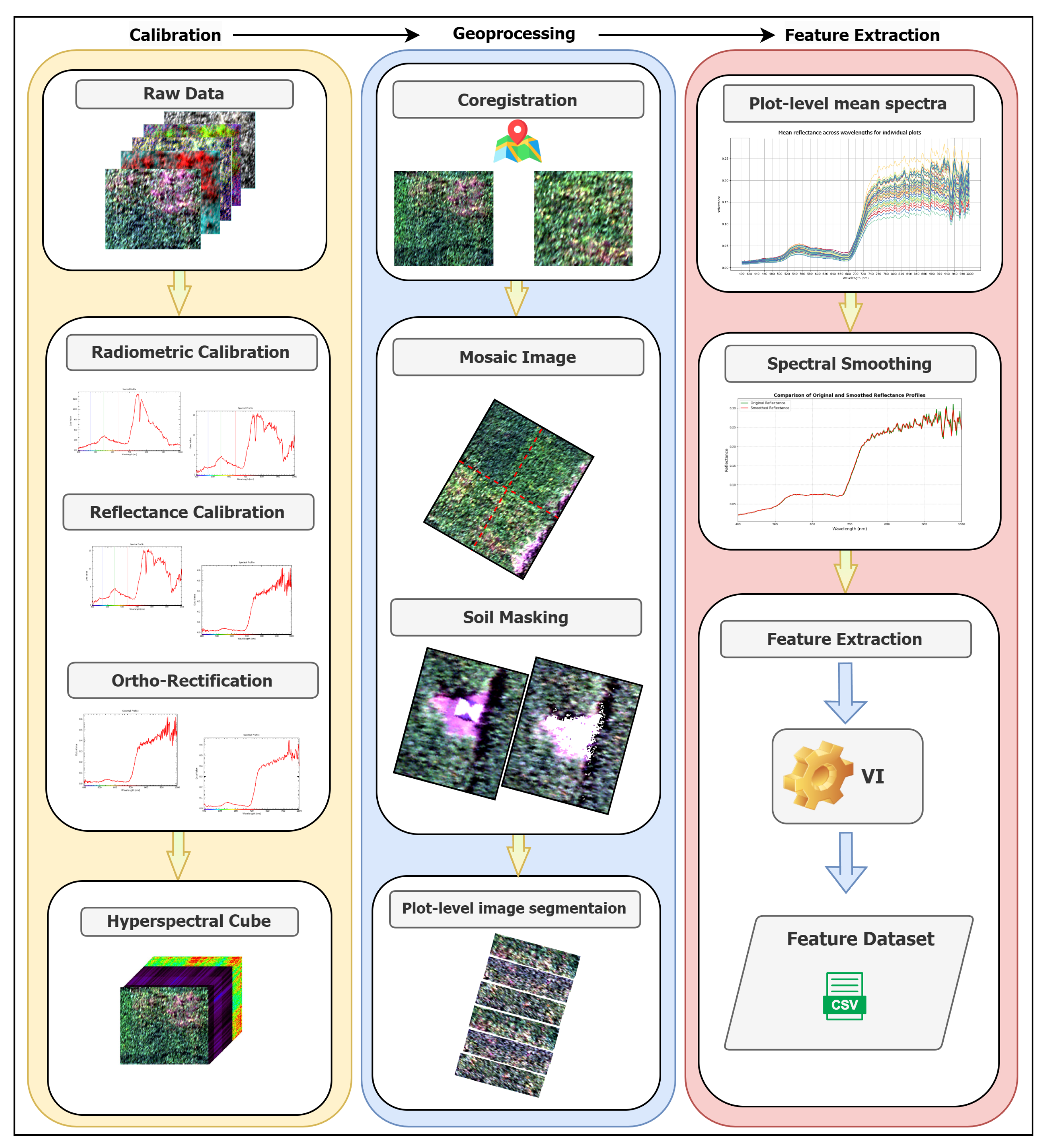
The preprocessing pipeline, illustrated in Figure 2, consists of three main stages. First, raw hyperspectral data undergo radiometric calibration to correct sensor-specific errors and convert digital numbers to standard reflectance values, followed by ortho-rectification to remove geometric distortions. Second, individual hyperspectral image cubes are georeferenced using the R12 RTK GNSS data and mosaicked to generate a seamless field-scale image.

Third, background soil and shadow pixels were removed using an adapted data-driven approach [36] to isolate pure canopy spectral signals. The soil masking technique exploits inherent spectral differences between vegetation and soil across VNIR wavelengths, using rule-based classification that leverages characteristic reflectance patterns of photosynthetically active vegetation versus bare soil. This unsupervised approach eliminates the need for manual training sample generation while maintaining robust performance. Shadow masking was implemented to detect and exclude shaded regions cast by the UAV platform and environmental conditions, ensuring spectral consistency across plots. Shadow removal is critical because shaded areas exhibit incomplete spectral information and reduced intensity values that could confound disease detection.

Following soil and shadow removal, plot-level mean reflectance signatures were computed exclusively from pure canopy pixels, ensuring that extracted spectral features represent genuine vegetation characteristics rather than mixed soil-plant or illumination artifacts. All spectra are then smoothed using the Savitzky-Golay filter to reduce noise. Subsequently, 47 vegetation indices spanning chlorophyll content ($NDVI, GNDVI, MCARI$ variants), water stress ($WBI, WSCT, NDWI$), pigment composition ($SRPI, NPCI, AR{I}_2$), and structural characteristics ($SAVI, OSAVI, MSAVI$) are computed from the 269 spectral bands using established formulas from the remote sensing literature (Table S2). These indices provide biophysically interpretable features that complement raw spectral signatures by encoding domain knowledge about vegetation stress responses. The 269 spectral bands and 47 derived indices are concatenated to form a 316-dimensional feature vector per plot, which undergoes standardization before model training.

2.4. Plot-Level Mean Spectra Analysis

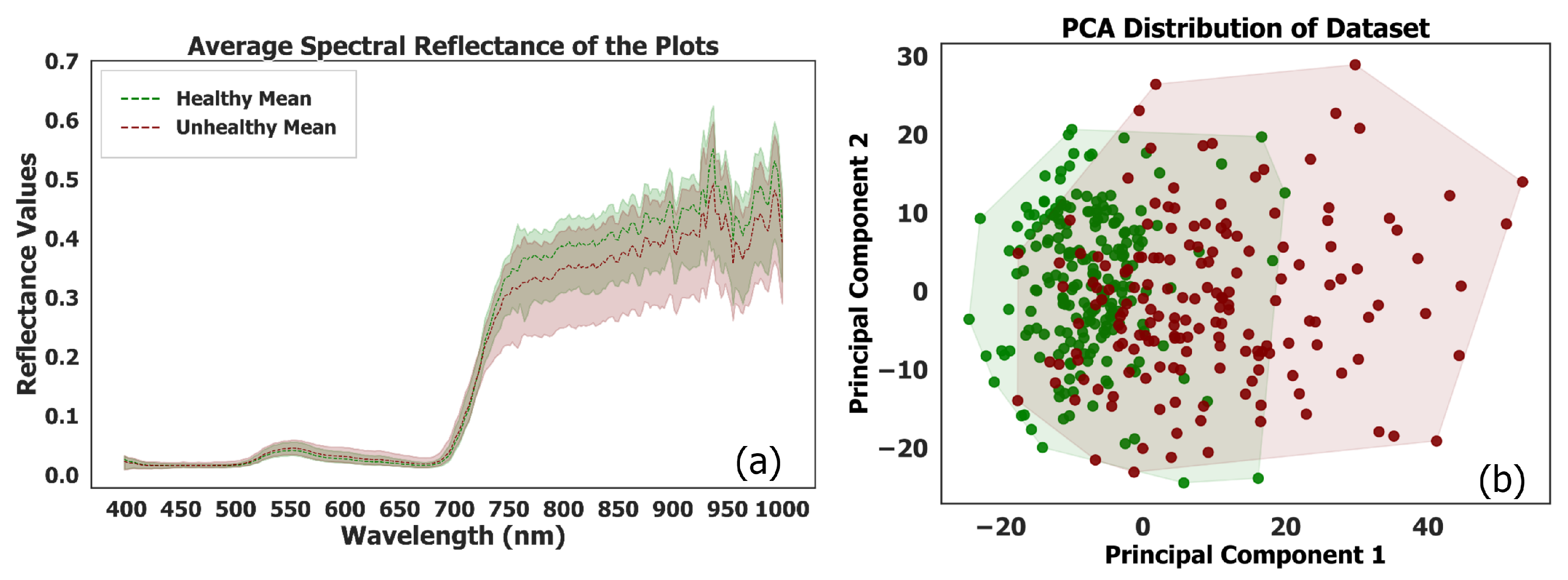
Despite rigorous filtering and calibration processes that maintain standard procedural integrity, notable edge noise persists within the dataset. Figure 3a illustrates the mean spectral reflectance curves for healthy and unhealthy plots. The spectral reflectance curves for unhealthy plots exhibit a broader horizontal distribution compared to those of healthy plots. This wider dispersion in spectral reflectance values indicates greater variability among unhealthy plots. Consequently, this variability complicates the differentiation between healthy and unhealthy plots when relying solely on spectral information. The increased spectral overlap highlights the challenge of using spectral data alone to accurately classify plot health, underscoring the need for incorporating advanced modeling techniques to enhance classification accuracy.

2.5. SSL Architecture

This section presents the self-supervised learning framework developed for SDS detection. As introduced in Section 1, we develop an SSL framework tailored to plot-level hyperspectral reflectance. Unlike methods predicated on spatial context (CNNs) or semantic tokenization (LLMs), our approach operates directly on tabular spectra, where neither assumption holds. The framework comprises: (i) a Siamese encoder architecture (Section 2.5), (ii) a spectral distance-guided pairing scheme that yields high-confidence positive/negative pairs from unlabeled data (Section 2.6), and (iii) an exponentiated contrastive loss that modulates the strength of inter/intra-class separation via a hyperparameter exponent (Section 2.7).

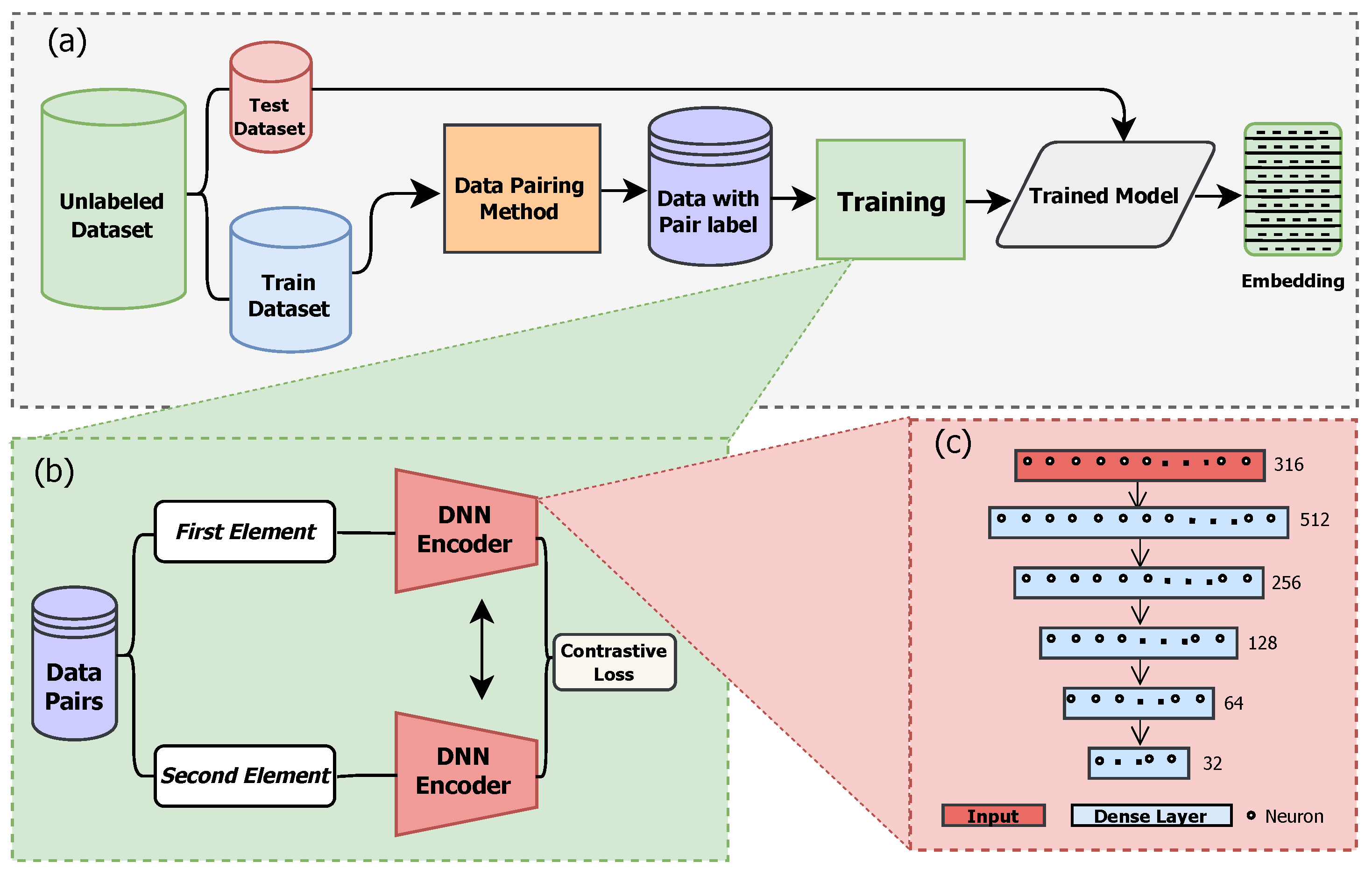
Figure 4 summarizes the training pipeline. Given an unlabeled dataset of per-plot index-reflectance vectors, we (a) standardize per band and construct pairs using the distance-guided data pairing method, (b) optimize a Siamese encoder with an exponentiated margin-based contrastive objective, and  (c) deploy the trained encoder to obtain low-dimensional embeddings for evaluation. For the encoder, we use a fully connected feed-forward network with five hidden layers, comprising 316 input neurons, successive layers of 512, 256, 128, and 64 neurons, and a 32-dimensional embedding output (ReLU activations and layer normalization). The 32-D embedding provides a compact representation sufficient for downstream separability while mitigating overfitting under limited labels. Training uses Adam (learning rate ${10}^{-3}$), $L_2$ regularization, early stopping (patience 25), and 300 epochs. Model training convergence under 30 min. After convergence, the encoder processes the test set to produce test-embeddings.

2.6. Distance-Based Pairing Strategy

We construct training pairs directly in standardized reflectance vectors, following distance-based SSL pretext (e.g., SimCLR [29], MoCo [37]). Let $X={\left\{x_i\right\}}_{i=1}^N\subset {\mathbb{R}}^B$ denoted normalized vi-spectra with B = 316. For uniformly sampled index pairs $(i, j)$, we compute Euclidean distance $d_{ij}={\parallel x_i-x_j\parallel }_2$ and assign high-confidence pseudo-labels using two thresholds $(\alpha , \beta )$ with $0<\alpha <\beta$:

$$\begin{array}{c}\left(P, L_S\right)=\bigcup _{k=1}^n\left\{\begin{array}{cc}((x_i, x_j), 0)\hfill & \mathrm{if}0 < \parallel x_i-x_j\parallel \le \alpha ,\hfill \\ ((x_i, x_j), 1)\hfill & \mathrm{if}\parallel x_i-x_j\parallel \ge \beta ,\hfill \end{array}\right.\\ \mathrm{where}0 \le \alpha \le \beta \mathrm{and}i\ne j\end{array}$$

(1)

Pairs with $\alpha < d_{ij} < \beta$ are discarded to avoid ambiguous supervision. Index pairs are de-duplicated, and similar/dissimilar counts are balanced to reduce label bias. Threshold selection in SSL poses an intrinsic challenge: appropriate cutoffs must be inferred from unlabeled data structure alone, precluding direct reliance on ground-truth validation.

A distribution-driven approach was adopted wherein thresholds are derived from empirical quantiles of the pairwise distance distribution. Distances were computed for a representative subset of training instances, with $\alpha$ and $\beta$ positioned at the 20th and 80th percentiles, respectively, yielding $\alpha =0.74$ and $\beta =1.51$ (Figure S1) in standardized spectral space. A total of 3000 pairs were generated ($n=3000$, with $n_{\mathrm{similar}}\approx n_{\mathrm{dissimilar}}$) with balanced distribution between similar and dissimilar labels to prevent class bias during training. This percentile-based threshold selection constitutes a data-adaptive strategy that instinctively scales to the intrinsic geometry of the feature space, obviating the need for manual tuning on labeled validation data, which would violate the self-supervised paradigm.

The 20th/80th percentile positions reflect a principled trade-off between pseudo-label confidence and training sample sufficiency: more conservative thresholds (e.g., 10th/90th percentiles) would yield higher-purity pairs at the cost of insufficient training diversity, while more permissive cutoffs (e.g., 30th/70th percentiles) would increase label noise in the contrastive signal. The adopted quartile-based approach ensures that approximately 40% of candidate pairs receive confident pseudo-labels (20% similar, 20% dissimilar), while the ambiguous middle 60% are excluded—a conservative strategy aligned with established self-supervised learning practices that prioritize signal quality over quantity. Crucially, this method generalizes across datasets because percentiles adapt to the observed distance distribution: a dataset exhibiting tighter spectral clustering would produce smaller absolute threshold values, while one with greater inter-class dispersion would yield larger thresholds, yet both would achieve equivalent relative separation in their respective feature spaces.

This adaptive property ensures methodological transferability without requiring dataset-specific hyperparameter tuning. This pairing strategy mitigates the class imbalance present in the raw dataset (55% healthy, 45% SDS-affected) by ensuring equal representation of both relationship types during contrastive learning. The quartile-based thresholds strike a balance between the need for sufficient training pairs and the requirement for high-confidence pseudo-labels, accepting approximately one-fifth of pairs as similar, one-fifth as dissimilar, and rejecting three-fifths as ambiguous. Algorithm 1 operationalizes this strategy with stratified sampling, gray-zone exclusion, de-duplication, and class balancing. The distance distribution exhibits (Figure S1) a unimodal structure with an extended right tail, characteristic of high-dimensional spectral data, where most pairs show moderate dissimilarity, with distributional extrema representing unambiguous cases. Euclidean distance on normalized vi-spectra preserves physiologically informative amplitude differences (red-edge, NIR regions), constitutes a proper metric for margin-based objectives, and enables computationally efficient pair generation.

Algorithm 1 Distance-Based Pair Generation

1: Initialize $S\leftarrow \varnothing$, $P\leftarrow \left[\right]$, $y\leftarrow \left[\right]$   2: Set $n_{\mathrm{similar}}, n_{\mathrm{dissimilar}}\leftarrow \lfloor n/2\rfloor$   3: Set $I\leftarrow \mathrm{indices}\left(X\right)$   4: while$\left|P\right|<n$do   5:    Randomly sample $i, j\in I$ where $i\ne j$   6:    $K\leftarrow \mathrm{sorted}\left(\right\{i, j\left\}\right)$ {Create unique pair identifier}   7:    if $K\notin S$ then   8:        Compute $d_{ij}={\parallel x_i-x_j\parallel }_2$   9:        if $d_{ij}\le \alpha$and$n_{\mathrm{similar}}>0$  then 10:            $P\leftarrow P\cup \left\{(x_i, x_j)\right\}$, $y\leftarrow y\cup \left\{0\right\}$ 11:            $n_{\mathrm{similar}}\leftarrow n_{\mathrm{similar}}-1$ 12:            $S\leftarrow S\cup \left\{K\right\}$ 13:        else if$d_{ij}\ge \beta$and$n_{\mathrm{dissimilar}}>0$ then 14:            $P\leftarrow P\cup \left\{(x_i, x_j)\right\}$, $y\leftarrow y\cup \left\{1\right\}$ 15:            $n_{\mathrm{dissimilar}}\leftarrow n_{\mathrm{dissimilar}}-1$ 16:            $S\leftarrow S\cup \left\{K\right\}$ 17:        end if 18:     end if 19: end while 20: return $P,y$

2.7. Contrastive Loss

The contrastive loss function trains the model using negative sampling to distinguish between similar and dissimilar pairs. We introduce a flexible exponential parameter n on top of the traditional contrastive loss to enhance model performance. This enhancement allows for better discrimination between similar and dissimilar pairs. The loss function $L(W, (Y, x_1, x_2))$ is defined as:

$$\begin{array}{c}\hfill \left(W, \left(Y, x_1, x_2\right)\right)={\displaystyle \frac{1}{N}}\sum _{i=1}^N{[\left(1-Y_i\right)·\parallel x_{1_i}-x_{2_i}\parallel }^n+Y_i·max\left(0, \mathrm{margin}-\parallel x_{1_i}-x_{2_i}{\parallel }^n\right)]\end{array}$$

(2)

Here, $x_{1_i}$ and $x_{2_i}$ represent the i-th pair of embedding vectors, and $Y_i$ is the corresponding label indicating whether the pair is similar $(Y_i=0)$ or dissimilar $(Y_i=1)$. The term $\parallel x_{1_i}-x_{2_i}\parallel$ denotes the Euclidean distance between the embeddings. For similar pairs $(Y_i=0)$, the loss is $\parallel x_{1_i}-x_{2_i}{\parallel }^n$, encouraging the embeddings to be close. For dissimilar pairs $(Y_i=1)$, the loss is $max{(0, \mathrm{margin} - \parallel x_{1_i}-x_{2_i}\parallel }^n)$, encouraging a distance greater than the margin. The overall loss is averaged over the total number of pairs N.

The traditional contrastive loss uses a fixed exponent of $n=2$, which limits the model’s ability to emphasize larger distances. By allowing n to vary, the modified loss can place greater emphasis on larger distances, resulting in better separation of dissimilar pairs in the embedding space. This flexibility leads to improved performance as the model becomes more sensitive to the nuances of the data. The optimal value of n for hyperspectral disease detection was determined through systematic ablation analysis (Section 2.8).

2.8. Evaluation Metrics

The embedding vectors generated from the trained model (Figure 4) encode feature representations for each data point. To evaluate the effectiveness of SSL, both the original and embedded test data are clustered using K-Means [38] and Agglomerative Hierarchical Clustering (AHC) [39]. Since SSL operates without labeled supervision, clustering performance is assessed using cluster accuracy, where dominant class labels are assigned to clusters using the Hungarian algorithm [40], and the Adjusted Rand Index (ARI), which quantifies clustering agreement with ground truth while accounting for random assignments. ARI is particularly useful in imbalanced datasets, ensuring that performance improvements reflect meaningful feature separability rather than chance.

$$\begin{array}{c}\hfill \mathrm{Accuracy}={\displaystyle \frac{{\sum }_{i}C{M}_{ii}}{{\sum }_i{\sum }_{j}C{M}_{ij}}}\end{array}$$

(3)

Equation (3) defines accuracy, where $C{M}_{ii}$ represents correctly classified instances in the confusion matrix, and ${\sum }_i{\sum }_{j}C{M}_{ij}$ is the total number of instances. To benchmark SSL against traditional supervised learning, we compare it with Random Forest (RF), Support Vector Machine (SVM), and Deep Neural Network (DNN). Performance is evaluated using Accuracy, Precision, Recall, and F1-score, standard metrics in classification tasks. While accuracy provides a global correctness measure, it can be misleading in class-imbalanced settings. Precision is critical when minimizing false positives, whereas recall is essential when false negatives must be minimized, such as in detecting unhealthy plants. F1-score provides a balanced assessment, integrating both precision and recall. By combining clustering-based and classification-based evaluations, this study ensures a comprehensive assessment of SSL’s capability in feature representation learning and its viability as an alternative to fully supervised methods.

2.9. Ablation Study: Contrastive Loss Exponent

The contrastive loss exponent n (Equation (2)) directly controls inter-class separation characteristics in the learned embedding space, making its selection critical to framework performance. As detailed in Section 2.7, the exponential modification extends conventional contrastive loss formulations by introducing a hyperparameter that modulates the penalization magnitude applied to embedding distances. Rather than relying on the standard $n=2$ from conventional contrastive learning, we conducted a systematic ablation study to determine the optimal value for hyperspectral disease detection.

Five-fold cross-validation was performed on the training set (N = 3000), wherein the exponent n was varied over the discrete set $n\in \{2, 4, 6, 8, 10\}$. For each candidate value, the model was trained independently, and the resulting embeddings were evaluated using K-Means and AHC clustering algorithms. Clustering performance was quantified using cluster accuracy (with Hungarian algorithm alignment) and Adjusted Rand Index (ARI), both established metrics for unsupervised evaluation that account for chance agreement and class imbalance.

Table 1. Ablation study results: clustering performance for different contrastive loss exponent values. Results from the best-performing fold of 5-fold cross-validation on the training set (N = 3000). The optimal value $n=8$ (bold) was selected for all subsequent experiments.

n	K-Means Acc.	K-Means ARI	AHC Acc.	AHC ARI
2	0.57	0.25	0.63	0.20
4	0.61	0.38	0.63	0.37
6	0.71	0.43	0.82	0.55
8	0.88	0.57	0.92	0.70
10	0.85	0.65	0.90	0.66

presents the clustering outcomes across different exponent values, reporting results from the best-performing fold. The results demonstrate consistent and substantial improvement in both clustering accuracy and ARI metrics as n increases from 2 to 8. Performance reaches its maximum at $n=8$, where K-Means achieves a clustering accuracy of 0.88 and ARI of 0.57, while AHC achieves 0.92 accuracy and 0.70 ARI. Beyond $n=8$, performance plateaus or slightly degrades ($n=10$: K-Means accuracy 0.85, AHC 0.90), suggesting diminishing returns from excessive penalization.

The observed trend is consistent with the theoretical motivation behind the exponential modification. The standard contrastive loss ($n=2$) applies quadratic penalization, which may insufficiently discriminate between moderately dissimilar and highly dissimilar pairs in high-dimensional hyperspectral space. Higher exponent values amplify the penalty gradient for smaller inter-class distances, thereby enforcing more pronounced cluster separation. Specifically, for dissimilar pairs with embedding distance d, the penalty term $max(0, \mathrm{margin}-d^n)$ exhibits steeper gradients as n increases, resulting in stronger repulsive forces that expand inter-class margins. This geometric restructuring promotes enhanced intra-class compactness and inter-class dispersion, properties particularly advantageous for unsupervised clustering algorithms. The 54% improvement in K-Means accuracy (from 0.57 at $n=2$ to 0.88 at $n=8$) and 46% improvement in AHC accuracy (from 0.63 to 0.92) empirically validate this theoretical framework. From both theoretical and empirical perspectives, $n=8$ represents an optimal configuration that balances intra-class cohesion and inter-class separability without over-penalizing, which could potentially destabilize training convergence. Accordingly, this hyperparameter setting ($n=8$) was adopted for all subsequent analyses presented in this study, and all results in Section 3 use this optimized configuration.

3. Results

This section presents the impact of SSL-based data transformation on model performance. Section 3.1 analyzes the embedding space distribution before and after SSL encoding. Section 3.2 evaluates clustering performance in an unsupervised setting. Section 3.3 compares SSL with supervised learning baselines and examines label efficiency. Finally, Section 3.4 presents spatial analysis of plot-level predictions. Detailed interpretation of these findings is provided in Section 4.

3.1. Distribution of Embedding

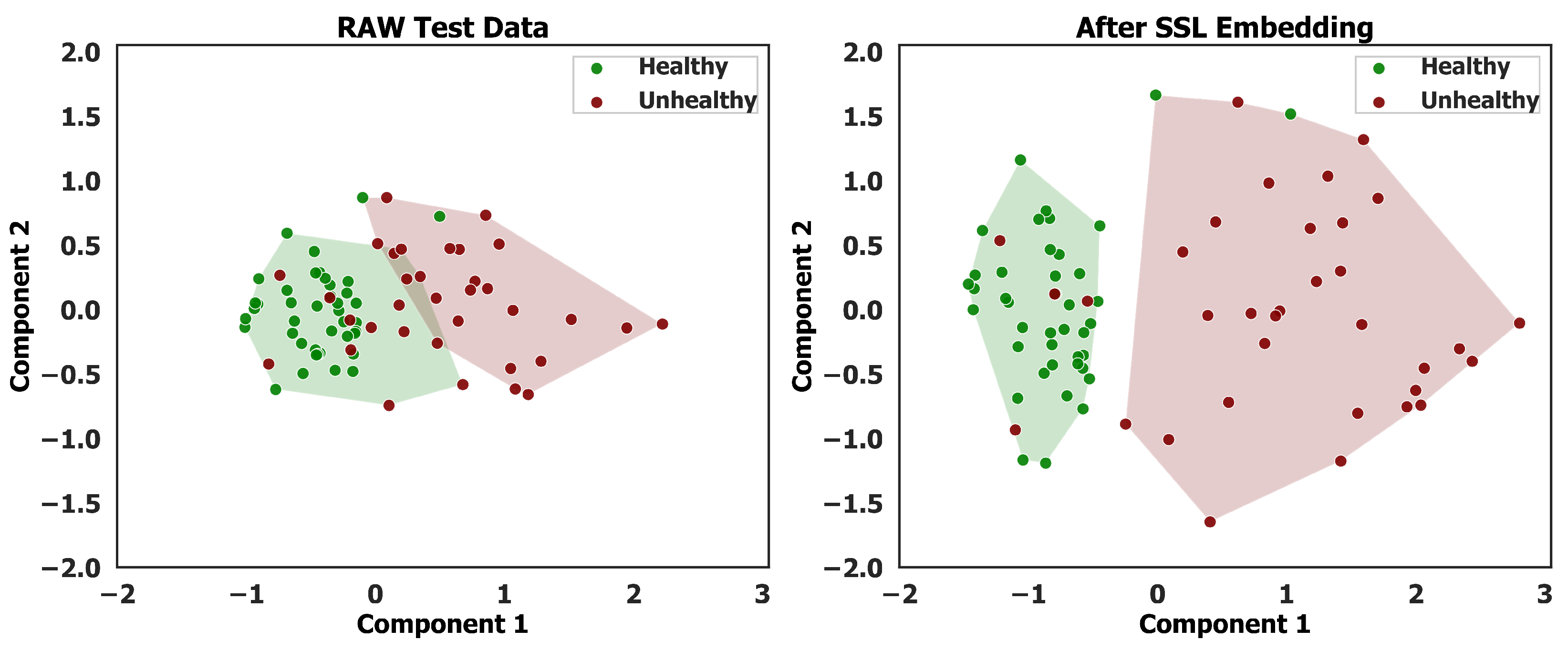
Figure 5 presents two scatter plots depicting the clustering of test data points, each characterized by 316 features. Principal Component Analysis (PCA) is employed to reduce the data’s dimensionality, enabling a visual representation of its distribution. The left plot illustrates the distribution of the raw test data, while the right plot represents the distribution after applying the SSL embedding technique outlined in Section 2.5. Both visualizations utilize the Agglomerative Hierarchical Clustering (AHC) algorithm to partition the soybean plots into two clusters, facilitating an assessment of clustering performance before and after embedding.

In the raw spectral space (Figure 5 (left)), considerable mixing occurs within cluster boundaries, with healthy and unhealthy samples frequently co-located. The Silhouette coefficient of 0.470 indicates moderate cluster quality, while the 3.1% convex hull overlap quantifies the ambiguous decision region. Following SSL embedding (Figure 5 (right)), cluster quality improves markedly (Silhouette: 0.526), with complete elimination of hull overlap. The 71.8% increase in centroid separation (1.20 to 2.06 units) further confirms enhanced feature discriminability. These quantitative improvements align with the 92% classification accuracy reported in Section 3.3, demonstrating that while SSL substantially enhances class separability, it appropriately maintains some boundary samples that reflect genuine spectral ambiguity in early-stage disease detection.

3.2. Clustering Performance Evaluation

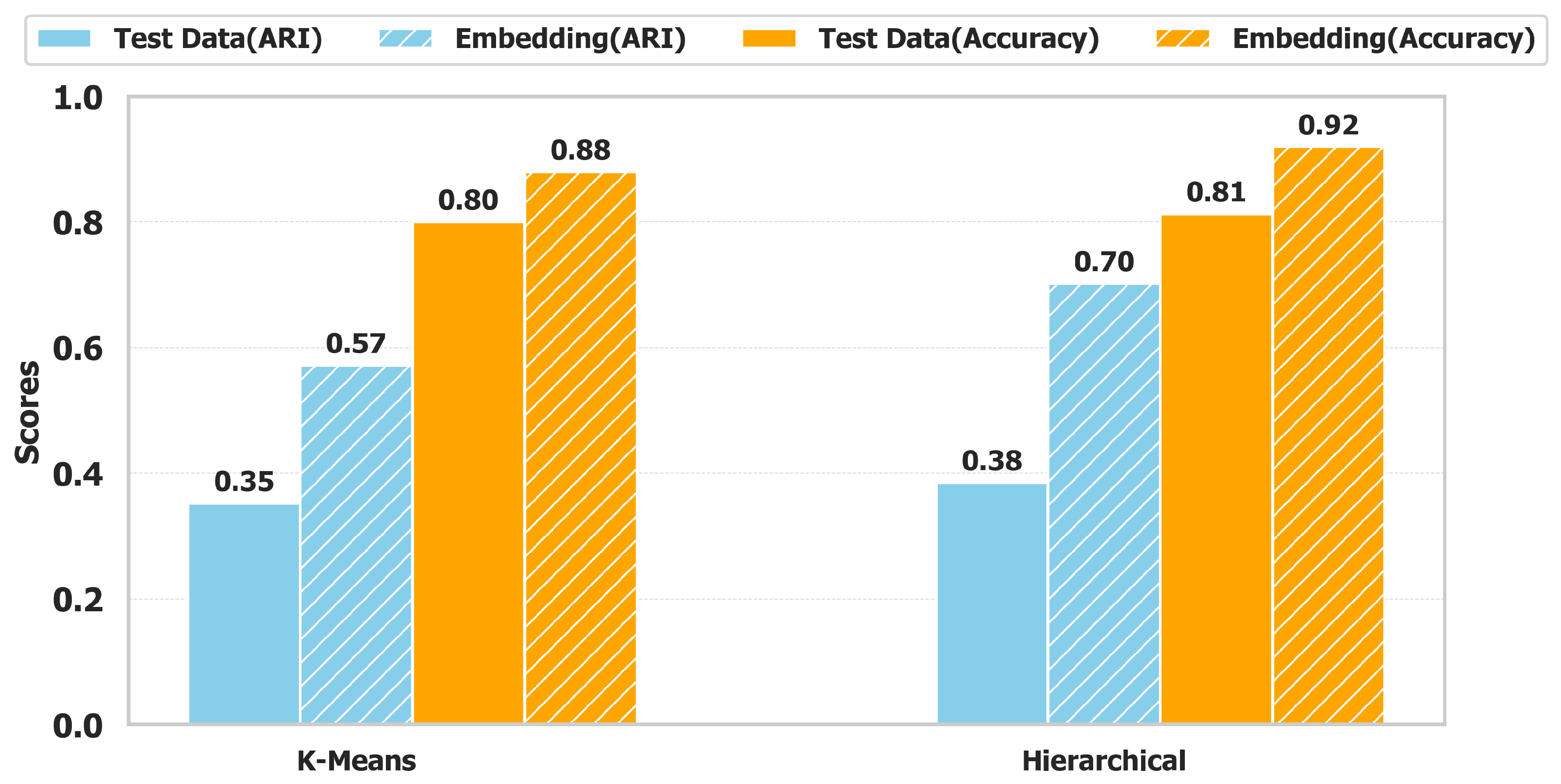
Clustering performance is evaluated using K-Means and AHC algorithms to assess the impact of the embedding technique on unsupervised classification. Figure 6 presents a comparative analysis between the raw test dataset and the embedded dataset, utilizing the Adjusted Rand Index (ARI) and Clustering Accuracy as evaluation metrics. The results highlight the substantial improvements achieved through embedding, demonstrating enhanced separability of the clusters.

For K-Means, ARI increases from 0.35 to 0.57, reflecting a 63% improvement, while for AHC, it rises from 0.38 to 0.70, an 84% gain. This enhancement indicates that embedding strengthens structural coherence in the feature space, reducing misclassification. Similarly, clustering accuracy improves notably. K-Means accuracy increases from 0.80 to 0.88, showing a 10% gain, while AHC improves from 0.81 to 0.92, achieving a 14% increase. These results demonstrate that embedding refines cluster compactness and inter-class separability, enabling better discrimination between healthy and unhealthy plots.

By restructuring the data distribution, SSL-based embedding mitigates intra-cluster variance while reinforcing inter-cluster distinctions. This transformation enhances decision boundaries, allowing clustering algorithms to produce more consistent and well-separated clusters, ultimately improving classification reliability in unsupervised plant disease detection.

3.3. Supervised Classification Performance

To evaluate the efficacy of the proposed SSL method, its performance was benchmarked against supervised learning models, including DNN, RF, and SVM. Hyperparameter configurations were selected to balance model capacity with generalization capability. The Random Forest classifier employed 500 decision trees with unrestricted maximum depth, resulting in an empirical mean depth of 9.1 ± 1.3 across training folds, trained directly on raw features without preprocessing. The SVM utilized an RBF kernel with regularization parameter $C=2.0$ and scale-based gamma $(1/(n_{features}\times var\left(X\right)))$, applied to standardized features (zero mean, unit variance). The DNN implemented with a six-layer fully connected architecture (Figure 4c) with ReLU activation, batch normalization on hidden layers, dropout regularization (p = 0.5) on the first two hidden layers, and Adam optimization (learning rate ${10}^{-3}$). DNN training employed early stopping with 25-epoch patience on a validation split (20% of training data), class-weighted cross-entropy loss, and a maximum of 300 epochs with batch size 256. Five-fold stratified cross-validation ensured robust generalization assessment.

As summarized in

Table 2. Performance comparison of supervised baseline models.

Model	Accuracy	Precision	Recall	F1-Score
DNN	0.89	0.90	0.89	0.90
RF	0.89	0.88	0.92	0.90
SVM	0.89	0.85	0.98	0.91
SSL (K-Means)	0.88	0.89	0.88	0.88
SSL (AHC)	0.92	0.91	0.92	0.92

, the SSL (AHC) model outperformed all comparators, achieving the highest accuracy (0.92), precision (0.91), and F1-score (0.92), thereby demonstrating enhanced feature extraction and clustering efficacy. The SVM exhibited the highest recall (0.98), indicating superior sensitivity in detecting positive cases. SSL (K-Means) showed comparatively lower performance, highlighting the advantage of AHC feature organization. These findings confirm that SSL-based embeddings yield more discriminative feature representations from unlabeled data, leading to improved generalization. The observed improvements of +3.4% in accuracy, +3.3% in precision, and +2.2% in F1-score compared to DNN and RF underscore SSL’s capability to capture structural dependencies effectively. This supports the utility of SSL as a robust alternative to conventional supervised learning, particularly in contexts with limited labeled data.

Beyond competitive accuracy, SSL’s key advantage lies in its annotation requirements. To quantify this, we evaluated supervised baselines trained on progressively reduced labeled subsets (10%, 25%, and 50%). Performance degraded substantially with decreasing labels, with RF accuracy dropping from 89.0% (50% labels) to 84.0% (10% labels), SVM from 89.0% to 86.0%, and DNN from 89.0% to 80.0% (Table S1). These results, averaged across five-fold cross-validation, demonstrate that supervised methods are highly sensitive to the availability of training data. In contrast, SSL achieves comparable accuracy (88–92%, Table 2) while requiring zero labels during training; the ground truth is used only to validate the clusters. This label-free learning addresses a fundamental challenge in early-stage disease detection: when visual symptoms are ambiguous and expert field assessments are resource-intensive, supervised methods struggle with insufficient training labels, whereas SSL learns directly from unlabeled spectral patterns. This operational advantage makes SSL particularly viable for real-world agricultural monitoring, where annotation bottlenecks limit supervised approaches.

3.4. Plot Level Prediction

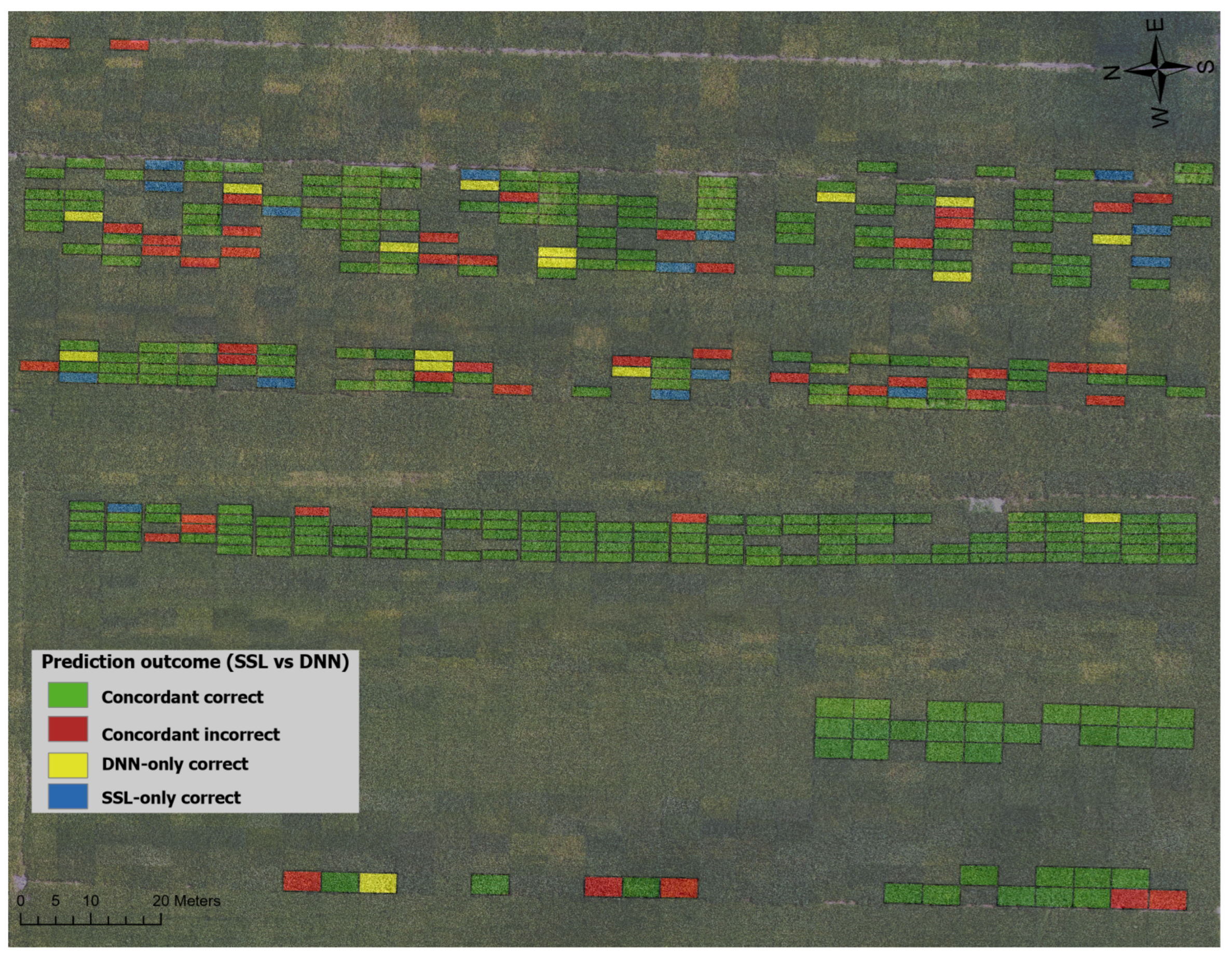
Figure 7 presents a comparative analysis of plot-level predictions generated by the SSL and DNN models on a soybean field. To ensure robustness and reliability, predictions were validated using K-fold cross-validation. The field is denoted into distinct plots, each color-coded to visualize prediction accuracy for both models, providing a spatial representation of their performance. This comparative mapping facilitates a comprehensive evaluation of the SSL method relative to a traditional supervised learning approach in assessing soybean plot health.

The results indicate a high degree of agreement between the two models, with both correctly predicting the plot health in 297 instances, as depicted by green plots. However, 47 plots were misclassified by both models, shown in red. Notably, in 16 cases, the SSL model misclassified plots that the DNN correctly predicted (blue), whereas in 15 instances, the DNN misclassified plots that the SSL correctly predicted (yellow). These discrepancies highlight the nuanced differences in model generalization and error patterns. Overall, the SSL model demonstrates performance comparable to the DNN model, despite operating without explicit supervision. This underscores its ability to leverage unlabeled data effectively, making it a viable alternative for classification tasks in scenarios where labeled data is scarce.

4. Discussion

The effectiveness of the proposed SSL framework for early SDS detection stems from its ability to leverage physiologically induced spectral separability without extensive manual annotation. While early-stage SDS produces subtle canopy-level stress signatures before visible symptoms emerge, these pre-visual changes create measurable reflectance shifts that our distance-based pairing strategy can exploit directly from unlabeled data. By learning to discriminate spectral patterns through contrastive representation learning, the framework achieves early detection sensitivity while circumventing the annotation bottleneck that constrains supervised approaches. This is particularly critical for SDS, where ground-truth labels during early infection are expensive and often inconsistent, even among expert observers.

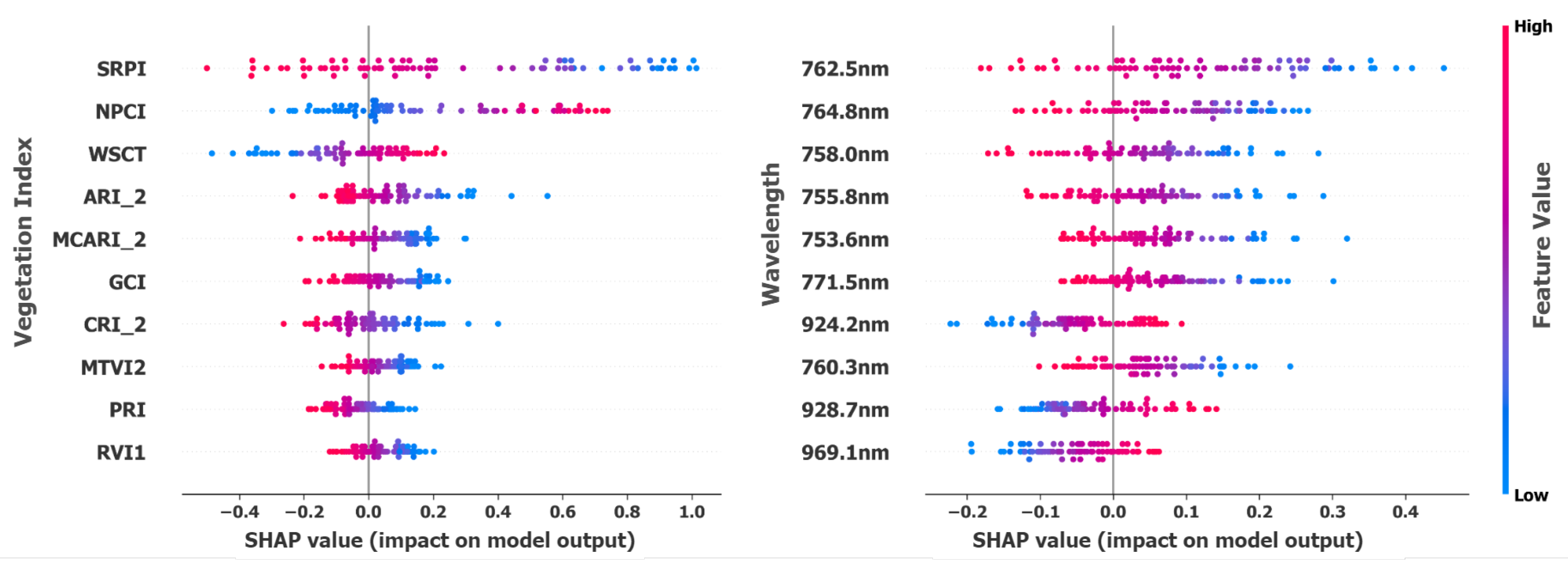
To elucidate the model’s decision-making process and identify key features driving soybean disease classification, a SHAP-based feature importance analysis was performed on hyperspectral bands and vegetation indices (VIs). This data-driven approach, unrestricted by predefined spectral categories, revealed the wavelengths and indices most critical for accurate discrimination.

Table 3. Top 10 most impactful vegetation indices with equations (wavelengths adapted to the sensor’s spectral ranges.

Index Name	Equation	Reference
Simple Ratio Pigment Index	$srpi={\displaystyle \frac{R_{430}}{R_{680}}}$	[41]
Normalized Pigment Chlorophyll Ratio Index	$npci={\displaystyle \frac{R_{680}-R_{430}}{R_{680}+R_{430}}}$	[42]
Water Stress and Canopy Temperature	$wsct={\displaystyle \frac{R_{970}-R_{850}}{R_{970}+R_{850}}}$	[43]
Anthocyanin reflectance index 2	$ar{i}_2=\left({\displaystyle \frac{1}{R_{550}}}-{\displaystyle \frac{1}{R_{700}}}\right)\times R_{800}$	[44]
Modified chlorophyll absorption ratio index 2	$mcar{i}_2={\displaystyle \frac{1.5\times [2.5\times (R_{800}-R_{670})-1.3\times (R_{800}-R_{550})]}{\sqrt{{(2\times R_{800}+1)}^2-(6\times R_{800}-5\times \sqrt{R_{670})}-0.5}}}$	[45]
Green chlorophyll index	$gci={\displaystyle \frac{R_{800}}{R_{550}}}-1$	[46]
Carotenoid reflectance index	$cri={\displaystyle \frac{1}{R_{550}}}-{\displaystyle \frac{1}{R_{700}}}$	[47]
Modified triangular vegetation index 2	$mtv{i}_2={\displaystyle \frac{1.5\times [1.2\times (R_{800}-R_{550})-2.5\times (R_{670}-R_{550})]}{\sqrt{{(2\times R_{800}+1)}^2-(6\times R_{800}-5\times \sqrt{R_{670})}-0.5}}}$	[45]
Photochemical reflectance index	$pri={\displaystyle \frac{R_{531}-R_{570}}{R_{531}+R_{570}}}$	[48]
Ratio vegetation index 1	$rv{i}_1={\displaystyle \frac{R_{810}}{R_{560}}}$	[49]

presents the top-ranked VIs, including $SRPI$, $NPCI$, $WSCT$, $AR{I}_2$, and $MCAR{I}_2$. These indices capture distinct physiological responses to SDS infection, such as $WSCT$ detecting water stress from impaired root water uptake, $AR{I}_2$ capturing stress-induced anthocyanin accumulation, $MCAR{I}_2$ reflecting chlorophyll degradation from nutrient deficiency, while $NPCI$ and $SRPI$ respond to pigment changes in the early stress stages. These results substantiate that the model’s predictions are grounded in physiologically relevant spectral responses specific to SDS pathogenesis.

Figure 8 presents the SHAP attributions for vegetation indices (VIs) and hyperspectral bands. Notably, red-edge (753–771 nm) and near-infrared (924–969 nm) bands were consistently highlighted. These spectral regions are directly linked to SDS pathophysiology, where Fusarium virguliforme colonizes soybean roots and produces toxins that disrupt vascular function, impairing nutrient and water transport to the canopy [19]. The red-edge region is particularly sensitive to chlorophyll content degradation resulting from nitrogen deficiency caused by impaired root nutrient uptake [46]. Similarly, NIR reflectance responds to reduced leaf water content and altered mesophyll structure when SDS compromises vascular water transport [50,51]. This correspondence between SHAP-selected features and established physiological stress markers confirms that the model’s predictions are grounded in biologically meaningful spectral responses rather than spurious correlations, reinforcing their diagnostic value for early SDS detection.

The co-occurrence of raw spectral bands and vegetation indices among top-ranked SHAP features indicates that both feature types contribute complementary information to classification performance. While raw bands (red-edge: 753–771 nm, NIR: 924–969 nm) capture direct physiological responses, vegetation indices encode nonlinear transformations (e.g., normalized difference ratios, soil-adjusted formulations) that emphasize specific stress signatures while suppressing confounding factors such as soil background and illumination variability. This suggests that the 316-feature representation (269 bands + 47 indices) provides multiple complementary perspectives on the underlying plant stress state, rather than redundant information. The presence of both feature types in the top-10 discriminative features supports the utility of vegetation index augmentation for enhanced separability in the SSL framework.

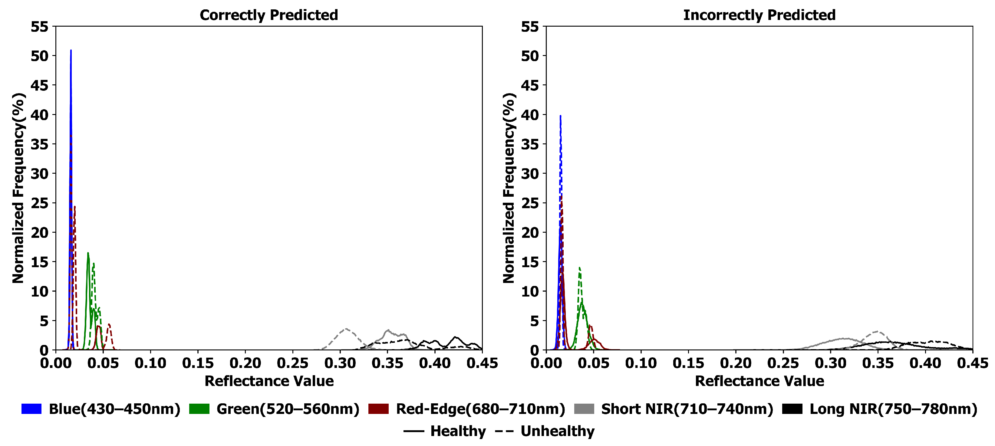
Reflectance frequency distributions (Figure 9) support these results by comparing correctly and incorrectly classified plots. Correctly classified samples show clear separation between healthy and diseased states in the red-edge and NIR regions, with healthy plots peaking near 0.09 and 0.40 reflectance, respectively, and diseased plots peaking lower. In contrast, blue and green regions exhibit significant overlap, indicating limited discriminative value. This highlights the importance of red-edge and NIR reflectance in disease detection. Misclassified plots demonstrate spectral overlap and increased variability in the blue, green, and red-edge regions, likely due to label noise and subtle disease progression. Such ambiguity stems from inconsistent ground-truth labels that inadequately reflect continuous spectral changes. Although NIR retains some separability, the increased noise emphasizes the need for uncertainty-aware techniques such as self-supervised denoising or contrastive spectral embeddings to improve feature reliability and reduce misclassification in UAV-based disease monitoring.

5. Conclusions

In this study, we developed a self-supervised learning (SSL) framework for the early detection of Sudden Death Syndrome (SDS) in soybean plants using UAV-based hyperspectral data. To enable effective representation learning from plot-level reflectance features, we introduced a distance-based pairing strategy and a modified contrastive loss function tailored to spectral data. The key contributions can be summarized as follows:

• An end-to-end SSL framework for SDS detection using UAV hyperspectral data, reducing reliance on in-situ measurements.
• A distance-based spectral pairing strategy that enhances cluster separability and strengthens feature learning.
• Demonstrated performance gains of 11% over unsupervised methods and 3% over traditional supervised learning, highlighting the efficacy of SSL for hyperspectral plant disease detection.

Model interpretability analysis using SHAP confirmed that the red-edge (753–771 nm) and NIR (924–969 nm) regions were the most critical spectral domains, consistent with known physiological stress markers. Reflectance-based separability further reinforced the diagnostic value of these bands, while errors were linked to spectral overlap and label noise. These findings demonstrate that SSL, coupled with targeted spectral feature selection, provides a scalable, interpretable, and label-efficient approach for precision agriculture.

While this study validates SSL on 375 plots from a single field site during the 2022 growing season, the framework’s design principles support broader applicability. The distance-based pairing strategy operates on standardized spectral features and employs adaptive quantile-based thresholds that instinctively adjust to data distribution, enabling methodological transferability across datasets. The reliance on universal physiological markers, red-edge and NIR bands corresponding to chlorophyll degradation and water stress, provides a biophysically grounded foundation that transcends site-specific characteristics. Cross-validation performance and the elimination of manual threshold tuning further demonstrate the framework’s robustness within the studied conditions. Nevertheless, systematic validation across diverse environmental contexts would strengthen operational confidence. Specifically, extending the framework to different soil types (Alfisols, Vertisols) would verify that the soil masking approach (Section 2.3) generalizes across pedological contexts. Multi-season deployment across varying phenological windows (V4–R1 early stages, R7–R8 late stages) would demonstrate temporal robustness under different climatic conditions and canopy architectures. Evaluating performance across broader disease severity ranges from pre-visual infection to severe foliar damage (>50%) would establish whether the distance thresholds ($\alpha =0.74$, $\beta =1.51$) generalize or require dataset-specific recalibration. Future work will focus on three key directions: (i) incorporating multi-temporal hyperspectral data to improve robustness and enable disease progression monitoring; (ii) extending the framework across diverse crops and environmental conditions to enhance generalizability; and (iii) integrating advanced SSL architectures and multi-modal fusion techniques to refine feature learning and improve classification performance across different disease stages.