Highlights
What are the main findings?
- Imaging laboratory spectroscopy in the longwave infrared (LWIR) range allows reliable and repeatable measurements of soil emissivity.
- Tests on different soils showed that the LWIR laboratory results agree well with outdoor measurements and mineral analyses.
What are the implications of the main findings?
- Our approach provides a weather-independent way to measure soils in the LWIR range and semi-quantify their minerology.
- It establishes a solid basis for calibrating satellite and airborne LWIR data, improving soil and environmental monitoring with the potential of becoming a standard protocol for these types of campaigns.
Abstract
This study introduces a controlled laboratory setup for hyperspectral longwave infrared (LWIR) imaging of soils, designed to bridge the gap between laboratory measurements and remote sensing observations. A Fourier-transform hyperspectral LWIR imaging spectrometer (Telops Hyper-Cam LW) was employed, together with a specialized heating plate, rigorous calibration protocols, and a Spatial Averaging Before Blackbody Fitting (SABBF) method to enable accurate LWIR indoor measurements. Unlike established laboratory techniques that measure reflectance and calculate emissivity indirectly, this setup enables direct passive measurement of soil emissivity, replicating airborne and spaceborne LWIR measurements of the surface. The emissivity spectra of 12 variable soil samples obtained with the lab setup were compared and validated based on LWIR Hyper-Cam LW spectra acquired under outdoor conditions, then were subsequently analyzed to determine the mineral composition of each sample. Spectral features and indices were used to estimate the relative content of quartz, clay minerals, and carbonates, from the most to least abundant. The results demonstrate that the laboratory-based setup preserves spectral fidelity while offering improved repeatability, scheduling flexibility, and reduced dependence on weather. Beyond replicating outdoor measurements, this controlled setup is easy to install and provides a reproducible framework for LWIR soil spectroscopy that could be considered for standard laboratory protocols, enabling reliable mineral identification, calibration/validation of airborne and satellite LWIR data, and broader applications in soil monitoring and environmental remote sensing.
1. Introduction
Soil is a complex medium with highly variable physical and chemical properties. It originates from weathered rocks of the Earth’s crust and undergoes continuous change. Soils contain plant debris, water, roots, small and large fauna, and minerals derived in situ or transported by runoff, dust storms, and human activity [1,2,3,4,5,6]. Several remote sensing techniques have demonstrated the ability to obtain information about soil surface composition. In particular, hyperspectral remote sensing, with high spectral resolution, in the visible and short-wavelength infrared ranges between 0.4 and 2.5 μm, has proven to be a valuable method of identifying and mapping soil characteristics, using sensors in laboratories, air-, and spacecrafts [1,2,3,4,5,6].
Recent research highlighted the additional value of the thermal infrared region, including the mid-wavelength infrared (MWIR, 3–5 μm) and long-wavelength infrared (LWIR, 8–12 μm) domains, for retrieving soil properties such as texture, carbon and nitrogen content, pH, and mineral composition when combined with statistical modeling [4,7,8,9,10,11]. In particular, Eisele et al. (2012, 2015) were able to quantitatively model Al2O3 and SiO2 content based on FTIR and MIDAC laboratory spectroscopy, using a Illuminator M4401 and a Perkin & Elmer Spectrum GX [8,9]. Notesco et al. (2019) demonstrated that outdoor ground-based hyperspectral LWIR measurements, based on the Telops Hyper-Cam LW, were used to derive semi-quantitative estimates of quartz, clay minerals, and carbonates from soil emissivity spectra, with results in good agreement with XRD mineralogy [4]. Note that quantitative mineral estimates provide precise, reproducible concentrations of minerals (usually expressed in weight %, molar ratios, or absolute values) based on calibrated analytical techniques, and semi-quantitative estimates give approximate relative abundances or ranges, derived from indirect proxies, and are useful for rapid screening but not for definitive concentration calculations [12].
Despite these advances, a methodological gap remains between laboratory measurements and remote sensing observations. Conventional laboratory approaches typically rely on reflectance-based measurements with indirect emissivity estimation, while outdoor LWIR measurements are weather-dependent and logistically demanding. A standardized protocol for controlled laboratory acquisition of direct emissivity spectra using hyperspectral LWIR imaging is currently lacking. Addressing this gap is essential for producing reproducible reference spectra that are directly comparable to airborne and satellite LWIR observations.
This study introduces a laboratory-based protocol for measuring soil emissivity spectra using hyperspectral LWIR imaging. The method employs the Telops Hyper-Cam LW sensor under controlled indoor conditions, enabling direct emissivity measurements comparable to outdoor acquisitions. Validation was performed by comparing the laboratory-based emissivity spectra obtained with emissivity spectra of the same soil samples acquired under a different protocol in outdoor conditions. Furthermore, mineralogical indices developed by Notesco et al. (2019) were used to validate the mineralogical identification of the soil samples [4]. The proposed setup allows the generation of reliable ground-truth spectra, independent of weather constraints, using the same instrument applied in airborne campaigns, providing a reproducible and flexible workflow for soil compositional analysis.
2. Materials and Methods
2.1. Soil Samples and Mineral Abundance
Twelve soil samples (see Table 1) from the legacy soil spectral library of the Tel-Aviv University (Israel) were selected for this study [13,14]. The samples represent diverse formation conditions, including differences in climate, parent material, and topography. All samples were collected from the surface layer (0–5 cm) at multiple sites across Israel, air-dried and crushed to a grain size of ≤2 mm. These soils have previously been characterized in the context of outdoor hyperspectral LWIR measurements by Notesco et al. (2019) [4], providing a basis for direct comparison between laboratory-based and outdoor-derived emissivity spectra.

Table 1.
Soils and their mineral abundance.
2.2. Laboratory Setup
Laboratory measurements were carried out using the Hyper-Cam LW imaging spectrometer. The Hyper-Cam LW is a lightweight and compact imaging radiometric Fourier-transform spectrometer (FTIR) built by Telops, Quebec, QC Canada, and covers a range from 7.6 to 11.7 μm (see Table 2) [15,16]. It is based on a Michelson interferometer coupled to a 320 × 256 longwave infrared photovoltaic MCT (mercury-cadmium-telluride) focal plane array detector, with a user-adjustable field of view (FOW) [15,16,17]. The instrument offers a selectable resolution ranging from 0.25 to 150 cm−1. Each pixel of the images contain the complete spectrum and have an instantaneous field of view of 0.35 mrad [15,16,17]. The Hyper-Cam LW features two calibration blackbodies mounted in front of the instrument to perform a complete end-to-end radiometric calibration of the infrared measurements [15,16,17]. Besides acquisition electronics, it also includes processing capabilities, and is able to convert the raw interferograms into radiometrically calibrated spectra using a real-time discrete-Fourier transform (DFT) technique [15,16,17]. Its weatherproof enclosure provides operability in harsh environments from −10 °C to +45 °C [16].
Table 2.
Telops Hyper-Cam LW sensor specifications [15,16,17].
For the laboratory measurements, the Hyper-Cam LW was mounted on a stable and adjustable tripod designed for the instrument. Around 10 g of dried soil sample material was placed in each aluminum sample holder. The soil samples were then placed on a custom laboratory heating plate set to 80 °C for continuous heating prior and during measurement, while the camera was equipped with a wide-angle ×0.25 telescope and gold mirror form Telops, Quebec, QC, Canada to provide an adequate nadir field of view (FOV) (see Figure 1 and Figure A5). The aluminum sample holders here have the purpose of transferring the heat from the plate to the soil sample material. Heating prior to measurement was applied until thermal equilibrium was reached, monitored by a thermocouple placed at the soil surface (see Figure 2). The 10 g of soil sample material usually reached their maximum temperature in under 15 min of heating. An amount of 10 g was chosen as this was enough soil for all samples to cover the sample holder surfaces while at the same time reaching stable temperatures in a sensible amount of time. Heating of the samples creates a thermal contrast between the samples and the laboratory surrounding. This improves the signal-to-noise ratio of the measurements as the downwelling radiance from the air-conditioned (20 °C) environment is smaller in relation to the signal from the samples. The higher the temperature difference, the lower the relative influence of the background radiation of the surroundings on the at-sensor radiance signal of the samples.
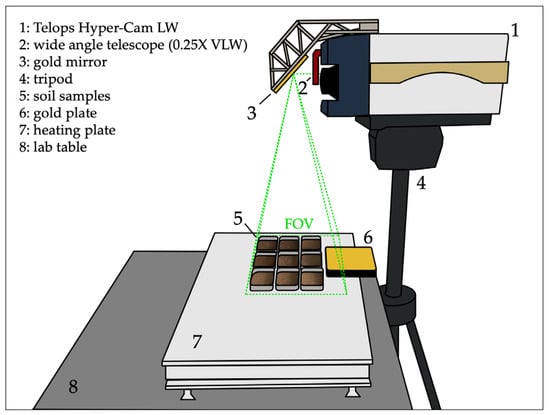
Figure 1.
Schematic of the laboratory setup for hyperspectral LWIR imaging with the Telops Hyper-Cam LW. The instrument (1) is mounted on a tripod (4) and equipped with a wide-angle 0.25× telescope (2) and a gold mirror (3) to enable nadir acquisition. Soil samples (5) are placed on a laboratory heating plate (7) alongside a reference gold plate (6). The field of view (FOV) of the camera is indicated by the dotted green lines. All components are arranged on a laboratory table (8) in an air-conditioned room.
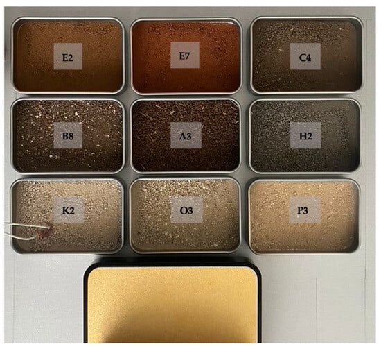
Figure 2.
Top view of soil samples (with sample labels in gray), arranged for measurements with the gold plate for measuring downwelling radiance located in the lower center of the image. In the bottom left sample, a temperature sensor (thermocouple) for soil surface temperature validation is visible—nadir photograph.
The 80 °C plate temperature was selected in order not to alter soil structure while producing soil surface temperatures of approximately 60–70 °C and creating a sufficient temperature contrast between the samples and the laboratory. Such soil surface temperatures are also reached, or even exceeded, under natural conditions in Mediterranean and Middle Eastern climates during sunny summer periods [18,19,20]. Laboratory-based LWIR images were subsequently acquired with the Telops Hyper-Cam LW, covering the 7.9–11.5 µm range with 124 spectral bands at a resolution of 4 cm−1. This resolution was chosen to increase the signal-to-noise ratio while keeping a good enough spectral resolution to resolve the mineralogical features. Furthermore, it is stated to be the optimal resolution for the system and is often used in remote sensing applications during, e.g., airborne acquisitions and/or their ground/sample validation [21,22].
2.3. Data Pre-Processing
The processing of the Hyper-Cam data involved blackbody calibration using Reveal Calibrate 5.3.1, wavenumber to wavelength conversion, temperature emissivity separation (TES), and downwelling radiance correction using a Python 3.12 algorithm described in the next sections.
The wavenumber (wn) to wavelength conversion is performed via a Python algorithm that converts the spectral radiance via pixel-by-pixel iterations by applying Equation (1).
where .
2.3.1. Laboratory TES Using a Blackbody Fitting Approach
The at-sensor radiance measured for each soil pixel in the LWIR image contains contributions from both temperature and emissivity. The emissivity spectrum was derived by applying a self-developed Temperature Emissivity Separation (TES) procedure implemented in Python, as described below:
The emissivity spectrum of the surface, reflecting its chemical and physical properties, can be calculated using Equation (2), where is the observed at-sensor radiance, is the blackbody radiance, is the emissivity, is the atmospheric transmittance, is the downwelling radiance, and is the upwelling radiance, with all factors at temperature and wavelength .
Under laboratory conditions, the atmospheric transmittance is equal to 1 and the upwelling radiance is negligible due to the very short sensor-target distance, simplifying Equations (2) to (3).
Equation (3) can be rearranged for emissivity calculations, accounting for downwelling radiance, as shown in Equation (4) [23].
Equations (3) and (4) are used as part of our Python processor for hyperspectral radiance images. The program calculates the temperature and emissivity for each pixel as follows.
First, constants (Planck’s constant, Boltzmann’s constant, and the speed of light) are defined for blackbody radiation calculations. An initial temperature T, based on the heating plate, is used to generate the first blackbody curve. This curve is iteratively fitted by adjusting temperature to match the measured radiance. The wavelength array, defined from the image header, provides the basis for modeling the Planck function and performing TES.
The Planck function calculates blackbody spectral radiance for temperature T over the defined wavelength range, while its inverse is used to estimate brightness temperature from . For each pixel, the brightness temperature is derived using the inverse Planck function, ensuring that blackbody radiance at this temperature is greater than or equal to the pixel radiance. The temperature inversion is performed by minimizing the residual between the observed radiance spectrum and the Planck function using the “fsolve” function provided by the Python package SciPy [24]. The SciPy “fsolve” function is a Python wrapper for MINPACK’S “hybrd” and “hybrdj” algorithms, which are based on Powell’s hybrid method, an iterative optimization approach for non- linear functions and a variant of gradient descent [25,26,27]. Specifically, we define the cost function (5) as follows:
and solve for the temperature that minimizes . This corresponds to the brightness temperature, i.e., the blackbody temperature that best fits the observed spectrum. Because the observed radiance is a product of soil temperature and emissivity, the brightness temperature is not yet the true soil temperature. However, it provides a physically consistent upper bound: emissivity depresses the spectrum below the blackbody curve, so the temperature that minimizes residuals represents the soil temperature prior to emissivity correction.
The measured downwelling radiance is taken from a gold plate in the scene, identified either by thresholding or predefined coordinates. This represents the radiation incident on the sample from laboratory surroundings and is essential for accurate emissivity retrieval. The emissivity ε(λ) for each pixel is calculated as the ratio of measured radiance to the blackbody radiance at the estimated temperature, corrected for L↓(λ) according to Equation (4). Then the algorithm iteratively adjusts the fitted blackbody curve in 0.05 K steps until it exceeds the observed radiance at all wavelengths, following the approach of Notesco et al. (2014), outputting the adjusted temperature and emissivity images [28].
In summary, this implementation estimates temperature and emissivity from hyperspectral LWIR radiance images involving the use of Planck’s law, the concept of blackbody radiation, and the Temperature Emissivity Separation (TES) by blackbody fitting. The brightness temperature is calculated using the inverse Planck function, and the emissivity is estimated by fitting the observed radiance to the blackbody radiance at the estimated temperature. The code also includes corrections for downwelling radiance. The output consists of temperature and spectral emissivity images (see Figure 3).
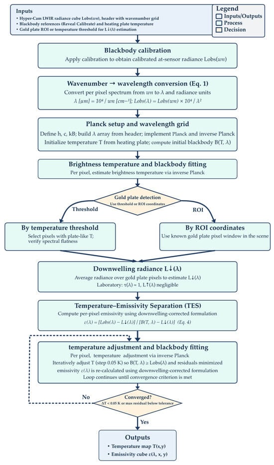
Figure 3.
Flowchart of the processing algorithm.
2.3.2. Automated ROI Extraction
The calculated emissivity data from the measurements of the samples were processed using an automated Region of Interest (ROI) Python algorithm that detects the samples in the emissivity images using object detection, based on OpenCV edge detection (see [29]). When provided with a sample names text file, it extracts 70 × 40-pixel ROIs from the center of each sample tray (see Figure 4). The extracted sample ROIs are then stored as individual hyperspectral emissivity data cubes containing 70 × 40 pure sample pixels without sample tray edges. Another Python script then averages the 70 × 40-pixel image cubes to obtain a single emissivity curve for each sample. The resulting emissivity curve of each sample is hence a 70 × 40-pixel average.
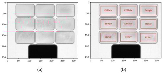
Figure 4.
(a) Band 124 of the radiance data (in wavelength format) is used by the OpenCV edge detection algorithm to identify the shapes of the sample boxes and extract 70 × 40-pixel ROIs of the samples; (b) the auto detected and extracted samples are shown (ROIs in red).
2.3.3. Spatial Averaging Before Blackbody Fitting (SABBF)
In addition to the ROI-based workflow described above, a modified processing chain was implemented to further improve the signal-to-noise ratio (SNR) of the radiance data prior to emissivity retrieval. This method, termed Spatial Averaging Before Blackbody Fitting (SABBF), applies spatial filtering before the TES step. After ROI detection, the radiance data of each sample was averaged using a 10 × 10 pixel running average filter. This procedure reduces high-frequency noise in the radiance domain by combining the hyperspectral radiance of adjacent pixels. Although the image dimension per ROI remains at 70 × 40 pixels, the effective spatial resolution is reduced to 7 × 4 pixels (Figure 5). The noise-suppressed radiance spectra were then processed using the blackbody fitting algorithm described in Section 2.3.1. A comparison of emissivity retrieval from standard pixel-level fitting versus SABBF-processed data is shown in Figure 6, demonstrating the improvement in spectral smoothness and stability.
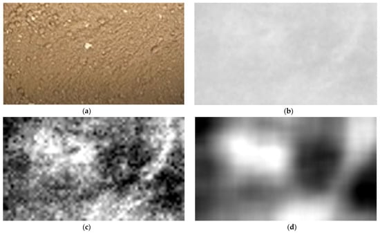
Figure 5.
(a) Nadir RGB photograph of the soil sample P3 (Torriorthent); (b) sample P3 (Torriorthent) radiance of band 124 at 70 × 40 pixels; (c) sample P3 (Torriorthent) radiance of band 124 at 70 × 40 pixels, with enhanced contrast; and (d) sample P3 Torriorthent 70 × 40 pixel radiance of band 124, with enhanced contrast and averaged by 10 × 10 pixel running filter.
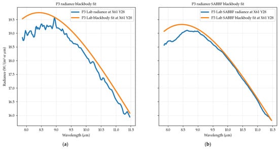
Figure 6.
The radiance of P3 Torriorthent (blue lines) of the unaveraged data of one selected Pixel at (X: 61, Y: 28) in sample P3 Torriorthent (a), and the 10 × 10 pixel radiance average (+/−5 pixels) centered at (X: 61, Y: 28) (b), and their corresponding blackbody fits (orange lines). The plot shows that spatial averaging prior to blackbody fitting leads to a closer fit and hence the area between calculated blackbody (orange) and radiance (blue) of the data is smaller and less influenced by noise, leading to a more exact estimate of the emissivity of the material.
2.4. Validation with Outdoor Lab Measurements
For the validation of our method we chose samples that have been measured outdoors with the same instrument (Telops Hyper-Cam LW) before by Notesco et al. (2019) (see Section 2.1) [4]. The data collected by Notesco et al. (2019) has been processed by a slightly different algorithm using Interactive Data Language (IDL), described in detail in Notesco et al. (2014) [4,28]. The differences are considered minor because both the blackbody fitting and TES algorithms use a generally similar approach, differing primarily in terms of mathematical processing details. The main distinction occurs in the outdoor measurements, where atmospheric downwelling correction is required to account for environmental influences. The general physical foundation of the blackbody fitting and the related mathematics of the formulas in Section 2.3 are given in both approaches and we consider the outdoor data measured by Notesco et al. (2019) to be similar enough to validate our indoor laboratory method [4].
2.5. Mineralogical Identification
The mineralogical characterization of the laboratory-measured soil samples was conducted using indices derived from known emissivity absorption features of specific minerals as also described in Notesco et al. (2019) [4]. A triplet-like absorption feature between 8.00 µm and 10.40 µm, with minima at 8.25 µm, 8.79 µm, and 9.35 µm, indicates the presence of both quartz and clay minerals. A decrease in the amount of quartz with an increase in the amount of clay minerals shifts the main absorption to 9.00–10.40 µm, with a minimum at 9.58 µm. On the other hand, a minimum in the 8.00–8.18 µm range and/or a noticeable absorption feature between 10.11 µm and 11.38 µm indicates the presence of carbonates in the soil. These mineral-related emissivity features were used to create spectral indicants, described in Table 3, to identify the most abundant mineral(s) in each soil sample.
Table 3.
Spectral indicants of minerals.
Next, two indices (Formulas (6) and (7)) were created to identify the less abundant minerals in each soil sample:
where Nε is the normalized emissivity value at the indicated wavelength.
SQCMI (Soil Quartz Clay Mineral Index) = Nελ=9.58 µm/(Nελ=8.25 µm × Nελ=8.79 µm)
SCI (Soil Carbonate Index) = Nελ=11.22 µm × Nελ=10.56 µm/Nελ=8.79 µm
A higher SQCMI value corresponds to a greater proportion of quartz compared to clay minerals, while a lower SCI value reflects a higher carbonate content within the soil sample [4]. The indicants based on these indices are described in Table 4.
Table 4.
Spectral indicants of relative amounts of minerals.
2.6. Statisical Analysis
Further statistical analysis has been performed by calculating statistical indicators between the outdoor and SABBF measurements. The , the , and the have been calculated for the laboratory-acquired SABBF data and the outdoor measurements according to Formulas (8)–(10):
where is the covariance between the two spectral datasets, and and are their standard deviations.
where and are corresponding values of the two spectral measurements, and is the number of spectral bands.
3. Results
3.1. Emissivity Spectra
In order to provide a proof of concept of the laboratory measurement setup with the thermal hyperspectral imaging system and heating plate, 12 soil samples, also present in the legacy soil spectral library of Israel and measured in an outdoor setup by Notesco et al. (2019) (see Section 2 and [4]), were measured and compared.
Figure 7 shows the emissivity spectra of selected soil samples, highlighting mineral-related features. As descried above in Section 2.5, the triplet-like absorption features between 8.00 µm and 10.40 µm indicates the presence of both quartz and clay minerals, which can be seen in soil E7. In soil H2, a shift in the main absorption feature to 9.00–10.40 µm correlates with a decrease in quartz towards an increase in clay minerals. In sample K2, the presence of carbonates is indicated by the positive slope between 8.00 µm and 8.40 µm, with absorption between 10.20 µm and 11.40 µm.
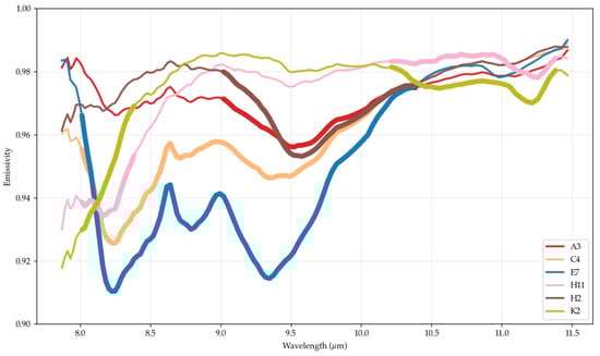
Figure 7.
Emissivity spectra of selected soil samples, bold curves represent mineral-related features mentioned in the text.
The samples E2, E7, C4, B8, A3, H2 represent soils that are quartz-rich to clay mineral-rich. Comparing the spectra from these soils show that the lab measurements can reproduce the outdoor measurements very well (Figure 8). There are little to no noticeable absorption position differences. The most quartz rich samples E2 and E7 both show the typical triplet-like absorption feature with minima at 8.21 µm, 8.85 µm, and 9.33 µm, associated with both quartz and clay minerals. The overview of all samples measured in the lab and under outdoor conditions shows that the general absorption features and characteristics of the soils can be reproduced via the laboratory measurements (see Figure 8 and Figure A1).
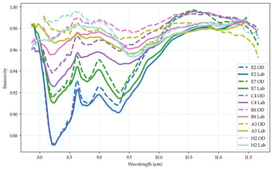
Figure 8.
Comparison of laboratory measurements (Lab) vs. outdoor measurements (OD) of 6 samples from the TAU spectral library.
3.2. Impact of Spatial Averaging Before Blackbody Fitting (SABBF)
The Spatial Averaging method (SABBF) is used to extract the data prior to blackbody fitting and the application of a running filter before the data is processed by the blackbody fitting algorithm, and has some advantages and disadvantages, depending on the sample nature and specific use case. The running filter reduces the spatial resolution information, resulting in spatially blurred images of the samples, making spatial surface features and textures of the individual samples less resolved and harder to detect. When spatial surface features or structures of samples are of interest, this is a major disadvantage of the method. This would be the case if, for example, rock samples or structurally preserved soil samples are measured when spatial surface structures are of interest.
In our case, the spectral information is more important and the resulting radiance data per pixel is smoother and less noisy after the averaging filter is applied. This enables the simulated blackbody, as described in Section 2.3.3., to be fitted closer to the radiance curve of each pixel of the sample, allowing a more precise emissivity estimation by the algorithm. For the purpose of building a spectral emissivity soil library where the results are only spectra without spatial information, the averaging method presents a way to further improve the blackbody fitting, resulting in a closer estimation of the true emissivity of the soil samples. The comparison of all samples that have been measured in the laboratory setting and then processed by the standard blackbody fitting approach and the SABBF method show that the overall calculated emissivity is generally slightly higher (see Figure 9, Figure 10, and Figure A2).
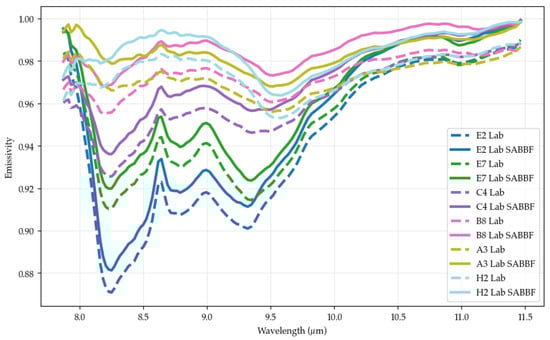
Figure 9.
Comparison of the laboratory measurements of samples E2, E7, C4, B8, A3, and H2 with the standard blackbody fitting TES (Lab) vs. the average values before the blackbody fitting TES method is applied (Lab SABBF).
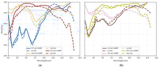
Figure 10.
Comparison of SABBF emissivity spectra from laboratory (Lab, solid lines) and outdoor (OD, dashed lines) results—(a): samples E7, H2, and K2; (b): samples C4, A3, and H11.
3.3. Mineralogical Identification and Semi-Quantification
The laboratory-based emissivity spectra processed with the SABBF method resembles the outdoor-based spectra regarding the mineral-related features. These emissivity features were used to calculate indicants and indices created by Notesco et al. (2019) and are described in Table 3 and Table 4, and were also used to determine the content of quartz, clay minerals, and carbonates in each soil in a semi-quantitative manner, from more to less abundant minerals (Table 3) [4]. Laboratory-based classification regarding the most abundant mineral fit the outdoor-based classification, as well as the XRD analysis results, for all soil samples. Regarding the less abundant minerals, the laboratory-based classification fit the outdoor-based results of most (75%) soil samples (Table 5). It should be noted that soil moisture may affect the results, as well as organic tissues such as litter, and particularly lignin (e.g., Elvidge 1988) [30]. Nonetheless, all soils were air-dried and exposed to heat conditions that minimize any moisture effects. The organic carbon content of these arid and semi-arid soils was very low (Table 1), and the existing organic matter was already decomposed into humus, which is not expected to significantly influence the LWIR spectrum.
Table 5.
Content of quartz (Q), clay minerals (CMs), and carbonates (Cs) in soil samples. Letters in bold represent the most abundant mineral.
3.4. Statistical Agreement Between SABBF and Outdoor Measurements
The comparison between the SABBF laboratory emissivity measurements and the outdoor spectra shows a consistently high agreement across most of the LWIR atmospheric window (Figure 11). Band-wise correlation coefficients remain above 0.95 for the majority of channels between 8 and 10.5 µm, with corresponding RMSE values typically below 0.006 (Figure 12), indicating that both systems capture the same spectral structure and sample-to-sample variability with high fidelity. This behavior is also reflected in the overall scatter analysis, where emissivity values from both setups align closely along the 1:1 line, yielding an overall coefficient of determination of r2 = 0.91 and an RMSE of 0.0079 (Table 6 and Figure 13). Systematic deviations emerge toward the long-wavelength end of the spectrum, and from approximately 10.6 µm onward, correlations decrease markedly and RMSE increases beyond the 1% emissivity threshold (Figure 12), with the strongest discrepancies occurring between 11.0 and 11.5 µm. The detailed per-band scatter plots provided in Appendix A, Figure A6, Figure A7, Figure A8 and Figure A9, confirm these patterns, showing tight agreement in the 8–10.5 µm range and increasing departure from the 1:1 line at longer wavelengths. A small but consistent negative bias of –0.004 indicates that the outdoor measurements tend to underestimate emissivity relative to the SABBF measurements in this region. Overall, the two systems demonstrate excellent agreement across the diagnostically important part of the LWIR window, with notable wavelength-dependent degradation at the spectral longwave edge.
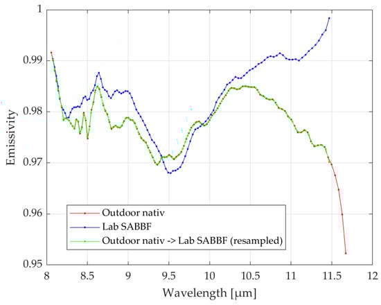
Figure 11.
Spectral comparison between the average of the SABBF laboratory emissivity measurements. Red line: average of the outdoor measurements. Blue line: average of the SABBF measurements. Green line: average of the outdoor measurements resampled to the exact SABBF band positions.
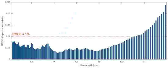
Figure 12.
Band-wise RMSE values of spectral emissivity.
Table 6.
Overall coefficient of determination, RMSE and MAE for the SABBF, and outdoor measurements.
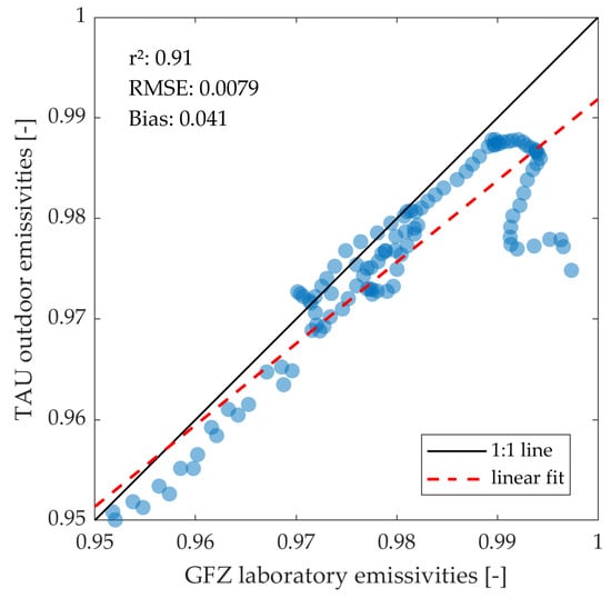
Figure 13.
Scatter analysis of the emissivity values of the outdoor and SABBF measurements.
4. Discussion
The strong agreement across the 8–10.5 µm spectral range suggests that differences between the indoor laboratory and outdoor measurement setups have minimal impact on the retrieval of key silicate-related emissivity features that underpin most LWIR-based soil mineralogical applications. The deviations observed beyond approximately 10.6 µm (Figure 11 and Figure 12) can likely be attributed to a combination of physical and instrumental constraints inherent to open-sky emissivity measurements. Increased atmospheric absorption and emission toward the long-wavelength end, combined with the lower signal-to-noise ratio of FTIR-based sensors in this region, make downwelling radiance correction particularly sensitive to small temperature inaccuracies or calibration residuals. Differences in calibration workflows may further amplify these effects, leading to the systematic underestimation of emissivity in the outdoor spectra documented in Appendix A, Figure A6, Figure A7, Figure A8 and Figure A9, and summarized in the overall scatter plot (Figure 13). For downstream soil property estimation, these wavelength-dependent biases imply that spectral features in the 11–11.5 µm region should be used with caution or excluded when merging datasets from different measurement setups. Nevertheless, because the most diagnostic absorption features for quartz, feldspar, and clay minerals lie within the high-agreement region, the overall implications for soil mineral, texture, and related property estimation are expected to be moderate, provided that modeling approaches down-weight or mask affected long-wavelength bands. The primary difference between indoor and outdoor measurements lies in the consistency and control of the experimental conditions. Indoor measurements offer several advantages over outdoor and existing laboratory protocols for LWIR emissivity measurements. Firstly, the protocol is both cheap and easy to implement if a hyperspectral thermal imaging system is available, making it accessible for various laboratories. Secondly, it is easy to replicate, ensuring that different labs can achieve consistent results. Unlike FTIR spectroscopy, which analyzes soil samples in a different manner, this method allows soil samples to be analyzed in their own volume. This approach ensures that the emissivity measurements are more representative of real-world conditions, replicating air/spaceborne measurements. Additionally, the use of standard TES and adapted spatial averaging techniques allows for the derivation of high-quality emissivity data.
Despite the advantages, comparing measurements taken under such different conditions as indoor and outdoor remains challenging. The differences in emissivity, absorption depth, and mineral indices could be due to slight differences in the processing algorithm, and/or due to the fact that the sample mixtures surface exposure was composed slightly differently. A rather unlikely explanation would be chemical changes as a result of storage time, as the long-term stability of soil sample characteristics has been demonstrated in a recent study by Shepard et al. (2024) [31]. The re-arrangement of particles at the soil surface and varying atmospheric conditions can lead to discrepancies in the data. Considering the comparison of the standard blackbody fitting approach, the SABBF method, and the outdoor measurements, it can be shown that the SABBF method brings the laboratory measurements closer to the outdoor measurements in terms of the general shape of the emissivity (see Figure 10, Figure A3 and Figure A4). The results of this study indicate a very good agreement between the two types of measurements, validating both methods. This agreement suggests that while indoor measurements provide a controlled and reproducible environment, they can still produce results that are consistent with outdoor measurements, thereby bridging the gap between laboratory and field data.
5. Conclusions
A laboratory setup protocol is presented that utilizes a heating plate, calibration and temperature measurements, blackbody fitting, and a TES processor with spatial averaging to improve signal-to-noise ratio. This approach is used to obtain LWIR spectral emissivity data for 12 soil samples with varying mineralogical compositions. Data acquisition and processing are validated by comparing them with outdoor measurements of the same samples (see [4]). This replication is crucial for ensuring the reliability and consistency of data collected under different environmental conditions. The Spatial Averaging (SABBF) method further aligns the emissivity of lab measurements with those of outdoor soils. By leveraging this method, we can ensure that the emissivity values obtained in a controlled indoor environment are well concordant with those measured in natural outdoor settings. Furthermore, mineralogical identification and semi-quantification was derived and compared with XRD analyses. A good concordance was obtained, due to the well resolved mineralogical features in the spectra.
Producing ground-truth spectra indoors under any weather conditions with the same instrument used for aerial acquisition enhances our workflow in remote soil compositional analysis. This capability allows for more flexible scheduling and reduces dependency on favorable weather conditions that are necessary for outdoor measurements. Furthermore, it ensures that the data collected are consistent and comparable across various study sites and temporal frames. The ability to conduct thorough analyses indoors also provides opportunities to refine methodologies and validate hypotheses before conducting extensive fieldwork, thereby optimizing resources and time. The protocol developed is suggested as a foundation for a standard laboratory protocol for LWIR measurements and could be easily followed in different laboratories.
The integration of controlled lab measurements with aerial acquisition instruments bridges the gap between laboratory research and practical field applications. This approach promotes the development of more robust soil classification models, which can be applied to monitor and manage agricultural lands, assess soil health, and track environmental changes over time. By combining precise laboratory techniques with advanced remote sensing technologies, we can achieve a deeper understanding of soil properties and dynamics across diverse landscapes.
Author Contributions
Conceptualization, H.L.C.D., R.M. and S.C.; methodology, H.L.C.D.; software, H.L.C.D.; validation, H.L.C.D. and G.N.; formal analysis, H.L.C.D., R.M. and G.N.; investigation, H.L.C.D. and R.M.; resources, R.M., S.C. and E.B.-D.; data curation, H.L.C.D., R.M., S.C., G.N. and E.B.-D.; writing—original draft preparation, H.L.C.D.; writing—review and editing, R.M., S.C. and G.N.; visualization, H.L.C.D.; supervision, R.M. and S.C.; project administration, R.M. and S.C.; funding acquisition, S.C. All authors have read and agreed to the published version of the manuscript.
Funding
This work was supported by funding from the GFZ Helmholtz Centre for Geosciences POF-IV research program topic 5 (Future Landscapes) and from the Helmholtz Association within the (heatwave) MOSES (Modular Observation Solutions for Earth Systems) research infrastructure. Additional financial support was provided by the NextSoils project funded by the European Space Agency SUP-1 program (Contract No. 4000145828/24/I-DT-bg).
Data Availability Statement
The laboratory data is available upon request.
Acknowledgments
H.L.C.D. gratefully acknowledges the financial support received from the GFZ POF program “Landscape for the future” and the additional support received from ESA Contract No. 4000145828/24/I-DT-bgh from “NextSoils+”. The GFZ’s Telops Hyper-Cam LW was acquired through the MOSES observing system of the Helmholtz Research Field “Earth and Environment”, as part of the “Hyperspectral thermal remote sensing” module in the “Heat waves” event chain.
Conflicts of Interest
The authors declare no conflicts of interest. The funders had no role in the design of the study; in the collection, analyses, or interpretation of data; in the writing of the manuscript; or in the decision to publish the results.
Abbreviations
The following abbreviations are used in this manuscript:
| LWIR | Longwave infrared |
| XRD | X-ray powder diffraction |
| MCT | Mercury-cadmium-telluride |
| DFT | Discrete-Fourier transform |
| FOV | Field of view |
| RGB | Red, green, blue (e.g., standard color bands of a (true) color image) |
| ROI | Region of Interest |
| TES | Temperature Emissivity separation |
| SNR | Signal-to-noise ratio |
| SABBF | Spatial Averaging Before Blackbody Fitting |
| BB | Blackbody |
| IDL | Interactive Data Language |
Appendix A

Figure A1.
Comparison of laboratory measurements (Lab) vs. outdoor measurements (OD) of all 12 samples from the TAU spectral library.
Figure A1.
Comparison of laboratory measurements (Lab) vs. outdoor measurements (OD) of all 12 samples from the TAU spectral library.


Figure A2.
Overview and comparison of all laboratory measurements with the standard blackbody fitting TES (Lab) vs. the Spatial Averaging Before Blackbody Fitting TES method (Lab SABBF).
Figure A2.
Overview and comparison of all laboratory measurements with the standard blackbody fitting TES (Lab) vs. the Spatial Averaging Before Blackbody Fitting TES method (Lab SABBF).


Figure A3.
Comparison of laboratory measurements processed with the averaging before blackbody fitting TES method (Lab SABBF) vs. outdoor measurements (OD) of all 12 samples from the TAU spectral library.
Figure A3.
Comparison of laboratory measurements processed with the averaging before blackbody fitting TES method (Lab SABBF) vs. outdoor measurements (OD) of all 12 samples from the TAU spectral library.


Figure A4.
Comparison of laboratory measurements processed with the averaging before blackbody fitting TES method (Lab SABBF) vs. outdoor measurements (OD) of samples E2, E7, C4, B8, A3, and H2 from the TAU spectral library.
Figure A4.
Comparison of laboratory measurements processed with the averaging before blackbody fitting TES method (Lab SABBF) vs. outdoor measurements (OD) of samples E2, E7, C4, B8, A3, and H2 from the TAU spectral library.


Figure A5.
Photograph of the laboratory setup for hyperspectral LWIR imaging of soils with the Telops Hyper-Cam LW. The instrument (1) is mounted on a tripod (4) and equipped with a wide-angle 0.25× telescope (2) and a gold mirror (3) to enable nadir acquisition. Soil samples (5) are placed on a laboratory heating plate (7) alongside a reference gold plate (6). The field of view (FOV) of the camera is indicated by the green lines. All components are arranged on a laboratory table (8) in an air-conditioned room.


Figure A6.
Band-wise scatter plots of bands 1–36 of emissivity values of the SABBF and outdoor measurements with correlation and RMSE.
Figure A6.
Band-wise scatter plots of bands 1–36 of emissivity values of the SABBF and outdoor measurements with correlation and RMSE.


Figure A7.
Band-wise scatter plots of bands 37–72 of emissivity values of the SABBF and outdoor measurements with correlation and RMSE.
Figure A7.
Band-wise scatter plots of bands 37–72 of emissivity values of the SABBF and outdoor measurements with correlation and RMSE.


Figure A8.
Band-wise scatter plots of bands 73–108 of emissivity values of the SABBF and outdoor measurements with correlation and RMSE.
Figure A8.
Band-wise scatter plots of bands 73–108 of emissivity values of the SABBF and outdoor measurements with correlation and RMSE.


Figure A9.
Band-wise scatter plots of bands 109–114 of emissivity values of the SABBF and outdoor measurements with correlation and RMSE.
Figure A9.
Band-wise scatter plots of bands 109–114 of emissivity values of the SABBF and outdoor measurements with correlation and RMSE.

References
- Chabrillat, S.; Ben-Dor, E.; Cierniewski, J.; Gomez, C.; Schmid, T.; Van Wesemael, B. Imaging Spectroscopy for Soil Mapping and Monitoring. Surv. Geophys. 2019, 40, 361–399. [Google Scholar] [CrossRef]
- Ben-Dor, E.; Chabrillat, S.; Demattê, J.A.M.; Taylor, G.R.; Hill, J.; Whiting, M.L.; Sommer, S. Using Imaging Spectroscopy to Study Soil Properties. Remote Sens. Environ. 2009, 113, S38–S55. [Google Scholar] [CrossRef]
- Chabrillat, S.; Ben-Dor, E.; Rossel, R.A.V.; Demattê, J.A.M. Quantitative Soil Spectroscopy. Appl. Environ. Soil Sci. 2013, 2013, 616578. [Google Scholar] [CrossRef]
- Notesco, G.; Weksler, S.; Ben-Dor, E. Mineral Classification of Soils Using Hyperspectral Longwave Infrared (LWIR) Ground-Based Data. Remote Sens. 2019, 11, 1429. [Google Scholar] [CrossRef]
- Milewski, R.; Abdelbaki, A.; Chabrillat, S.; Tziolas, N.; Van Wesemael, B.; Jacquemoud, S. Simulation of Spectral Disturbance Effects for Improvement of Soil Property Estimation. In Proceedings of the IGARSS 2023—2023 IEEE International Geoscience and Remote Sensing Symposium, Pasadena, CA, USA, 16–21 July 2023; IEEE: New York, NY, USA, 2023; pp. 1257–1260. [Google Scholar]
- Milewski, R.; Schmid, T.; Chabrillat, S. LAI Modeling in Degraded Mediterranean Rainfed Cultivated Crop Linked with Soil Erosion Stages Based on VNIR-SWIR Hyperspectral Data. In Proceedings of the 2021 IEEE International Geoscience and Remote Sensing Symposium IGARSS, Brussels, Belgium, 11–16 July 2021; IEEE: New York, NY, USA, 2021; pp. 5865–5868. [Google Scholar]
- Soriano-Disla, J.M.; Janik, L.J.; Viscarra Rossel, R.A.; Macdonald, L.M.; McLaughlin, M.J. The Performance of Visible, Near-, and Mid-Infrared Reflectance Spectroscopy for Prediction of Soil Physical, Chemical, and Biological Properties. Appl. Spectrosc. Rev. 2014, 49, 139–186. [Google Scholar] [CrossRef]
- Eisele, A.; Lau, I.; Hewson, R.; Carter, D.; Wheaton, B.; Ong, C.; Cudahy, T.J.; Chabrillat, S.; Kaufmann, H. Applicability of the Thermal Infrared Spectral Region for the Prediction of Soil Properties Across Semi-Arid Agricultural Landscapes. Remote Sens. 2012, 4, 3265–3286. [Google Scholar] [CrossRef]
- Eisele, A.; Chabrillat, S.; Hecker, C.; Hewson, R.; Lau, I.C.; Rogass, C.; Segl, K.; Cudahy, T.J.; Udelhoven, T.; Hostert, P.; et al. Advantages Using the Thermal Infrared (TIR) to Detect and Quantify Semi-Arid Soil Properties. Remote Sens. Environ. 2015, 163, 296–311. [Google Scholar] [CrossRef]
- Kopačková, V.; Ben-Dor, E.; Carmon, N.; Notesco, G. Modelling Diverse Soil Attributes with Visible to Longwave Infrared Spectroscopy Using PLSR Employed by an Automatic Modelling Engine. Remote Sens. 2017, 9, 134. [Google Scholar] [CrossRef]
- Hutengs, C.; Ludwig, B.; Jung, A.; Eisele, A.; Vohland, M. Comparison of Portable and Bench-Top Spectrometers for Mid-Infrared Diffuse Reflectance Measurements of Soils. Sensors 2018, 18, 993. [Google Scholar] [CrossRef]
- Bertin, E.P. Qualitative and Semiquantitative Analysis. In Introduction to X-Ray Spectrometric Analysis; Springer: Boston, MA, USA, 1978; pp. 255–278. ISBN 978-0-306-31091-1. [Google Scholar]
- Ben-Dor, E.; Banin, A. Visible and Near-Infrared (0.4–1.1 Μm) Analysis of Arid and Semiarid Soils. Remote Sens. Environ. 1994, 48, 261–274. [Google Scholar] [CrossRef]
- Jha, P.; Biswas, A.K.; Lakaria, B.L.; Saha, R.; Singh, M.; Rao, A.S. Predicting Total Organic Carbon Content of Soils from Walkley and Black Analysis. Commun. Soil Sci. Plant Anal. 2014, 45, 713–725. [Google Scholar] [CrossRef]
- Schodlok, M.C.; Frei, M. LWIR Hyperspectral Mapping of the Gamsberg Deposit, Aggeneys, South Africa. In Proceedings of the IGARSS 2020—2020 IEEE International Geoscience and Remote Sensing Symposium, Waikoloa, HI, USA, 26 September–2 October 2020; IEEE: New York, NY, USA, 2020; pp. 5135–5138. [Google Scholar]
- Schlerf, M.; Rock, G.; Lagueux, P.; Ronellenfitsch, F.; Gerhards, M.; Hoffmann, L.; Udelhoven, T. A Hyperspectral Thermal Infrared Imaging Instrument for Natural Resources Applications. Remote Sens. 2012, 4, 3995–4009. [Google Scholar] [CrossRef]
- Lagueux, P.; Farley, V.; Rolland, M.; Chamberland, M.; Puckrin, E.; Turcotte, C.S.; Lahaie, P.; Dube, D. Airborne Measurements in the Infrared Using FTIR-Based Imaging Hyperspectral Sensors. In Proceedings of the 2009 First Workshop on Hyperspectral Image and Signal Processing: Evolution in Remote Sensing, Grenoble, France, 26–28 August 2009; IEEE: New York, NY, USA, 2009; pp. 1–4. [Google Scholar]
- De Ridder, K.; Gallée, H. Land Surface–Induced Regional Climate Change in Southern Israel. J. Appl. Meteor. 1998, 37, 1470–1485. [Google Scholar] [CrossRef]
- Materia, S.; Ardilouze, C.; Prodhomme, C.; Donat, M.G.; Benassi, M.; Doblas-Reyes, F.J.; Peano, D.; Caron, L.-P.; Ruggieri, P.; Gualdi, S. Summer Temperature Response to Extreme Soil Water Conditions in the Mediterranean Transitional Climate Regime. Clim. Dyn. 2022, 58, 1943–1963. [Google Scholar] [CrossRef]
- Aminzadeh, M.; Or, D.; Stevens, B.; AghaKouchak, A.; Shokri, N. Upper Bounds of Maximum Land Surface Temperatures in a Warming Climate and Limits to Plant Growth. Earths Future 2023, 11, e2023EF003755. [Google Scholar] [CrossRef]
- Pascucci, S.; Casa, R.; Belviso, C.; Palombo, A.; Pignatti, S.; Castaldi, F. Estimation of Soil Organic Carbon from Airborne Hyperspectral Thermal Infrared Data: A Case Study. Eur. J. Soil Sci. 2014, 65, 865–875. [Google Scholar] [CrossRef]
- Allard, J.-P.; Chamberland, M.; Farley, V.; Marcotte, F.; Rolland, M.; Vallières, A.; Villemaire, A. Airborne Measurements in the Longwave Infrared Using an Imaging Hyperspectral Sensor; McLean, I.S., Casali, M.M., Eds.; Society of Photo-Optical Instrumentation Engineers (SPIE): Marseille, France, 2008; p. 70143Q. [Google Scholar]
- Hecker, C.A.; Smith, T.E.L.; Da Luz, B.R.; Wooster, M.J. Thermal Infrared Spectroscopy in the Laboratory and Field in Support of Land Surface Remote Sensing. In Thermal Infrared Remote Sensing; Kuenzer, C., Dech, S., Eds.; Remote Sensing and Digital Image Processing; Springer: Dordrecht, The Netherlands, 2013; Volume 17, pp. 43–67. ISBN 978-94-007-6638-9. [Google Scholar]
- Virtanen, P.; Gommers, R.; Oliphant, T.E.; Haberland, M.; Reddy, T.; Cournapeau, D.; Burovski, E.; Peterson, P.; Weckesser, W.; Bright, J.; et al. SciPy 1.0: Fundamental Algorithms for Scientific Computing in Python. Nat. Methods 2020, 17, 261–272. [Google Scholar] [CrossRef]
- Powell, M.J.D. A New Algorithm for Unconstrained Optimization. In Nonlinear Programming; Elsevier: Amsterdam, The Netherlands, 1970; pp. 31–65. ISBN 978-0-12-597050-1. [Google Scholar]
- Powell, M.J.D. A Hybrid Method for Nonlinear Equations. In Numerical Methods for Nonlinear Algebraic Equations; Gordon and Breach Science: London, UK, 1970; pp. 87–161. [Google Scholar]
- Dennis, J.E.; Schnabel, R.B. Numerical Methods for Unconstrained Optimization and Nonlinear Equations: Originally Published: Englewood Cliffs, N.J.: Prentice-Hall, C1983; Classics in applied mathematics; Society for Industrial and Applied Mathematics: Philadelphia, PA, USA, 1996; ISBN 978-1-61197-120-0. [Google Scholar]
- Notesco, G.; Kopačková, V.; Rojík, P.; Schwartz, G.; Livne, I.; Dor, E. Mineral Classification of Land Surface Using Multispectral LWIR and Hyperspectral SWIR Remote-Sensing Data. A Case Study over the Sokolov Lignite Open-Pit Mines, the Czech Republic. Remote Sens. 2014, 6, 7005–7025. [Google Scholar] [CrossRef]
- Bradski, G. The OpenCV Library. Dr. Dobbs J. Softw. Tools 2000, 120, 122–125. [Google Scholar]
- Elvidge, C.D. Thermal Infrared Reflectance of Dry Plant Materials: 2.5–20.0 Μm. Remote Sens. Environ. 1988, 26, 265–285. [Google Scholar] [CrossRef]
- Shepherd, J.E.; Kanner, O.; Amir, O.; Efrati, B.; Ben-Dor, E. Long-Term Stability of Soil Spectral Libraries with Chemical and Spectral Insights. Sci. Rep. 2025, 15, 9068. [Google Scholar] [CrossRef]


Disclaimer/Publisher’s Note: The statements, opinions and data contained in all publications are solely those of the individual author(s) and contributor(s) and not of MDPI and/or the editor(s). MDPI and/or the editor(s) disclaim responsibility for any injury to people or property resulting from any ideas, methods, instructions or products referred to in the content. |
© 2025 by the authors. Licensee MDPI, Basel, Switzerland. This article is an open access article distributed under the terms and conditions of the Creative Commons Attribution (CC BY) license (https://creativecommons.org/licenses/by/4.0/).