Article

Dominant Role of Meteorology and Aerosols in Regulating the Seasonal Variation of Urban Thermal Environment in Beijing

1
School of Systems Science, Beijing Normal University, Beijing 100875, China
2
School of Architecture, Tianjin Chengjian University, Tianjin 300384, China
*
Author to whom correspondence should be addressed.
Remote Sens. 2025, 17(23), 3921; https://doi.org/10.3390/rs17233921
Submission received: 23 October 2025 / Revised: 1 December 2025 / Accepted: 2 December 2025 / Published: 3 December 2025
(This article belongs to the Special Issue Applications of Remote Sensing in Landscapes and Human Settlements)

Highlights

What are the main findings?
  • Meteorology and aerosol optical depth (AOD) are the main driving factors for the seasonal variation of Land Surface Temperature (LST) in Beijing.
  • The influence of aerosols on LST changes significantly with seasons, while precipitation provides a relatively stable cooling effect.
What is the implication of the main finding?
  • In the context of relatively stable urban buildings, the response of Beijing’s urban thermal environment to external influencing factors is mostly nonlinear.
  • Managers should comprehensively consider the synergistic relationship between urban landscape and atmospheric environment to alleviate urban thermal environment.

Abstract

Land surface temperature (LST) is a key indicator of the urban heat island effect and is affected by multiple factors. However, existing research mainly focuses on the contributions of urban landscape and meteorology, and the impact of changes in atmospheric environment has not been fully considered. Based on multisource data and a random forest model, this study quantified the independent and interactive effects of aerosols, meteorological conditions, and urban features on LST in Beijing. The results revealed that the effects of the meteorological factors and aerosol optical depth (AOD) on LST were significantly greater than those of the urban landscape index. The response of LST to multiple factors is nonlinear, and the interactions of precipitation with wind speed and vegetation have the strongest cooling effects on LST. The aerosol impact shifts seasonally, with its direct radiative effect dominating in spring and inducing a cooling of up to about 2.0 °C. Notably, the land use type plays a background role in determining the LST, and the average LST decreases by approximately 1.5 °C for every 50% increase in tree coverage. As the building height increases by 10%, the summer LST increases by approximately 2 °C. In addition, the interactions of precipitation with wind speed and vegetation were identified as having the strongest cooling effects on LST. By elucidating the nonlinear interactions among aerosol, meteorological, and urban features, this work moves beyond isolated factor analysis and offers mechanism cognition for urban planning strategies.

1. Introduction

With the acceleration of global urbanization, urban impacts on the environment have become increasingly prominent [1,2]. The urban heat island effect is one of the most common urban environmental problems in the world [3,4,5]. As the proportion of the current urban population is increasing, more people are exposed to high temperatures in urban areas [6,7,8]. Therefore, studying the thermal environments of cities, especially megacities, in the context of current climate change is highly scientifically important and urgently needed.
As an important parameter for indicating the urban thermal environment, land surface temperature (LST) is a key indicator used to evaluate the heat island effect [9,10,11]. As LST plays a direct role in the energy exchange of the near-Earth surface system, it is widely used in geographic science, atmospheric science, ecology, and other fields [5,12,13]. Moreover, LST, as a basic physical quantity in the field of building planning and engineering, can also reflect the spatial and temporal evolution of the surface energy state. At present, many studies have revealed the impact of urban spatial form on LST, and factors such as building height and land use type are considered to play regulatory roles in the urban heat island effect [14,15]. However, there are significant differences among research results. Some studies suggest that the higher the building density is, the higher the surface temperature [13,16], but under certain conditions, buildings may reduce the surface temperature via a shadow effect [17,18]. Therefore, the uncertainty of the results may be introduced by differences in research areas, data sources and analysis methods.
In actual cities, LST is affected by urban characteristics, human activity conditions, etc., and these effects are becoming increasingly obvious in the context of climate change [12,19]. A growing body of evidence suggests that urban temperature variability is further modulated by industrial emissions and atmospheric changes, factors which may act synergistically with existing urban characteristics [8,20,21]. While evidence suggests that the association between land cover and heat island intensity varies significantly with city size, meteorological conditions, and pollution levels, a systematic understanding of these interactive controls remains limited [3,22,23]. Therefore, current research urgently needs to analyze the comprehensive effects of different urban characteristics, climates, and human activities in detail.
The core goal of urban LST change research is to reveal the key mechanisms that affect surface temperature and its spatial and temporal distribution. There are an increasing number of studies on LST attribution analysis via mathematical statistics, including linear regression analysis, multiple linear regression, and geographically weighted regression [9,24,25]. These methods and studies can accurately quantify the causes of surface temperature changes, but there are also obvious limitations. On the one hand, most mathematical statistical methods have high standards for data types and hypothesis testing, which limits the selection of elements. On the other hand, these methods have difficulty revealing nonlinear relationships and multifactor interactions. Given the complex nature of multivariate environmental interactions, we leveraged the Random Forest models, a tool capable of not only predicting outcomes but also of unraveling this complexity by providing interpretable insights into driver importance and interaction effects, thereby facilitating mechanistic understanding [26,27].
At present, the spatial pattern of megacities has changed significantly, and the urban heat island effect is still prominent. Accurately understanding the mechanism of influence of natural processes and human activities on LST is highly important for alleviating the urban heat island effect and optimizing urban planning. Accordingly, this study extracts and quantifies the spatial distribution of variables such as urban LST and underlying surface characteristics on the basis of high-resolution multisource observation data with the help of geographic and remote sensing technology. The relationships between urban LST and multicategory environmental variables are modeled by combining traditional mathematical statistical methods and machine learning. We identify the main drivers of seasonal LST variation and quantify their marginal and interactive effects. Finally, this study provides data support and a scientific basis for optimizing urban planning and reducing the impact of the urban heat island effect.

2. Materials and Methods

2.1. Study Area

The study area, Beijing, is located in the North China Plain and intersects with the Taihang Mountains and Yanshan Mountains (Figure 1). Beijing occupies an important position in China’s regional geographical pattern. This area has a temperate monsoon climate and typical seasonal variation characteristics. The western, northern, and northeastern parts of Beijing are mountainous, whereas the southeastern part is a plain. This terrain feature also makes the urban ecosystem and climate environment more complex.
From the perspective of land use types (Figure 1), Beijing has a wide range of urban built-up areas, covering residential areas, commercial areas, and industrial areas. The land in these areas is highly developed, and the surface is heavily hardened, which has an important impact on the urban thermal environment [28,29]. Moreover, there are areas of high vegetation coverage (such as nature reserves and mountains) in the northern, western, and northeastern parts of the city, which play key roles in regulating the climate and maintaining the ecological balance. In addition, grassland, shrubland and permanent water also constitute a certain proportion of the urban ecosystem, and their spatial heterogeneity is greater than that of forestland.

2.2. Data Source

Landsat is a terrestrial exploration satellite system launched by the United States Geological Survey (USGS). Landsat 8 is equipped with an Operational Land Imager and a Thermal Infrared Sensor, which can guarantee that the data have no cloud cover and high atmospheric visibility across the study area [30]. The LST data in this study were derived from the 30 m resolution raw Landsat 8 data, and the study period covers 2020 (http://earthexplorer.usgs.gov (accessed on 27 July 2025)). Albedo was also calculated via Landsat 8 images, which are consistent with the LST data in terms of both acquisition time and spatial resolution.
ESA WorldCover 2020 data were used to calculate the landscape pattern category variables (https://worldcover2020.esa.int/ (accessed on 6 July 2025)). In this study, trees, shrubs, grasslands, farmlands, built-up areas, and permanent water bodies were selected for calculation (Figure 1). The building height data were derived from GHS_BUIL_H, with a resolution of 100 meters [23,31]. The average tree height was calculated using the Global Forest Canopy Height (GFCH) dataset (https://glad.umd.edu/dataset/gedi (accessed on 24 November 2025)).
Aerosol data from a long-term, gap-free, high-resolution air pollutant concentration dataset (abbreviated as LGHAP, https://doi.org/10.5281/zenodo.5652257 (accessed on 29 June 2025)) were used. The LGHAP is a set of gapless aerosol optical depth (AOD) products with a time span from 2000 to 2020 and a daily data resolution of 1 km [26]. The wind speed (WS) data were derived from the global land surface monthly climate and climate water balance dataset TerraClimate. The evapotranspiration (ET) product was derived from the 8-day MOD16A2 synthetic product with a resolution of 500 m. The precipitation (Pre) data were derived from the ERA5-Land dataset (https://cds.climate.copernicus.eu/datasets (accessed on 14 June 2025)). The Nighttime light data (NTL) were obtained from the National Oceanic and Atmospheric Administration (https://www.ngdc.noaa.gov/eog/viirs (accessed on 30 July 2025)). The DEM data were derived from the Shuttle Radar Topography Mission (SRTM) digital elevation data provided by NASA JPL. The key data information involved in this study was shown in Table 1. Additionally, data in this study without explicitly listed URLs were primarily accessed through the Google Earth Engine platform.
In this study, all the above data (December 2019–December 2020) were projected and matched according to the latitude and longitude of Beijing and WGS 1984 UTM. Then we cut according to the boundary of the study area and extract the corresponding variable indicators. Correspondingly, we divide all the data into four seasons, spring (March, April and May), summer (June, July and August), autumn (September, October and November), and winter (December, January and February), and then calculate their seasonal averages. Finally, this study calculates and analyses the data with a spatial resolution of 1 km × 1 km, which mainly considers the limitations of AOD data resolution.

2.3. Multicollinearity Examination

Multicollinearity occurs when two or more independent variables in the model are highly correlated. If there is multicollinearity among multiple variables, the relationship and explanatory power between LST and its explanatory variables cannot be guaranteed. Here, variance inflation factor (VIF) was used to detect multicollinearity. Finally, 18 independent variables were selected to ensure the rationality of the subsequent attribution analysis [32]. In this study, when the VIF is greater than 5, there is high collinearity between the variable and another variable, and the variable is eliminated. When the VIF is less than 5, the collinearity between variables is acceptable, and the variable retained. The calculation formula is as follows:
V I F = 1 / 1 R e 2 ,
where R e 2 is the coefficient of determination of explanator e for all the other explanators in a regression model.
Based on four factors, building and landscape indices, vegetation proportion, natural environment and human activities, this study comprehensively explores the mechanism of changes in urban LST. The relevant descriptions of the four major categories of factors and the corresponding indicators are listed individually in Table 2.

2.4. Correlation Analysis

Correlation analysis can reveal the interactions among variables. The Pearson correlation coefficient is widely used in geosciences and ecology to evaluate the relationships among environmental variables, climate change factors, and human activities [4,33,34]. Therefore, in this study, it is selected to analyze the correlations between multiple variables and the LST. The calculation is as follows:
r = i = 1 T ( V L S T V ̄ L S T ) ( V Y V ̄ Y ) i = 1 T ( V L S T V ̄ L S T ) 2 i = 1 T ( V Y V ̄ Y ) 2 ,
r falls within the range of [−1, 1], indicating both the direction and strength of the trend between the two vectors. Y represents the other variables in the study in addition to LST.

2.5. Analysis of Influencing Factors

To analyze the complex relationships between the LST and various factors, this study combines statistical methods with a random forest (RF) model. As a nonlinear machine learning algorithm, RF is widely used in many fields, such as environmental geology [33,35]. RF can process high-dimensional data, screen key features from many influencing factors, and give the importance ranking of each feature to the dependent variable. In previous studies, the RF model has also been shown to be able to reduce the risk of overfitting and provide a more accurate explanation through the integration of multiple decision trees [15,35]. To find the best parameters that can predict LST, we used random search for parameter tuning. The number of trees and maximum depth are as follows: spring (1200, 40), summer (1000, 30), autumn (500, 35), and winter (400, 30).
To ensure the accuracy of the model, this study uses a tenfold cross-validation method to evaluate the effectiveness of the RF model. In the verification process, the dataset is divided into 10 subsets. We take 9 subsets as training data and 1 subset as test data and then calculate the root mean square error (RMSE) to judge the accuracy of the model. The above process is repeated 10 times until each subset is used as a test set [15,27]. To consider how a change in a single factor affects LST when other covariates remain unchanged, this study uses a partial dependence plot (PDP) to test how key factors are associated with LST. PDP has been used in related studies to assess the marginal impact of urban thermal environment factors on LST [15,34].
The technical goal of this study was to use the RF model to reveal the importance of each factor, to reveal the complex correlation pattern between each factor and LST through PDP, and then to quantify the interactions of multiple factors. Specifically, the bivariate interaction effect value (H-statistic) was evaluated in this study, which measures the variance part of the model prediction that depends on the interaction between variables. The H-statistic was calculated via the decision tree structure in the random forest model to quantify the intensities of interactions between variables and varies between 0 and 1. The closer the value is to 1, the stronger the interaction between the two variables. Otherwise, the interaction is weak or non-existent [15].

3. Results

3.1. Spatiotemporal Variation in LST

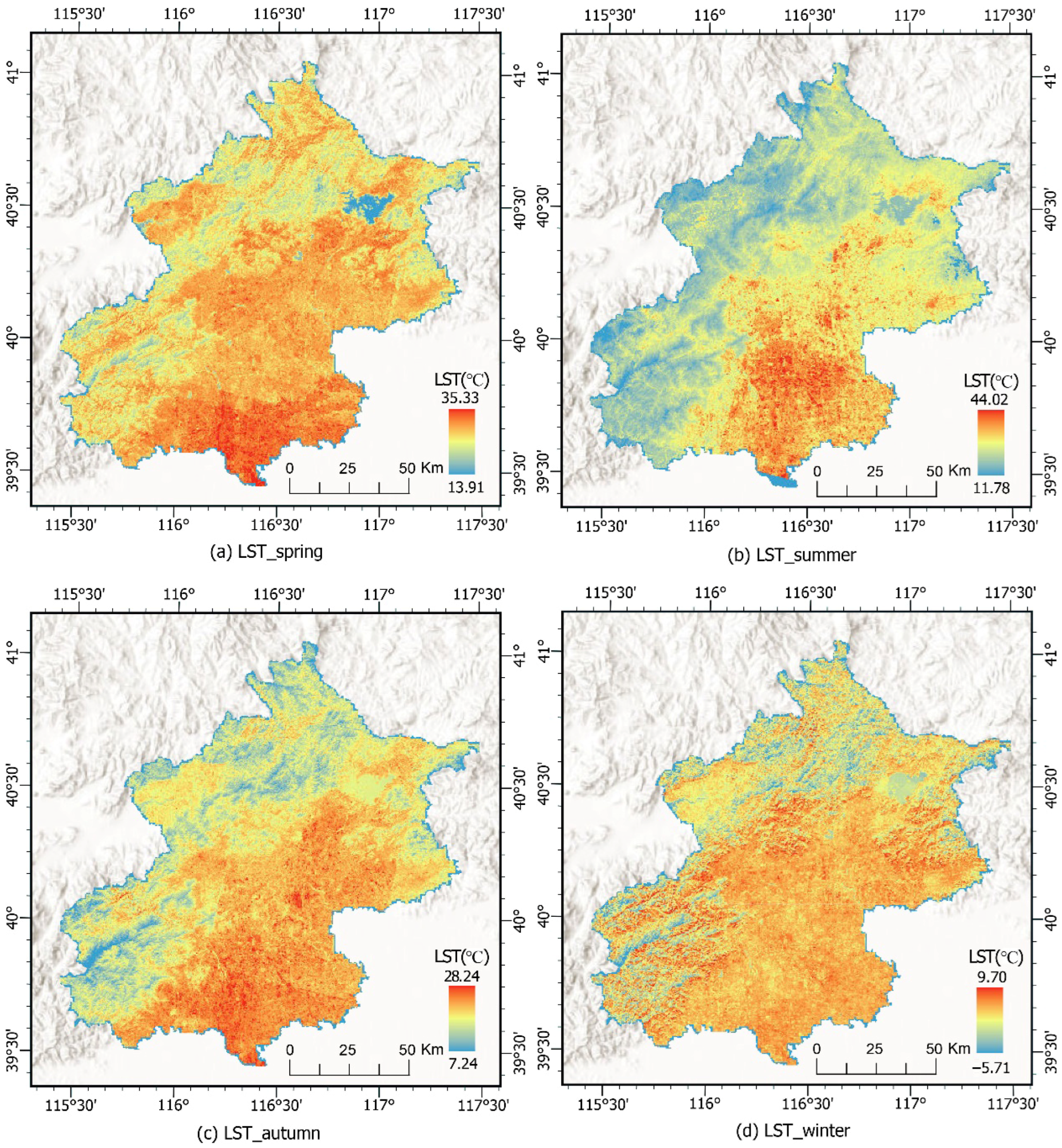
On the basis of Landsat 8 high-resolution remote sensing data, this study revealed that there were significant seasonal differences in LST across the study area (Table 3). The average temperature in summer was the highest (36.91 °C), and the average temperature in winter was the lowest (5.33 °C). The average temperature in spring (25.59 °C) was significantly higher than that in autumn (19.50 °C), which was consistent with the meteorological characteristics of rapid temperature recovery in spring in North China. The standard deviation of LST is greatest in summer (4.42 °C) and least in winter (2.05 °C), with spring and autumn being very similar at 2.47 °C and 2.50 °C, respectively. The results show that the urban surface energy budget in Beijing varies significantly by season and is closely related to the seasonal fluctuation in solar radiation intensity [28,36].
Figure 2 shows the spatial distribution of LST for the four seasons in Beijing. In spring, LST exhibited an uneven spatial distribution, and the areas with high temperature values were mainly concentrated in the central and southern regions (Figure 2a). Summer is marked by a pronounced rise in LST, with the most intense heat clustered in the urban core, establishing a distinct urban-rural thermal gradient (Figure 2b). LST in autumn and winter decreased rapidly, and the low-temperature areas were distributed mainly in the western and northern mountainous areas of Beijing.
Furthermore, considering the land use types in Figure 1, the high-value areas of LST in the four seasons in Beijing are mainly distributed in urban built-up areas and some areas with less vegetation coverage. In spring and autumn, the land surface temperature is relatively low in areas with high vegetation coverage (such as forests and grasslands), whereas the temperatures of artificially changed land types in built-up and cultivated areas are generally relatively high. Especially in summer, due to the high-temperature center formed by impervious surfaces and anthropogenic heat sources, the LST in the built-up area of southern Beijing is significantly higher than that in other areas [11,24]. In winter, the temperature in mountainous areas with high vegetation coverage decreases significantly, but the temperature in built-up areas is still relatively high, which reflects the heat island effect of urban heating and other factors to a certain extent.

3.2. Relative Impacts of Urban Features on LST

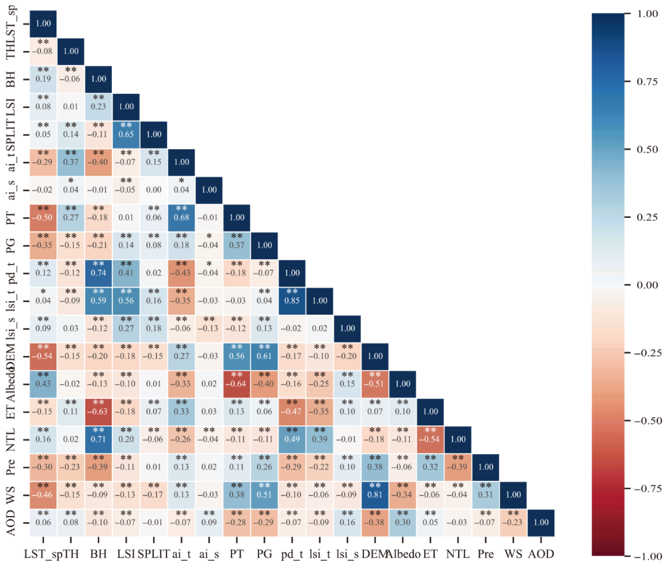
On the basis of the above understanding of the seasonal variation in LST in Beijing, we used the multicollinearity test method (Section 2.5) to screen out 18 variables from the urban landscape, natural environment, and human activity indicators according to VIF < 5 to analyze the impact mechanism on LST changes. First, the correlations with LST and seasonal differences among the 18 variables were analyzed (Figure 3). Although the correlation coefficients were numerically different, DEM, PT, PG, Pre, and WS were significantly negatively correlated with LST in any season, whereas albedo, lsi_s and AOD were significantly positively correlated with LST (Supplementary Figures S1–S3). For BH and ET, the response relationship to the LST in different seasons has contrasting characteristics. The correlations with LST and significances of traditional landscape pattern indices such as landscape shape index (LSI) and SPLIT are low.
In this study, the RF model was used to analyze the relative importance contribution to clarify the influence of different indicators on the seasonal variation in LST. Prior to this step, we first evaluated the RF model performance in the four seasons (Table 4). The results show that although the performance of the models is different between seasons, the R2 of each model is greater than 0.65, and the RMSE is less than 1.5, which achieves a good fitting effect. The relatively lower model performance in spring may be attributed to the region’s transient and non-stationary biophysical processes (e.g., rapid phenological changes and soil moisture variations), combined with the complex radiative properties of frequent dust aerosols, which together introduce greater unexplained variance.
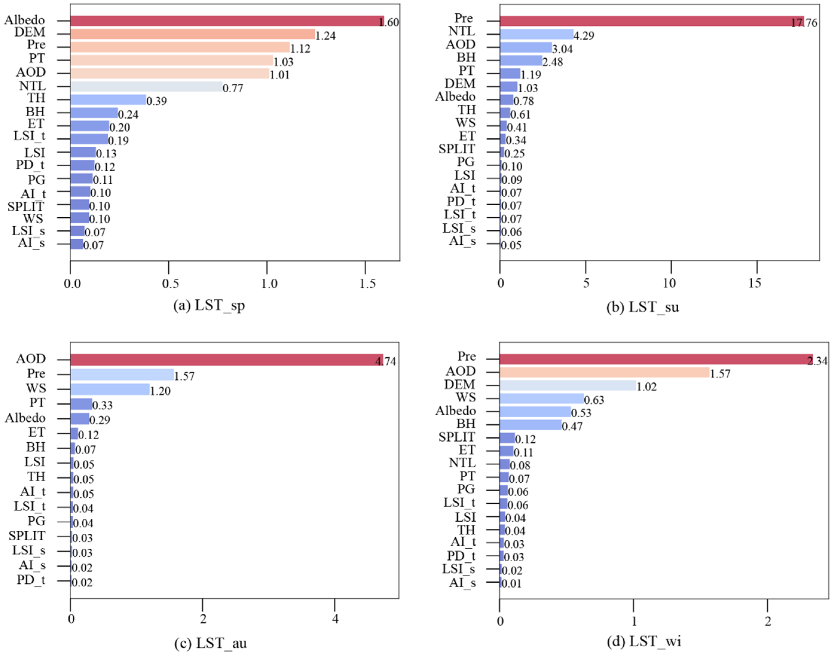
Overall, the importance of natural environmental factors (such as albedo, DEM, and Pre) and human activity factors (such as AOD and NTL) is high, whereas the importance of architectural and landscape pattern factors other than BH is low (Figure 4). A comparison of the importance contributions of the four seasons to LST reveals that the order of the variables significantly changes. The variable with the highest importance in summer and winter is Pre, especially in summer, with an importance value of 17.76 (Figure 4). The variables with the highest importance in spring and autumn are albedo and AOD, respectively. There are significant differences in the importance contributions of different variables to LST in each season. For example, the variable with the highest importance value in spring is albedo with 1.5, and the importance of the other top five variables also exceed 1. However, in autumn and winter, only the importance values of the top three variables exceed 1. These results suggest that the LST in different seasons is impacted complexly by many factors and that there may be synergistic effects among variables.
The quantitative single factor analysis revealed that the importance of the urban form and landscape index was less than that of meteorological, aerosol and human activities, and the response characteristics of LST to the different influencing factors were mostly nonlinear. Notably, albedo is of the highest importance only in spring, and LST shows an increasing trend with a slight increase in albedo, which indicates that the influence of albedo as a single factor on LST is not completely consistent with existing research and that this interaction or uncertainty needs to be verified.

3.3. Marginal Effects of the Main Indicators on LST

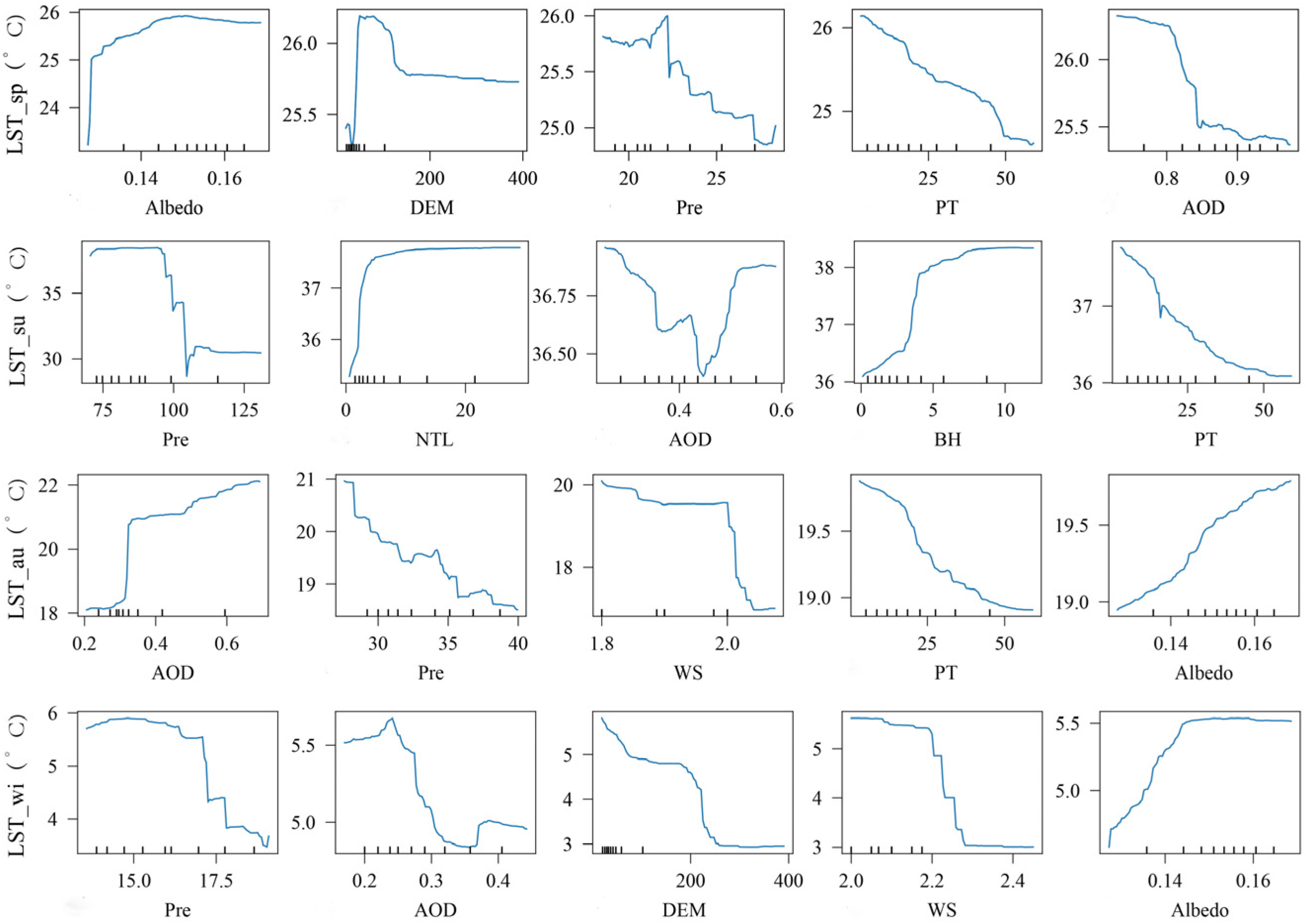
The marginal effect analysis keeps other variables unchanged to reveal how the target variable affects the prediction of LST. Based on the previous importance results, this section analyses the marginal effects of the top five variables in each season. As shown in Figure 5, the abscissa represents the value of the key independent variable index, and the ordinate reflects the degree of influence of the independent variable (i.e., partial dependence) on LST when other independent variables are controlled to be constant. Figure 5 offer a simplified visualization of the main trends, depicting the conditional expectation of LST by marginalizing over the distribution of other features. While this approach effectively illustrates the average marginal effect for interpretation, it may obscure local variations and uncertainties inherent in the underlying data.
The results show that the effects of different variables on LST are significantly different in the same season (Figure 5). In spring, for example, the partial dependence of LST on albedo first rapidly increases and then tends to be stable, with a demarcation point of approximately 0.14. With increasing values of PT and AOD, partial dependence of LST shows a continuous decline. Moreover, the effects of the same variable on LST also differs by season. In addition to the effects observed in spring, albedo and AOD have more consistent effects on LST in multiple seasons, whereas the effects of Pre and PT vary greatly across different seasons. Notably, the only indicators involved in all four seasons are AOD and Pre. Therefore, from the perspective of single factor changes, meteorological and atmospheric environmental factors have strong, stable impacts on temperature changes.
According to the response of LST to the influencing factors across seasons (Figure 5), the performances of the indices of vegetation coverage (PT), meteorological topography (WS, DEM) and human activity (NTL, BH) completely differ. First, PT shows a stable linear cooling trend for LST regardless of the season. The influences of WS and DEM on LST have certain threshold characteristics (Figure 5). LST first decreases and then maintains a constant value with increasing DEM, and the threshold of change is approximately 200 m. The influence of wind speed on LST is basically stable in the range of 0.2 m/s. Both NTL and BH promote rapid warming of LST and then gradually decrease in influence, which also reflects the close relationship between current urban thermal environment problems and the intensity of human activities [37,38].

3.4. Interaction Effects of the Main Indicators on LST

Table 5 shows the H-statistic and its corresponding combination and ranking. In this study, the H-statistics of all variable pairs in each season were calculated and the top five pairs were listed in Table 5. In the four seasons (Table 5), the factors with the greatest interaction effect on LST are Pre vs. AOD (spring), NTL vs. Pre (summer), WS vs. AOD (autumn) and Pre vs. AOD (winter). Correspondingly, their H-statistics are 0.12, 0.36, 0.37 and 0.33, respectively. From the perspective of seasonal differences, the bivariate interaction effect on LST in spring is the weakest, and the intensity of the bivariate interaction among the top five variables is between 0.12 and 0.06; the change in LST in winter may most be affected by interactions because the interaction values of the top five variables are all greater than 0.16, which is much greater than those in other seasons.
In this study, the effects of the interaction of different variables on LST were demonstrated via heatmaps and three-dimensional surface maps in spring (Figure 6). The results show that the influences of bivariate interactions on LST in summer, autumn and winter are similar (Supplementary Figures S4–S6). First, the bivariate interaction influence of Pre and DEM on LST is consistent. With increasing DEM (300 m), the surface temperature tends to decrease, and the cooling rate can reach 1.55 °C and 3.34 °C in spring and winter, respectively (Figure 6c and Figure S6d). It should be noted that spring and winter are the effects of the combination of DEM and PT, DEM and Pre, respectively. In addition, this does not mean that the increase in DEM continues to have the above cooling degree. The increase in precipitation often also has a significant cooling effect, and this cooling effect is exacerbated by a relatively high WS (Figures S5b and S6e). Second, NTL has weak interactions with other variables. In other words, LST did not significantly change with increasing or decreasing NTL (Figure 6d and Figure S4a).
Moreover, there are seasonal differences in the influences of different variable combinations on LST, among which PT is one of the most typical variables. In the spring in the study area, the combination of Pre and PT had a significant cooling effect (Figure 6e). However, in the interaction between Pre and PT in summer, only the increase in precipitation had a significant cooling effect, and there was no significant temperature change with increasing PT (Supplementary Figure S4d). In addition, the impacts of AOD on LST also differ. In spring, a relatively high AOD value is often accompanied by a decrease in surface temperature (Figure 6a), whereas in summer, a relatively high AOD only has a significant cooling effect after precipitation exceeds 100 mm (Supplementary Figure S4b). In autumn, when the threshold of AOD is less than 0.4, the temperature decreases with increasing precipitation. Considering that the composition of aerosols in different seasons is obviously different, the results of this study also indirectly indicate that, in addition to AOD, aerosol type may be a potential factor affecting the energy balance of the surface [21,37].

4. Discussion

4.1. The Effect of a Single Variable on LST

This study reveals the main driving factors of LST in different seasons in Beijing through variable importance ranking and partial dependence analysis. The influence of the natural environment, especially meteorological factors, on LST is very important. Pre can significantly increase atmospheric humidity and soil moisture and promote evaporation cooling in the short term, but the long-term impact of precipitation needs to be analyzed in combination with seasonal changes [39,40]. An appropriate wind speed may alleviate the heat island effect, but strong winds may also increase the diffusion of hot air and the range of influence of heat waves [41]. As shown in Figure 4, Pre has the most lasting effect on LST, with its importance values in summer, autumn and winter of 17.76, 1.57 and 2.34, respectively.
For the study area, the cooling effect caused by precipitation is achieved mainly through transpiration and a reduction in surface energy incidence. This phenomenon is particularly significant in summer because Beijing is dominated by convective rain in summer, and the heat in the boundary layer diffuses rapidly, which plays a central role in the urban thermal environment [39,40]. DEM and WS play prominent roles in temperature changes in winter and spring and autumn and winter, respectively (Figure 4). The monsoon climate and topographic distribution of Beijing can promote the transmission of cold air in winter and the deepening of the southeast monsoon in summer. In this study, in contrast with the warming effect of warm, humid air flow in summer, the sinking of cold air in autumn and winter can significantly reduce the temperature (Figure 5). In addition, the difference in mean LST between spring and autumn in Beijing is greater than 6 °C, indicating that although the solar radiation effects in the two seasons are similar, the differences in meteorology, underlying surface vegetation and human activities may affect LST.
This study uses the NTL and AOD to characterize human activities. The former can characterize the intensity of human activities, and high NTL values are often correlated with intensity of built-up areas, traffic, and industrial heat emissions [21,42,43]. The latter directly affects solar radiation and can also indirectly affect the surface energy balance by affecting the macro- and micro-characteristics of clouds [44,45,46]. We found that AOD has an important influence on LST in Beijing, which ranks in the top three influencing variables in summer, autumn, and winter. On the one hand, AOD can cool the surface through direct radiation effects and scattered solar radiation [19,36]. On the other hand, the warming effect of AOD on LST in autumn in this study indicates the influence of aerosol concentration and type on LST changes with region and season [47].
The characteristics of urban buildings and landscapes directly affect the urban wind field and heat island effects, which are classic indicators in urban research [42,48]. For example, high-density buildings hinder air circulation and aggravate the heat island effect, whereas high-rise buildings may reduce the local surface temperature through the shadow effect [17,18]. The landscape shape index and patch density of a city affect the heat exchange efficiency within the city and the local microclimate. The characteristics and proportion of vegetation have a significant impact on the urban thermal environment. Vegetation can reduce surface temperature by shading and transpiration and reduce heat absorption and accumulation. Relevant studies have shown that vegetation coverage is negatively correlated with urban heat island intensity and that the intensity of the urban heat island effect in China increases with a decrease in the difference between urban and rural vegetation coverage [17,23].

4.2. Interaction Effects of Various Variables on LST

According to the importance rankings, the change in LST is controlled by multiple variables (Figure 4), and the independent influence of key elements has obvious seasonal differences and nonlinear characteristics (Figure 5). Further quantitative analysis revealed that there is indeed a complex relationship between the variables (including Pre, AOD, DEM, PT, NTL, WS, and albedo) and LST (Figure 6, Supplementary Figures S4–S6). The interaction effect of AOD and DEM is dominant in spring (Figure 6). When AOD > 0.8, LST changes by 0.33–0.66 °C for every 100 m increase in DEM, which indicates that dust aerosols in spring in Beijing weaken solar radiation and the coupling effect with topography [21,28]. However, the influence of NTL on LST does not change significantly with changes in DEM (Figure 6d), which shows that human economic activities are not limited by terrain to a certain extent and can affect temperature changes over a wide range.
This study revealed that the influence degree and law of precipitation on the LST largely depend on the nature of the interaction factors. First, the interactions between Pre and DEM, WS and PT, which describe the natural environmental factors, show a superimposed cooling effect; that is, with increasing precipitation, DEM, WS and PT, LST rapidly decreases (Supplementary Figures S4–S6). On the one hand, both precipitation and wind speed are key variables that affect near-surface energy diffusion during convective weather processes. Therefore, increases in Pre and WS often indicate that the precipitation system is more powerful, so the cooling effect on LST is more significant. On the other hand, precipitation has a more obvious cooling effect on areas with higher altitudes and greater tree cover areas, which is closely related to the decrease in temperature itself with increasing altitude and the cooling effect of vegetation shading and transpiration [5,49]. Second, the interaction between Pre and AOD has grading characteristics. Specifically, low precipitation can promote a hygroscopic increase in aerosols, thereby synergistically reducing LST (Figure 6a and Figure S6a). When precipitation is high, the effect of aerosols is reduced by wet scavenging, thus high precipitation acts alone on LST (Supplementary Figures S4b and S5b). This understanding draws on the progress of aerosol-cloud-precipitation interactions, and it is necessary to recognize that the effects of different aerosol types are different [43,44,45,46].

4.3. Implications for Urban Planning and Management

The results of this study combined with the spatial distribution of land use types in the study area (Figure 1) reveal the significant differences in the regulatory effects of various factors on the LST of different land cover types. In fact, the main land use type in the central urban area of Beijing is built-up land, which is closely related to the increase in surface temperature. This is because impervious materials such as concrete and asphalt have low albedo (approximately 0.20) and high heat capacity characteristics. They absorb and store a large amount of solar radiation during the day and slowly release long waves at night to form a continuous heat island effect [50,51]. As shown in Figure 5, the LST increases by approximately 2 °C for every 10 m increase in building height. Especially in the context of high surface temperatures in summer, the superposition of human activities (such as heat release from air conditioners) may further aggravate the deterioration of the thermal environment.
In contrast, this study revealed that the regulatory effect of urban landscape morphology and surface vegetation coverage on LST was less than expected, but it still cannot be ignored (Figure 4). The regulation of vegetation on temperature is achieved mainly through biophysical processes: canopy transpiration reduces the proportion of sensible heat flux, and canopy shading reduces direct solar radiation to the surface and increases surface albedo. This study revealed that in areas with tree coverage greater than 30%, the summer LST was more than 10 °C lower than that in building-intensive areas (Figure 2). In addition, permanent water bodies reduce the surrounding microclimate temperature through the evaporative cooling effect in summer, but its influence range is limited (approximately 500 m in radius), and the local cooling effect may also occur in winter due to the increase in ice albedo [22,39].
The above mechanism shows that comprehensive consideration of the atmosphere, buildings and spatial configuration of vegetation/water is key for alleviating Beijing’s heat island effect [14,16]. Accordingly, this study also proposes strengthening the comprehensive environmental management and planning of megacities such as Beijing in three aspects. The first is to optimize urban planning, especially to fully consider the combination of building density, green space coverage, and other elements to avoid excessive concentration of high-density building areas. The second aspect to address is to pay attention to the impact of human activities, especially on the atmosphere. Previous studies have focused on the analysis of urban morphology and meteorological variables, often ignoring the change in surface energy balance caused by aerosols through absorption/scattering radiation. This study clearly reveals that a high AOD value (>0.20) is exponentially positively correlated with LST in autumn (the increase is close to 4 °C), and there is a “pollution-warming” positive feedback cycle. In addition, aerosols affect cloud microphysical processes, indirectly regulate precipitation and evapotranspiration, and should be included in assessments to analyze accurately the mechanisms determining the urban thermal environment. Third, due to the independent role of green space in regulating land surface temperature and its interaction with other factors, urban green spaces should be increased. Managers need to design green space types on this basis, such as considering the increase in cooling efficiency due to the combination of green space vegetation and precipitation. In the future, managers should try to build a coherent green space system to maximize this efficiency.

4.4. Limitations of the Study

This study provides insights into the driving factors for the seasonal variation in LST in Beijing, but some limitations should be recognized. First, we analyze the spatial resolution (1 km) of all variables [52,53,54]. Although it is suitable for the urban scale model, it may smooth the fine-scale heterogeneity in the urban structure, which may underestimate the role of variables such as building height. Similarly, the study period focused on the analysis of seasonal dynamics but limited the understanding of interannual variability and long-term trends. In addition, the use of nighttime light data as a proxy for human activities, although very common, may also not be able to directly capture anthropogenic heat flux, which indirectly answers its relatively low importance in this study.
Secondly, methodological limitations provide ideas for future research. Random forest models can capture complex nonlinear correlations, but potential biophysical mechanisms, such as the precise seasonal variation in aerosol effects, need to be further studied using atmospheric chemical models. In addition, although we use cross-validation, the inherent spatial autocorrelation of LST may lead to some performance index fitting preferences. Future research can benefit from the implementation of spatial cross-validation to obtain more robust model generalization estimation. Addressing these limitations through a combination of artificial intelligence and air quality models will further consolidate our understanding of the urban thermal environment.

5. Conclusions

This study analyzes the spatiotemporal dynamics of LST in Beijing across seasons using statistical methods and RF model, revealing the combined effects of urban landscape, meteorological, and atmospheric environment. Marked seasonal variations are observed: summer exhibits the highest mean LST and greatest variability, while winter shows the lowest. Although variability in spring and autumn is similar, the mean LST in spring (25.59 °C) is considerably higher than in autumn (19.50 °C). Moreover, the spatial variation in temperature is closely correlated with land use type. The areas with high LST values are concentrated in the central and southern urban areas, and the low-temperature areas are distributed mainly in the western and northern mountains and high vegetation coverage areas.
This study reveals that the individual influence on LST of meteorological factors, among which precipitation and aerosols are the most typical, is greater than that of urban factors. The cooling effect of precipitation on LST in Beijing is further amplified by relatively high wind speeds and high vegetation coverage. Our study quantifies the seasonally roles of aerosols (cooling in spring) and key nonlinear thresholds: a 50% increase in tree coverage cools LST by 1.5 °C, while a 10% increase in building height warms summer LST by 2 °C. These findings, along with strong factor interactions (e.g., precipitation-wind speed), provide a quantitative justification for integrating nonlinear responses into urban sustainability planning. Therefore, the interaction mechanism of weather–environment–building characteristics should be considered in future research to address the urban heat island problem.
The principal innovation of this work lies in its mechanistic insight: by employing a Random Forest framework, we move beyond identifying correlative drivers to quantitatively disentangle the complex nonlinear and interactive controls on LST, thereby revealing the dominant and seasonally modulated roles of aerosols and meteorological factors. Our findings call for integrated policies that not only regulate building density and height to mitigate warming but also explicitly leverage the cooling potential of urban greenery; simultaneously, continuous reduction in aerosols provides a key way to improve air quality and urban thermal environment.

Supplementary Materials

The following supporting information can be downloaded at: https://www.mdpi.com/article/10.3390/rs17233921/s1. Figure S1: Correlation analysis between land surface temperature (LST) and environmental variables in summer. */** represents passing the significance test; Figure S2: Correlation analysis between land surface temperature (LST) and environmental variables in autumn. */** represents passing the significance test; Figure S3: Correlation analysis between land surface temperature (LST) and environmental variables in winter. */** represents passing the significance test; Figure S4: Effect of bivariate interactions on land surface temperature (LST) in summer. (a) NTL and Pre interaction; (b) Pre and AOD interaction; (c) BH and Pre interaction; (d) PT and Pre interaction; (e) TH and Pre interaction; Figure S5: Effect of bivariate interactions on land surface temperature (LST) in autumn. (a) WS and AOD interaction; (b) Pre and AOD interaction; (c) Pre and WS interaction; (d) PT and WS interaction; (e) PT and AOD interaction; Figure S6: Effect of bivariate interactions on land surface temperature (LST) in winter. (a) Pre and AOD interaction; (b) Albedo and WS interaction; (c) DEM and Albedo interaction; (d) DEM and Pre interaction; (e) Pre and WS interaction.

Author Contributions

Conceptualization, S.Z. and H.F.; methodology, S.Z.; validation, Y.Y. and H.W.; formal analysis, H.W.; resources, H.F. and H.W.; data curation, Y.Y. and H.W.; writing—original draft preparation, S.Z.; writing—review and editing, H.F., J.Q. and X.L.; visualization, S.Z.; supervision, H.F.; project administration, H.F.; funding acquisition, H.F. All authors have read and agreed to the published version of the manuscript.

Funding

This study was supported by the National Natural Science Foundation of China (grant 42205178), the Fundamental Research Funds for the Central Universities (grant 2243100009), and the Tang Scholar Award.

Data Availability Statement

All data used in this study are listed in Section 2.2.

Acknowledgments

We thank all our colleagues who contributed to this work.

Conflicts of Interest

The authors declare that they have no known competing financial interests or personal relationships that could have appeared to influence the work reported in this paper.

References

  1. Abhijith, K.V.; Kumar, P.; Gallagher, J.; McNabola, A.; Baldauf, R.; Pilla, F.; Broderick, B.; Di Sabatino, S.; Pulvirenti, B. Air pollution abatement performances of green infrastructure in open road and built-up street canyon environments—A review. Atmos. Environ. 2017, 162, 71–86. [Google Scholar] [CrossRef]
  2. Wu, T.; Qiao, Z. Synergizing climate, energy, and air quality: Uncovering urban heat island, energy consumption, carbon emission, and air pollution nexus linkages. Environ. Impact Assess. Rev. 2026, 117, 108202. [Google Scholar] [CrossRef]
  3. Bokaie, M.; Zarkesh, M.K.; Arasteh, P.D.; Hosseini, A. Assessment of Urban Heat Island based on the relationship between land surface temperature and Land Use/Land Cover in Tehran. Sustain. Cities Soc. 2016, 23, 94–104. [Google Scholar] [CrossRef]
  4. Fahed, J.; Kinab, E.; Ginestet, S.; Adolphe, L. Impact of urban heat island mitigation measures on microclimate and pedestrian comfort in a dense urban district of Lebanon. Sustain. Cities Soc. 2020, 61, 102375. [Google Scholar] [CrossRef]
  5. Zeng, P.; Sun, F.; Liu, Y.; Tian, T.; Wu, J.; Dong, Q.; Peng, S.; Che, Y. The influence of the landscape pattern on the urban land surface temperature varies with the ratio of land components: Insights from 2D/3D building/vegetation metrics. Sustain. Cities Soc. 2022, 78, 103599. [Google Scholar] [CrossRef]
  6. Hatvani-Kovacs, G.; Belusko, M.; Skinner, N.; Pockett, J.; Boland, J. Heat stress risk and resilience in the urban environment. Sustain. Cities Soc. 2016, 26, 278–288. [Google Scholar] [CrossRef]
  7. Mallick, J.; Alqadhi, S. Explainable artificial intelligence models for proposing mitigation strategies to combat urbanization impact on land surface temperature dynamics in Saudi Arabia. Urban Clim. 2025, 59, 102259. [Google Scholar] [CrossRef]
  8. Jin, H.; Zhong, R.; Liu, M.; Ye, C.; Chen, X. Spatiotemporal distribution characteristics of PM2.5 concentration in China from 2000 to 2018 and its impact on population. J. Environ. Manag. 2022, 323, 116273. [Google Scholar] [CrossRef]
  9. Guo, F.; Hu, D.; Schlink, U. A new nonlinear method for downscaling land surface temperature by integrating guided and Gaussian filtering. Remote Sens. Environ. 2022, 271, 112915. [Google Scholar] [CrossRef]
  10. Kim, J.; Lee, D.-K.; Brown, R.D.; Kim, S.; Kim, J.-H.; Sung, S. The effect of extremely low sky view factor on land surface temperatures in urban residential areas. Sustain. Cities Soc. 2022, 80, 103799. [Google Scholar] [CrossRef]
  11. Xiang, Y.; Huang, C.; Huang, X.; Zhou, Z.; Wang, X. Seasonal variations of the dominant factors for spatial heterogeneity and time inconsistency of land surface temperature in an urban agglomeration of central China. Sustain. Cities Soc. 2021, 75, 103285. [Google Scholar] [CrossRef]
  12. Asgarian, A.; Amiri, B.J.; Sakieh, Y. Assessing the effect of green cover spatial patterns on urban land surface temperature using landscape metrics approach. Urban Ecosyst. 2015, 18, 209–222. [Google Scholar] [CrossRef]
  13. Su, H.; Han, G.; Li, L.; Qin, H. The impact of macro-scale urban form on land surface temperature: An empirical study based on climate zone, urban size and industrial structure in China. Sustain. Cities Soc. 2021, 74, 103217. [Google Scholar] [CrossRef]
  14. Peng, J.; Qiao, R.; Liu, Y.; Blaschke, T.; Li, S.; Wu, J.; Xu, Z.; Liu, Q. A wavelet coherence approach to prioritizing influencing factors of land surface temperature and associated research scales. Remote Sens. Environ. 2020, 246, 111866. [Google Scholar] [CrossRef]
  15. Wang, Q.; Wang, X.; Zhou, Y.; Liu, D.; Wang, H. The dominant factors and influence of urban characteristics on land surface temperature using random forest algorithm. Sustain. Cities Soc. 2022, 79, 103722. [Google Scholar] [CrossRef]
  16. Mo, Y.; Bao, Y.; Wang, Z.; Wei, W.; Chen, X. Spatial coupling relationship between architectural landscape characteristics and urban heat island in different urban functional zones. Build. Environ. 2024, 257, 111545. [Google Scholar] [CrossRef]
  17. Ren, Z.; Wang, C.; Guo, Y.; Hong, S.; Zhang, P.; Ma, Z.; Hong, W.; Wang, X.; Geng, R.; Meng, F. The cooling capacity of urban vegetation and its driving force under extreme hot weather: A comparative study between dry-hot and humid-hot cities. Build. Environ. 2024, 263, 111901. [Google Scholar] [CrossRef]
  18. Wang, C.; Ren, Z.; Guo, Y.; Zhang, P.; Hong, S.; Ma, Z.; Hong, W.; Wang, X. Assessing urban population exposure risk to extreme heat: Patterns, trends, and implications for climate resilience in China (2000–2020). Sustain. Cities Soc. 2024, 103, 105260. [Google Scholar] [CrossRef]
  19. Zheng, Z.; Zhao, L.; Oleson, K.W. Large model structural uncertainty in global projections of urban heat waves. Nat. Commun. 2021, 12, 3736. [Google Scholar] [CrossRef]
  20. Chen, M.; Dai, F.; Yang, B.; Zhu, S. Effects of urban green space morphological pattern on variation of PM2.5 concentration in the neighborhoods of five Chinese megacities. Build. Environ. 2019, 158, 1–15. [Google Scholar] [CrossRef]
  21. Ao, X.; Qian, J.; Lu, Y.; Yang, X. Mapping fine-scale anthropogenic heat flux in Shanghai by integrating multi-source geospatial big data using Cubist. Sustain. Cities Soc. 2024, 101, 105125. [Google Scholar] [CrossRef]
  22. An, Q.; Dong, Y.; Dong, W.; Xiao, S. Spatiotemporal dynamics and nonlinear landscape-driven mechanisms of urban heat islands in a winter city: A case study of Harbin, China. Sustain. Cities Soc. 2025, 133, 106842. [Google Scholar] [CrossRef]
  23. Hu, Y.F.; Dai, Z.X.; Guldmann, J.M. Modeling the impact of 2D/3D urban indicators on the urban heat island over different seasons: A boosted regression tree approach. J. Environ. Manag. 2020, 266, 110424. [Google Scholar] [CrossRef]
  24. Yang, X.; Leung, L.; Zhao, N.; Zhao, C.; Qian, Y.; Hu, K.; Liu, X.; Chen, B. Contribution of urbanization to the increase of extreme heat events in an urban agglomeration in east China. Geophys. Res. Lett. 2017, 44, 6940–6950. [Google Scholar] [CrossRef]
  25. Zhou, W.; Wang, J.; Cadenasso, M.L. Effects of the spatial configuration of trees on urban heat mitigation: A comparative study. Remote Sens. Environ. 2017, 195, 1–12. [Google Scholar] [CrossRef]
  26. Bai, K.; Li, K.; Ma, M.; Li, K.; Li, Z.; Guo, J.; Chang, N.-B.; Tan, Z.; Han, D. LGHAP: The Long-term Gap-free High-resolution Air Pollutant concentration dataset, derived via tensor-flow-based multimodal data fusion. Earth Syst. Sci. Data 2022, 14, 907–927. [Google Scholar] [CrossRef]
  27. Wang, Q.; Wang, X.; Meng, Y.; Zhou, Y.; Wang, H. Exploring the impact of urban features on the spatial variation of land surface temperature within the diurnal cycle. Sustain. Cities Soc. 2023, 91, 104432. [Google Scholar] [CrossRef]
  28. Liu, X.; Zhou, Y.; Yue, W.; Li, X.; Liu, Y.; Lu, D. Spatiotemporal patterns of summer urban heat island in Beijing, China using an improved land surface temperature. J. Clean. Prod. 2020, 257, 120529. [Google Scholar] [CrossRef]
  29. Yan, H.; Fan, S.; Guo, C.; Wu, F.; Zhang, N.; Dong, L. Assessing the effects of landscape design parameters on intra-urban air temperature variability: The case of Beijing, China. Build. Environ. 2014, 76, 44–53. [Google Scholar] [CrossRef]
  30. Roy, D.P.; Wulder, M.A.; Loveland, T.R.; Woodcock, C.E.; Allen, R.G.; Anderson, M.C.; Helder, D.; Irons, J.R.; Johnson, D.M.; Kennedy, R.; et al. Landsat-8: Science and product vision for terrestrial global change research. Remote Sens. Environ. 2014, 145, 154–172. [Google Scholar] [CrossRef]
  31. Han, D.; An, H.; Wang, F.; Xu, X.; Qiao, Z.; Wang, M.; Sui, X.; Liang, S.; Hou, X.; Cai, H.; et al. Understanding seasonal contributions of urban morphology to thermal environment based on boosted regression tree approach. Build. Environ. 2022, 226, 109770. [Google Scholar] [CrossRef]
  32. Daoud, J.I. Multicollinearity and regression analysis. J. Phys. Conf. Ser. 2017, 949, 012009. [Google Scholar] [CrossRef]
  33. Liu, X.; Zheng, L.; Wang, Y. Revealing the Roles of Climate, Urban Form, and Vegetation Greening in Shaping the Land Surface Temperature of Urban Agglomerations in the Yangtze River Economic Belt of China. J. Environ. Manag. 2025, 377, 124602. [Google Scholar] [CrossRef] [PubMed]
  34. Logan, T.M.; Zaitchik, B.; Guikema, S.; Nisbet, A. Night and day: The influence and relative importance of urban characteristics on remotely sensed land surface temperature. Remote Sens. Environ. 2020, 247, 111861. [Google Scholar] [CrossRef]
  35. Breiman, L. Random forests. Mach. Learn. 2001, 45, 5–32. [Google Scholar] [CrossRef]
  36. Chen, A.; Zhao, C.; Zhang, H.; Yang, Y.; Li, J. Surface albedo regulates aerosol direct climate effect. Nat. Commun. 2024, 15, 7816. [Google Scholar] [CrossRef] [PubMed]
  37. Manoli, G.; Fatichi, S.; Schläpfer, M.; Yu, K.; Crowther, T.W.; Meili, N.; Burlando, P.; Katul, G.G.; Bou-Zeid, E. Magnitude of urban heat islands largely explained by climate and population. Nature 2019, 573, 55–60. [Google Scholar] [CrossRef] [PubMed]
  38. Peng, S.; Piao, S.; Ciais, P.; Friedlingstein, P.; Ottle, C.; Bréon, F.-M.; Nan, H.; Zhou, L.; Myneni, R.B. Surface urban heat island across 419 global big cities. Environ. Sci. Technol. 2012, 46, 696–703. [Google Scholar] [CrossRef]
  39. Fan, Y.; Yang, Z.; Lo, M.H.; Hur, J.; Im, E.-S. Deciphering the capricious precipitation response: Irrigation impact in the North China Plain. Npj Clim. Atmos. Sci. 2025, 8, 211. [Google Scholar] [CrossRef]
  40. Li, C.; Gu, X.; Slater, L.J.; Liu, J.; Li, J.; Zhang, X.; Kong, D. Urbanization-induced increases in heavy precipitation are magnified by moist heatwaves in an urban agglomeration of East China. J. Clim. 2023, 36, 693–709. [Google Scholar] [CrossRef]
  41. Zong, L.; Liu, S.; Yang, Y.; Ren, G.; Yu, M.; Zhang, Y.; Li, Y. Synergistic influence of local climate zones and wind speeds on the urban heat island and heat waves in the megacity of Beijing, China. Front. Earth Sci. 2021, 9, 458. [Google Scholar] [CrossRef]
  42. He, W.; Li, X.-X.; Zhang, X.; Yin, T.; Norford, L.K.; Yuan, C. Estimation of anthropogenic heat from buildings based on various data sources in Singapore. Urban Clim. 2023, 49, 101434. [Google Scholar] [CrossRef]
  43. Sun, Y.; Wang, Y.; Zhao, C.; Zhou, Y.; Yang, Y.; Yang, X.; Fan, H.; Zhao, X.; Yang, J. Vertical Dependency of Aerosol Impacts on Local Scale Convective Precipitation. Geophys. Res. Lett. 2023, 50, e2022GL102186. [Google Scholar] [CrossRef]
  44. Zhang, J.; Guo, J.; Li, J.; Shao, J.; Tong, B.; Zhang, S. The Prestorm Environment and Prediction for Local- and Nonlocal-Scale Precipitation: Insights Gained from High-Resolution Radiosonde Measurements Across China. J. Geophys. Res. Atmos. 2022, 127, e2021JD036395. [Google Scholar] [CrossRef]
  45. Wang, S.; Zeng, X.; Huang, Y.; Li, X. Analysing urban local cold air dynamics and climate functional zones using interpretable machine learning: A case study of Tianhe district, Guangzhou. Sustain. Cities Soc. 2024, 114, 105731. [Google Scholar] [CrossRef]
  46. Yun, Y.; Zhang, D.-L.; Gao, W.; Yin, J.; Zhao, C.; Li, J.; Guo, J.; Liu, H. Spatiotemporal Variations of the Effects of Aerosols on Clouds and Precipitation in an Extreme-Rain-Producing MCS in South China. J. Geophys. Res. Atmos. 2024, 129, e2023JD040014. [Google Scholar] [CrossRef]
  47. Xiang, Y.; Ye, Y.; Peng, C.C.; Teng, M.J.; Zhou, Z.X. Seasonal variations for combined effects of landscape metrics on land surface temperature (LST) and aerosol optical depth (AOD). Ecol. Indic. 2022, 138, 108810. [Google Scholar] [CrossRef]
  48. Lauwaet, D.; Berckmans, J.; Hooyberghs, H.; Wouters, H.; Driesen, G.; Lefebre, F.; De Ridder, K. High-Resolution Modelling of the Urban Heat Island of 100 European Cities (2008–2017). Urban Clim. 2024, 54, 101850. [Google Scholar] [CrossRef]
  49. Walker, J.J.; de Beurs, K.M.; Wynne, R.H. Dryland vegetation phenology across an elevation gradient in Arizona, USA, inves-tigated with fused MODIS and Landsat data. Remote Sens. Environ. 2014, 144, 85–97. [Google Scholar] [CrossRef]
  50. Chang, W.; Guo, X. Disparities in the impact of urban heat island effect on particulate pollutants at different pollution stages—A case study of the “2 + 36” cities. Urban Clim. 2025, 59, 102273. [Google Scholar]
  51. Xin, C.; Qi, L.; Chu, H. Analysis of the midsummer local convection distribution and weather factors under the control of the Western Pacific subtropical high in the Yangtze Delta region of China. J. Meteorol. Environ. 2023, 39, 57–64. [Google Scholar]
  52. Wu, T.; Qiao, Z. Synergistic governance of urban heat islands, energy consumption, carbon emissions, and air pollution in China: Evidence from a spatial durbin model. Environ. Pollut. 2025, 372, 126025. [Google Scholar] [CrossRef] [PubMed]
  53. Li, X.; Zhou, Y.; Asrar, G.R.; Zhu, Z. Creating a seamless 1 km resolution daily land surface temperature dataset for urban and surrounding areas in the conterminous United States. Remote Sens. Environ. 2018, 206, 84–97. [Google Scholar] [CrossRef]
  54. Wang, Y.; Wang, H.; Yao, F.; Stouffs, R.; Wu, J. An integrated framework for jointly assessing spatiotemporal dynamics of surface urban heat island intensity and footprint: China, 2003–2020. Sustain. Cities Soc. 2024, 112, 105601. [Google Scholar] [CrossRef]
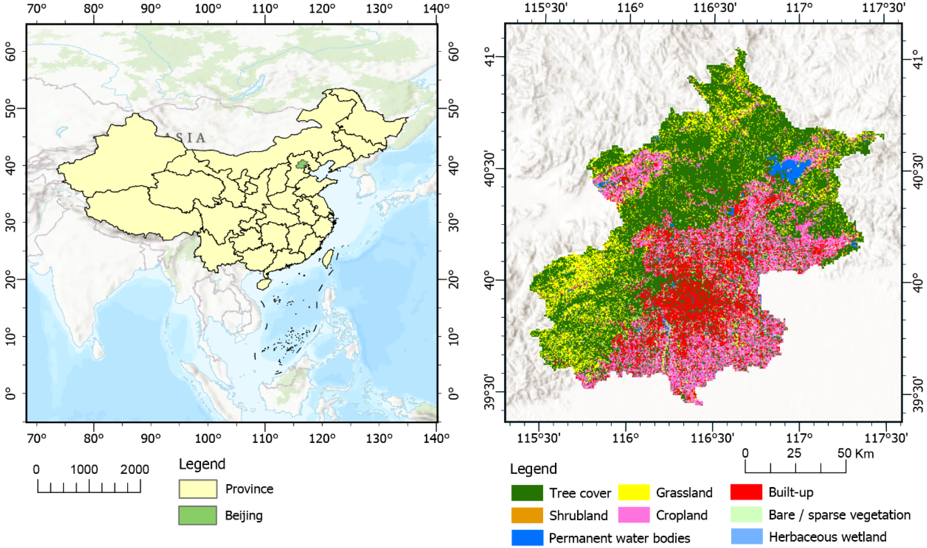
Figure 1. Location and land use types of the study area.
Remotesensing 17 03921 g001
Figure 2. Seasonal variation in LST in the study area. Spring, summer, autumn, and winter are March–May, June–August, September–November and December–February, respectively. The boundary of the study area is blue lines.
Remotesensing 17 03921 g002
Figure 3. Correlation analysis between LST and environmental variables in spring. */** represents passing the significance test.
Remotesensing 17 03921 g003
Figure 4. Ranking the importance of impact factors, (ad) represent spring, summer, autumn, and winter, respectively. These abbreviated variables and their corresponding meanings in the ordinate have been listed in Table 2.
Remotesensing 17 03921 g004
Figure 5. Partial dependence of LST on important input variables. Lines 1 to 4 represent the results for spring, summer, autumn and winter, respectively.
Remotesensing 17 03921 g005
Figure 6. Effect of bivariate interactions on LST in spring. (a) Pre and AOD interaction; (b) DEM and AOD interaction; (c) PT and DEM interaction; (d) DEM and NTL interaction; (e) PT and Pre interaction.
Remotesensing 17 03921 g006
Table 1. The key dataset in this study.
DataSpatial ResolutionURL
LST/Albedo30 mhttp://earthexplorer.usgs.gov (accessed on 27 July 2025)
ESA World Cover 202010 mhttps://worldcover2020.esa.int/ (accessed on 6 July 2025)
Aerosol1 kmhttps://doi.org/10.5281/zenodo.5652257 (accessed on 29 June 2025)
DEM30 mhttps://earthexplorer.usgs.gov/ (accessed on 29 June 2025)
NTL500 mhttps://www.ngdc.noaa.gov/eog/viirs (accessed on 30 July 2025)
GFCH30 mhttps://glad.umd.edu/dataset/gedi (accessed on 24 November 2025)
Evapotranspiration500 mhttps://search.earthdata.nasa.gov/search?q=MOD16A2 (accessed on 13 July 2025)
Precipitation0.1°https://cds.climate.copernicus.eu/datasets (accessed on 14 June 2025)
Table 2. The classification, abbreviations, and descriptions of the influencing variables.
Category of VariablesVariableMeaning of Variable
Buildings and landscapeBHAverage height of each building
SPLITLandscape type separation index
LSILandscape shape index reflects patch shape complexity
lsi_tLandscape shape index of trees
lsi_sLandscape shape index of shrubs
pd_tPatch density of trees
ai_tLandscape aggregation index of trees
ai_sLandscape aggregation index of shrubs
Vegetation indexTHAverage height of trees
PTPercentage of tree area
PGPercentage of grassland area
Natural environmentalDEMAverage elevation of the grid
AlbedoAverage surface albedo value
ETMean value of evapotranspiration
PreMean value of precipitation
WSMean value of wind speed
Human activityNTLMean value of NTL for the detection of human activity
AODAverage aerosol optical depth represents the atmospheric pollution
Table 3. The seasonal variation characteristics of LST in Beijing.
MetricsLST_sp (°C)LST_su (°C)LST_au (°C)LST_wi (°C)
Mean25.5936.9119.505.33
Standard Deviation2.474.422.502.05
Min13.9111.787.12−5.71
Max35.3344.0228.249.70
Table 4. The performance of the random forest model in different seasons. R2 represents the degree of fit, and RMSE represents the root mean square error.
SeasonR2RMSE
Spring0.671.44
Summer0.851.90
Autumn0.890.84
Winter0.850.86
Table 5. Variable combinations and their interaction effect value.
Dependent VariableRankCharacteristic Quantity GroupH-Statistic
LST_sp1Pre vs. AOD0.12
2DEM vs. AOD0.10
3PT vs. DEM0.07
4DEM vs. NTL0.07
5PT vs. Pre0.06
LST_su1NTL vs. Pre0.36
2Pre vs. AOD0.26
3BH vs. Pre0.17
4PT vs. Pre0.11
5TH vs. Pre0.09
LST_au1WS vs. AOD0.37
2Pre vs. AOD0.18
3Pre vs. WS0.09
4PT vs. WS0.06
5PT vs. AOD0.05
LST_wi1Pre vs. AOD0.33
2Albedo vs. WS0.21
3DEM vs. Albedo0.21
4DEM vs. Pre0.19
5Pre vs. WS0.16
Disclaimer/Publisher’s Note: The statements, opinions and data contained in all publications are solely those of the individual author(s) and contributor(s) and not of MDPI and/or the editor(s). MDPI and/or the editor(s) disclaim responsibility for any injury to people or property resulting from any ideas, methods, instructions or products referred to in the content.