Article

Benchmarking Elevation Plus Land Surface Parameters Finds FathomDEM and Copernicus DEM Win as Best Global DEMs

by
Peter L. Guth
1,*,
Sebastiano Trevisani
2,
Carlos H. Grohmann
3,
John B. Lindsay
4 and
Hannes I. Reuter
5
1
Independent Researcher, Annapolis, MD 21401, USA
2
Dipartimento di Culture del Progetto, University Iuav of Venice, Terese-Dorsoduro 2206, 30123 Venice, Italy
3
Institute of Astronomy, Geophysics and Atmospheric Sciences, Universidade de São Paulo, São Paulo 05508-090, Brazil
4
Department of Geography, Environment & Geomatics, The University of Guelph, Guelph, ON N1G 2W1, Canada
5
Independent Researcher, 54294 Trier, Germany
*
Author to whom correspondence should be addressed.
Remote Sens. 2025, 17(23), 3919; https://doi.org/10.3390/rs17233919
Submission received: 9 October 2025 / Revised: 21 November 2025 / Accepted: 27 November 2025 / Published: 3 December 2025
(This article belongs to the Section Environmental Remote Sensing)

Highlights

What are the main findings?
  • Digital elevation models with one-arc-second are still the best free scale available globally. When compared to a lidar-derived reference digital terrain model, FathomDEM consistently performs best but has a restrictive license. The Copernicus DEM is the best free option, with the ALOS AW3D30 only in rugged and steep mountainous areas. We also evaluated FABDEM and GEDTM v1.2.
  • The capability of global DEM to represent land surface parameters, such as slope, curvatures, and roughness changes in relation to land cover and morphology. Parameters computed with the second order partial derivatives show a range of correspondence, and those computed with third order partial derivatives show extremely low correspondence.
What is the implication of the main finding?
  • The procedures for creating a bare earth digital elevation from a digital surface model are a black box that can hallucinate, and the results must be checked carefully. The creators should check derived land surface parameters as well as the raw elevation values, as a good digital surface model can be better than a poor digital terrain model.
  • Geomorphometry workers must carefully assess the land surface parameters they use. First derivative parameters perform best; second derivative parameters, like curvature, vary in their signal-to-noise ratio; the third derivative parameters, like change of curvature, might be all noise.

Abstract

We evaluated six global digital elevation DEMs at 1-arc-sec resolution: CopDEM and AW3D30, which are digital surface models (DSMs), and EDTM, GEDTM, FABDEM, and FathomDEM, which are digital terrain models (DTMs). We compared them to reference DTMs created by mean aggregation from 1–2 m lidar-derived DTMs from national mapping agencies, using 1510 approximately 10 × 10 km test tiles from the United States and western Europe. Our criteria used the grids for elevation and derived land surface parameters (LSPs), including characteristics of the difference distributions and the fraction unexplained variance derived from grid correlations. The best DEM depends on the LSP used and the characteristics of the test tile, especially average slope, barrenness, and forest coverage. FathomDEM emerged as the best among the DEMs, with CopDEM the best overall for the DEMs with unrestricted licenses. GEDTM performed poorly. This is especially important for LSPs like curvature measures, which require higher-order partial derivatives for computation, and which should be used very cautiously.

1. Introduction

Digital elevation models (DEMs) provide one of the fundamental building blocks for scientific, commercial, military, and recreational users. Despite the growing availability of high-resolution DEMs with about 1 m spatial resolution, for much of the world, only one-arc-second DEMs are freely available for users who cannot afford higher-resolution commercial data. In addition, for many uses, including orthorectification of satellite imagery or regional studies, one-arc-second DEMs provide adequate resolution, lower storage costs, and much faster processing because they have about one nine-hundredth the number of elevation pixels compared to a one-meter DEM.
DEMs can be digital surface models (DSMs), the first surface seen by the sensor, or bare-earth digital terrain models (DTMs), the surface of the ground after removal of vegetation, buildings, and other anthropogenic features [1]. High-resolution current lidar sensors achieve a high point density and can create DTMs by removing vegetation and identifying the tops of buildings, but the current optical and radar satellite sensors used to create global DEMs can only achieve limited penetration of the vegetation and can only create DSMs. This has led to a number of efforts to use ancillary data sets, including vegetation estimates, to edit DSMs to create a global DTM starting with Bare-Earth SRTM [2], MERIT [3], and FABDEM [4].

1.1. Accuracy Assessments of DEMs

Comparisons of DEM accuracy have used several strategies, based on the map accuracy standards applied to topographic maps. These include using a small number of accurate control points, using points collected along the ground path of laser altimeters, using a lidar point cloud, and comparing every point in the DEM to another DEM with higher accuracy. A one-arc-second DEM for a 10 × 10 km area will have about 140,000 elevations, varying with latitude. Most accuracy assessments focus only on elevation, and not the derived land surface parameters (LSPs), which are frequently the most important product for DEM users.
Probably the most common method has been applying metrics like RMSE, MAE, or LE90 to a relatively small number of control points, which can be national mapping agency benchmarks, GNSS survey points, or the control points used by contractors performing lidar surveys. Recently, the GEDTM DEM  [5] used GNSS survey points [6,7], which have at most 25 points in a 10 × 10 km tiles and globally only 23,134 GPS stations to cover 1.5 million tiles. Contractor control points used for lidar projects along the US coast had at most 19 points per tile [8,9]. The commercial AIRBUS GCP database has a point for every 2 km2, or 50 points per 10 × 10 km tile [10]. Besides the relatively small number of control points, their distribution can concentrate on relatively flat positions with land cover providing a good view of the sky.
DEM assessment can utilize satellite laser altimeters like ICESat-2 or GEDI [11], which provide along-track elevation profiles, both for the ground surface and the top of the vegetation canopy [12,13]. Even after seven years of data collection, ICESat-2 has returns in fewer than 10% of 30 m pixels. This number varies with the overlap of the area with the satellite ground tracks, the weather during satellite overpasses every three months, and whether the user chooses ATL03 raw photon or ATL08 binned terrain data. This estimate agrees with the suggestion that ICESat-2 could only support creation of a DEM at 90 m resolution [14], which has only one-ninth the number of elevation pixels of the 30 m DEMs. The greater density of points in the along-track direction means that neighborhood elevations might vary in quality, particularly critical for operations like slope computation. The availability of two web platforms, SlideRule [15] and OpenAltimetry [16], for easy download of this data encourages its use.
The point clouds from airborne lidar provide another mechanism for comparing DEMs. These have much higher point densities compared to the satellite altimeters and form the basis for the high-resolution DTMs being produced and freely distributed for Western Europe and North America. The volume of data required for these analyses, at least an order of magnitude greater than the DEMs derived from them, limits their application. One of the first comparisons of the CopDEM combined ICESat-2 and airborne lidar [17] for a limited number of test areas. The point cloud will typically have thousands to tens of thousands of elevation samples for every pixel in a one-arc-second DEM.
The Digital Elevation Model Intercomparison eXercise (DEMIX) had two innovations: using the entire grid, and evaluating both the DEM and LSPs derived from it [18].

1.2. Rationale for This Work

The appearance of two new edited one-arc-second DTMs, FathomDEM [19,20,21] and GEDTM [5,22,23,24], encouraged us to repeat and extend the earlier comparisons [18,25] of DEMs with the latest edited DTMs. Although GEDTM is advertised as having one-arc-second spacing, its original releases [22,23] in fact had 0.9 arc-second spacing and did not align with any of the one-arc-second DEMs (Figure 1). The smaller pixel spacing required GEDTM to interpolate for their final DEM, and the smaller pixel size changes LSP parameters, such as slope, which will be steeper. GEDTM has no license restrictions that have led to significant downloads, and users should know how they compare with the alternative DEMs, both free and with restrictive licenses like FathomDEM.
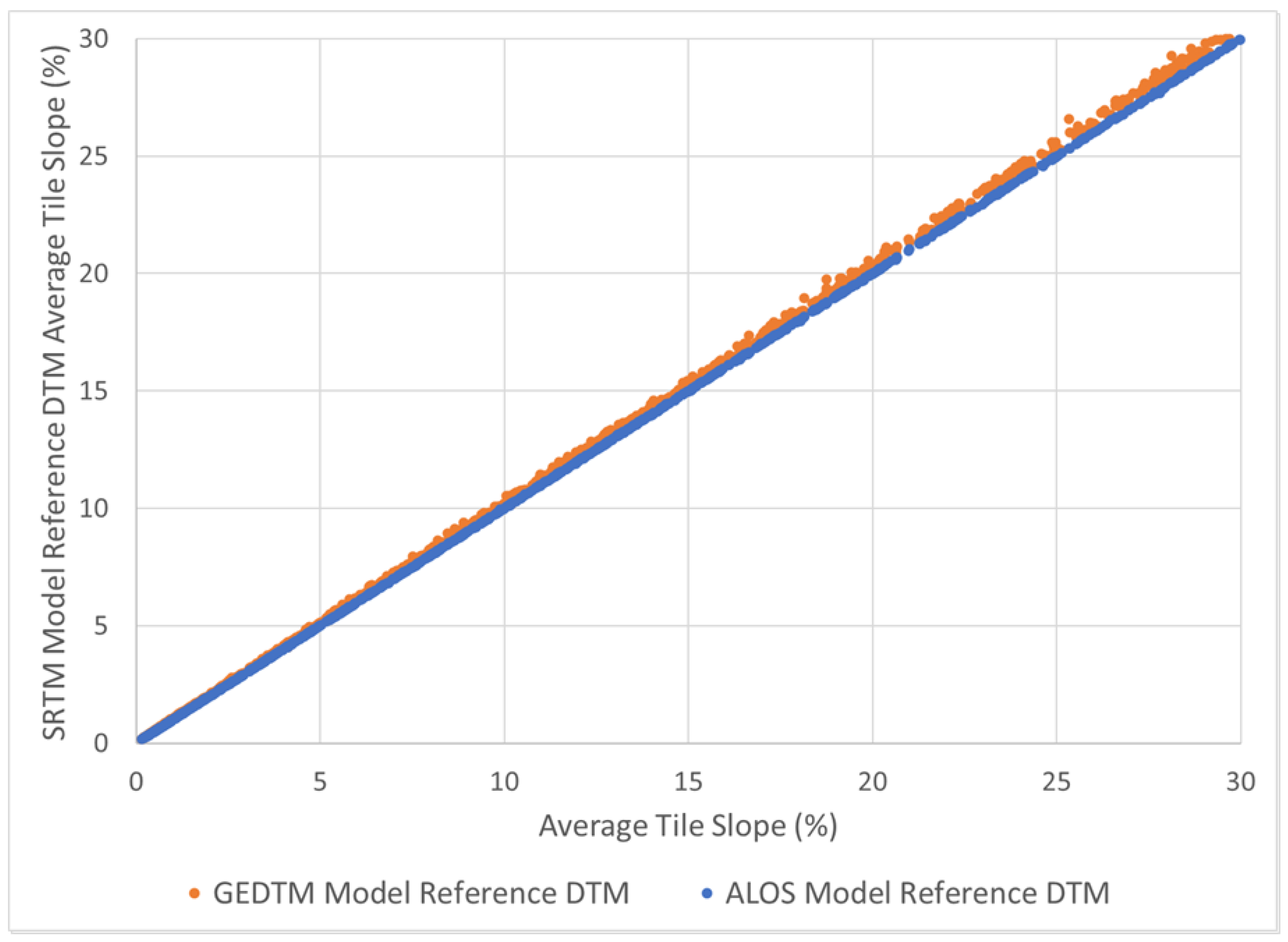
The one-arc-second DEMs use two different geometric models, with a 1/2 pixel difference in pixel positioning. While this means that pixel values cannot be compared in DEMs with different geometries without interpolating in one of the grids, this does not greatly affect the statistical properties of the DEMs (Figure 2) as long as the pixel spacing remains the same. Users who would like to see how the 0.9 arc-second GEDTM affects the results can use version 3.5 of the DEMIX database, which includes three versions of GEDTM [26].
A fundamental assumption behind DEMIX work has been to only compare DEMs with the same pixel spacing and geometric model to avoid introducing additional differences resulting from reinterpolation. We deal with the different pixel models by using one test DEM with that pixel geometry model, and then aggregate the high-resolution DTM to match the pixels in the model to create our reference DTM. We average all pixels in the high-resolution DTM that map to the pixel in the one-arc-second test DEM and the new reference DTM. For high latitude locations where ALOS and COPDEM change the longitudinal spacing, we make additional reference DTMs.Creating reference DTMs is the most labor-intensive and time-consuming step in comparing DEMs. Faced with the need to create 0.9 arc second reference DTMs to fairly evaluate GEDTM before its authors released a true 1-arc-sec version, we reevaluated and improved the entire processing pipeline. The biggest change was a switch to UTM-based test tiles from geographic tiles [27]. While the creators of the GEDTM dataset have now produced a 1-arc-sec version, we retain our new procedure for its improvements and greater efficiency.

1.3. UTM-Based DEMIX Tiles

The original DEMIX tiles [27] used geometric coordinates chosen so tiles were about 10 × 10 km in size. Due to the convergence of the meridians, the tiles changed in size with latitude, and the longitudinal spacing of the tiles changed at several latitudes to minimize the changes in overall tile size, similar to the changes in spacing for DEMs like DTED or Copernicus.
The source DEMs to create reference data all use tiles based on UTM, or a geometrically similar national projected coordinate system. Tile boundaries in national data sets are either based on uniformly sized projected grid coordinates or match the map quadrangle boundaries of the national topographic maps. DTMs from USGS have 10 × 10 km tiles, but to fill a single geographic DEMIX tile almost always requires four UTM tiles because the grids do not coincide. Using the tiles downloaded from USGS and other national providers directly achieves all the goals of the DEMIX tiles: test areas of nearly constant size, tile names that uniquely point to the location, and a uniform sampling scheme. Tiles cannot easily merge at the boundaries of UTM zones, but neither can the national mapping agency’s high-resolution 1 m DEMs, and tiles can be extended a short distance across the UTM zone boundary. This is conceptually similar to the tile geometry and names for Sentinel-2 satellite imagery. For countries that do not provide 10 km tiles, such as Denmark, Switzerland, and the United Kingdom, multiple tiles can be merged to obtain a 10 × 10 km tile in a relatively simple process based on the file names.
Countries that distribute their DEMs to match national map quadrangles, such as Mexico, the Netherlands, and Spain, either already have tiles approximately 10 × 10 km or allow four DEM tiles to be merged to create such tiles. The actual tile sizes vary with latitude, but for statistical purposes, we view all of these as similar to the 10 × 10 km goal, which also varied by latitude for the geographic DEMIX tiles. We name the tiles for either the projected coordinates of the SW corner or the national map quadrangle name; the naming convention differs by country. The latitude and longitude of the tile’s centroid, included in all of our databases, provide an easy way to locate tiles, and we have code to create the bounding boxes for all tiles.
We restrict our reference areas to those meeting the following conditions:
  • Online government portal to download DTMs in Geotiff format.
  • Grid spacing of 2 m or smaller. If the country has several resolutions, such as Switzerland, we use the larger grid spacing as aggregation to one-arc-second will not benefit from the smaller grid spacing.
  • Vertical datum shifts to EGM2008 from the original datum supported by GDAL [28]. If this is not possible, we can use the DEM only for LSPs that do not depend on absolute elevation values.
  • Availability of tiles approximately 10 × 10 km, or under 10 × 10 km that can be merged into tiles of approximately 10 × 10 km. This rules out huge, multi-GB files. While we could extract tiles from such files, it would not add much to the diversity of test areas.
  • Elevations in floating point meters with resolution to at least a decimeter.
Table 1 summarizes the characteristics of the governmental mapping data sets that meet our criteria. The Geotiff metadata in the file headers for all these DTMs contain the horizontal projection, but none have the vertical datum, which we have to add manually. The national mapping agencies also vary in their inclusion of the DTM’s date in the file name. While all of the national mapping agencies have metadata about their data on the websites, when users are dealing with thousands of files it would preferable for the key metadata about the DEM to be either included in the Geotiff header or encoded in the file name.
Adding a new national data set requires about a half dozen lines of code [42] to create the tile name from the downloaded file names, and instructing GDAL [28] how to perform the horizontal and vertical datum shifts. We also have code to help sort a large number of small 1 × 1 km tiles into 10 × 10 km directories.
For simplicity in comparing the two tile types, we will use labels GEO and UTM, recognizing that some of the UTM tiles actually use a slightly different national grid. The UTM and national grids would have pixels at different locations, and likely a slight rotation, but when aggregated to 1-arc-sec reference grids, they would be very similar. While the test tile boundaries are defined by projected coordinates, we aggregate to geographical grids to create test DTMs to match the global DEMs.

2. Materials and Methods

This is the third paper contributing to the DEMIX comparison. Each paper improved the method, increased and diversified the characteristics of the test areas, and added new global 1-arc-sec DEMs.

2.1. Key Definitions

The methodology uses the following definitions:
  • Criterion: LSP used to compare a test and reference DEM.
  • Evaluation: numerical result of a comparison between a test and reference DEM.
  • Reference DTM: our best estimate of the true bare earth surface, created from a high-resolution DTM to match the pixel geometry and spacing of the test DEM.
  • Test DEM: one of the group of 1-arc-sec DEMs being compared. The only changes to the test DEMs are a vertical datum shift if required to move to EGM2008.

2.2. Summary of Current Procedure

We highlight our current method, modified from [25], which was in turn modified from [18].
  • Test DEMs are 1-arc-sec DEMs, WGS84 horizontal datum. We shift AW3D30 to the EGM2008 vertical datum used by the others. Some earlier versions of GEDTM have 0.9-arc-second spacing, which required special creation of references DTMs at that pixel size for version 3.5 of our database [26].
  • Download high-resolution DTMs from the governmental mapping agency. Table 1 shows the national data sets we have used. Our primary US data source [41] delivers 10 × 10 km tiles with a very small boundary buffer. Due to the large size of the US and the wide range of landscapes, we feel it provides a good sample of Earth’s topography, but the additional countries in Mexico and Western Europe extend our sample.
  • Create landcover grid from 10 m resolution ESA World Cover 2021 [43] for each test tile. This replaces the 100 m Copernicus Global Land Cover 100 m [44] used previously.
  • Use GDAL [28] to shift the source DTMs from the local projection and datum to the WGS84 ellipsoid and EGM2008 vertical datum, shifting to a UTM projection for countries that use a national projection. This results in small shifts both horizontally and vertically, which are much smaller than one arc second.
  • For each test tile, create two reference DTMs (1-arc-sec SRTM geometry and 1-arc-sec ALOS geometry), and when required at higher latitudes, reference DTMs with increased longitudinal spacing. We use mean aggregation into the rectangular pixels in the geographic reference DTMs for the two geometries. The geographic grid will have small triangular missing data regions on each edge of the DEM, whose size varies with distance from the central meridian of the UTM zone. These missing data regions are ignored for the computations to follow, and have negligible effect on the statistics.
  • Use a number of land surface parameters (LSPs) as analysis criteria, computed with open source programs.
  • For each criterion, compute the Pearson correlation coefficient (r2) between the LSP derived from the test DEM with the appropriate reference DEM, with pixel centroids at the same geographic location.
  • Mask out water using the landcover [43].
  • Compute the fraction of unexplained variance (FUV), which is (1 − r2). This ranges from 0 (best) to 1 (worst).
  • Create a database by computing FUV statistics for the LSP criteria for each test tile.
  • Compute databases with FUV statistics for the partial derivatives and curvature measures [45,46].
  • Create a database for the different distributions used in the first DEMIX work [18].
  • The resulting databases have a row for each DEMIX tile and criterion, and a column for each test DEM.
  • Compute tile characteristics from the SRTM geometric model one-arc-second reference DTM, and the 10 m landcover, and merge them into the other databases.
  • All computations were done with MICRODEM [42,47].

2.3. Changes to Method

We made the following changes to the previous methodology [25], summarized in Table 2:
  • We have slightly changed the selection of FUV criteria used. The actual criteria are less important than the patterns. All selected criteria are now computed with free, open-source software.
  • We use lsp-calculator [45,46] to compute two new database tables, with the partial derivatives used to compute slope and curvature, and the full set of curvatures [48].
  • We do not compute or use the per-pixel raster classification or vector comparison criteria, which we find redundant as they follow the same trends as the grid FUV criteria.
  • We do not consider SRTM, ASTER GDEM, NASADEM, and 1-arc-sec TANDEM-X. Previous work [18,25] clearly shows these datasets should be retired. Figure 3 shows that compared to CopDEM, only one of these is ever superior and only in some low-slope, forested tiles.
  • All tiles have at least 35,000 valid points after water masking. The number varies because the UTM tiles have variable numbers of points due to irregular boundaries along the coast, political boundaries, or mapping project edges.
  • We did not analyze coastal test DEMs. There have been a few recent changes in the edited coastal DTMs, and the conclusion that low-relief coastal DEMs at the one-arc-second scale do not perform well remains valid [25].
  • We have slightly fewer test tiles after changing from GEO to UTM tiles, but more test areas. We removed some areas that did not meet our improved requirements, and some coastal areas, because of their demonstrated poor performance. When we added additional tiles, we opted for more test areas with fewer tiles each to add more geographical variety.
Table 2. Evolution of the DEMIX database.
Bielski et al., 2024 [18]Guth et al., 2024 [25] This Work
Database versionv2 [50]v3 [49]v3.5 [26]v4 [51]
Test areas24124140155
Test tiles236346213811510
Tile geometryGeographic [27]Geographic [27]National DEM projection (Table 1)National DEM projection (Table 1)
Global DEMsALOS, ASTER, CopDEM, FABDEM, NASADEM, SRTMALOS, ASTER, CopDEM, FABDEM, NASADEM, SRTM, TanDEM-XALOS, CopDEM, FABDEM, FATHOM, EDTM, 3 GEDTMALOS, CopDEM, FABDEM, FATHOM, GEDTM
Coastal DEMs Coastal; Delta; Diluvium
Difference distribution criteriaElevation; slope; roughness; 5 measures eachElevation; slope; roughness; 5 measures eachElevation; slope; roughness; 5 measures eachElevation; slope; roughness; 5 measures each
Mixed FUV criteria 1715 (open source software)15 (open source software)
Pixel classification criteria 8
Vector match criteria 2
Partial derivative FUV criteria 1111
Curvature FUV criteria 2828

2.4. Test Areas

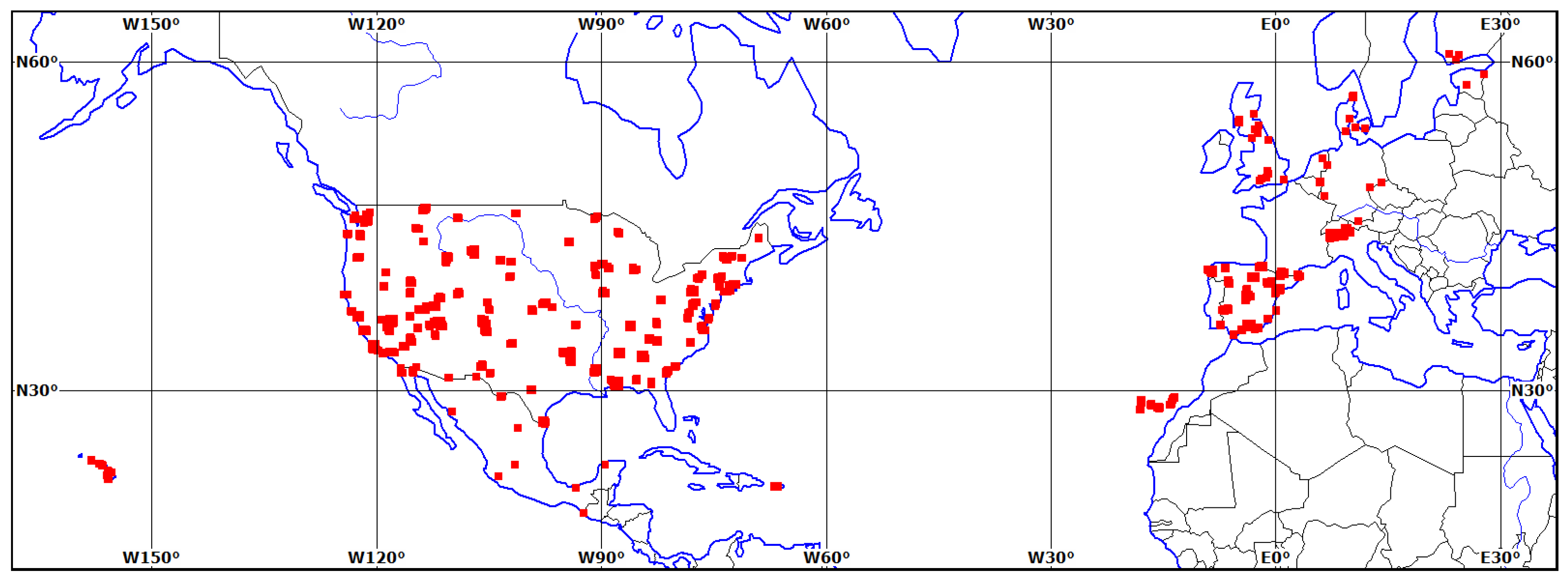
Figure 4 shows the test areas. There are more distinct areas (154), but fewer tiles (1510) than in the last DEMIX work [25]. That work overemphasized coastal tiles, which perform poorly for all the global DEMs, and included a large number of tiles that do not meet our improved selection criteria. We are confident that the current test tiles provide a more balanced sampling in terms of morphology and landcover characteristics than the earlier work.
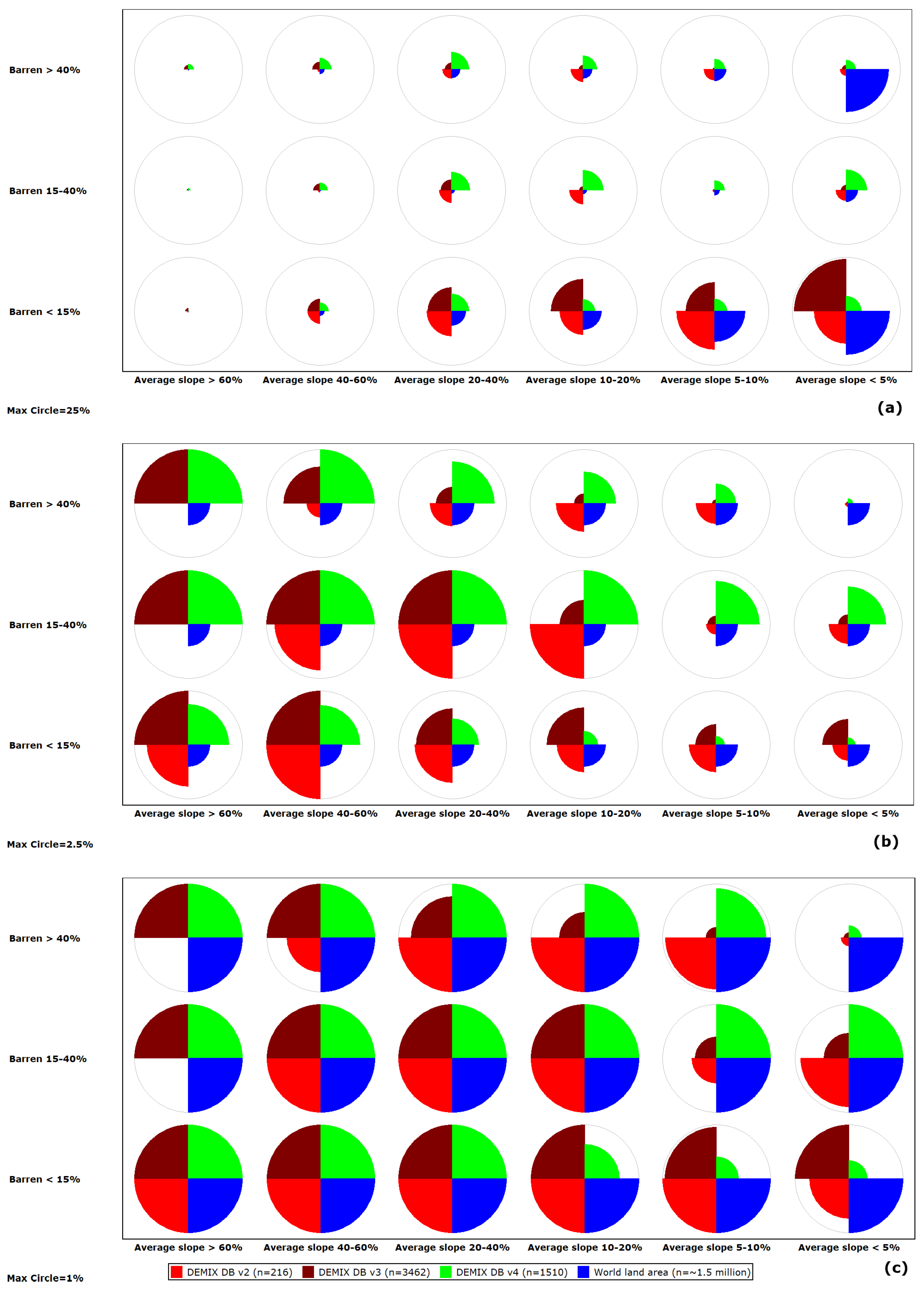
The world has about 1.5 million areas 10 × 10 km in size, and our databases contain a very small fraction of the potential test tiles, ranging from about 0.01% to 0.23% for the different versions. Many landscape characteristics determine how well a DEM represents reality, with slope and land cover among the most important. Figure 5 shows tiles broken into 18 bins, 6 for slope and 3 for the percentage of the tile that is barren. Colored sectors of the pies show the entire world, and the sample tiles in our three databases, version 2 [18,50], version 3 [25,49], and version 4 [51]. Even with this simple division into bins, we cannot show the data in a single scaling, so we show three with a different scaling for the maximum percentage of tiles in each bin. Figure 5a sets the maximum radius at 25%. Almost 50% of the tiles in the world have an average slope less than 5%. Only version 3 of our database comes close to this percentage of low-slope tiles, because of its over-emphasis on coastal tiles to evaluate DTMs created for that environment [25]. Figure 5b sets the maximum radius at 2.5% of the tiles to emphasize where the sampled tiles over-represent the world distribution, with values over 2.5% truncated. Figure 5c sets the maximum radius at 1% of the tiles to emphasize where the sampled tiles under-represent the world distribution, with values over 1% truncated. The earliest version 2 of the database severely under-represents the steepest categories, because its 126 tiles were not sufficient to include all 18 bins.
The current version of the database has between 8 and 144 tiles in each of the 18 bins. We feel that over-representing some bins to have a sufficient number of tiles to show how the test DEMs behave in different landscapes is more important than having an exact representation to match the global distribution among all 1.5 million potential tiles. Rigorous testing of this selection of categories will be the subject of further research.

2.5. Test DEMs Considered

Table 3 shows the DEMs considered. We will concentrate on four DEMs: CopDEM, ALOS, FathomDEM, and GEDTM v1.2. We limit discussion of FABDEM (included in version 4 of our database [51]), because FathomDEM proves to be much better and was produced by the same group. By limiting most of our graphs to 4 DEMs, the differences among them are much clearer. For anyone who wants, version 3.5 of our database [26] includes EDTM [52,53] and two earlier versions of GEDTM [22,23], which we will briefly discuss later.

2.6. DEMIX Database Version 4

The new version of the DEMIX database [51] contains four main tables, which use different sets of criteria, using the new tiling system based on projected coordinates.
The four tables have distinct purposes:
  • Difference distributions for elevation, slope, and surface roughness. The provides continuity with [18,25], but has limited usage in this paper because FUV provides better results [25]. For readers who want, it includes statistics like RMSE and LE90 for elevation, slope, and roughness, as well as the signed mean and median differences.
  • FUV for a mixed suite of LSPs chosen to sample the full range of LSPs calculated from DEMs. These provide better rankings of the test DEMs, an estimate of the robustness of LSPs, and suggest that some LSPs should be used with caution.
  • FUV for the partial derivatives used for slope, aspect, and curvature. These results support our recommendations about LSPs.
  • FUV for the full suite of integrated curvature measures [48]. The slopes and curvatures in this table differ from those in the mixed suite of LSPs, which use computations with a more traditional, smaller window and lower-order polynomial. It is beyond the scope of this paper to compare the different slope and curvature algorithms, but our results will address the utility of this large suite of measures.
All of the criteria names use computer-friendly versions, which can be directly used in the computer algorithms and for computer output in tables and figure labels. While a carefully formatted name like ( k n ) s s has a long tradition in science, the introduction of computers makes a variable like KNSS much easier to follow between a paper and the computer source code used.
While working to understand the multiple versions of GEDTM, we created a preliminary version of the database, which includes EDTM and several versions of GEDTM [26]. Interested users can use it to try to understand the development of GEDTM.

2.7. Criteria Used for Evaluations

We exclusively use comparisons of every pixel in the DEM with a reference grid, for both the elevations and with LSPs derived from the DEM. A huge number of LSPs have been proposed, and we use a number with different purposes and characteristics (Table 4). We use a number of open source GIS tools for computations: MICRODEM v2025.11.27 [42,47], Whitebox v2.4.0 [59], SAGA v9.3.0_x64 [60], and lsp-calculator v1.1.1 [45,46].

2.8. FUV Example

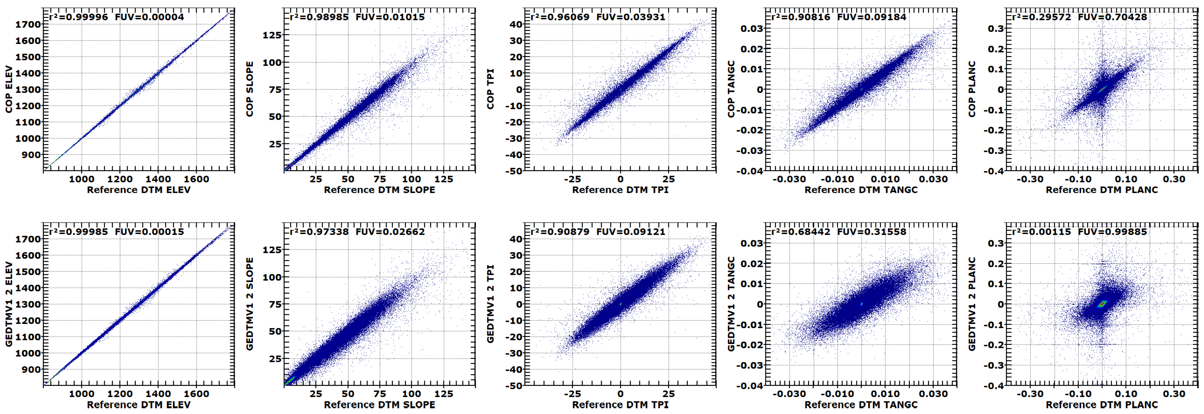
To provide an intuitive understanding of FUV introduced in [25], Figure 6 shows scatter plots for tile UTM_11N_x63y395, in the State Line area of southern Nevada. We compare each DEM with a reference DTM with the same pixel geometry; in this case, both test DEMs use SRTM geometry. In addition to the elevation grids, we compute 4 LSPs for each reference and test DEM. Using every pixel in the grids, we compute the Pearson correlation coefficient r2 and the FUV (1 − r2), both of which range between 0 and 1. This tile is 83% barren, with no urban or forested pixels, and the CopDEM DSM should be very close to a DTM. Figure 6 shows CopDEM (top row) and GEDTM (bottom row) compared to the reference DTM, with the r2 and FUV values shown in the upper left corner. For elevation, the differences do not appear until the 5th decimal place, but show the same patterns as the other criteria for the rankings of the DEM. In this case, the changes to elevation for GEDTM produce worse results than the CopDEM DSM.

3. Results

The structure of the DEMIX database version 4 allows us to investigate a number of factors:
  • Differences among test DEMs.
  • Different responses among LSPs used as criteria.
  • Characteristics of the landscape in each test tile (average slope, average roughness, percent barren, forest, urban).
The multi-dimensional nature of the database requires us to be selective in what we can show. We will briefly discuss the construction of each figure, so it is clear what is on each axis, and the different filters applied to the data within the graph. Some of the graphics are similar to those used in [25], and others are new in this work. The richness of the database requires multiple graphs, and in some cases multiple axis scalings to show the range of information.
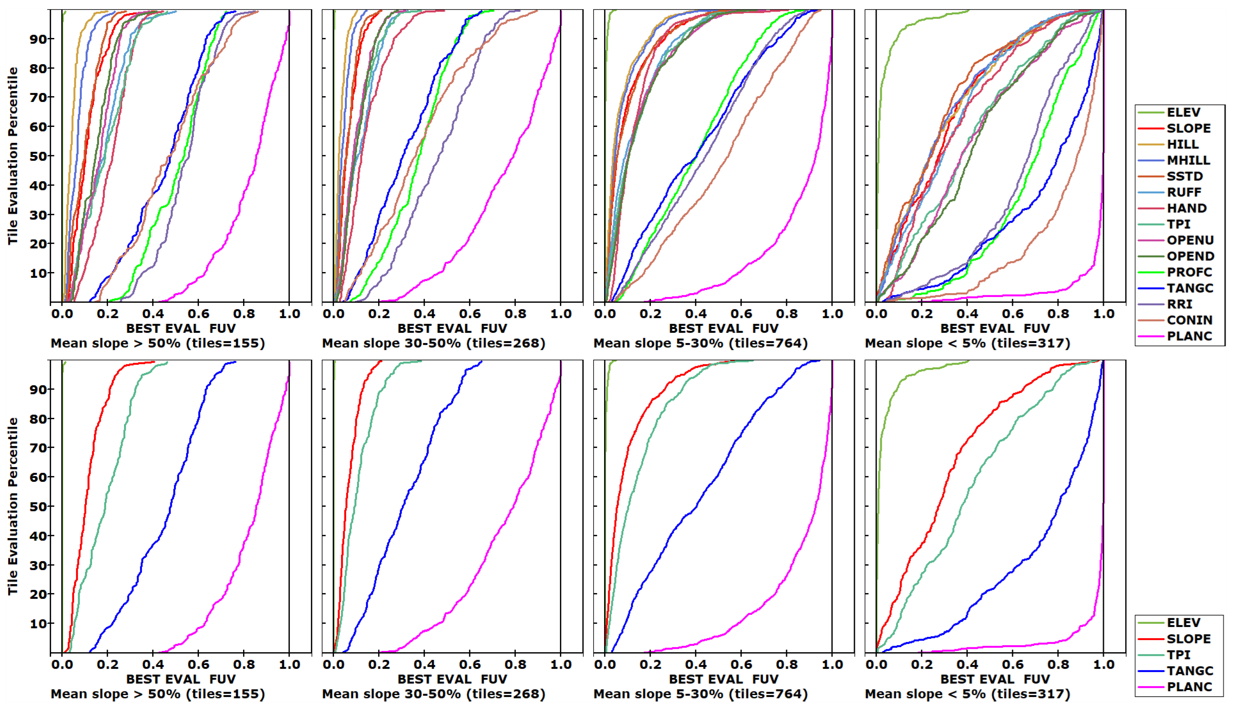
Figure 7 shows all the LSPs computed for all the test tiles, with the FUV shown on the horizontal axis and the best matches on the left side of the graph, for four slope categories. The tiles are ordered from those that best match the reference DTM at the bottom of the vertical axis, and those with the worst matches on the top. The figure shows only the best evaluation among all the test DEMs, to concentrate on the responses of the LSPs without initially considering the differences among the test DEMs. The LSPs fall into four groups across all of the slope categories considered. In the lower panel of Figure 7, we selected five LSPs that exemplify the range of LSP behavior. Except for low-slope tiles, ELEV has FUV values close to 0, which require axis rescaling to show the differences among test areas or the different DEMs. SLOPE, TPI, and TANGC show progressively lower FUV values, and PLANC has significantly lower FUV values. For many of the figures to follow, we feature results from four LSPs, which show the range of matching the reference DTM from best (ELEV), through two intermediate (SLOPE and TANGC), to the worst (PLANC).

3.1. Best Evaluation in Each Tile

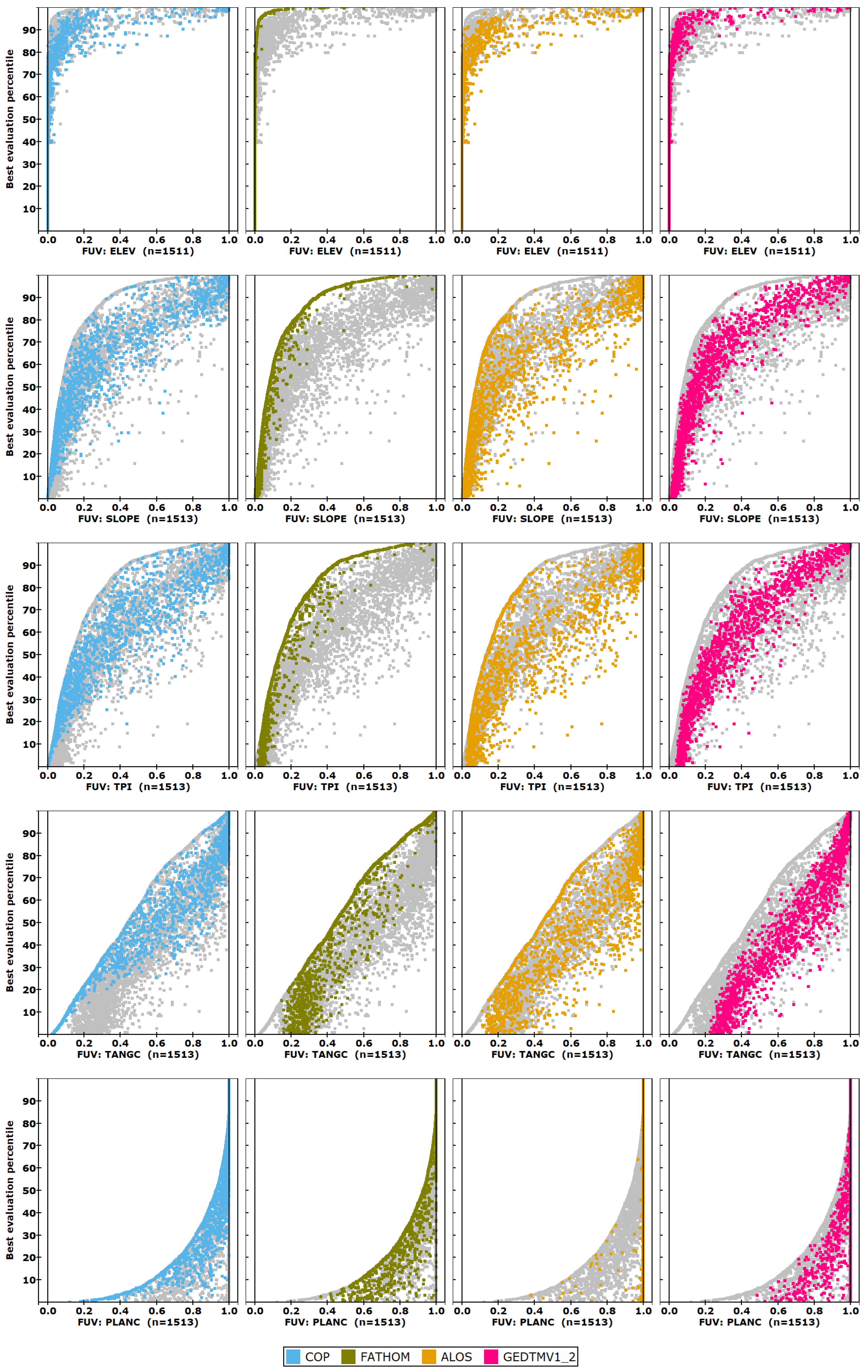
The graphs in Figure 8 show the four test DEMs in the columns, and five comparison criteria in each row to show representative patterns. Each graph has about 20,000 evaluations, so it provides only a general pattern that is still informative. The graphs demonstrate how well each criterion matches the reference DTM, and which DEM performs best. Because of the large number of data points, all the DEMs would overlap and cannot be shown on a single graph. The gray points show all the data, with each DEM in a different color in one column of panels.
The best results have an FUV close to zero, and the tiles are sorted by the best FUV from any of the DEMs, and the y-axis is organized by the percentile of the best tile, with each test DEM plotted on the same horizontal line. A DEM that always most closely matched the reference DTM would be on the left edge of the cloud of data points, and those that did not match well would be spread across the cloud.
On top of all the graphs, a percentage of the tiles shows poor agreement for all of the test DEMs with the reference DTM. For elevation, most tiles show FUV close to 0, while for plan curvature, very few tiles show FUV close to 0, and the majority have FUV close to 1. This indicates that elevation is represented more accurately by the test DEMs overall than plan curvature, and plan curvature should be used with caution. The best DEM will be on the left side of the graph, which has the best FUV, in a narrow band; for SLOPE, this would be FATHOM DEM. GEDTM performs poorly on both curvature LSPs.

3.2. Evaluations Sorted by Tile Average Characteristics

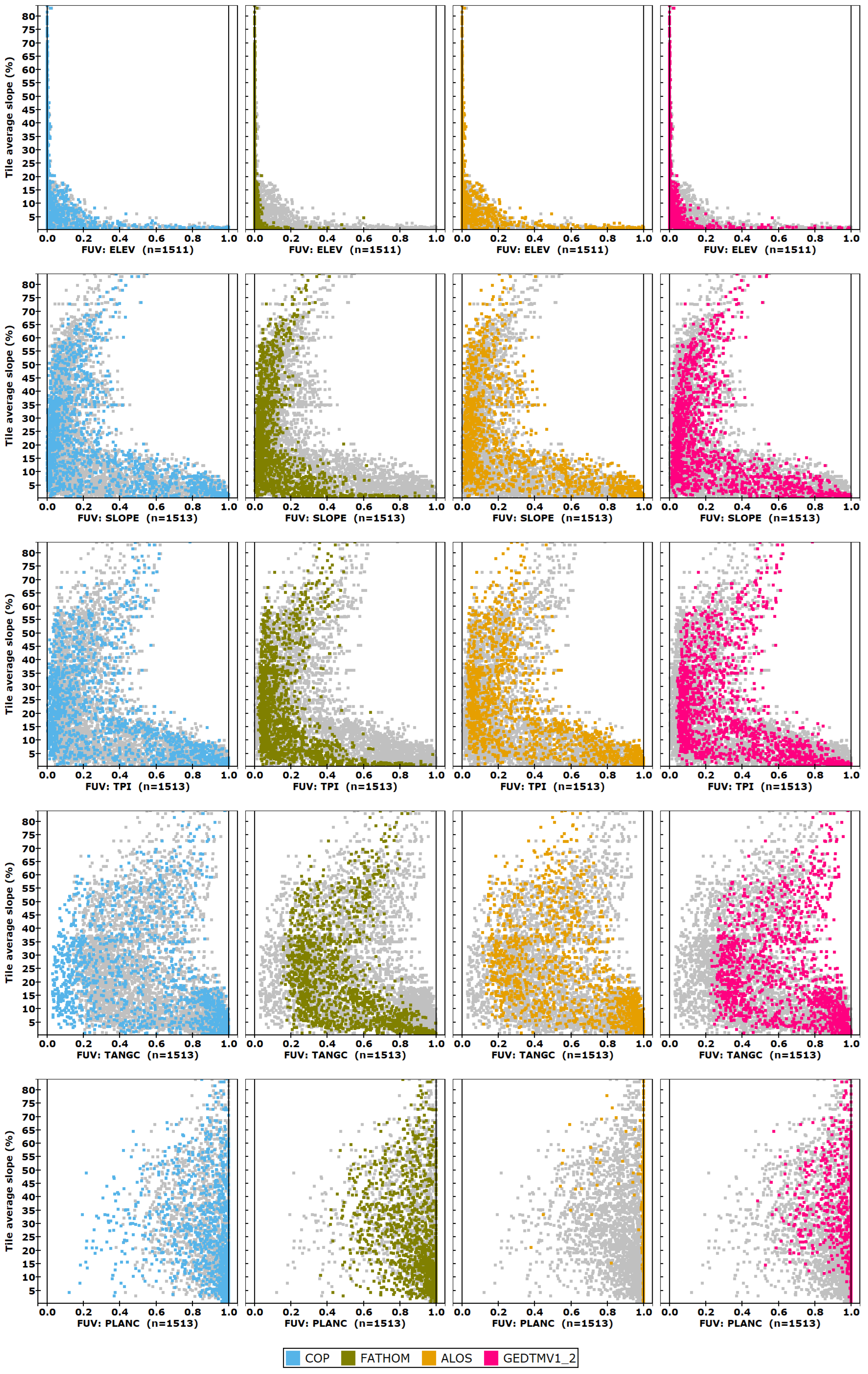
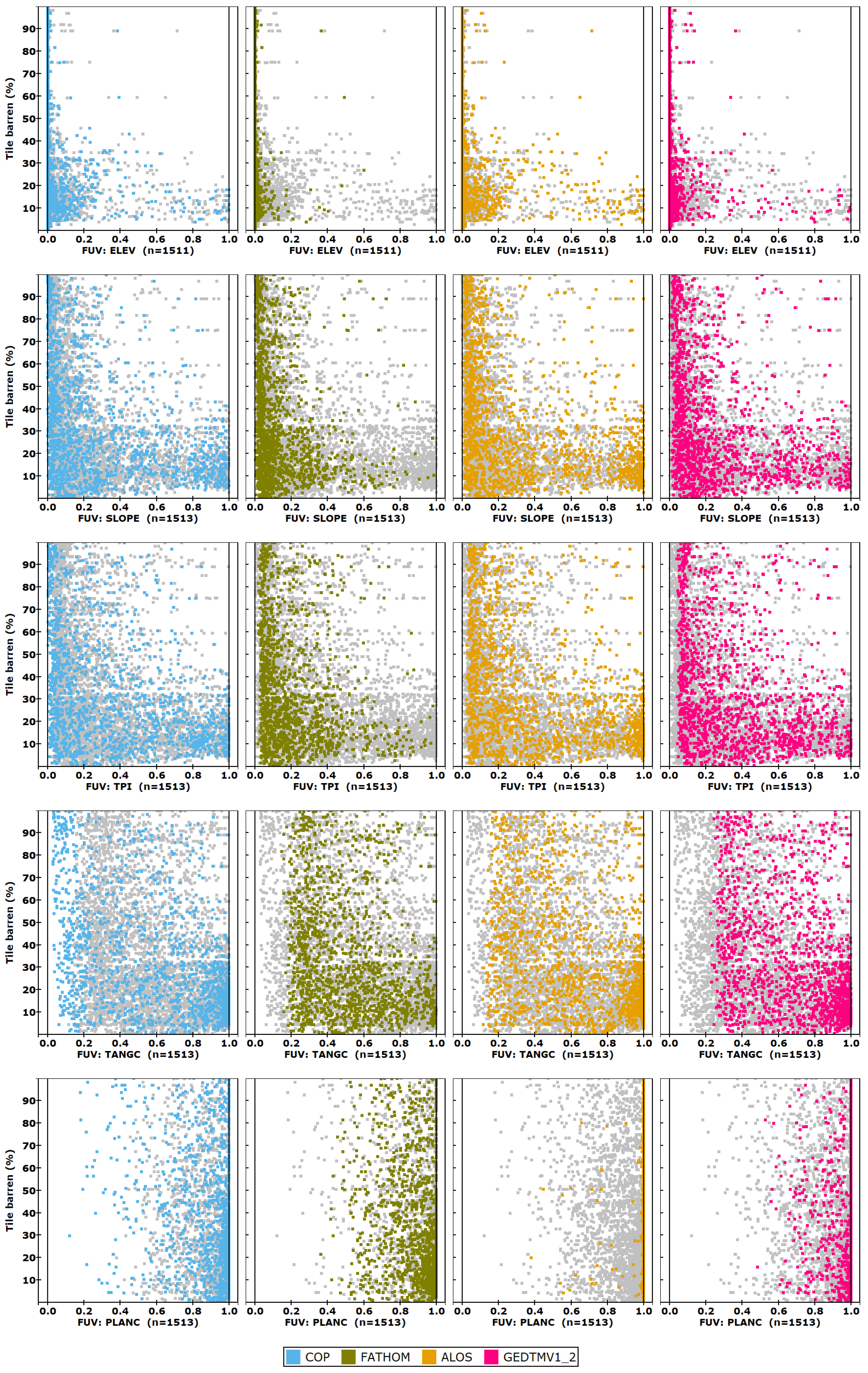
Tiles can be sorted by average characteristics to see where the test DEMs perform better, in Figure 9 for average slope and in Figure 10 by the percentage of the tile with barren landcover. For average tile slope above 20%, for ELEV, all the test DEMs have very small FUVs, while at the smallest slopes, all the test DEMs show a large range of FUV from 0 to 1. For PLANC, none of the test DEMs have very small FUV, with the AW3D30 DEM essentially uncorrelated with the reference DTM. For tile barren percentage tile above about 40%, for ELEV all the test DEMs have very small FUVs.
The deterioration of SLOPE, TANGC, and PLANC for steeper slopes in Figure 9 is clear from the “c” patterns in the curves with the inflection point at about 30–40% average tile slope.

3.3. Evaluations Lumped by Terrain Categories

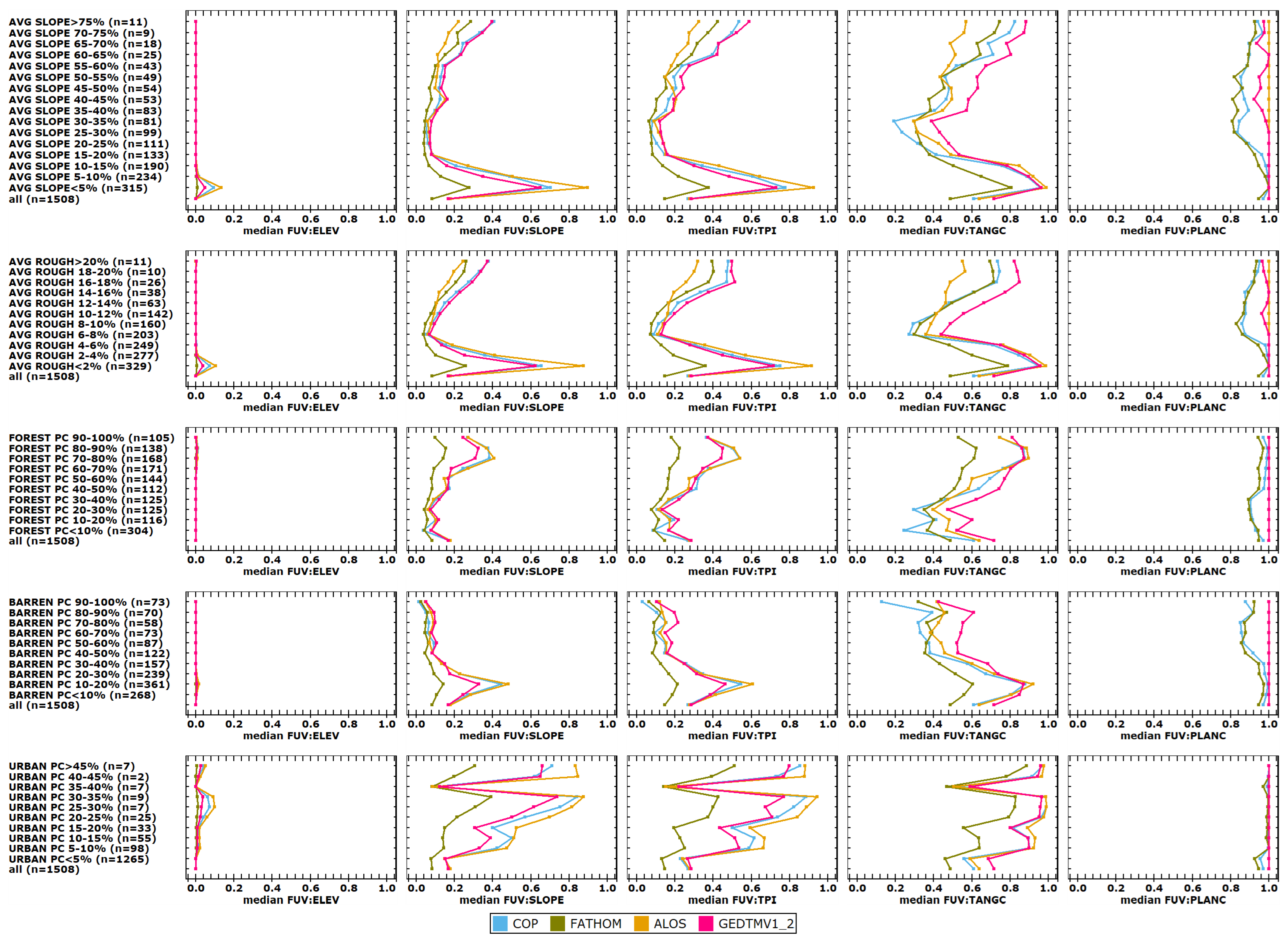
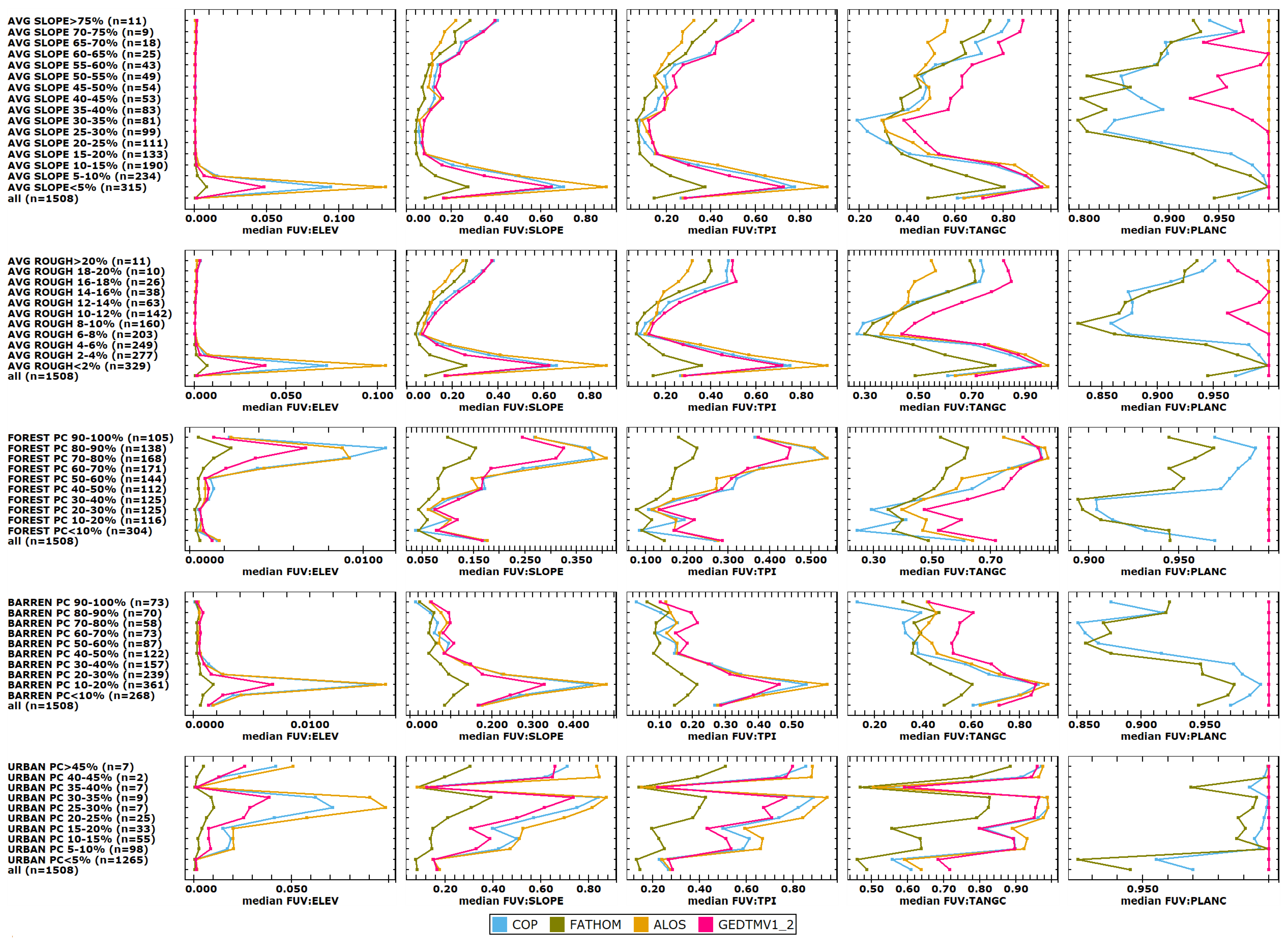
Graphs in the previous section have over 1500 tiles for each test DEM, and demonstrate broad trends. Aggregating tiles into bins better reveals trends, with the average FUV for all tiles that match the terrain filter. Figure 11 and Figure 12 show the five representative LSP criteria with a number of divisions for each of the five terrain categories. The legends on the left include the number of tiles in each plot, and the graph plots the median for all tiles.
Figure 11 shows that for elevation, all the averages for rough tiles and those that are not gently sloping have very similar small FUV values. Some workers have interpreted this as meaning that FUV does not work for elevation, but this is too simplistic an interpretation. While this figure does not differentiate the performance of the DEMs in terms of elevation, it clearly shows the progression in performance of the four LSPs. Figure 12 restricts the range on the horizontal axis to emphasize the differences among test DEMs at the expense of not showing the difference in LSP performance. Even at this scale, for elevation, however, the poor performance of low average slope and low average roughness tiles masks differences in the steeper, rougher tiles. For elevation, the poor performance of the two test DSMs (ALOS and CopDEM) shows up in tiles with low slope, low roughness, limited barren pixels, and high forest and urban land cover.

3.4. Performance Ranking of LSP Criteria

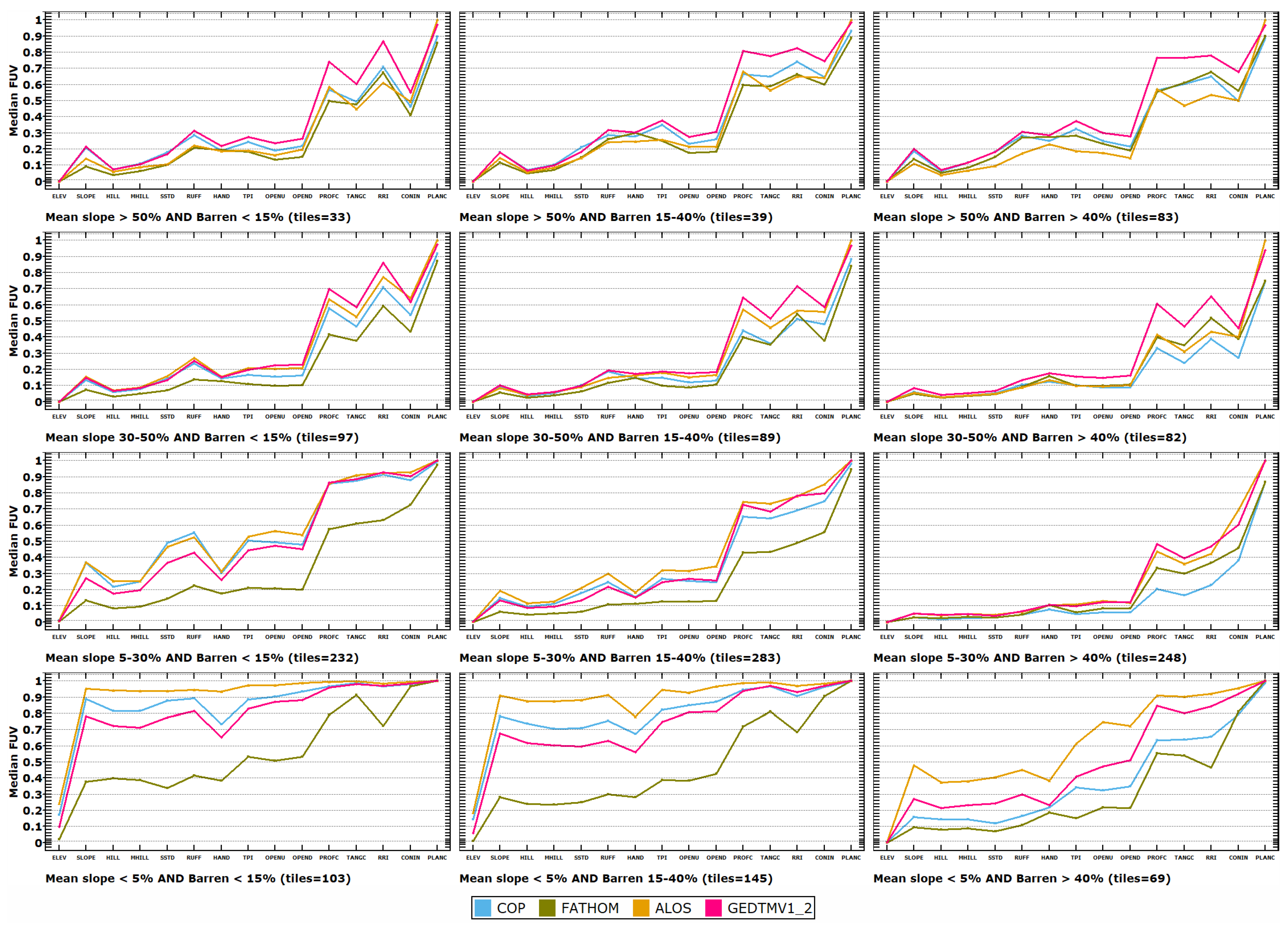
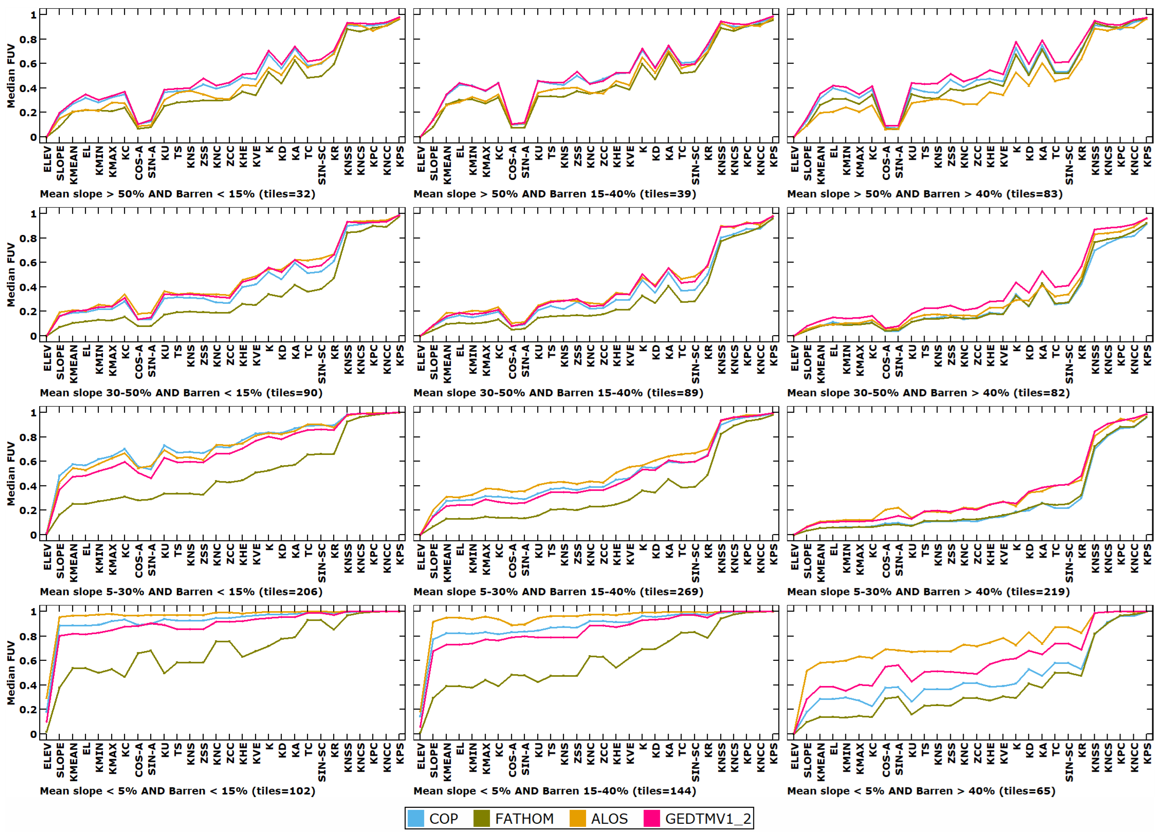
The LSPs used as criteria can be ordered based on the average FUV, from those that closely match the reference DTM to those that barely match it. While the FUV values vary among test DEMs and with tile characteristics, the general trend of the ordering is consistent for all the individual graphs in Figure 13. The graphs have median FUV on the vertical axis, from 0 (best) to 1 (worst), and the LSP criteria on the horizontal axis. The graphs are arranged with mean tile slopes in the columns, and the percentage barren in the rows. Colors show the test DEMs. The label below each graph shows the filter with the slope and barren percentage, and the number of test tiles that match the filter. Lines connect the points on the graphs to clearly show the increasing FUV values in the criteria from left to right, and better show the results compared to merely plotting the data points.
The ordering of the criteria goes from those that most closely match the reference DTM to those that barely match. The graphs show some small reversals instead of a steady increase, because the results vary somewhat by test DEM and applied filters. The criteria generally follow the order in which they appear in Table 4, Table 5 and Table 6, with the best at the top of the table, and in the figures, the best will be on the left.
Comments on particular LSPs:
  • The best criteria depend only on simple operations with first partial derivatives, SLOPE, and the two hillshades, which depend on the normal vector to the earth’s surface, a 3D representation of slope and aspect.
  • A number of studies list profile (KNS) and tangential (KNC) curvature as basic LSPs [63,64]. These are among the best-performing curvatures (and very close to the best curvature LSPs in the entire suite of curvatures to be discussed later).
  • In general, the curvature criteria, requiring second-order partial derivatives, perform more poorly compared to the other LSPs in Table 4.
  • ALOS generally performs worse than CopDEM, and its integer resolution elevations provide coarser resolution, making it harder to match the reference DTM.
  • Roughness is a complex metric without a common definition, and two of our metrics have been used for roughness, RUFF (standard deviation of slope) and RRI. RRI is more sensitive, with a larger FUV.

3.5. Effect of Terrain on Criteria Performance

Figure 13 shows the FUV on the vertical axis and the criteria on the horizontal axis. The figure shows four average tile slope categories in the rows, and three categories for average tile barrenness in the columns. Colors show the test DEMs.
FUV increases with the criteria from right to left in each graph; the best results are generally with moderate slopes and high barrenness. Fathom DEM is almost always the best performing, with GEDTM generally having the highest FUV and hence worst at matching the reference DTM.

3.6. Effect of Terrain on Partial Derivatives

Many LSPs (slope, aspect, curvatures) require partial derivatives computed from the DEM, and other complex LSPs incorporate these derivatives. Nine first through third order partial derivatives can be computed [46] for a 5 × 5 window, and the only required parameter is the choice between a third or fourth order polynomial. Traditional computations have generally used a 3 × 3 window and a second-order polynomial; it is beyond the scope of this paper to compare the two approaches. Using the same method for all the DEMs and the entire suite of partial derivatives and subsequent LSPs allows us to investigate the role of both different DEMs and landscape parameters without necessarily endorsing the replacement of the traditional algorithms we used in the first mixed database table.
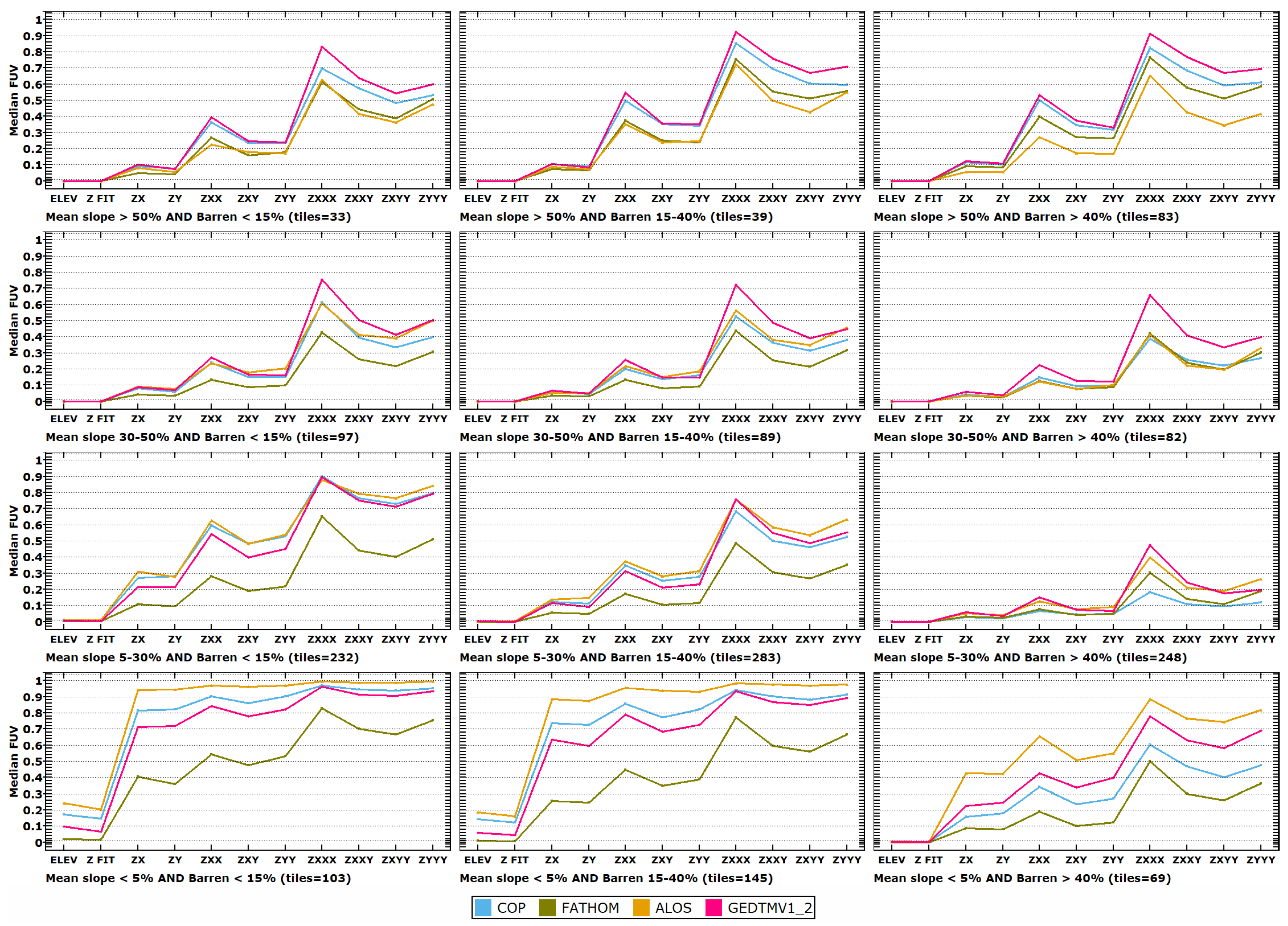
Figure 14 shows the computed partial derivatives, plus elevation and the fitted elevation computed from the least squares quadratic surface, on the horizontal axis. The partial derivative names given in Table 5 are computer-friendly without any subscripts, Greek letters, or parentheses [46]. The vertical axis has FUV. The figure shows four average tile slope categories in the rows, and three categories for average tile barrenness in the columns. Colors show the test DEMs.
Low slopes (bottom row) have the highest FUV, meaning the test DEMs are not very similar to the reference DTM. Low barrenness (left column) has a similar effect. Among the partial derivatives, the FUV values increase from the first to the third-order partials. The fitted z value has similar values to the elevation, and is close to 0 except for the gentlest slope category (bottom row).
FathomDEM performs best across all the panels. While GEDTM is best in the panels in the lower left corner, in the others it is generally the worst, suggesting it only works well in low slopes and low barren tiles.
The FUV in all the graphs increases from left to right, with the increase in the order of the partial derivatives. In Figure 14, the FUV for partials ZXX is consistently larger than ZYY, and ZXXX is even more noticeably larger than ZYYY. Interestingly, this is not the case for ZX and ZY. We suspect this may be due to the smaller spacing in these DEMs in the x (east-west) direction, and how the sensor footprint, the DEM processing, and the posting to a rectangular grid cause an increase in anisotropy with the higher-order partial derivatives.

3.7. Effect of Terrain on Curvature Measures

Recent work has established a framework for curvature computations, bringing order to what had been a number of incompatible definitions and software implementations [48]. Further work related curvature measures to energy relevant to land surface segmentation [65], and created software [45,46] to compute the entire suite of 28 curvatures and related measures listed in Table 6. As with the partial derivatives in the previous section, we use computer-friendly criteria names instead of those in [46]. Because of challenges with circular statistics, we did not use aspect, but have the sine and cosine of aspect, which do not suffer from those problems.
Our methodology allows us to evaluate the entire suite of curvature LSPs and see how they compare with global DEMs and a reference DTM. The slopes and curvatures used in this analysis differ from those computed in the mixed suite, where we used more traditional slope and curvature measures computed with a smaller window and a lower-order polynomial. We are not advocating here for which computation algorithm is more appropriate, but want to investigate how the use of increasingly high-order polynomials affects the confidence in the LSP results.
Figure 15 shows the results, similar to those for the partial derivatives (Figure 14). Like the partial derivatives, the curvatures have increasingly higher FUV with higher orders of partial derivatives used in the computations. Two of the curvatures computed with second-order partials have FUV values that match or even exceed those computed with third-order partials, which all have FUV close to 1. KPC and KPS are both divided by the sine of the slope, which will cause large changes in the computed value with small changes in elevation between the test and reference DEMs, and lead to the test and reference LSPs being almost uncorrelated and producing an FUV near 1.
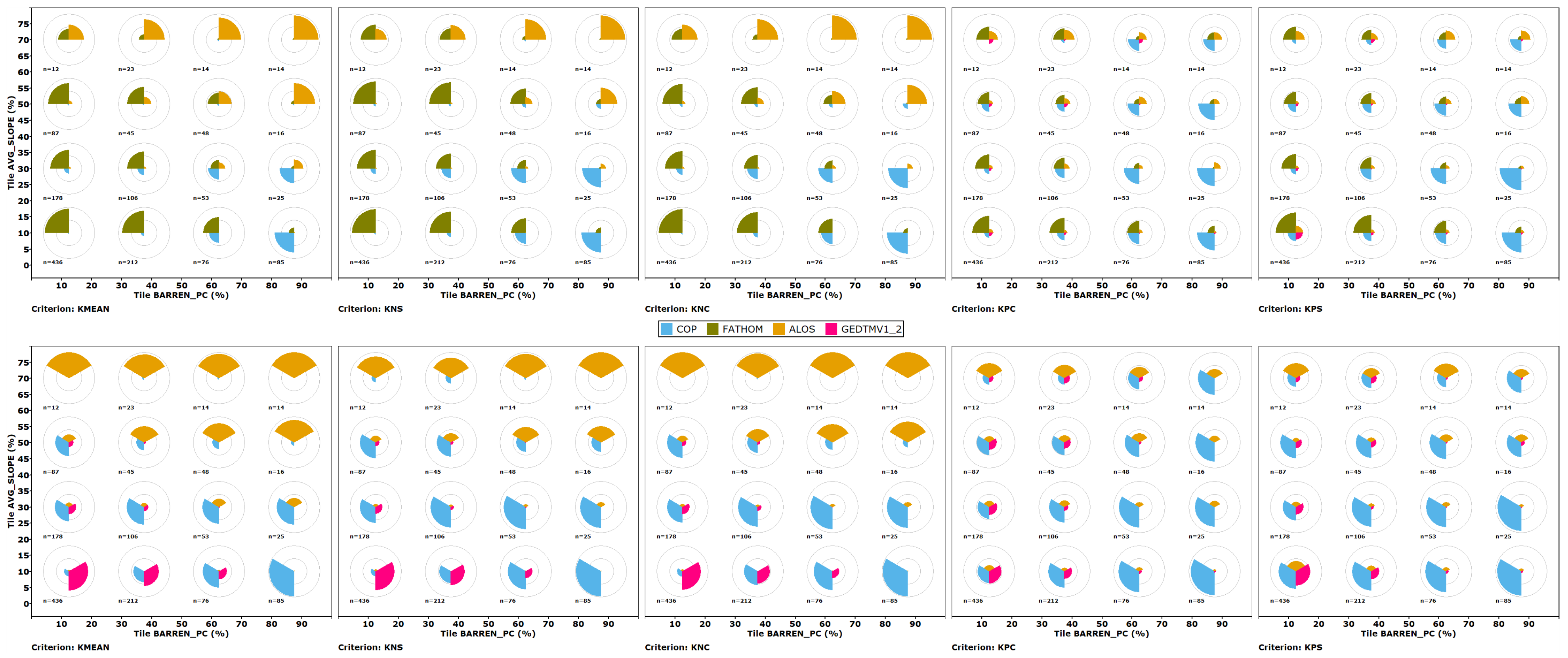
FathomDTM performs consistently the best. For low slopes and moderate barrenness (lower left panels), GEDTM is the second best, but it is the worst for high slopes and moderate to high barrenness (the five upper right panels), with the same performance as with the partial derivatives used to compute curvature. ALOS is consistently good for very high slopes.

3.8. Comparing Curvature Algorithms on FUV

Our use of two distinct algorithm families for slope and curvature allows comparison of the algorithms and their sensitivities. The mixed suite of LSP criteria included slope and three curvature measures computed with the traditional Evans algorithm (3 × 3 window and 2nd order polynomial, implemented in MICRODEM and Whitebox) and the LSPcalc algorithm (5 × 5 window, 3rd order polynomial [46]). Figure 16 shows how the results compare for tiles in four slope categories. For the traditional method, we use the descriptive names and note their correspondence with the newer proposed names. The graphs show the DEM with the best evaluation in each tile, which in most cases will be FathomDEM.
The results show the complex interplay of terrain characteristics and LSP algorithms. We consider the better algorithm as the one with the lowest FUV, where the test and reference DEMs produce the most similar results.
  • For the tiles with the shallowest slopes, the LSPcalc algorithm performs best for all four of these criteria. These tiles perform poorly for all the criteria, because the algorithms amplify the small elevation differences between the test and reference DEMs. The combined effect of a larger window and higher-order polynomials lessens the differences between the test and reference DEMs.
  • For the higher slope tiles, the Evans method generally works slightly better for SLOPE and PLANC/KPC, and worse for PROFC/KNS and TANGC/KNC.
  • PLANC/KPC performs poorly for both algorithms, and should be used with caution.

3.9. Limitations of Simple Difference (Error) Metrics

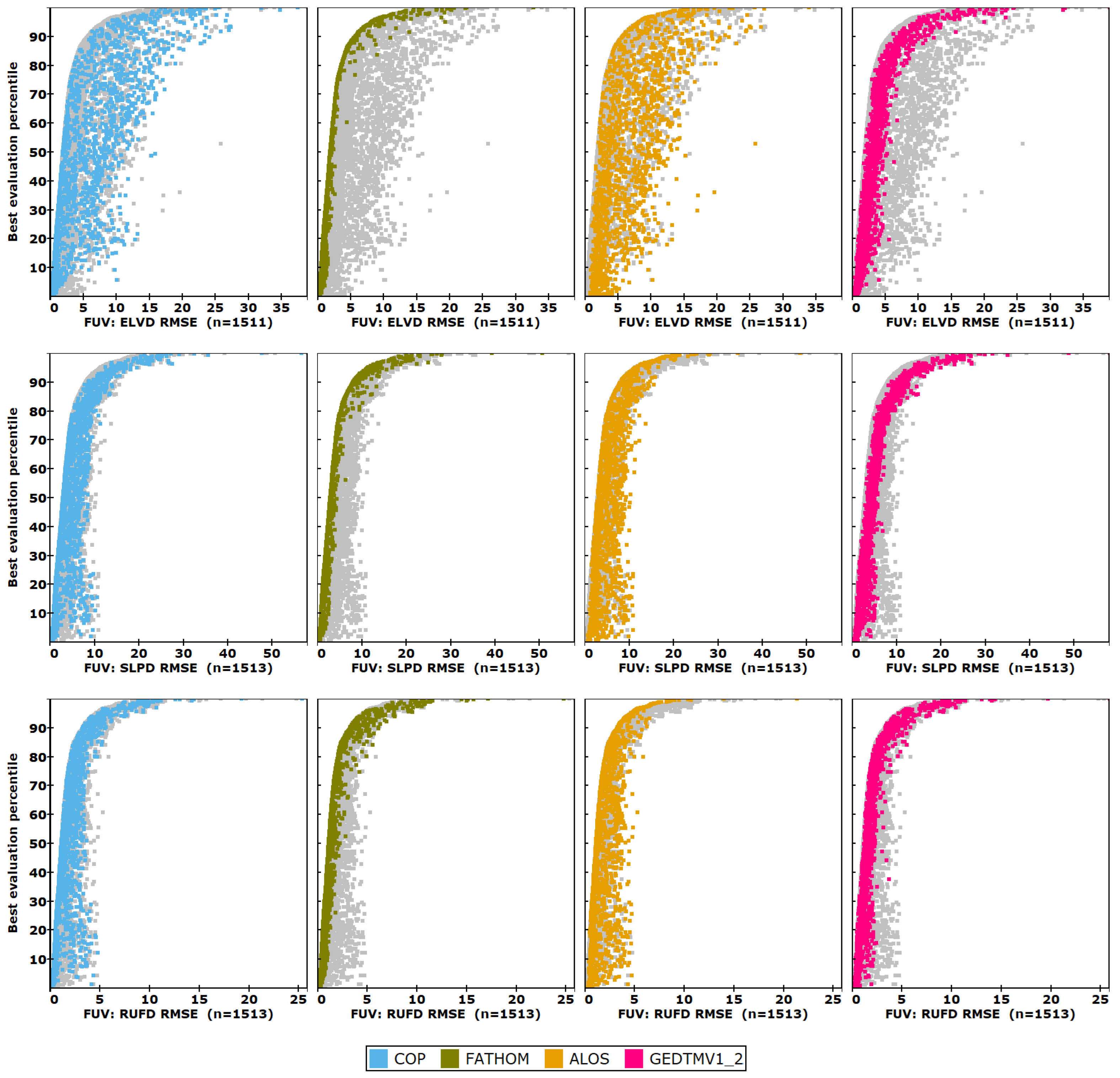
Most comparisons of the global DEMs focus on a few metrics of the difference between the test DEM and reference data, generally using just the elevation data. GEDTM used only RMSE of elevation [5] while FathomDEM used mean error (ME), mean absolute error (MAE), and root mean squared error (RMSE) of the elevation, slope, and roughness grids [19], the same LSPs used starting with the first DEMIX results [18].
Figure 17 shows the RMSE for elevation, slope, and roughness for all the test tiles. FathomDEM clearly best matches the reference DTM. This figure does not show how the results reflect the characteristics of the test areas, which influence the results. MAE, RMSE, and LE90 provide very similar results.

4. Discussion

The database with our results demonstrates several things (1) which DEMs more closely match the reference DTM, (2) how terrain characteristics affect different DEMs, and (3) the degree to which LSPs match the reference DTM, and which LSPs suffer most from noise in the DEMs or extreme sensitivity in the algorithm and should be interpreted with caution.
DEM creation has different challenges depending on slope and land cover, and the importance of those has been debated [66]. We think the average slope for the tile is the best overall indicator, and we show that it is the largest number in our graphics. To some extent, surface roughness is complementary to slope, even if the two are many times correlated, and we need to simplify the graphics we present. The second most important characteristic would be the percentage of the tile that is barren, and we show that along with slope in many two-dimensional grids of individual graphics. Rather than simply showing the best DEM, we show the comparative results for each DEM. The percent forested would generally be the inverse of percent barren, but the correlation is not perfect because additional landcover categories do not map easily to a simple binary classification. Other land cover categories are generally much less important, and the urban areas present particular problems for spaceborne sensors. Overall, we suspect that landcovers other than barren and forest are most likely to occur in low slope areas, which have the highest FUV values.

4.1. DEM Winners—Choosing the Best DEM

Each record of the DEMIX FUV database contains a tile name, the criterion, and numerical evaluations for each test DEM. Evaluations range from 0 (perfect match with the LSP computed from the reference DTM) to 1 (random correlation with the reference LSP). Because the evaluations are floating-point numbers, we assign a tolerance (Table 4) for results that we consider ties.
Previous work has shown that FABDEM was generally the best DEM, with CopDEM a close second [18,66]. The new FathomDEM was created by the same group as FABDEM, and our results show it is clearly much superior and shares the same restrictive license. To clearly show our results, most of our graphics will show only four DEMs: FathomDEM, CopDEM, ALOS AW3D30, and GEDTM, but the database includes FABDEM [51].
Analyzing the results in the databases requires a number of subjective decisions:
  • Which LSPs to use, either the ones we computed or others.
  • Which of our four tables to use.
  • The tolerance to decide if evaluations are different or tied. The tolerances represent our subjective estimate and are defined in the parameter tables, and the evaluation software is set up to allow easy changes to the tolerances without recompiling the code or recomputing the database.
  • Whether to average multiple criteria for a single evaluation, or keep each criterion separate.
  • The landscape categories to consider.
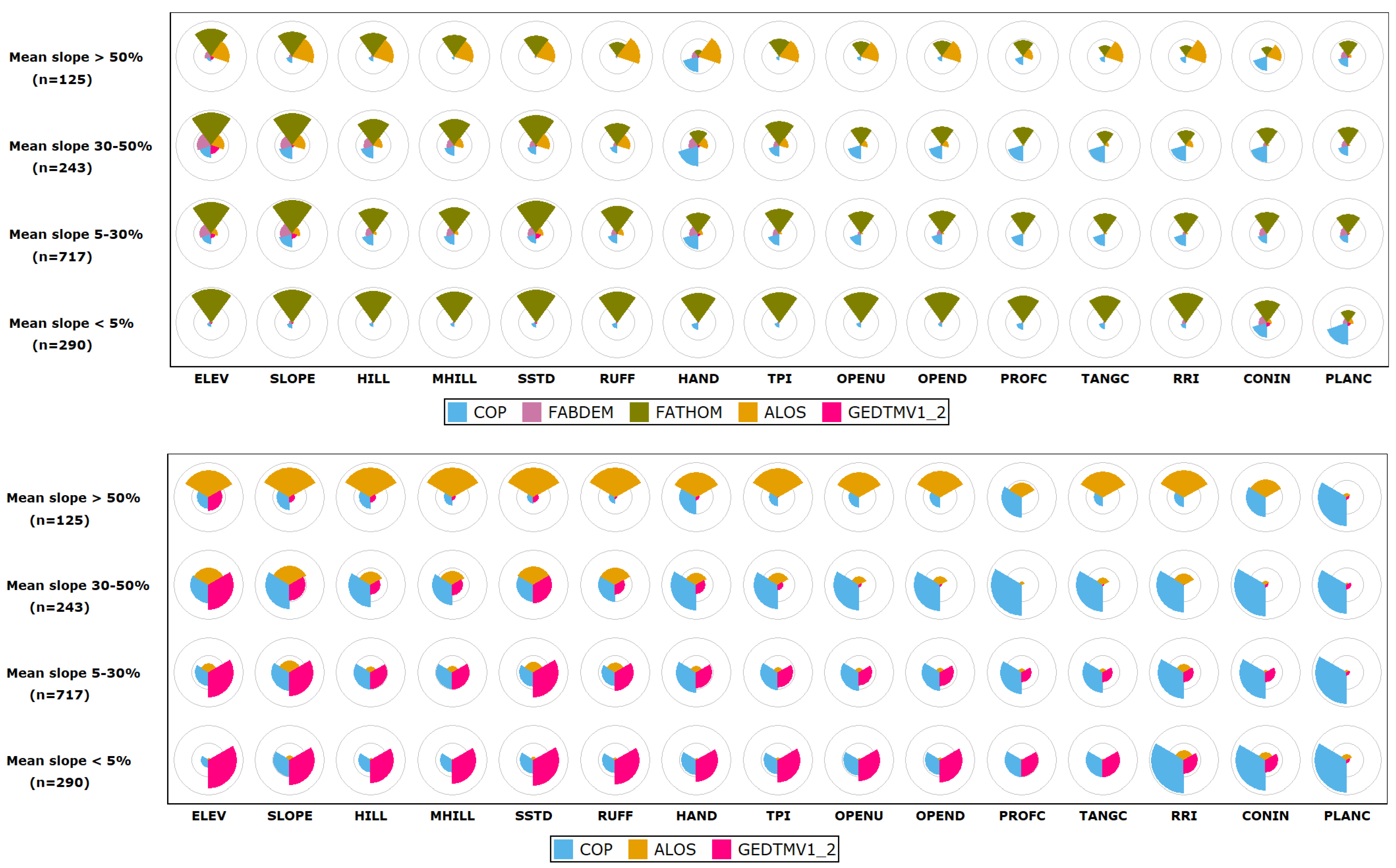
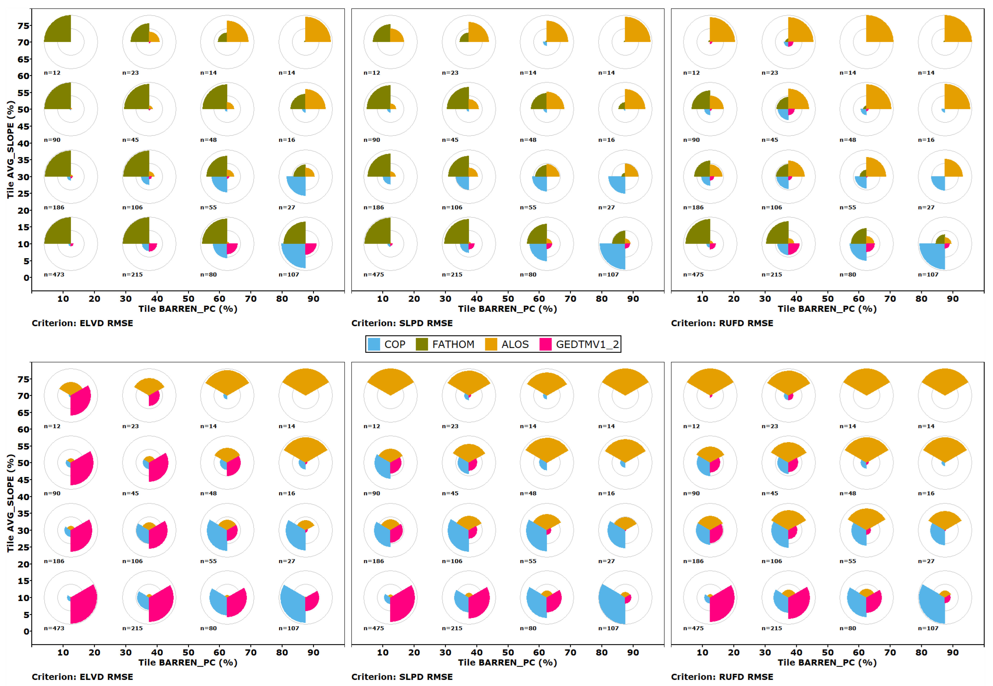
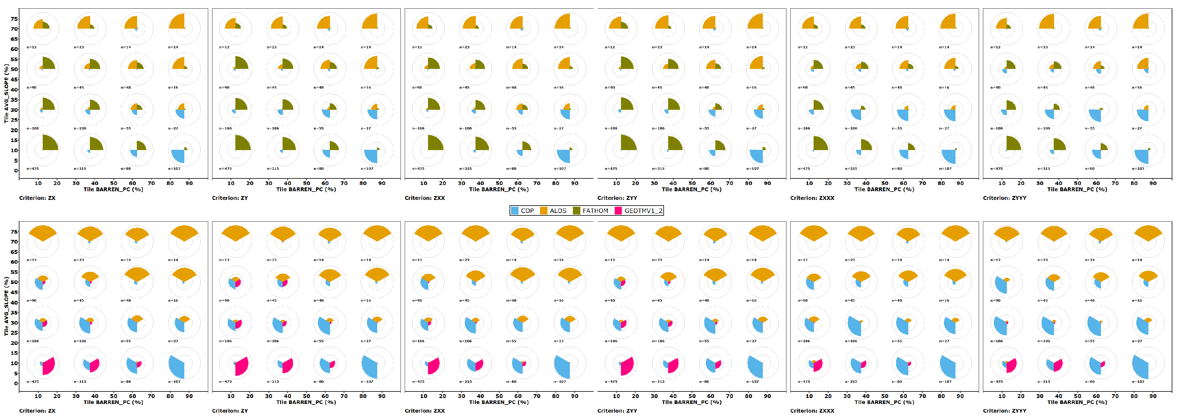
We present the results of our DEM ranking with a series of pie charts. Slices in each pie represent the DEMs, with the size of the pie showing the percentage of tiles where the DEM performs best or we consider it to be tied based on the applied tolerances. Gray circles at 50% and 100% help gauge the results, which for all the DEMs can sum to more than 100% because of ties. Each comparison has two panels: a top one with all 4 DEMs, and a lower one with the three DEMs with unrestricted licenses. Each panel has four slope categories, because the DEMs perform differently depending on the slope, and we find slope to be the most important terrain characteristic (Figure 14, Figure 15, Figure 18 and Figure 19).
When removing from consideration the restricted DEMs, especially FathomDEM, which is usually the top choice, the DEM with the second most wins does not necessarily always move into first place. The changes in rankings depend only on tiles and criteria where FathomDEM was the sole winner, and then which DEMs move into first from second place.

4.2. DEM Winners—Mixed LSPs

Figure 18 shows the winning percentage for each criterion and DEM. For users who can live with its restrictive license, FathomDEM clearly is the best choice. In the steepest category, ALOS might be a better choice, and for some of the curvatures, CopDEM might approach the results. The choice among the unrestricted licenses is less clear. For the steepest test areas, ALOS is the best, except for PLANC and CONIN, where CopDEM is best. For gentle slope areas, GEDTM is best for the LSPs on the left side of the diagram, which are mostly non-curvature measures.

4.3. DEM Winners—Difference Distributions

DEMIX has consistently argued that DEM comparisons should consider the derived LSPs that provide many of the most important DEM applications [18,25]. All versions of the DEMIX database have included statistical measures for the difference distribution for the elevation, slope, and roughness grids for each test area [18]. In Figure 19, we show pie diagrams with the best DEM considering RMSE for each of the three LSPs.
Most comparisons of DEMs use statistics for the elevation differences with reference elevations, often with a small number of points, or a grid comparison with other global DEMs. FathomDEM considered MAE, RMSE, and LE90 to evaluate against four other DEMs [19]. GEDTM used mean error and RMSE compared to GNSS station records [5]; because of the small number of control points, the values cannot be readily compared with other work since the control points might not be randomly located, particularly in steep areas where differences among the DEMs tend to be largest.
Figure 19 shows the RMSE for the three criteria used.
  • FathomDEM is generally the best, considering all four DEMs. CopDEM is best in many tiles with low slope and high barenness, and ALOS is best in high slope and barren tiles.
  • Among the unrestricted license, GEDTM performs best for low slope tiles that are not barren, ALOS best for high slopes, and CopDEM for intermediate cases.
  • The cases where ALOS is best are characterized by small numbers of test tiles. The superior performance of ALOS in steep terrain is consistent in all our results and with previous results [25,67], but such steep terrain is relatively rare globally, and the preferential use of ALOS should be restricted to those areas.
  • The three metrics considered for the difference distributions are the best, fourth, and sixth best of the criteria used in our FUV comparisons (Table 4 and Figure 7). Using more criteria, particularly for the LSPs that consistently compare worse to the reference DTM, can change conclusions from this simpler analysis using just these three criteria.
Two likely reasons for the much better performance of FathomDEM compared to GEDTM lie in the use of lidar data for training and the use of multiple criteria to evaluate their results, which could influence the tuning of the model used to generate the model. Edited DTMs that only use comparison of elevations to reference DTMs are likely to perform worse than those that look at multiple LSP criteria. In addition, the poor performance of both FathomDEM and GEDTM in the under 50% barren tiles suggests that they overcorrect when attempting to remove vegetation, to the point where the DSMs perform better compared to the reference DTM.

4.4. DEM Winners—Partial Derivatives FUV

Figure 20 shows the best DEM considering six of the partial derivative grids, excluding the two elevation criteria and the mixed partial derivatives. The FUVs for these criteria increase from left (first order) to right (third order).
If the license is no consideration, the pattern is very similar to that using the different distributions. FathomDEM is best in the lower left (low slope, not barren), CopDEM in the lower right (low slope, high barrenness), and ALOS along the top (steep slopes).
Among the DEMs with unrestricted licenses, GEDTM is rarely best, and only for low slopes.

4.5. DEM Winners—Curvatures Family of LSPs

Figure 21 shows the best DEM considering the partial derivative grids. The five curvatures were selected to show the range of agreement between those computed with the test DEMs and the reference DTM, with the best (lowest FUV) on the left and increasing FUV to the right.
For both unrestricted and restricted licenses, the patterns are broadly similar to those for different distributions and the partial derivatives. GEDTM appears as the best in very few comparisons.

4.6. Can a DSM Be “Better” than a DTM?

A DSM and a DTM should be different [1], and each has appropriate applications. A DTM is often more useful, and some national mapping agencies, such as USGS, only produce DTMs. However, just because a DTM purports to remove vegetation and buildings does not mean that it succeeded and did not make changes that moved the initial DSM farther from the lidar-derived DTM. The edited DTMs frequently only use elevation data for validation, and those elevations are typically isolated points or laser altimeter tracks. The space-based laser altimeters have much larger footprints compared to aircraft-mounted instruments, and while they can provide reasonable profiles along the track, they cannot measure across track and thus cannot accurately measure the neighborhood elevations, which are critical for most LSPs. The current generation of space-based profiling lidars differs from the more typical scanning lidar available from airborne datasets.

4.7. EDTM, GEDTM, and Precomputed LSPs

EDTM [52,53] was published as having an unrestricted license, but because it used FABDEM [58], it actually inherited a restrictive license. It is unclear if the version with the restrictive license was publicly available. EDTM did not have a peer-reviewed publication; we include it because of its strong performance in some comparisons and because it is still available. GEDTM currently has posted at least five versions, three of which are still available [22,23,24]. The documentation of GEDTM is not clear about what differs among the multiple versions, some of which are no longer available for unspecified reasons. Our final conclusion, for reasons we will develop, is that the version of GEDTM v1.2 currently available in November 2025 should not be used. Figure 1 shows the pixel locations of the 0.9 arc-second versions of GEDTM, which we recommend avoiding.
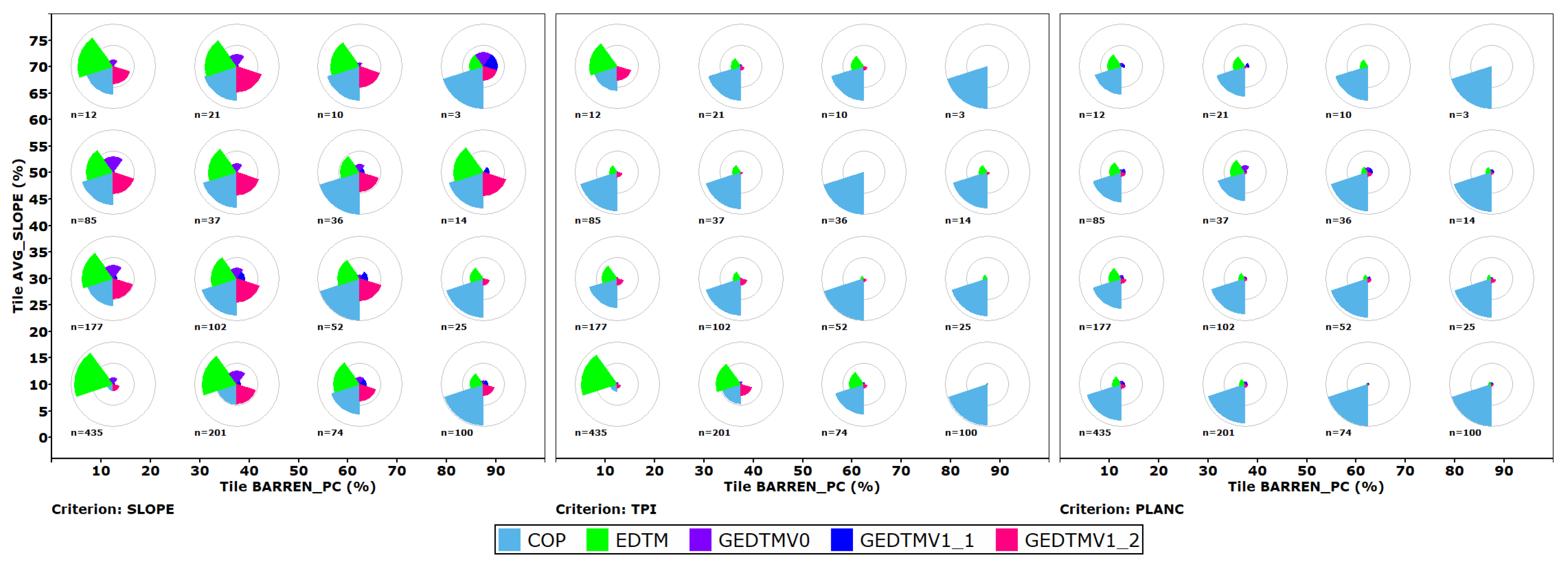
The process of creating a one-arc-second DTM frequently resembles a black box, with little clear explanation of how the algorithm works. GEDTM provides an interesting example to see how the process evolved with successive releases, even if the differences and the specifics of the early versions have not been documented. Version 3.5 of our database [26] computes statistics for three versions of GEDTM (version 0 [22], version 1.1 [23], and version 1.2 with elevations specified as meters instead of decimeters [24], as well as its predecessor EDTM [52]). Versions 0 and 1.1 of GEDTM used 0.9 arc-second spacing (approximately 30 yards or 90 feet instead of 30 m), and our comparisons used special reference DTMs at that resolution.
Figure 22 compares the EDTM and three versions of GEDTM, with CopDEM as a reference. EDTM wins in some cases, especially for the slope criterion with low barrenness, but generally CopDEM wins. The versions of GEDTM rarely win, and their comparative performance is not consistent.
EDTM performs better in the US compared to its results in Western Europe. We speculate that this results from the use of national DTMs for regions like Australia and the USA [53], but then diluting the better-quality data with additional, lower-quality data. EDTM was created by some members of the group that created GEDTM [5], which does not incorporate national data sets but suggests it as a possible future improvement. Rather than using EDTM, we suggest considering FathomDEM or CopDEM, or just using the USGS national 1-arc-sec data, now based on much more 1 m lidar-derived DTMs compared to two years ago when EDTM was created. Other global DEMs would be better than EDTM or GEDTM, even those that are actually DSMs.
A global DEM like GEDTM requires about 3 GB of disk space, and unlike all the other alternatives, it does not offer the option to download smaller tiles. GEDTM offers just-in-time delivery as a cloud-optimized Geotiff (COG), which provides an attractive option for many users, and LSPs delivered in the same fashion would be a double benefit. GEDTM [5] offers 16 LSPs in a pyramid of six stated resolutions at the equator from 30 m to 960 m (one-arc-second to 32 arc seconds). The actual resolutions are based on 0.9 arc-second spacing, so they really range from about 27 m to 864 m. The 10% difference between stated and actual resolution may or may not be important to consider for analyses, but was an unfortunate, undocumented decision.
Our analysis of GEDTM shows that most LSPs we compute from it do not improve on those computed from CopDEM and are not as good as FathomDEM, and that, at least for the current versions, users might be better served by downloading FathomDEM or CopDEM and computing the LSPs they need. We did not download or use any of the pre-computed LSPs, but based this recommendation only on the quality of GEDTM and its ability to compute LSPs in our tests.
Our recommendation here, not to use GEDTM v1.2 for certain applications (especially LSP generation), could change in the future with the release of new versions. Given the quality control issues we saw in the data spacing and poor documentation in some versions about the decimeter elevations, potential users of future versions should carefully evaluate the data before use. However, unlike Fathom DEM, the code used to generate GDETM is available in github [24], a positive step toward transparency in DTM creation.

4.8. Is Filtering DEMs the Answer?

Many workers argue that DEMs should be filtered before computation on LSPs [68,69,70], especially for those computed with higher order partial derivatives. These recommendations come from a time almost two decades ago, when DEMs had low spatial resolution and integer precision for the elevations, and might not be relevant today, or might depend greatly on whether the DEM is 1 m lidar-derived, or one of the one-arc-second global DEMs discussed in this paper.
The published LSPs that are distributed with the GEDTM dataset applied a Gaussian filter before computation [5], without explaining their rationale. They also reprojected to the EQUI7 projection, so the effects of filtering would be hard to disentangle from reprojection, and perhaps from an additional reprojection to 0.9 arc-second grid resolution at some point. We chose not to filter any of the DEMs for the following reasons, which apply to all DEMs and not just GEDTM:
  • Should we only filter GEDTM, or should we filter all the test and reference DEMs? CopDEM, produced by aggregating higher resolution radar data, might have been filtered implicitly during aggregation or as a later processing step.
  • If a DEM needs to be filtered, we think that it would most often apply to all users and would best be applied by the data producer, and not left to the end user.
  • Filtering changes the data support, complicating the comparison we want to make.
  • Any pre-processing applied by the data producer must be carefully considered. For example, not all users might want depressions filled, because the loss of real features like sinkholes, quarries, or bomb craters might not be justified to create a drainage network that does not actually exist in those areas. Fixing hydrology can lead to other undesired changes in the DEM [71].
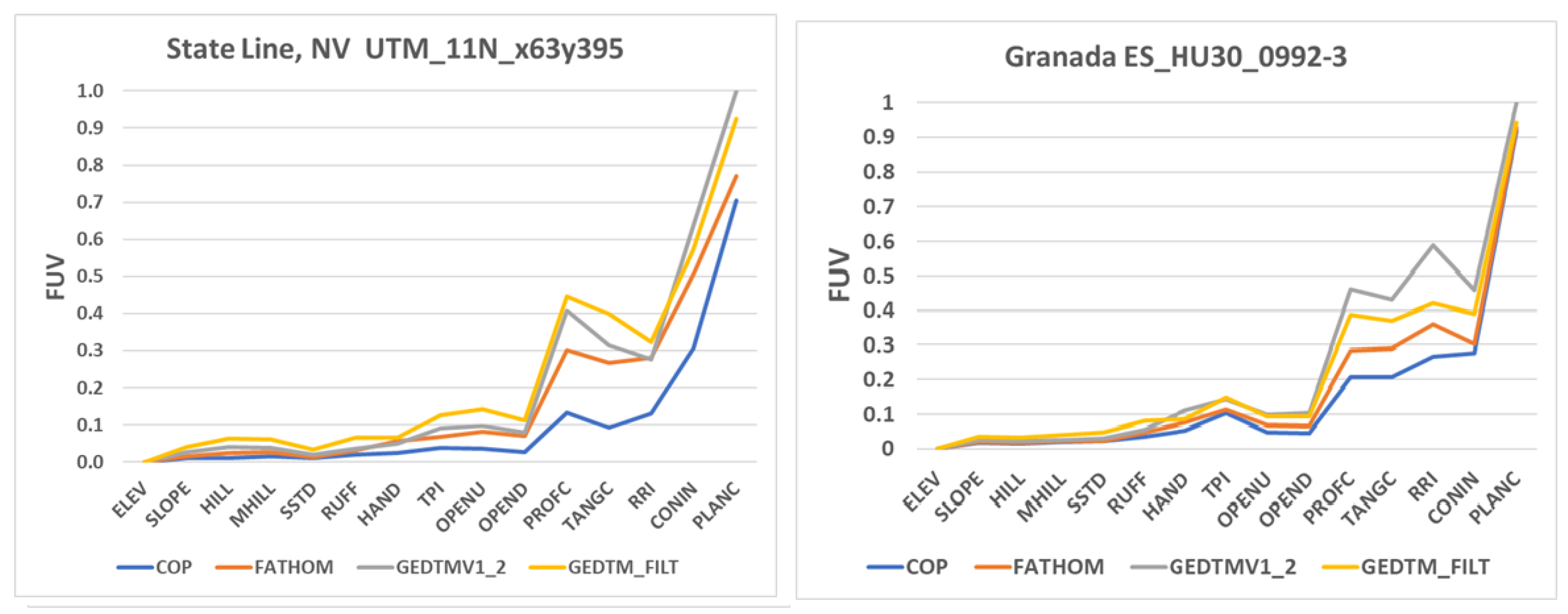
We investigated whether our decision not to filter GEDTM affected our comparisons, using two tiles. We filtered GEDTM with a Gaussian filter from Whitebox [59] using the default parameter (sigma = 0.75) as was done by the GEDTM authors to create their published LSPs [5]. We did not filter the reference DTM or the other test DEMs. The State Line, Nevada, tile has an average slope of 26.85% and is 83.25% barren and was shown in Figure 6, which compares FUV results. The tile in Granada, Spain, has an average slope of 21.55%, and is 46.24% forested and 30.56% barren. The Nevada tile should have needed no corrections to create a DTM, while the Spanish tile’s significant forest cover should have required the removal of vegetation. Figure 23 shows the results. In Nevada, filtering GEDTM led to higher (worse) FUV values, while in Spain it led to higher FUV for the LSPs on the left side of the figure, and better FUV for the LSPs on the right. In each tile, both CopDEM and FathomDEM remained better than GEDTM. Filtering is not a panacea for GEDTM, and the results of filtering appear to depend greatly on the characteristics of the DEM and the particular LSP being calculated.
The progression of the LSPs in our diagrams, from those like slope, which closely match a reference DTM, to those curvature metrics which very poorly match, generally matches the increase in the order of partial derivatives used in the equations. Filtering will smooth and generalize the surface, but the user must carefully decide what is signal and what is noise. Deciding the best step should be the focus of additional research to decide the best approach for different conditions:
  • Filter the DEM before any analysis.
  • Reduce the DEM resolution before analysis, and compute the LSP only on a smaller grid.
  • Filter the LSP after computation.
  • Should all LSPs use the same filter, or should slope be handled differently than change of curvature, since our results indicate that those LSPs have very different characteristics?
  • Do all DEMs require the same filtering?

4.9. Suggestions for DTM Creators

Our results suggest that two of the global one-arc-second DSMs provide the best starting point for edits, CopDEM and ALOS AW3D30. Figure 24 compares them. While the results are not uniform across the five LSP criteria, CopDEM is generally best in tiles with gentler slopes and less barren land; those are categories with the largest number of our test tiles in the lower left portion of the figure. The performance of CopDEM also improves as the overall FUV results decline with more derived LSPs.
Unpacking the effects of the difference between radar (COP) and optical (ALOS) sensors, and then editing DEMs such as Fathom and GEDTM, where the machine learning approaches adopted, and the input features used to improve them vary, becomes a very complex problem. Even just focusing on CopDEM requires a complex analysis [72].
Creators of DTMs using the global one-arc-second DSMs should consider these results and consider different weightings of CopDEM and ALOS when designing their models. DTM creation should also explicitly consider the effect of landcover [72], or our more nuanced depictions of the interplay between slope and landcover (Figure 24).
We think the main improvement of the approach used by FathomDEM is that the convolutional neural network (CNN) approach essentially uses multiscale input features to perform the prediction. In this sense, it performs a “pixel-wise” regression task [19]. But in less exotic terms, CNN applies multiscale filters of the input features, which take into account the surrounding information. With a proper selection of multiscale geomorphometric derivatives, one could obtain similar results by applying a benchmark approach, such as random forest.
DTM validation should also consider the importance of LSPs for many users. Beyond just elevation accuracy, the surface defined by the neighborhood pixels determines LSPs derived from the DEM. There are probably many reasons why FathomDEM outperforms GEDTM, but we feel that Fathom DEM’s use of the slope and roughness LSPs gave it a further advantage in tuning its model, permitting a “pixel-wise” evaluation of accuracy.
As shown earlier, GEDTM outperforms both CopDEM and ALOS in some cases. We hesitate to recommend it for four reasons: (1) download is confusing, and users might inadvertently obtain an undocumented 0.9 arc-second version; (2) versions lacking the vertical scaling factor for elevation are still online and not clearly identified; (3) it performs poorly on many of the LSPs we evaluated; and (4) Fathom DEM clearly outperforms it. Hopefully, the first two issues will be corrected, but the third issue is probably the most important, and we feel that future creation of DTMs should start with CopDEM and ALOS.

4.10. Best DEM Locally or Consistent DEM Globally?

The appeal of the SRTM DEM [73,74] was that for the first time, there was a DEM, collected in a matter of days over most of the earth in a consistent manner. Already at that time, there were better, freely available national DEMs at the same or better spatial resolution (e.g., for the US or Canada [75]), but SRTM allowed comparison of results across the globe. As later versions of SRTM and additional global DEMs have appeared [54,56,76,77], they have borrowed from each other to fill data voids and replace poor quality data.
Later versions of CopDEM used national mapping agency data to infill the DEM in Norway and the Spanish Pyrenees [54]. While this arguably leads to a better product locally, there are questions about whether the infill leads to a DTM or a DSM, but with different characteristics from lidar collection versus the radar collection for the rest of CopDEM. More importantly, why should the infill only apply to those two areas, and not the large number of countries with free high-resolution DEMs (countries in Table 1 and others to include Canada, France, Italy, and Sweden)? The problems with merging the data at national boundaries and adjusting all the DEMs to the same vertical datum are resolvable, but free coverage in much of the world is not likely to be available soon. If Western Europe and North America have a higher quality “global” DEM, slopes computed in the Himalayas or Andes cannot be compared with the Alps or the North American Cordillera because the underlying DEMs have different characteristics.
The USGS evaluated DEMs to use for Landsat orthorectification [78], and chose CopDEM for the next reprocessing. A key factor in that selection was its seamless, global coverage. Our results show that only FathomDEM might be a better choice, and its restrictive license might present issues. Landsat’s optical sensor is probably closer to imaging what a radar DSM sees and not a DTM, and orthorectification probably should use a DSM.

4.11. Future Directions for DEM Comparisons

More one-arc-second DEMs will arrive, from improved sensors and better methods to create DTMs from the DSMs seen from space. For their comparison, we see several ways to improve our methodology.
  • Improve the metrics we use to determine whether our selection of test tiles is representative of the world. There is a wide range of potential data sets classifying geomorphology, climate, and vegetation, and the choice must find a balance between over-specifying categories and generalizing into larger categories. For instance, we could use 14 biomes or 846 ecoregions [79], which have significant implications for how we should select a test area. While every one of the 1.5 million 10 × 10 km areas in the world is unique, we need a much smaller number of categories that we should match.
  • Improve the geographic distribution of our test tiles. The limited number of test tiles in the southern and eastern hemispheres in the earlier versions of our work did not meet the criteria we specified when we redesigned the methodology to use projected national coordinates to define test areas. Hopefully, more lidar-derived DEMs will become available, and we can also investigate if we can relax our criteria. The vertical datum shift was the most restrictive criterion we used, and one way to mitigate its impact would be to use derived LSPs and not consider raw elevation. Not matching the vertical datum does not affect almost all LSPs, which only consider neighborhood elevation differences.
  • To some degree, these improvements are related. If we are confident that we have DEMs in Western Europe or North America that match the characteristics that we think affect the quality of a DEM, then it becomes less important that we have reference DEMs from every region or country. We can reliably measure the global characteristics with satellite data, which effectively covers the world.
  • Consider using landforms to evaluate if our test tiles are representative. The atlas of archetypal landforms [80,81,82] highlights some of the challenges we would see. The atlas has 10 DEMs with resolutions between 0.5 and 10 m, with sizes between 1.5 × 1.5 km and 45 × 45 km, and are coded for 22 different landforms. The extents of the tiles and selected resolution were manually determined by experts. In contrast, our tiles were selected quasi-randomly based on the map tiles distributed by national mapping agencies, and the target scale of the one-arc-second global DEMs we evaluate results in the landscapes appearing very different, and all the tiles are approximately the same size.
  • Two specific landforms show some of the issues we foresee. Karst embodies a number of forms, from sinkholes to cockpit karst with very different geomorphology, and only the largest features will appear at a one-arc-second scale. We could take a map of potential karst in the United States, which has 6 categories [83], to see how many of our tiles could be categorized as karst. This would include the tiles at Mammoth Cave and Puerto Rico, but the vegetation there might be a bigger factor than the karst features apparent with 30 m pixel spacing. Volcanoes might be easier as a landform category, with 1429 Pleistocene and 1232 Holocene volcanoes in the world as picked by experts [84]. With 1.5 million 10 × 10 km tiles in the world, for each age, the probability of a volcano in any given tile would be about one in a thousand (and our sample includes Mount Saint Helens). Is that enough, or should we over-represent volcanoes? Do we need to sample the most common types (shield and strato volcanoes), and do we need multiple examples to trust that the samples are truly representative and not more related to slope or forest cover? Stepping back, how many landforms do we need to cover? Every earth scientist will have favorites; structural geologists might want to see fault block mountains, not included in [80,81,82].
  • Evaluate urban test areas. While we did not actively select urban areas, the urban percentage of our test tiles matches the global distribution. This could result from the size of the tiles, where a few 10 × 10 km tiles will contain only urban 10 m pixels. All of the one-meter DTMs we have seen (the United Kingdom, France, Spain, and the US) have very clear remnants of the roads and building footprints, which clearly survive aggregation to 5 m resolution, and are still visible at 30 m, which decreases our confidence in our urban reference DTMs. Lidar sees the world differently than optical or radar satellite sensors, and reconciling the two is not simple. We think there is more required than simply adding test areas for New York City, Paris, and London. Users of the one-arc-second DEMs in urban areas need to consider their purpose and the appropriateness of one-arc-second data.
  • Evaluate tiles with tropical forests, for which we should be able to find test areas, and keep looking for desert areas in the great belt from North Africa through the Middle East into Central Asia. We already have some desert areas (e.g., Colorado’s Great Sand Dune, but they lack the great dune fields where a DSM and DTM should be identical. Users who want guidance on the best global DEM to use in those cases must use our general guidance and determine which DEM would be best in their circumstances.
  • Investigate alternative aggregation methods to create the reference one-arc-second reference DTM from the one-meter source DTMs. Our current method uses mean aggregation, effectively mean filtering over an irregular rectangular window, and we might use the median, or a weighted function that places more weight on the central point.
  • Investigate the need for filtering before creating LSPs. The recommendations to filter first are several decades old, when DEMs had only a meter vertical resolution and were created with very different technology. We see three questions that further research should resolve: (1) should all DEMs be filtered; (2) should the producer or user do the filtering; and (3) what filter should be used.

5. Conclusions

Comparisons of global DEMs should use multiple criteria from different LSPs. These use all points in the DEM, and better represent the many different uses of DEMs. Creators of DTMs should use multiple LSPs to assess and improve their processing flow.
Many LSPs commonly used in geomorphometry do a poor job with the global DEMs matching calculations from a reference DTM at the same resolution. In particular, this is true for many of the curvature measures, especially those using third-order partial derivatives. LSP performance occurs on a continuum, and the decision on which LSPs perform acceptably remains a subjective decision.
FathomDEM is currently the best one-arc-second DTM. If users cannot accept its restrictive license, they should use CopDEM. Even if it is a DSM, it outperforms the unrestricted GEDTM compared to a reference DTM. If the usage is only in steep, mountainous areas, ALOS would be the best choice.
Great care should be taken when using GEDTM version 1.2, and especially its precomputed LSPs. GEDTM does a poor job with derived LSPs, and users must be careful to ensure they have the one-arc-second version and that it has the correct scaling factor to adjust its decimeter elevations. Users should carefully consider the metadata that should accompany DEM data. GEDTM is the only one of the edited DTMs that published its scripts, so that users can follow the processing steps even if there is no kind of metadata available with CopDEM, which shows the origin of every edited pixel in the final DEM.
Future work creating DTMs should consider starting with CopDEM, but using ALOS AW3D30 for steep areas where it performs better. In steep areas the integer precision of AW3D30 has less impact on the results, and the optical sensor probably also outperforms radar.
Our test tiles do not include major urban areas, dense tropical forests, or major deserts, which represent very complex regions for global DEMs. Our results might not apply in those regions where obtaining reference DTMs creates huge challenges.

Author Contributions

Conceptualization, P.L.G., S.T., C.H.G., J.B.L. and H.I.R.; methodology, P.L.G.; software, P.L.G.; validation, P.L.G.; formal analysis, P.L.G.; investigation, P.L.G.; resources, P.L.G.; data curation, P.L.G.; writing—original draft preparation, P.L.G.; writing—review and editing, P.L.G., S.T., C.H.G., J.B.L. and H.I.R.; visualization, P.L.G. All authors have read and agreed to the published version of the manuscript.

Funding

C.H.G. is supported by The São Paulo Research Foundation (FAPESP—grant #2023/11197-1) and CNPq (grant #300033/2025-7). J.B.L. is funded by a Natural Sciences and Engineering Research Council of Canada (NSERC) grant number 401107.

Data Availability Statement

High resolution DEMs are available in the national repositories listed in Table 1, and ref. [51] lists the source files used for each test tile. The global one-arc-second DEMs are available online: CopDEM [55], FABDEM with license [4], FathomDEM with license [20,21], ALOS AW3D30 [56], EDTM [52], and GEDTM [22,23,24]. The database tables with our results are available [26,51].

Acknowledgments

We thank our colleagues in the initial DEMIX papers [18,25] for many online discussions over the years that got us started on this work. The work would not be possible without the work of the many national mapping agencies that post their DEMs, the space agencies that have created the global one-arc-second DEMs, and the groups that have attempted to create DTMs from DSMs.

Conflicts of Interest

Three of the authors (C.H.G., J.B.L. and H.I.R.) were also involved with creation of GEDTM [5]. That did not influence our evaluation of GEDTM, which is not, in fact, very positive. The authors declare that the research was conducted in the absence of any commercial or financial relationships that could be construed as a potential conflict of interest.

Abbreviations

The following abbreviations are used in this manuscript:
ALOSAW3D30 DEM
COP, CopDEMCopernicus DEM
DEMDigital elevation model
DEMIXDigital Elevation Model Intercomparison Exercise
DSMDigital surface model
DTMDigital surface model
FUVFraction of unexplained variance
GNSSGlobal navigation satellite system
LE90Linear error 90th percentile
LSPLand surface parameter
MAEMean average error
RMSERoot mean square error
USGSUnited States Geological Survey

References

  1. Guth, P.L.; Van Niekerk, A.; Grohmann, C.H.; Muller, J.P.; Hawker, L.; Florinsky, I.V.; Gesch, D.; Reuter, H.I.; Herrera-Cruz, V.; Riazanoff, S.; et al. Digital Elevation Models: Terminology and Definitions. Remote Sens. 2021, 13, 3581. [Google Scholar] [CrossRef]
  2. O’Loughlin, F.; Paiva, R.; Durand, M.; Alsdorf, D.; Bates, P. A multi-sensor approach towards a global vegetation corrected SRTM DEM product. Remote Sens. Environ. 2016, 182, 49–59. [Google Scholar] [CrossRef]
  3. Yamazaki, D.; Ikeshima, D.; Tawatari, R.; Yamaguchi, T.; O’Loughlin, F.; Neal, J.C.; Sampson, C.C.; Kanae, S.; Bates, P.D. A high-accuracy map of global terrain elevations. Geophys. Res. Lett. 2017, 44, 5844–5853. [Google Scholar] [CrossRef]
  4. Hawker, L.; Uhe, P.; Paulo, L.; Sosa, J.; Savage, J.; Sampson, C.; Neal, J. A 30 m global map of elevation with forests and buildings removed. Environ. Res. Lett. 2022, 17, 024016. [Google Scholar] [CrossRef]
  5. Ho, Y.F.; Grohmann, C.; Lindsay, J.; Reuter, H.; Parente, L.; Witjes, M.; Hengl, T. GEDTM30: Global ensemble digital terrain model at 30 m and derived multiscale terrain variables. PeerJ 2025, 13, e19673. [Google Scholar] [CrossRef]
  6. Blewitt, G.; Hammond, W.; Kreemer, C. Harnessing the GPS data explosion for interdisciplinary science. Eos 2018, 99, e2020943118. [Google Scholar] [CrossRef]
  7. Nevada Geodetic Laboratory. Space Reference Points (SRPs). Available online: https://geodesy.unr.edu/gps_timeseries/IGS20/llh/llh.out (accessed on 6 November 2025).
  8. Han, M.; Enwright, N.M.; Gesch, D.B.; Stoker, J.; Danielson, J.J.; Amante, C.J. Contractor Vertical Accuracy Checkpoints for 3D Elevation Program Digital Elevation Models in the Northern Gulf of Mexico and Atlantic Coastal Regions, 2012–2020; U.S. Geological Survey: Reston, VA, USA, 2024; Volume 751. Available online: https://data.usgs.gov/datacatalog/data/USGS:64b8833ed34e70357a2b56a0 (accessed on 26 November 2025).
  9. Han, M.; Enwright, N.M.; Gesch, D.B.; Stoker, J.M.; Danielson, J.J.; Amante, C.J. Assessing the vertical accuracy of digital elevation models by quality level and land cover. Remote Sens. Lett. 2024, 15, 667–677. [Google Scholar] [CrossRef]
  10. AIRBUS. Space Reference Points (SRPs). Available online: https://space-solutions.airbus.com/imagery/3d-elevation-and-reference-points/srp/ (accessed on 26 November 2025).
  11. Zhu, X.; Nie, S.; Zhu, Y.; Chen, Y.; Yang, B.; Li, W. Evaluation and Comparison of ICESat-2 and GEDI Data for Terrain and Canopy Height Retrievals in Short-Stature Vegetation. Remote Sens. 2023, 15, 4969. [Google Scholar] [CrossRef]
  12. Tian, X.; Shan, J. Comprehensive evaluation of the ICESat-2 ATL08 terrain product. IEEE Trans. Geosci. Remote Sens. 2021, 59, 8195–8209. [Google Scholar] [CrossRef]
  13. Li, H.; Zhao, J.; Yan, B.; Yue, L.; Wang, L. Global DEMs vary from one to another: An evaluation of newly released Copernicus, NASA and AW3D30 DEM on selected terrains of China using ICESat-2 altimetry data. Int. J. Digit. Earth 2022, 15, 1149–1168. [Google Scholar] [CrossRef]
  14. Pracná, P.; Šárovcová, E.; Liu, X.; Eltner, A.; Marešová, J.; Gdulová, K.; Urbazaev, M.; Torresani, M.; Kozhoridze, G.; Moudrý, V. Towards 90 m resolution Digital Terrain Model combining ICESat-2 and GEDI data: Balancing Accuracy and Sampling Intensity. Sci. Remote Sens. 2025, 12, 100293. [Google Scholar] [CrossRef]
  15. University of Washington; NASA Goddard Space Flight Center. SlideRule. Available online: https://client.slideruleearth.io/ (accessed on 10 November 2025).
  16. NASA National Snow and Ice Data Center Distributed Active Archive Center. OpenAltimetry. Available online: https://openaltimetry.earthdatacloud.nasa.gov/data/ (accessed on 10 November 2025).
  17. Guth, P.L.; Geoffroy, T.M. LiDAR point cloud and ICESat-2 evaluation of 1 second global digital elevation models: Copernicus wins. Trans. GIS 2021, 2245–2261. [Google Scholar] [CrossRef]
  18. Bielski, C.; López-Vázquez, C.; Grohmann, C.; Guth, P.; Hawker, L.; Gesch, D.; Trevisani, S.; Herrera-Cruz, V.; Riazanoff, S.; Corseaux, A.; et al. Novel Approach for Ranking DEMs: Copernicus DEM Improves One Arc Second Open Global Topography. IEEE Trans. Geosci. Remote Sens. 2024, 62, 1–22. [Google Scholar] [CrossRef]
  19. Uhe, P.; Lucas, C.; Hawker, L.; Brine, M.; Wilkinson, H.; Cooper, A.; Saoulis, A.A.; Savage, J.; Sampson, C. FathomDEM: An improved global terrain map using a hybrid vision transformer model. Environ. Res. Lett. 2025, 20, 034002. [Google Scholar] [CrossRef]
  20. Fathom (United Kingdom). FathomDEM v1-0 Americas. 2024. Available online: https://zenodo.org/records/14523356 (accessed on 26 November 2025).
  21. Fathom (United Kingdom). FathomDEM v1-0 Eurasia and Africa. 2024. Available online: https://zenodo.org/records/14511570 (accessed on 26 November 2025).
  22. Ho, Y.F.; Hengl, T. Global Ensemble Digital Terrain Model 30 m (GEDTM30) (Version 0) [Data Set]. 2025. Available online: https://zenodo.org/records/14900181 (accessed on 26 November 2025).
  23. Ho, Y.F.; Hengl, T. Global Ensemble Digital Terrain Model 30 m (GEDTM30) (Version 1.1) [Data Set]. 2025. Available online: https://zenodo.org/records/15689805 (accessed on 26 November 2025).
  24. Ho, Y.F. GEDTM30. Available online: https://s3.opengeohub.org/global/dtm/v1.2/gedtm_rf_m_30m_s_20060101_20151231_go_epsg.4326.3855_v1.2.tif (accessed on 16 September 2025).
  25. Guth, P.L.; Trevisani, S.; Grohmann, C.H.; Lindsay, J.; Gesch, D.; Hawker, L.; Bielski, C. Ranking of 10 Global One-Arc-Second DEMs Reveals Limitations in Terrain Morphology Representation. Remote Sens. 2024, 16, 3273. [Google Scholar] [CrossRef]
  26. Guth, P.L. DEMIX GIS Database Version 3.5 [Data Set]. 2025. Available online: https://zenodo.org/records/17247343 (accessed on 26 November 2025).
  27. Guth, P.L.; Strobl, P.; Gross, K.; Riazanoff, S. DEMIX 10k Tile Data Set (1.0). Dataset on Zenodo. 2023. Available online: https://zenodo.org/records/7504791 (accessed on 26 November 2025).
  28. GDAL/OGR Contributors. GDAL/OGR Geospatial Data Abstraction Software Library. Open Source Geospatial Foundation. 2025. Available online: https://gdal.org/en/stable/ (accessed on 26 November 2025).
  29. Centro Nacional de Información Geográfica (Spain). Download Center. Available online: https://centrodedescargas.cnig.es/CentroDescargas/buscar-mapa (accessed on 15 August 2025).
  30. Danish Climate Data Agency. Denmark’s Elevation Model—Terrain. Available online: https://dataforsyningen.dk/data/930 (accessed on 28 September 2025).
  31. Land and Spatial Development Board. Elevation Data Map Sheet Query. Available online: https://geoportaal.maaamet.ee/eng/spatial-data/elevation-data/download-elevation-data-p664.html (accessed on 22 August 2025).
  32. National Land Survey of Finland. Elevation Model. Available online: https://asiointi.maanmittauslaitos.fi/karttapaikka/tiedostopalvelu/korkeusmalli?lang=en (accessed on 22 August 2025).
  33. State Office for Geoinformation Saxony. Batch Download. Available online: https://www.geodaten.sachsen.de/batch-download-4719.html (accessed on 21 August 2025).
  34. Bavarian Surveying Authority. Digital Terrain Model 1 m (DGM1). Available online: https://geodaten.bayern.de/opengeodata/OpenDataDetail.html?pn=dgm1 (accessed on 21 August 2025).
  35. The Surveying and Cadastral Administration of Rhineland-Palatinate. Digital Terrain Model Grid Spacing 1 m. Available online: https://geoshop.rlp.de/opendata-dgm1.html (accessed on 21 August 2025).
  36. INEGI. Continental Relief. Available online: https://www.inegi.org.mx/temas/relieve/continental/ (accessed on 13 August 2025).
  37. Actueel Hoogtebestand Nederland (AHN). Data Feed—Digital Terrain Model (DTM) 0.5 m. Available online: https://service.pdok.nl/rws/ahn/atom/dtm_05m.xml (accessed on 18 August 2025).
  38. Federal Office of Topography Surveys Switzerland. swissALTI3D—Download. Available online: https://www.swisstopo.admin.ch/de/hoehenmodell-swissalti3d#swissALTI3D—Download (accessed on 13 August 2025).
  39. Department for Environment. Defra Survey Data Download. Available online: https://environment.data.gov.uk/survey (accessed on 26 November 2025).
  40. Scottish Government. Scottish Remote Sensing Portal. Available online: https://remotesensingdata.gov.scot/data#/map (accessed on 13 August 2025).
  41. United States Geological Survey. TNM Download (v2.0). Available online: https://apps.nationalmap.gov/downloader/ (accessed on 19 July 2025).
  42. Guth, P.L. prof-pguth-git_microdem. Available online: https://github.com/prof-pguth/git_microdem (accessed on 10 July 2025).
  43. Zanaga, D.; Van De Kerchove, R.; Daems, D.; De Keersmaecker, W.; Brockmann, C.; Kirches, G.; Wevers, J.; Cartus, O.; Santoro, M.; Fritz, S.; et al. ESA WorldCover 10 m 2021 v200 (Version v200) [Data Set]. 2022. Available online: https://zenodo.org/records/7254221 (accessed on 26 November 2025).
  44. Buchhorn, M.; Smets, B.; Bertels, L.; Roo, B.D.; Lesiv, M.; Tsendbazar, N.E.; Herold, M.; Fritz, S. Copernicus Global Land Service: Land Cover 100 m: Collection 3: Epoch 2019: Globe. 2020. Available online: https://zenodo.org/records/3939050 (accessed on 26 November 2025).
  45. Feciskanin, R.; Hajdúchová, V. New Tool for Calculating Land Surface Parameters. Zenodo. 2025. Available online: https://zenodo.org/records/15005370 (accessed on 26 November 2025).
  46. Feciskanin, R. Land Surface Parameters Calculator. Available online: https://github.com/xiceph/physical-geomorphometry-tools/tree/main/lsp-calculator (accessed on 10 July 2025).
  47. Guth, P.L. MICRODEM: Open-Source GIS with a Focus on Geomorphometry. Available online: https://microdem.org/ (accessed on 10 July 2025).
  48. Minár, J.; Evans, I.S.; Jenčo, M. A comprehensive system of definitions of land surface (topographic) curvatures, with implications for their application in geoscience modelling and prediction. Earth-Sci. Rev. 2020, 211, 103414. [Google Scholar] [CrossRef]
  49. Guth, P.L. DEMIX GIS Database (3.0). 2024. Available online: https://zenodo.org/records/13331458 (accessed on 26 November 2025).
  50. Guth, P.L. DEMIX GIS Database Version 2. 2023. Available online: https://zenodo.org/records/8062008 (accessed on 26 November 2025).
  51. Guth, P.L. DEMIX GIS Database Version 4 [Data Set]. 2025. Available online: https://zenodo.org/records/17538186 (accessed on 26 November 2025).
  52. Ho, Y.F.; Hengl, T.; Leandro, P. Ensemble Digital Terrain Model (EDTM) of the World (1.1) [Data Set]. 2023. Available online: https://zenodo.org/records/7676373 (accessed on 26 November 2025).
  53. Ho, Y.F.; Hengl, T.; Parente, L. An Ensemble Digital Terrain Model of the World at 30 m Spatial Resolution (EDTM30) on Medium. Medium. 2023. Available online: https://medium.com/nerd-for-tech/an-ensemble-digital-terrain-model-of-the-world-at-30-m-spatial-resolution-edtm30-b4fcff38164c (accessed on 26 November 2025).
  54. AIRBUS Defence and Space. Copernicus DEM Product Handbook Version 5. Available online: https://dataspace.copernicus.eu/sites/default/files/media/files/2024-06/geo1988-copernicusdem-spe-002_producthandbook_i5.0.pdf (accessed on 26 November 2025).
  55. Access to Copernicus Digital Elevation Model (DEM). Available online: https://explore.creodias.eu/ (accessed on 6 November 2025).
  56. Precise Global Digital 3D Map “ALOS World 3D” Homepage. Available online: https://www.eorc.jaxa.jp/ALOS/en/dataset/aw3d30/aw3d30_e.htm (accessed on 10 July 2025).
  57. Tadono, T.; Nagai, H.; Ishida, H.; Oda, F.; Naito, S.; Minakawa, K.; Iwamoto, H. Generation of the 30 M-Mesh Global Digital Surface Model by ALOS PRISM. Int. Arch. Photogramm. Remote Sens. Spat. Inf. Sci. 2016, XLI-B4, 157–162. [Google Scholar] [CrossRef]
  58. Neal, J.; Hawker, L. FABDEM V1-2. 2023. Available online: https://data.bris.ac.uk/data/dataset/s5hqmjcdj8yo2ibzi9b4ew3sn (accessed on 26 November 2025).
  59. Whitebox Software. Available online: https://www.whiteboxgeo.com/ (accessed on 13 November 2025).
  60. Welcome to the SAGA Homepage. Available online: https://saga-gis.sourceforge.io/en/index.html (accessed on 13 June 2024).
  61. Grohmann, C.H.; Smith, M.J.; Riccomini, C. Multiscale Analysis of Topographic Surface Roughness in the Midland Valley, Scotland. IEEE Trans. Geosci. Remote Sens. 2011, 49, 1200–1213. [Google Scholar] [CrossRef]
  62. Yokoyama, R.; Shirasawa, M.; Pike, R.J. Visualizing topography by openness: A new application of image processing to digital elevation models. Photogramm. Eng. Remote Sens. 2002, 68, 257–266. [Google Scholar]
  63. Olaya, V. Chapter 6 Basic Land-Surface Parameters. In Developments in Soil Science; Hengl, T., Reuter, H.I., Eds.; Elsevier: Amsterdam, The Netherlands, 2009; Volume 33, pp. 141–169. [Google Scholar] [CrossRef]
  64. Wilson, J.P. Digital terrain modeling. Geomorphology 2012, 137, 107–121. [Google Scholar] [CrossRef]
  65. Minár, J.; Drăguţ, L.; Evans, I.S.; Feciskanin, R.; Gallay, M.; Jenčo, M.; Popov, A. Physical geomorphometry for elementary land surface segmentation and digital geomorphological mapping. Earth-Sci. Rev. 2024, 248, 104631. [Google Scholar] [CrossRef]
  66. Meadows, M.; Jones, S.; Reinke, K. Vertical accuracy assessment of freely available global DEMs (FABDEM, Copernicus DEM, NASADEM, AW3D30 and SRTM) in flood-prone environments. Int. J. Digit. Earth 2024, 17, 2308734. [Google Scholar] [CrossRef]
  67. Trevisani, S.; Skrypitsyna, T.; Florinsky, I. Global digital elevation models for terrain morphology analysis in mountain environments: Insights on Copernicus GLO-30 and ALOS AW3D30 for a large Alpine area. Environ. Earth Sci. 2023, 82, 198. [Google Scholar] [CrossRef]
  68. Shary, P.A.; Sharaya, L.S.; Mitusov, A.V. Fundamental quantitative methods of land surface analysis. Geoderma 2002, 107, 1–32. [Google Scholar] [CrossRef]
  69. Reuter, H.; Hengl, T.; Gessler, P.; Soille, P. Preparation of DEMs for geomorphometric analysis. Dev. Soil Sci. 2009, 33, 87–120. [Google Scholar] [CrossRef]
  70. Florinsky, I.V. Computation of the third-order partial derivatives from a digital elevation model. Int. J. Geogr. Inf. Sci. 2009, 23, 213–231. [Google Scholar] [CrossRef]
  71. Callow, J.N.; Van Niel, K.P.; Boggs, G.S. How does modifying a DEM to reflect known hydrology affect subsequent terrain analysis? J. Hydrol. 2007, 332, 30–39. [Google Scholar] [CrossRef]
  72. Meadows, M.; Reinke, K.; Jones, S. Explaining machine learning models trained to predict Copernicus DEM errors in different land cover environments. Artif. Intell. Geosci. 2025, 6, 100141. [Google Scholar] [CrossRef]
  73. USGS EROS Archive—Digital Elevation—Shuttle Radar Topography Mission (SRTM) 1 Arc-Second Global. Available online: https://www.usgs.gov/centers/eros/science/usgs-eros-archive-digital-elevation-shuttle-radar-topography-mission-srtm-1-arc?qt-science_center_objects=0#qt-science_center_object (accessed on 19 July 2021).
  74. Rodriguez, E.; Morris, C.H.; Belz, J.E. A global assessment of the SRTM performance. Photogramm. Eng. Remote Sens. 2006, 72, 249–260. [Google Scholar] [CrossRef]
  75. Guth, P.L. Geomorphometry from SRTM: Comparison to NED. Photogramm. Eng. Remote Sens. 2006, 72, 269–278. [Google Scholar] [CrossRef]
  76. Abrams, M.; Crippen, R.; Fujisada, H. ASTER Global Digital Elevation Model (GDEM) and ASTER Global Water Body Dataset (ASTWBD). Remote Sens. 2020, 12, 1156. [Google Scholar] [CrossRef]
  77. NASA JPL. NASA SRTM-Only Height and Height Precision Global 1 Arc Second V001. Distributed by NASA EOSDIS Land Processes DAAC. 2020. Available online: https://www.earthdata.nasa.gov/data/catalog/lpcloud-nasadem-shhp-001 (accessed on 26 November 2025).
  78. Franks, S.; Rengarajan, R. Evaluation of Copernicus DEM and Comparison to the DEM Used for Landsat Collection-2 Processing. Remote Sens. 2023, 15, 2509. [Google Scholar] [CrossRef]
  79. Dinerstein, E.; Olson, D.; Joshi, A.; Vynne, C.; Burgess, N.D.; Wikramanayake, E.; Hahn, N.; Palminteri, S.; Hedao, P.; Noss, R.; et al. An Ecoregion-Based Approach to Protecting Half the Terrestrial Realm. BioScience 2017, 67, 534–545. [Google Scholar] [CrossRef]
  80. Kennelly, P.J.; Patterson, T.; Jenny, B.; Huffman, D.P.; Marston, B.E.; Bell, S.; Tait, A.M. Elevation models for reproducible evaluation of terrain representation. Cartogr. Geogr. Inf. Sci. 2021, 48, 63–77. [Google Scholar] [CrossRef]
  81. Kennelly, P.J.; Patterson, T.; Jenny, B.; Huffman, D.P.; Marston, B.E.; Bell, S.; Tait, A.M. Elevation Models for Reproducible Evaluation of Terrain Representation—Archetypal Landforms [Data Set Version 2.0]. Dataset on Zenodo. 2020. Available online: https://zenodo.org/records/4323616 (accessed on 26 November 2025).
  82. Kennelly, P.J.; Patterson, T.; Jenny, B.; Huffman, D.P.; Marston, B.E.; Bell, S.; Tait, A.M. Sample Elevation Models for Evaluating Terrain Representation. Available online: https://shadedrelief.com/SampleElevationModels/ (accessed on 12 November 2025).
  83. Weary, D.; Doctor, D. Karst in the United States: A Digital Map Compilation and Database; Open-File Report 2014-1156; U.S. Geological Survey: Reston, VA, USA, 2014. [Google Scholar] [CrossRef]
  84. Distributed by Smithsonian Institution, Compiled by Venzke, E. Volcanoes of the World (Database v. 5.3.2; 30 Sep 2025). Available online: https://volcano.si.edu/gvp_votw.cfm (accessed on 12 November 2025).
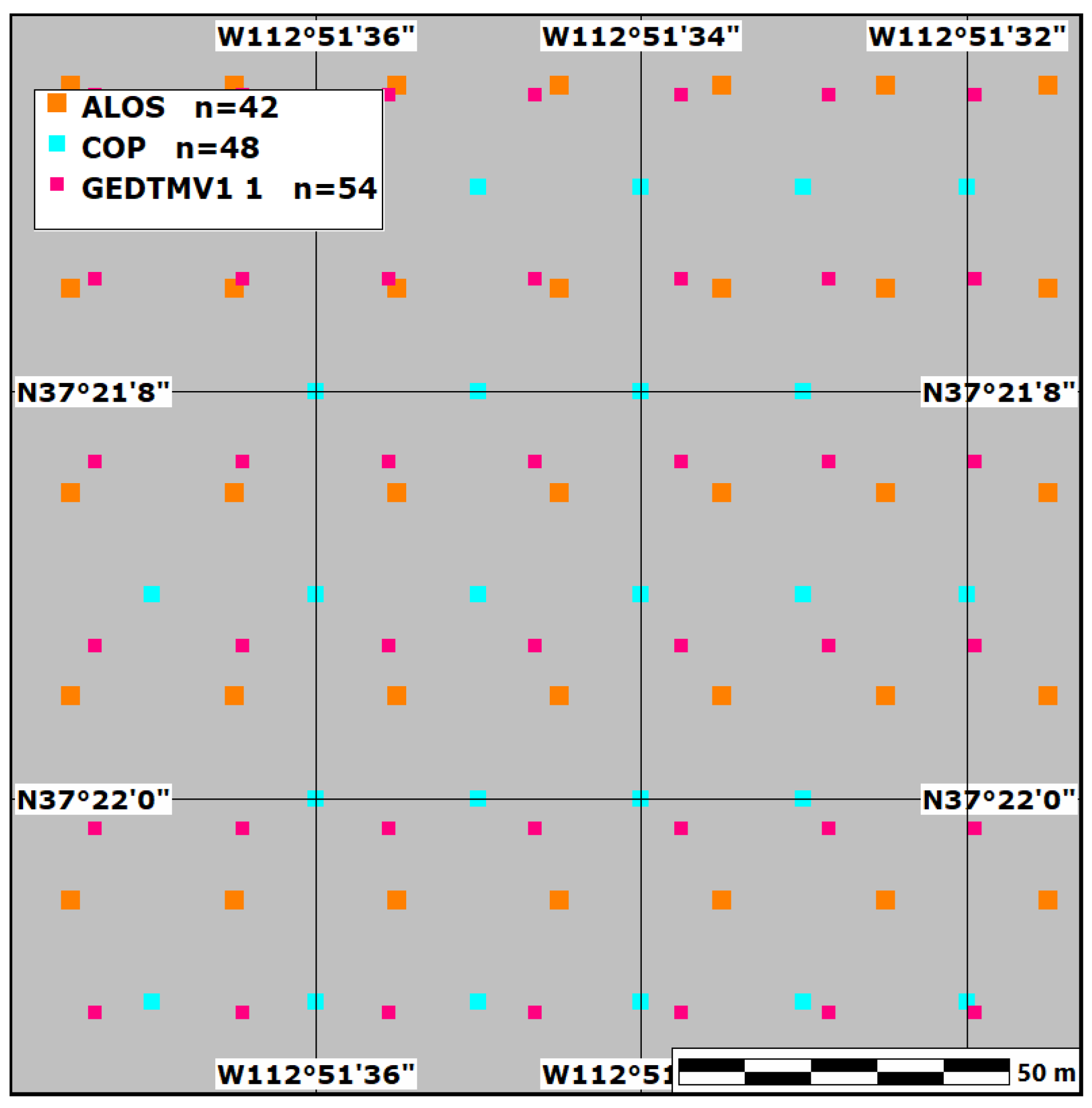
Figure 1. Pixel geometry models for the DEMs considered in this paper. The ALOS and SRTM pixel locations models have a consistent half-pixel offset, while the GEDTM model used in some versions of their DTM migrates in relation to the others due to its smaller pixel spacing.
Remotesensing 17 03919 g001
Figure 2. Average slope for the tiles in our database, for the reference DTM in three pixel geometry models. Averages for the SRTM and ALOS models are essentially identical, but the GEDTM slopes are consistently higher due to the smaller data spacing. All r2 values are very close to 1.
Remotesensing 17 03919 g002
Figure 3. CopDEM has better FUV and wins compared to SRTM, ASTER GDEM, NASADEM, and TANDEM-X except in the low slope, low barrenness bin where NASADEM has a slight advantage. Data from [49].
Remotesensing 17 03919 g003
Figure 4. Locations in red for the test areas for evaluations and coast lines in blue.
Remotesensing 17 03919 g004
Figure 5. Percentage of tiles in 18 terrain bins based on average tile slope and the percentage of the tile that is barren, (a) show the relative percentages in each bin with the world distribution in blue, (b) emphasize where our databases overemphasize bins compared to the world distribution of tiles in blue, an (c) emphasize where our databases are under-represented compared to the world distribution of tiles in blue.
Remotesensing 17 03919 g005
Figure 6. Scatter plot for 5 criteria, comparing CopDEM and GEDTM with the reference DTM. FUV and r2 value shown in the upper left corner.
Remotesensing 17 03919 g006
Figure 7. The top row shows the best evaluation among all test DEMs for all LSPs used as criteria for four slope categories, while the bottom row shows the five criteria we highlight the range of LSP sensitivity.
Remotesensing 17 03919 g007
Figure 8. FUV versus best evaluation for any of the four test DEMs in the columns and five LSP criteria in the rows. Gray dots show all DEMs.
Remotesensing 17 03919 g008
Figure 9. FUVs sorted by average tile slope, with 4 test DEMs in the columns and 5 LSP criteria in the rows. Gray dots show all the DEMs.
Remotesensing 17 03919 g009
Figure 10. FUVs sorted by average tile barren percentage, with 4 test DEMs in the columns and 5 LSP criteria in the rows. Gray dots show all the DEMs.
Remotesensing 17 03919 g010
Figure 11. Criterion average FUV versus tile characteristics. Five criteria in the columns, and five terrain characteristics in the rows. The horizontal axis shows the full 0–1 range for each graph to emphasize the differences among the criteria. Some spikes may reflect very small sample sizes.
Remotesensing 17 03919 g011
Figure 12. Criterion average FUV versus tile characteristics. Five criteria in the columns, and five terrain characteristics in the rows. The horizontal axis is stretched differently for each graph to emphasize the differences among the test DEMs in the different terrain categories.
Remotesensing 17 03919 g012
Figure 13. FUV on the vertical axis versus criteria on the horizontal axis, for combinations of average tile slope (rows) and percentage barenness (columns) tile characteristics. Colored lines show the test DEMs.
Remotesensing 17 03919 g013
Figure 14. FUV on the vertical axis versus partial derivative criteria on the horizontal axis, for nine combinations of slope and barenness tile characteristics. Colored lines show the test DEMs.
Remotesensing 17 03919 g014
Figure 15. FUV on the vertical axis versus curvature criteria on the horizontal axis, for nine combinations of slope and barenness tile characteristics. Colored lines show the test DEMs.
Remotesensing 17 03919 g015
Figure 16. Comparison of FUV for four curvature measures computed with two algorithms: the traditional Evans and LSPcalc methods. The four measures from left (best) to right (worst) are SLOPE, PROFC/KNS, and TANGC/KNC, which are similar, and PLANC/KPC.
Remotesensing 17 03919 g016
Figure 17. RMSE for 5 DEMs for the elevation, slope, and roughness (standard deviation of slope) difference distributions. Gray dots show all DEMs.
Remotesensing 17 03919 g017
Figure 18. Best DEM considering the mixed LSP criteria and four slope categories. The panel on top shows all five DEMs we consider, and the bottom panel only those with an unrestricted license.
Remotesensing 17 03919 g018
Figure 19. Best test DEM for the four DEMs considered (top row) and the three DEMs with unrestricted licenses (bottom row). This uses RMSE for the elevation, slope, and roughness difference distributions, with 16 slope and roughness categories.
Remotesensing 17 03919 g019
Figure 20. Best DEM among the four considered DEMs (top row) and the three unrestricted DEMs (bottom row) for all of the grids computed for partial derivatives. Each graph has a grid with 16 pie diagrams for slope and barrenness categories.
Remotesensing 17 03919 g020
Figure 21. Pie diagrams showing the best among all four test DEMs (top row) and the three with unrestricted licenses (bottom row) for five curvature LSPs.
Remotesensing 17 03919 g021
Figure 22. Comparison of the best DEM considering CopDEM, EDTM, and three versions of GEDTM for three LSPs. Data from [26].
Remotesensing 17 03919 g022
Figure 23. Results from filtering GEDTM before computing LSPs for two tiles.
Remotesensing 17 03919 g023
Figure 24. Best test DEM considering CopDEM, ALOS AW3D30, and GEDTM for 5 LSP criteria considering both slope and landcover.
Remotesensing 17 03919 g024
Table 1. Characteristics of source national DEM tiles used to create UTM DEMIX tiles.
CountryResolution (m)Tile GeometryMerged TilesHorizontal DatumVertical Datum (EPSG)Tile Size (km)Download
Canary Islands2Quarter MTN25 map sheet1ETRS89 UTM939716.9 × 10.0 [29]
Denmark0.4UTM 1 × 1 km in 10 × 10 km zip100ETRS89 UTM579910 × 10 [30]
Estonia15 × 5 km 1:10 K quarter map sheets433019663 (no GDAL support)10 × 10 [31]
Finland2UTM 6 × 6 km TM35 map divisions4ETRS89 UTM390012 × 12 [32]
Germany (by State)1UTM 1 × 1 km100ETRS89 UTM783710 × 10 [33,34,35]
Mexico1.5Quarter 1:10 K map sheets4NAD83 UTM570310.6 × 14.0 [36]
Netherlands0.5Quarter map sheet4EPSG 28992573010.0 × 12.5 [37]
Spain2Quarter MTN25 map sheet1ETRS89 UTM578214.7 × 9.7 [29]
Switzerland2Swiss grid 1 × 1 km100EPSG 2056572810 × 10 [38]
UK (England, Scotland)1OSGB Quarter 10 km4EPSG 27700570110 × 10 [39,40]
USA1UTM 10 × 10 km1NAD83 UTM570310 × 10 [41]
Table 3. Test DEMs used in comparison.
DEMLicensePixel GeometrySource DataDTM Edit MethodsReferences
CopDEM v2023-1 (DSM)FreeSRTMRadarNone (DSM) [54,55]
AW3D30 v3.2 (DSM)FreeALOSOpticalNone (DSM) [56,57]
FABDEM v1.2 (DSM)RestrictiveSRTMRadarRandom forest [4,58]
Fathom v1 DTMRestrictiveSRTMRadarHybrid vision transformer model [19,20,21]
GEDTM v1.2FreeSRTMRadarTwo-stage random forest model [5,22,23,24]
Table 4. Criteria based on comparing every pixel in grids.
CriterionNameUnitsAlgorithmWindowProgramTolerance
ELEVElevationMeterDirectly from test DEM 0.0001
HILLHillshade 3 × 3MICRODEM0.005
MHILLMultidirectional hillshade 3 × 3Whitebox0.005
SLOPESlopePercentEvans3 × 3MICRODEM0.02
SSTDSpherical StdDev Of Normals 5 × 5Whitebox0.01
RUFFRoughnessPercentStd slope [61]5 × 5MICRODEM0.01
TPITopographic position indexmeter 3 × 3MICRODEM0.01
HANDHeight above nearest drainageMeter Whitebox0.05
OPENUUpward OpennessDegree [62]11 × 11MICRODEM0.005
OPENDDownward OpennessDegree [62]11 × 11MICRODEM0.005
TANGCTangential curvatureper meter 3 × 3Whitebox0.0001
PROFCProfile curvatureper meter 3 × 3Whitebox0.0001
RRIRadial roughness indexmeter 5 × 5MICRODEM0.015
CONINConvergence indexdegrees SAGA0.01
PLANCPlan curvatureper meter 3 × 3Whitebox0.000025
Table 5. Partial derivative criteria and the tolerances used for ties.
CriterionNameTolerance
ELEVElevation0.0001
Z_FITFitted elevation0.0001
ZXFirst order derivative0.001
ZYFirst order derivative0.001
ZXXSecond order derivative0.001
ZXYSecond order mixed derivative0.001
ZYYSecond order derivative0.001
ZXXXThird order derivative0.001
ZXXYThird order mixed derivative0.001
ZXYYThird order mixed derivative0.001
ZYYYThird order derivative0.001
Table 6. Curvature criteria and tolerances used for ties.
CriterionNamePartial OrderUnitsTolerance
ELEVElevation0m0.0001
SLOPEslope1Degree0.0001
COS-Acosine aspect1none0.0001
SIN-Asine aspect1none0.0001
ELElevation Laplacian2m−10.0001
KMEANMean curvature2m−10.0001
KMINMinimal curvature2m−10.0001
KMAXMaximal curvature2m−10.0001
KCCasorati curvature2m−10.0001
KUUnsphericity curvature2m−10.0001
TSSlope line torsion2m−10.0001
KNSNormal slope line (profile) curvature2m−10.0001
ZSSSecond slope line derivative2m−10.0001
KNCNormal contour (tangential) curvature2m−10.0001
ZCCSecond contour derivative2m−10.0001
KHEHorizontal excess curvature2m−10.0001
KVEVertical excess curvature2m−10.0001
KDDifference curvature2m−10.0001
KGaussian curvature2m−10.0001
KATotal accumulation curvature2m−10.0001
TCContour torsion2rad·m−10.0001
SIN-SCContour change of sine slope2m−10.0001
KRTotal ring curvature2m−10.0001
KNSSSlope line change of normal slope line curvature3m−10.0001
KNCSSlope line change of normal contour curvature3m−10.0001
KPCProjected contour (plan) curvature2m−10.0001
KNCCContour change of normal contour curvature3m−10.0001
KPSProjected slope line curvature (rotor)2m−10.0001
Disclaimer/Publisher’s Note: The statements, opinions and data contained in all publications are solely those of the individual author(s) and contributor(s) and not of MDPI and/or the editor(s). MDPI and/or the editor(s) disclaim responsibility for any injury to people or property resulting from any ideas, methods, instructions or products referred to in the content.