Optimization of Spatial Sampling in Satellite–UAV Integrated Remote Sensing: Rationale and Applications in Crop Monitoring

Highlights

What are the main findings?

• Layout configuration of satellite–UAV integrated remote sensing was transformed into a spatial sampling problem.
• An SSO (spatial sampling optimization) model was proposed.

What is the implication of the main finding?

• Sampling efficiency requires considering both cost and accuracy.
• The SSO-optimized plan improved efficiency by at least 38.7% over conventional plans.

Abstract

Satellite and UAV-based remote sensing have been widely used for agricultural systems monitoring jointly. How to quantitatively optimize the efficiency of integrating these two techniques remains largely understudied. To address this gap, we, for the first time, formulate the configuration of satellite–UAV integrated system as a spatial sampling optimization problem and propose an SSO (spatial sampling optimization) model that jointly optimizes the spatial locations and flight paths of UAV sampling within the satellite monitoring area. The SSO model enables maximizing the accuracy of monitoring under a given cost constraint. We obtained comprehensive data in rapeseed fields and conducted experiments based on the SSO model. We compared the sampling effectiveness of the SSO model with that of simple random sampling, systematic sampling, equal stratified sampling and Neyman stratified sampling. The results showed that the SSO-optimized plan had the highest sampling efficiency, which was at least 38.7% higher than that of the best-performing conventional method (Neyman stratified sampling). Under the same cost constraint, the SSO-optimized sampling scheme can have 11.1% more sampling points than the conventional sampling scheme. The Elite Genetic Algorithm (EGA) performed well in solving the SSO model. The error of the SSO-optimized scheme was reduced by 27.3% and the sampling distance was reduced by 7000 to 8000 m on average. In conclusion, the proposed SSO model helps to optimize the configuration of satellite–UAV integrated remote sensing, thereby improving the cost-effectiveness of agricultural monitoring systems. We call for considering cost constraints and increasing efficiency in agricultural system monitoring and government censuses in the future.

1. Introduction

Satellites and UAVs (unmanned aerial vehicles) are playing an increasing role in monitoring agricultural systems [1,2]. Satellite remote sensing and UAV-based remote sensing are highly complementary in terms of coverage and accuracy of acquired data [3]. Satellite remote sensing offers broad spatial coverage and low observation costs but lacks accuracy, while UAV-based remote sensing provides high observation accuracy and can potentially replace ground sampling in specific scenarios [4], albeit at a higher cost.

Integrating satellite and UAV data can provide higher-accuracy observation over a larger spatial area [5]. One of the approaches that previous studies focus on is using UAV data to calibrate satellite models and thus indirectly enhance the accuracy of large-scale monitoring [6]. Another approach is merging satellite and UAV image data to generate new products for spatial-temporal fusion [7]. Despite this, the challenges of directly and instantly integrating the extensive coverage of satellite remote sensing with the high accuracy of UAV-based remote sensing remain unresolved [8]. Since UAV-based remote sensing focuses on localized areas, whereas satellite remote sensing covers large regions, the relationship between UAV observations and satellite scenes can be regarded as analogous to sampling within a population. Thus, it is meaningful to consider UAV configuration as a spatial sampling problem within satellite-monitored regions. Spatial sampling optimization is crucial in agricultural remote sensing for achieving the desired observation accuracy at minimal cost [9].

Spatial sampling refers to the design and implementation of sampling methods for spatially correlated targets. A central goal is to use as few sampling points as possible to characterize the spatial pattern of the target variable, thus improving parameter estimation at unsampled locations [10]. In agricultural monitoring, spatial sampling optimization aims to balance accuracy and cost by either achieving the highest accuracy under a fixed cost or minimizing cost for a predefined accuracy level [11].

A broad range of spatial sampling methods has been proposed, including design-based approaches and model-based approaches [10]. Classic methods include simple random sampling [12], systematic sampling [13], stratified sampling [14], MSN (means of surfaces with nonhomogeneity) sampling [15], and Latin hypercube sampling [16]. These studies provide important foundations for spatial monitoring in environmental and agricultural systems.

However, existing spatial sampling approaches applied in remote sensing still share two critical limitations: (1) they primarily focus on single-platform systems (either satellite or UAV) [17,18], and (2) they neglect the cost-accuracy trade-offs in multi-source integration [19,20]. Such limitations are particularly restrictive for agricultural systems, where satellite coverage and UAV accuracy offer natural complementarities that could be exploited through optimized cross-platform sampling designs.

This study aims to develop an SSO (spatial sampling optimization) model that combines the characteristics of satellite and UAV-based remote sensing. By doing so, it seeks to balance accuracy and cost in spatial sampling surveys, addressing the configuration optimization problem of satellite–UAV integrated remote sensing systems for agricultural monitoring.

Specifically, our work focuses on the optimal allocation of observation resources for both satellite remote sensing and UAV-based remote sensing, and, to the best of our knowledge, is the first to transform the configuration optimization problem of a satellite–UAV integrated agricultural monitoring system into a formal spatial sampling problem. This approach enriches the theory of spatial sampling by incorporating satellite–UAV integrated monitoring techniques and improves the estimation of sampling errors in UAV observations within satellite observation areas. Furthermore, the optimization analysis method under constraints is utilized to introduce the cost dimension as an optimization objective, enabling the resolution of the resource allocation problem for multiple observation techniques.

Overall, the proposed SSO model contributes to improving the efficiency of integrating satellite and UAV-based remote sensing for agricultural monitoring. By jointly optimizing sampling accuracy and cost, the model enables fast, cost-effective, and accurate monitoring, offering a practical and efficient solution for large-scale agricultural sampling surveys.

2. Spatial Sampling Optimization Model

2.1. Problem Formulation

In this study, agricultural condition monitoring was employed as the application context for developing the SSO model for a satellite–UAV integrated remote sensing system. Farmland areas, characterized by large spatial extents and few obstacles, are well-suited for large-scale monitoring through the combined use of satellites and low-altitude UAV platforms. The overall structure and spatial sampling layout of the satellite–UAV integrated system for agricultural monitoring are illustrated in Figure 1.

When observing a single area at the same time each day, the satellite requires only one pass to acquire an image, whereas UAV monitoring must rely on multiple sampling points, repeated flights, or even simultaneous operations of multiple UAVs. Therefore, optimizing the configuration of the satellite–UAV system essentially involves multi-objective optimization of UAV sampling locations and flight paths to achieve both accuracy and efficiency.

In the field of geostatistics, model-based sampling techniques often incorporate prior knowledge to address multi-objective optimization problems. Given the distinct data acquisition characteristics and sensing mechanisms of satellite and UAV platforms, a spatial sampling model was designed to enable UAV-based low-altitude sampling and monitoring within satellite observation areas.

Sampling size and spatial distribution are key factors that influence both the accuracy and implementation cost of spatial surveys [21]. Hence, the proposed spatial sampling model focuses on optimizing the number and spatial arrangement of samples while balancing sampling accuracy and cost.

During the generation of the sampling plan, accuracy is the primary consideration. Generally, increasing the number of sampling points improves accuracy. Moreover, properly selected sampling locations can ensure that the sample data adequately represent the overall spatial pattern; that is, minimizing the error between sampled and population values. Thus, the initial optimization objective is to minimize sampling error, which characterizes the accuracy of sampling results.

In the process of generating the sampling plan, the primary consideration is the accuracy of the sampling survey. In general, the greater the number of sampling points is, the better the accuracy of sampling. Proper locations enable the sampling survey data to fully represent the overall situation in the region; that is, the error between the sampling data and the population data is minimized. Therefore, the initial optimization goal is to minimize the sampling error, which is used to characterize the sampling accuracy; the smaller the error is, the better the accuracy.

While ensuring sufficient accuracy, the sampling cost must also be constrained. The total flight time required for UAV sampling can be used as a quantitative indicator of cost; longer flight times correspond to higher operational costs of the integrated system.

The normalized difference vegetation index (NDVI), a widely used indicator of crop growth and nutritional status, was selected as the target variable. By optimizing the spatial configuration of the satellite–UAV integrated system, this study aims to obtain accurate large-scale data at limited cost, thereby improving the efficiency of agricultural condition monitoring.

2.2. Assumptions

Due to the flexibility in the design of the satellite–UAV integrated remote sensing system, the parameters of the UAV are set based on the research objectives and experimental plans. For conciseness and simplicity, the following assumptions and simplifications are made for the UAV sampling parameters:

• The UAV sampling frame was fixed at $10\times 10$ m. Each sampling point required 5 s to complete, and the UAV could operate continuously for 25 min (1500 s) on a single battery charge without replacement during the entire sampling process. These parameters were determined based on actual flight tests and the study area characteristics.
• The UAV flight speed was fixed at 6 m/s, which meets the minimum cruising speed requirement for multirotor UAVs specified in the Chinese national standard GB/T 39612-2020 [22].
• Instrument reuse precluded exact cost calculation; thus, sampling cost was proxied by total time, with accuracy evaluated via sampling error per conventional practice.

2.3. Model Establishment

The number and spatial distribution of UAV sampling points directly affect both the accuracy and cost of data acquisition. Too few points may fail to meet monitoring requirements, whereas too many lead to unnecessary resource consumption. Selecting sampling locations rationally can reduce the number of points while maintaining sufficient representativeness. An unreasonable spatial layout, however, may cause deviations in overall estimates. Therefore, determining the optimal number and distribution of sampling points is essential for layout optimization in satellite–UAV integrated agricultural monitoring systems.

Spatial sampling design is a typical NP-hard (non-deterministic polynomial-time hard) optimization problem [23] involving multiple conflicting objectives such as accuracy, cost, and representativeness. In this study, sampling accuracy, jointly affected by the number and spatial configuration of sampling points, was used as the objective function, while sampling cost served as the constraint to search for a satisfactory solution.

Given the known number and locations of UAV sampling points and the UAV’s flying speed, the flight path planning task was formulated as a classic traveling salesman problem (TSP) [24], in which the UAV starts from a fixed point, visits each sampling location exactly once, and returns to the origin. In this study, the starting point was set as the center of the research area. Since the TSP is an NP-hard problem whose computational complexity grows exponentially with problem size, traditional algorithms are often inefficient. Therefore, intelligent optimization algorithms such as the genetic algorithm (GA), ant colony optimization, and simulated annealing are commonly employed to obtain near-optimal solutions [25].

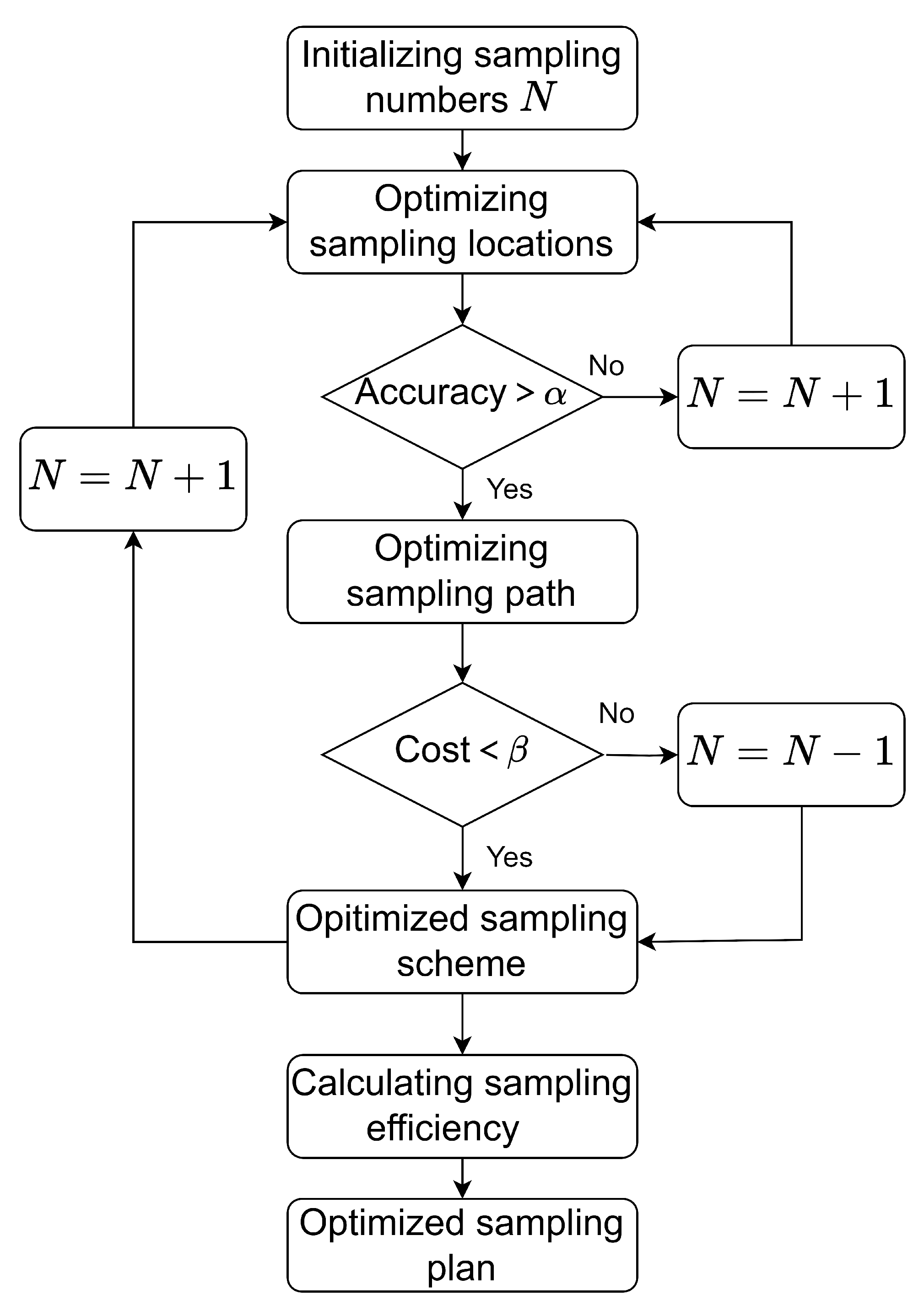
Based on the above analysis, the SSO model was developed. The overall workflow of the model is shown in Figure 2. First, for a given number of sampling points N, the spatial locations of these points are optimized to achieve the maximum possible accuracy. This maximum accuracy value is then compared with the empirical threshold $\alpha$. If the value is lower than $\alpha$, the number of sampling points is increased, and the optimization process is repeated. When the maximum accuracy exceeds $\alpha$, the UAV flight sequence among the sampling points is optimized to minimize the total sampling cost. The minimum cost obtained from this step is compared with the empirical cost threshold $\beta$. If the minimum cost is below $\beta$, the corresponding sampling configuration is retained as a feasible alternative. Otherwise, the number of sampling points is considered to have reached its upper limit.

All feasible alternatives are then ranked according to their sampling accuracy and cost to produce an optimized set of sampling schemes. Finally, the sampling efficiency of these schemes is evaluated, and the one with the highest efficiency is selected as the optimal plan. The main parameters of the SSO model used in this study are summarized in

Table 1. Parameters of the SSO model and EGA.

Parameter	Value	Description
$\alpha$	$3.33\times {10}^2$	Threshold for acceptable sampling accuracy
$\beta$	1500	Threshold for acceptable time cost
Population size	60	Number of individuals per generation
Max generations	50	Termination condition of evolution
Mutation probability	0.50	Probability of mutation
Crossover rate	0.70	Probability of crossover
Convergence threshold	$1.00\times {10}^{-6}$	Criterion for stopping evolution
Selection method	Tournament	Strategy for selecting parents
Mutation operator	Inversion	Reverses a random gene segment
Crossover operator	PMX	Partially matched crossover (permutation encoding)
Encoding type	Permutation	Suitable for route/layout optimization

.

2.3.1. Objective Function

The core task of spatial sampling with UAVs in satellite observation areas is to use the NDVI sample data acquired by UAVs to obtain an accurate representation of the overall distribution of the NDVI in the study area. It is assumed that there are m satellite image pixels in the observation area, where each image pixel includes k UAV observation pixels; thus, the study area includes a total of $mk$ UAV pixels. For the parameters to be estimated, the NDVI obtained from UAV imagery can be used as prior knowledge to update the spatial distribution, that is, by adding relative true values [4]. The representative satellite error of UAV sampling can be expressed by the following formula [26]:

$${\sigma }^2={\displaystyle \frac{1}{k}}MSE\left[1+{\displaystyle \frac{1}{n}}+{\displaystyle \frac{S_X^2+{\left(\overline{X}-\overline{x}\right)}^2}{n{s}_x^2}}\right]$$

(1)

$$MSE={\displaystyle \frac{1}{n}}\sum _{i=1}^n{\left(y_i-{\widehat{y}}_i\right)}^2$$

(2)

where MSE represents the mean squared error between the satellite observations and the true values in the UAV sampling area. $\overline{x}$ and $s_x^2$ represent the mean and variance of the sampled UAV pixels, respectively. $\overline{X}$ and $S_X^2$ represent the mean and variance of the population distribution in the study area, respectively, and n represents the number of UAV pixels sampled.

Formula (1) shows that the errors that affect sampling include the number n of sampling points, the degree to which UAV sampling represents the population distribution ${\left(\overline{X}-\overline{x}\right)}^2$, and the standard deviation of the UAV sampling pixels $s_x$. In addition, to minimize the UAV sampling error, the following optimization conditions need to be satisfied: the distribution of UAV sampling points needs to be as close to the population distribution as possible, that is, $\overline{X}-\overline{x}\to 0$; the variance between the UAV sampling points should be as large as possible, that is, $s_x\to max$; and the UAV sampling points should be distributed as widely as possible in geographic space.

In Formula (1), the number of UAV observation pixels in each satellite image is a constant value k. In the process of optimizing the sampling error, because the true value of the data in the area cannot be obtained in advance, only the satellite remote sensing data are used as prior knowledge for sampling optimization, with all data weighted equally. Therefore, the MSE is also regarded as a constant. In the process of using the algorithm for error optimization, the following formula, which is used to assess the optimization result, is used as the objective function for error optimization: $Obj=\frac{1}{n}+\frac{S_X^2+{\left(\overline{X}-\overline{x}\right)}^2}{n{s}_x^2}$.

2.3.2. Constraints

This study explores how to minimize survey error under a given cost constraint. Compared with the cost function used in conventional sampling, the cost function applied in spatial surveys is also affected by the distribution of sampling points, as well as the sample size. The impact of the sampling point distribution on cost is mainly reflected in the density of the sample distribution. With other factors unchanged, the looser the sample distribution in space is, the greater the traffic cost incurred when transferring between sampling points. We used sampling time to characterize the cost of the sampling survey, and the sampling time could be calculated with the following formula:

$$T=N·{\overline{t}}_N+{\displaystyle \frac{\mathit{min}\left({\displaystyle \sum _{i=1}^N}{d}_i\right)}{v}}$$

(3)

The total time required to complete the UAV sampling task T is composed of two factors: the total time spent on data sampling at the sampling point and the flight time between the sampling points. ${\overline{t}}_N$ is the average time spent on UAV data sampling at a single sampling point, and N is the number of sampling points for the UAV. $d_i$ is the flight speed of the UAV between the sampling points, v is the flight distance of the UAV from sampling point i to sampling point $i+1$, and $\mathit{min}\left({\displaystyle \sum _{i=1}^N}{d}_i\right)$ is the shortest path among all the UAV sampling points.

When conducting spatial sampling surveys, surveyors usually move to the nearest sampling point to continue data collection after completing data collection at each sampling point. The transportation cost can be estimated by measuring the distance between each sampling point. It is simple to implement and works well when there are few sampling points. However, as the number of sampling points increases, the distance between subsequent sampling points may increase sharply. The final total distance may be very long due to the lack of global route planning. In this study, the UAV needs to traverse all the sampling points, so the sum of the distances for all the sampling tasks must be minimized. Based on the previous analysis, the problem of calculating the distance between sampling points can be abstracted as a TSP, which is solved using an intelligent algorithm.

2.3.3. Solution Assessment

We used sampling efficiency to assess each sampling plan, that is, the sampling accuracy that could be obtained per unit cost of input. The formula for calculating the sampling efficiency is as follows:

$$E={\displaystyle \frac{\frac{1}{{\sigma }^2}}{T}}={\displaystyle \frac{1}{T{\sigma }^2}}$$

(4)

where ${\sigma }^2$ is the sampling error, $\frac{1}{{\sigma }^2}$ characterizes the sampling accuracy, and T is the time required for sampling.

2.4. Solution Algorithm

GA is a stochastic optimization method that simulates natural evolution [27]. The evolution of biological populations depends on the crossover and mutation of chromosomes. Similarly, in the GA, genetic operators act on the population $P\left(t\right)$ to perform selection, crossover, and mutation operations, thereby generating a new population $P\left(t+1\right)$ and gradually improving the fitness of solutions.

The key components of the GA are the following three operators:

Selection: Sampling locations with smaller sampling errors are preferentially selected from the previous generation and retained in the next generation.

Crossover: Pairs of sampling locations are randomly matched, and portions of their coordinate values are exchanged with a certain probability (the crossover rate).

Mutation: Some coordinate values within the sampling locations are replaced by those of other locations with a given mutation probability, enhancing population diversity.

To avoid premature convergence and preserve optimal solutions, the elitist retention strategy [28] is adopted. In this approach, the best individuals (elite solutions) found during evolution are directly carried over to the next generation without crossover or mutation. This modification significantly enhances the global convergence capability of the standard GA.

Therefore, the elitist genetic algorithm (EGA), incorporating the elitist retention mechanism, was applied in this study to solve the SSO model. During the optimization process, the sampling configuration with the minimum sampling error is preserved for the next iteration to ensure convergence toward the global optimum. The main parameters of the EGA used in this study are summarized in Table 1.

3. Materials and Methods

3.1. Study Area

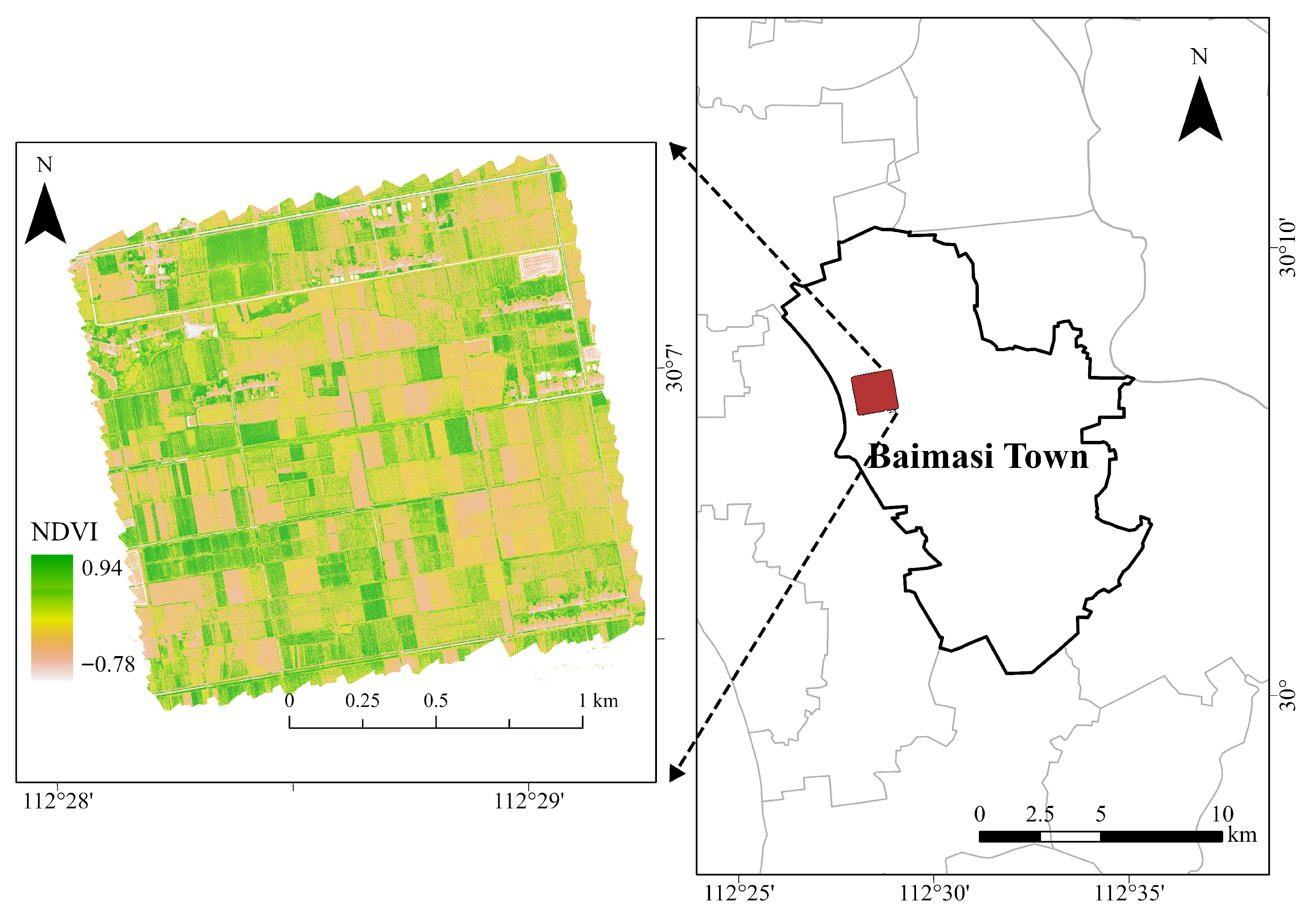
The experiment was conducted in a rapeseed field located in Baimasi Town, Jiangling County, Hubei Province, China (Figure 3). The study area covers approximately 2.5 ha of farmland characterized by flat terrain with gentle slopes and an elevation of 26.1–31.2 m. The soil type is predominantly paddy soil with relatively uniform physical properties. At the time of sampling, rapeseed was planted across all fields, exhibiting uniform growth conditions. The mean NDVI for the entire farmland was 0.40, with a standard deviation of 0.22.

Baimasi Town has an average annual temperature of 16.6 °C and a mean annual precipitation of approximately 1045 mm. The main crops cultivated in this region include rice, wheat, rapeseed, and cotton. Benefiting from sufficient water and thermal resources, the area represents a typical farmland ecosystem of the Jianghan Plain. The site was intentionally selected for its relatively homogeneous topography and soil conditions, which minimize external variability and provide a suitable environment for evaluating the effectiveness of the proposed SSO model in optimizing spatial sampling design.

3.2. Satellite Image Data

The Sentinel-2 satellite, composed of two high-resolution satellites (2A and 2B), has a revisit period of 5 days. In this study, the Sentinel-2 satellite image data provided was downloaded by Google Earth Engine at nearby time points in the study area for processing. To avoid cloud pollution, images with less than 30% cloud coverage were selected (8 November 2021). Each image was processed by cloud masking and median synthesis to generate a resulting high-quality cloud-free image. The 10-m NDVI image was calculated based on the B4 band (band centered at 665 nm) and B8 band (band centered at 842 nm) of Sentinel-2 and was used as the initial information for optimization. The Level-2A product, which provides surface reflectance corrected for atmospheric effects, was used to ensure radiometric consistency with the UAV data.

3.3. UAV Image Data

UAV-based remote sensing mapping was performed in a large-scale field with uniform rapeseed growth in Baimasi town, Jiangling County, Hubei Province, on 11 November 2021. A Phantom 4 UAV (DJI Innovations, Shenzhen, China) was used for data collection under clear and calm weather conditions from 10:00 to 14:00 (local time, UTC + 8), with the heading overlap rate of 85.0%, and the side overlap rate of 70.0%. The imagery, with a ground resolution of approximately 6 cm/pixel, was radiometrically calibrated to surface reflectance using an on-site reflectance panel to ensure compatibility with the satellite data. The orthorectified UAV images were co-registered to the Sentinel-2 NDVI image and resampled to 10 m resolution using bilinear interpolation for pixel-level correspondence. NDVI was then calculated from the red (650 nm) and near-infrared (840 nm) bands to obtain relative ground-truth values for validation.

3.4. Assessment of the SSO Model

To demonstrate and validate the effect of the SSO model proposed in this paper, different sampling plans were implemented for a representative area, and the accuracy of data acquisition and the sampling cost of the different plans were compared and assessed.

Conventional spatial sampling methods are based on probability sampling and include simple random sampling (samples are selected entirely at random without any prior grouping of the population), systematic sampling (samples are selected at fixed intervals determined by the required sample size), and stratified sampling (samples are randomly selected from different strata of the population according to specified proportions).

One experimental group and four control groups were created to validate the performance of the model. For the experimental group, the SSO-optimized sampling plan was used. For the control group, the existing conventional sampling plans, namely, simple random sampling, systematic sampling, and stratified sampling with an equal distribution and a Neyman distribution, were used. The sampling cost and sampling accuracy of the experimental group were compared with those of the control group to verify the feasibility of the SSO-optimized plan.

For the simple random sampling control group, a certain number of coordinates were randomly selected from the set of candidate coordinates that met the accuracy requirements to determine the locations of the UAV sampling points, and the sampling accuracy and the cost required for the UAV to complete the flight sampling were calculated.

For the systematic sampling group, a certain number of coordinates were selected at equal intervals from the set of candidate coordinates that met the accuracy requirements, and the remaining steps were the same as those in simple random sampling. The spacing of systematic sampling was determined based on the size of the candidate coordinate set and the number of sampling points.

In this study, according to the number of sampling points in each stratum, stratified sampling was subdivided into stratified sampling with an equal distribution and stratified sampling with a Neyman distribution, yielding two different control groups. For an equal distribution, the number of sampling points selected in each stratum is the same; the Neyman distribution is the optimal distribution for sample units when the cost coefficient of each stratum is the same. Suppose $n_h$ is the sample content of each stratum, n is the total sample size, $S_h$ is the standard deviation of samples from stratum h, $W_h$ is the weight of each stratum, $N_h$ is the total number of units in stratum h, L is the total number of strata, and under the Neyman distribution, the sample size is proportional to the stratum weight ($W_h$) multiplying the strata standard deviation ($S_h$); thus, the sample size for each stratum can be calculated by the following formula:

$$n_h=n{\displaystyle \frac{W_h{S}_h}{{\displaystyle \sum _{h=1}^L}{W}_h{S}_h}}=n{\displaystyle \frac{N_h{S}_h}{{\displaystyle \sum _{h=1}^L}{N}_h{S}_h}}$$

(5)

After successfully determining whether a coordinate could be a candidate coordinate, the mean value of the NDVI at the selected coordinate point in the upper-left corner of the sampling frame was calculated, and the candidate coordinates were divided into 6 strata according to the NDVI value and labeled. In stratified sampling, different labels represent different strata, and random sampling is performed for each stratum. Considering that the sample size may vary among strata, the roulette wheel selection algorithm was introduced to select among the strata, and the probability of being selected was proportional to the value of the corresponding fitness function $f\left(x_h\right)$. For the stratum in which each sample unit was located, the probability of being selected was:

$$P\left(x_i\right)={\displaystyle \frac{f\left(x_i\right)}{{\displaystyle \sum _{h=1}^L}f\left(x_h\right)}}$$

(6)

$$f\left(x_h\right)={\displaystyle \frac{n_h}{n}}$$

(7)

Subsequently, the cumulative probability of each stratum was calculated and used to represent the sum of the selection probabilities of all the strata. This was equivalent to the ߢspan’ of samples, and the larger the ߢspan’ was, the more likely a sample point in a given stratum was of being selected.

Finally, a randomization function was used to randomly generate numbers between 0 and 1, and the results were compared to those obtained based on a cumulative probability distribution. Sampling was performed in the stratum with which the randomly generated number was associated. To reduce the stochasticity of sampling and algorithms, each sampling method was implemented 20 times to compare the average sampling efficiency.

4. Results

In this study, we proposed an SSO model for optimizing the layout and configuration of satellites and UAVs in a satellite–UAV integrated remote sensing agricultural monitoring system. This model aims to fully harness the potential of integration between satellites and UAVs.

The SSO model was applied to the field survey data in the study area. It produced 16 optimized sampling plans that met the required accuracy levels for sampling. These plans varied in sampling point numbers and locations. Next, we compared the SSO-optimized sampling scheme with the conventional sampling schemes used in four control groups.

4.1. Sampling Optimization

Figure 4, Figure 5, Figure 6, Figure 7 and Figure 8 show the results of spatial sampling optimization of the satellite–UAV integrated remote sensing agricultural monitoring system.

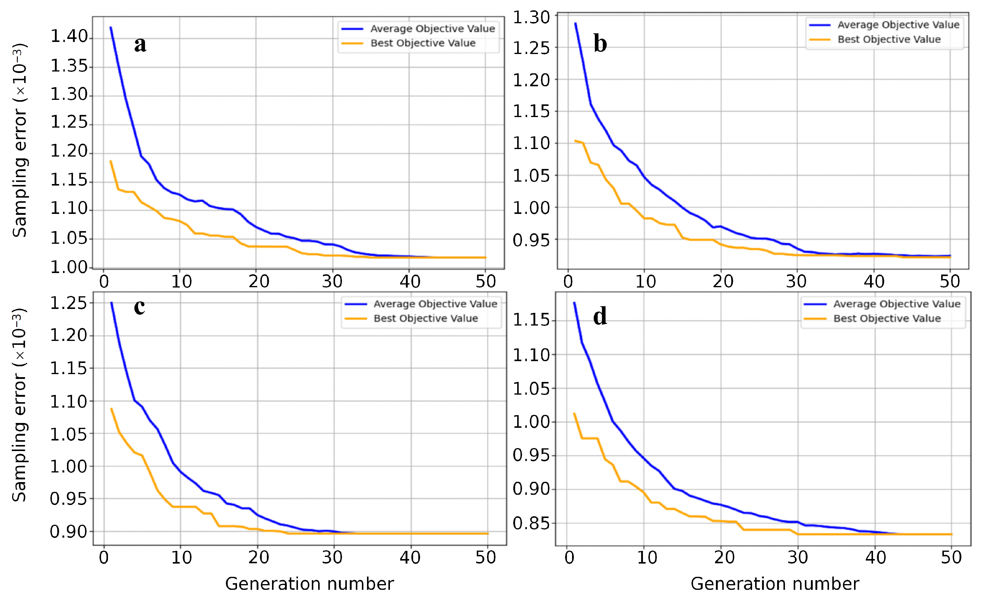
The subplots labeled a, b, c, and d in Figure 4 display the optimization curves for the minimum sampling error. These curves represent the results obtained when we have 13, 14, 15, and 16 sampling points, respectively. It is evident that the error values consistently decrease as the EGA progresses through 50 generations, ultimately reaching the minimum values. The average sampling error value of the population was reduced by more than 27.3%. The error value for the best individual in the population was reduced by about 16.1%.

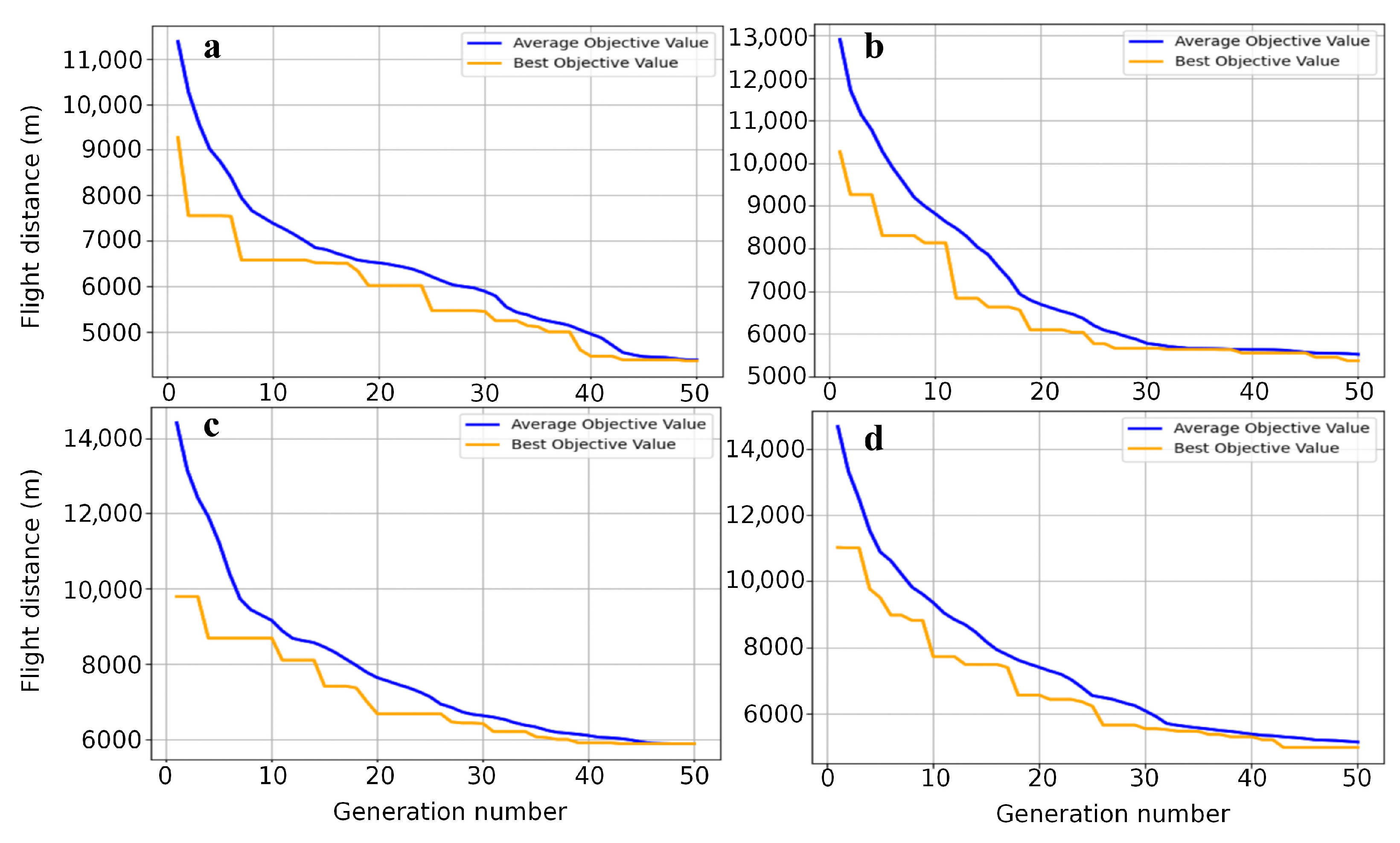
The subplots labeled a, b, c, and d in Figure 5 show the optimization curves for the total distance traveled when we have 13, 14, 15, and 16 sampling points, respectively. The distance the UAV flies depends on the order in which it visits the sampling points. The UAV’s flight distance is continuously improved and reduced using EGA. The average sampling distance can be reduced by 7000 to 8000 m through EGA optimization. Most of the final distances fall between 5000 m and 6000 m, less than half of the non-optimized paths. The EGA is highly effective in solving this problem.

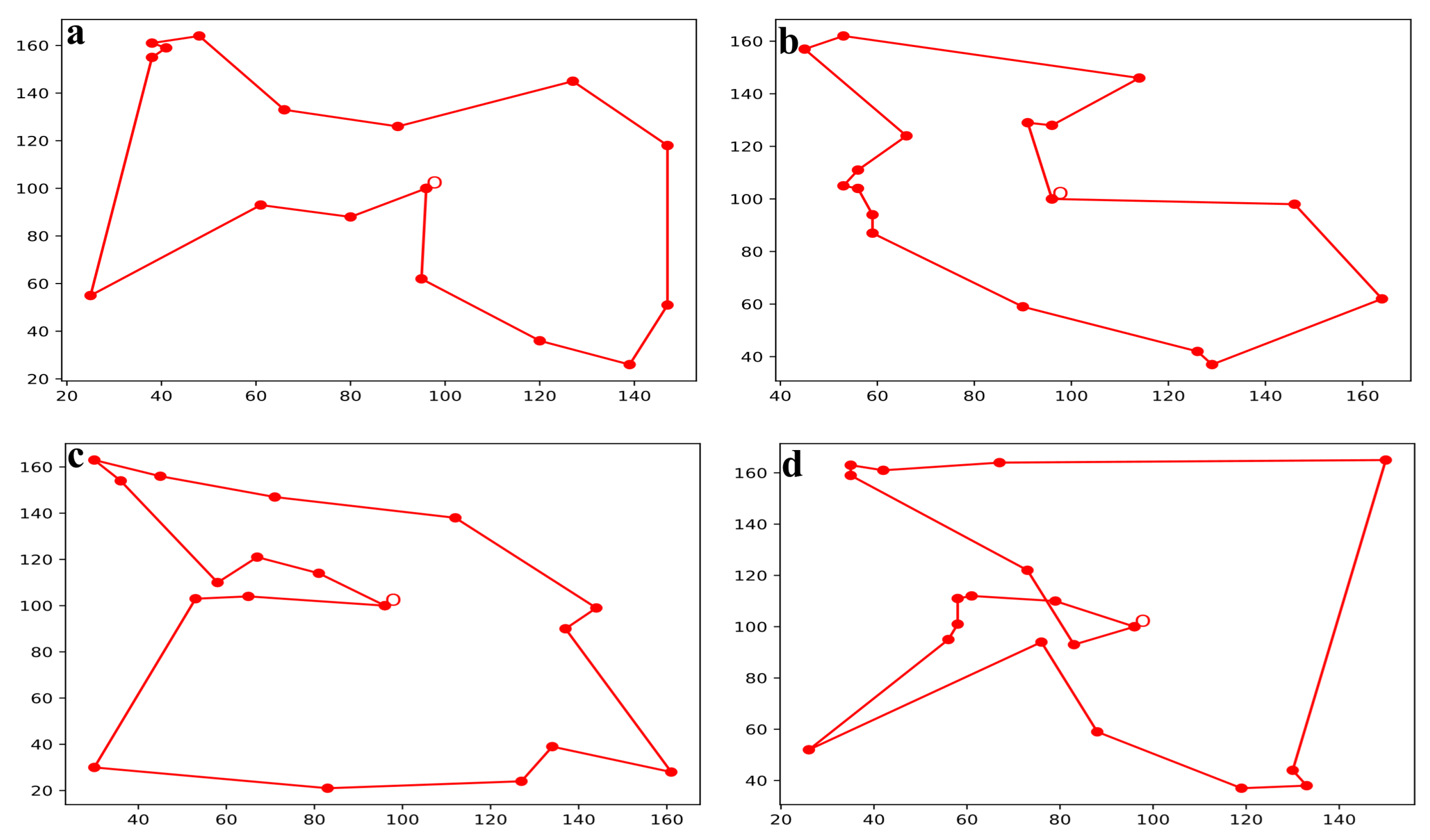
The subplots labeled a, b, c, and d in Figure 6 show the flight paths of the UAVs in the study area when the number of sampling points is 13, 14, 15, and 16, respectively, where point O is the center of the study area, which also serves as the takeoff point and recovery point of the UAV. The sampling points of the UAV sampling survey in the figure are more evenly distributed in the figure, and the sampling points in the northern region are slightly denser, which is relatively in line with the actual cultivation situation in the study area. The crops grown in the study area are relatively homogeneous and uniform, and more sampling points are needed to accurately monitor the growth of crops in the more variable parts of the study area.

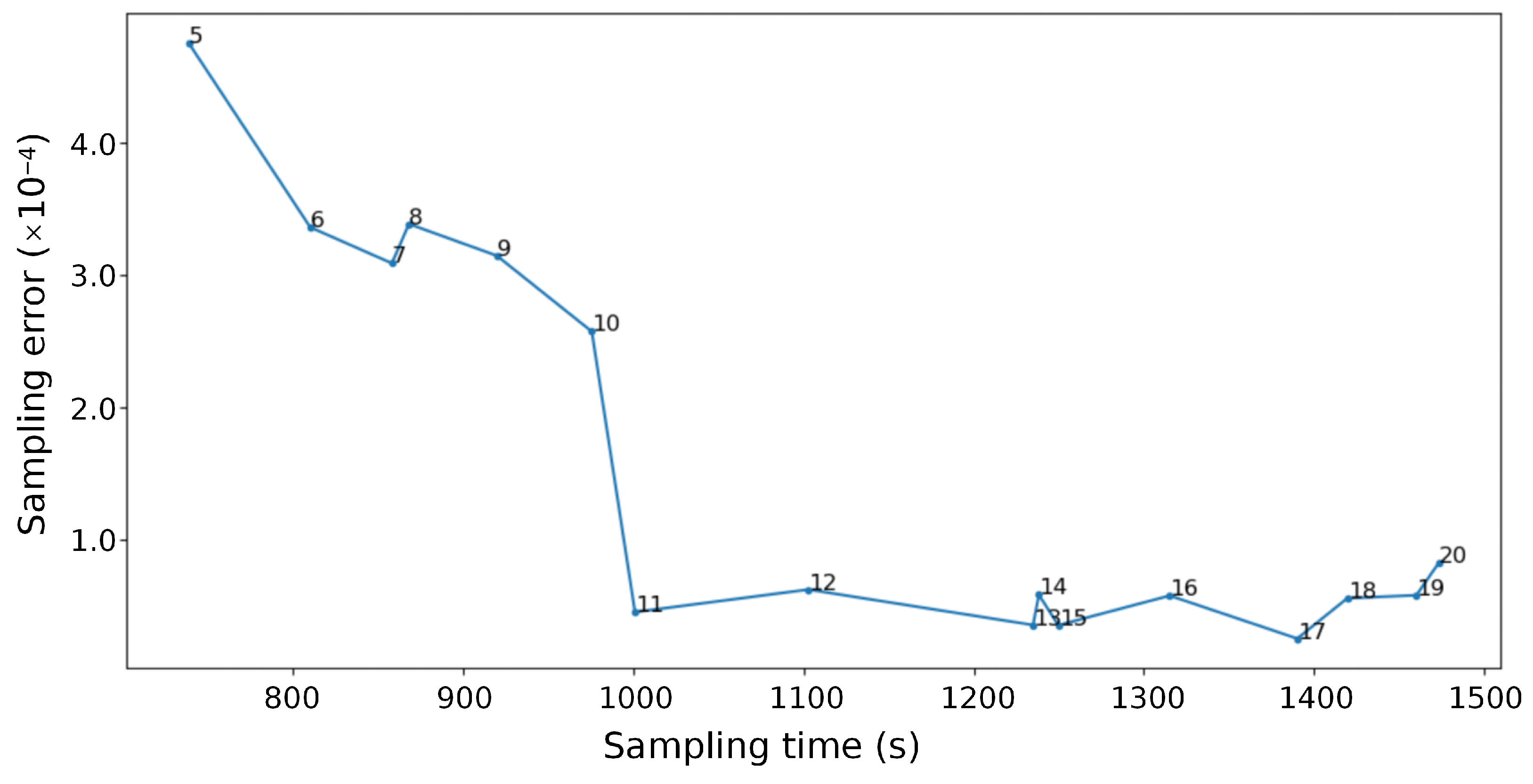
Figure 7 shows the cost-accuracy curve based on the set of sampling plans, where the horizontal coordinate is the total time taken to complete the sampling task, the vertical coordinate is the error used to sample the satellite data with UAV low-altitude remote sensing, and the dot label is the number of sampling points. There are 16 sampling plans in the sampling plans set for different numbers of sampling points. As the number of sampling points increases, the total time to complete the sampling task increases. It takes 739 s to complete the sampling of 5 points, and it takes the most time to sample 20 sampling points, which is 1473 s. With the increase in the number of sampling points, the sampling error shows a decreasing trend as a whole, and the lowest error value is that of setting up 17 sampling points, with an error value of $2.52\times {10}^{-5}$.

Overall, the sampling plans with more sampling points consumed more time and cost, but had less sampling error. It is in line with the general principle of sampling, i.e., the accuracy of the estimation can be obtained by increasing costs or the number of samples. The SSO model can obtain considerable accuracy improvement by increasing the cost.

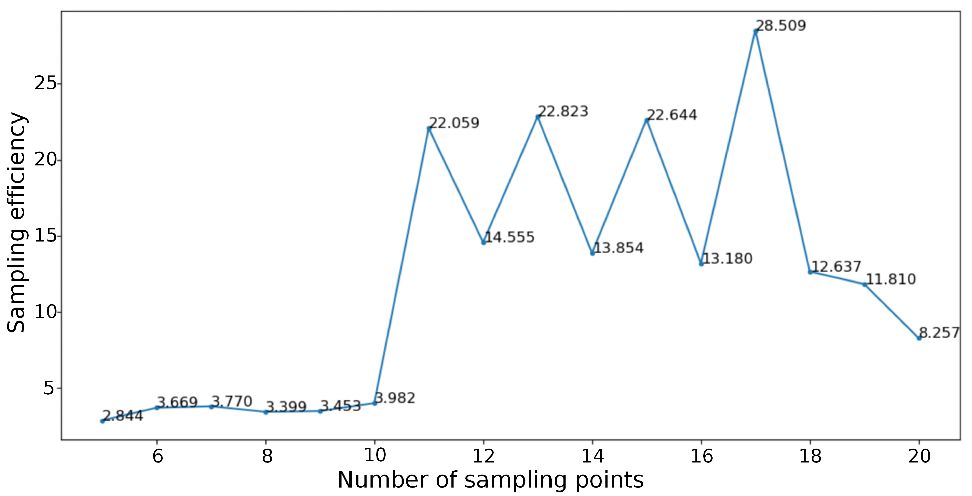
The sampling efficiency of each sampling plan is calculated using Formula (4). We plot the sampling efficiency curve for each sampling plan in the study area, as shown in Figure 8. Among these plans, using 11 to 17 sampling points yields higher efficiency, and the peaks occur at 11, 13, and 15 sampling points, all exceeding 22. The plan with 17 sampling points has the highest efficiency at 28.509. Subsequently, the efficiency decreases. Therefore, the plan with 17 sampling points is the final optimized result.

4.2. Comparison of Sampling Methods

4.2.1. Maximum Number of Sampling Points

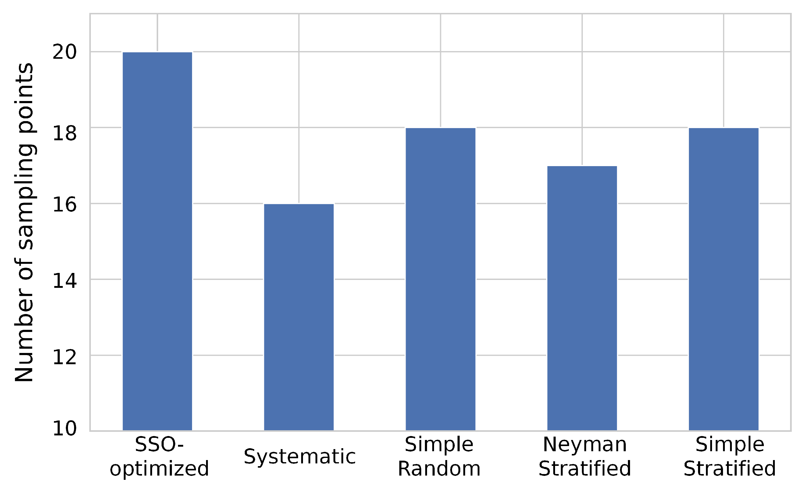
The maximum number of sampling points that can be provided by different sampling methods under the cost constraint was shown in Figure 9. In complex schemes with multiple sampling points, the conventional sampling schemes can no longer meet the predefined cost constraints and can only give 16 to 18 sampling points. The SSO model, on the other hand, is able to minimize costs through planning, resulting in 20 sampling points. This is at least 11.1% more than the number of sampling points given by the conventional sampling schemes.

4.2.2. Cost and Accuracy

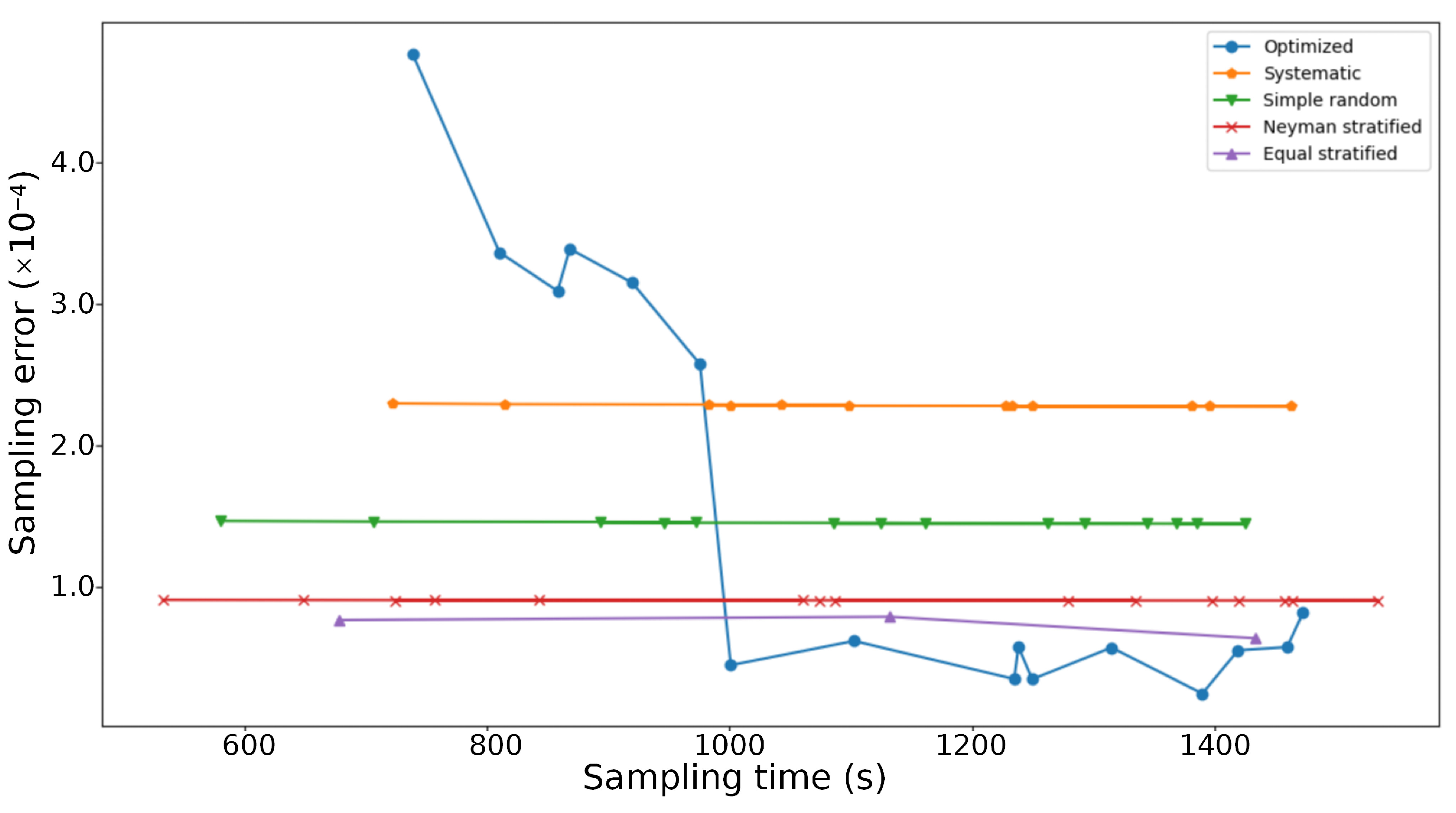
Figure 10 shows the cost and accuracy of the SSO-optimized sampling scheme and the conventional sampling schemes. Among the 12 systematic sampling plans that fulfill the cost and accuracy requirements, the sampling error remains at approximately $2.28\times {10}^{-4}$ and does not manifestly change as the number of sampling points increases. A total of 14 plans meet the cost and accuracy requirements for simple random sampling, with a sampling error maintained at around $1.45\times {10}^{-4}$, which is consistently lower than the error of systematic sampling. For stratified sampling with Neyman’s allocation, 13 plans meet the cost and accuracy requirements. The sampling error is significantly lower than systematic and simple random sampling, with an average of $9.10\times {10}^{-5}$ and slight fluctuations. However, since the number of sampling points selected for the equal stratified sampling must be a multiple of the number of strata, only three plans meet the requirements. These three plans have lower overall error levels than the remaining three conventional sampling plans, ranging from a minimum of $6.42\times {10}^{-5}$ with 18 sampling points to a maximum of $7.94\times {10}^{-5}$ with 12 sampling points.

The initial six SSO-optimized plans have higher error values and less obvious optimization effects. Starting from the 11th sampling point, the sampling error is lower than all the conventional sampling plans, and the complex situation of multiple sampling points can effectively compress the cost and provide more alternatives, so the SSO-optimized sampling scheme has a better optimization effect in the plan of the number of sampling points is higher.

Figure 11 demonstrates the difference in sampling efficiency between the SSO-optimized sampling scheme and the conventional sampling schemes. The efficiency of systematic sampling is relatively low, with an average of 4.03, and does not improve significantly when the number of sampling points increases. The efficiency of simple random sampling fluctuates slightly, with a low overall level, the highest being 11.73 at five sampling points. The efficiency of Neyman stratified sampling fluctuates manifestly but is always higher than that of simple random sampling and systematic sampling, with the highest being 20.56 at five sampling points, while there is a wave at 10 and 14 sampling points. Equal stratified sampling has the highest efficiency at six sampling points, followed by a decrease. The efficiency of the SSO-optimized sampling scheme is higher than conventional sampling schemes in all plans with more than 11 sampling points, with the highest efficiency of 28.51 at 17 sampling points. The highest efficiency among the conventional sampling plans was achieved by Neyman stratified sampling with 5 sampling points, yielding an efficiency of 20.56. In contrast, the SSO-optimized plan included 17 sampling points and achieved an efficiency of 28.51, corresponding to a 38.7% improvement over the best-performing conventional scheme. Moreover, when the number of sampling points exceeded 11, all conventional sampling methods performed worse than the SSO-optimized plan.

To quantify the variability across the 20 repeated runs, we calculated the standard deviation of sampling efficiency for each sampling method and each sampling size. Across all methods, the standard deviations were generally small (coefficient of variation less than 5%), indicating limited algorithmic stochasticity relative to the performance gaps among methods.

4.2.3. SSO-Optimized Plan

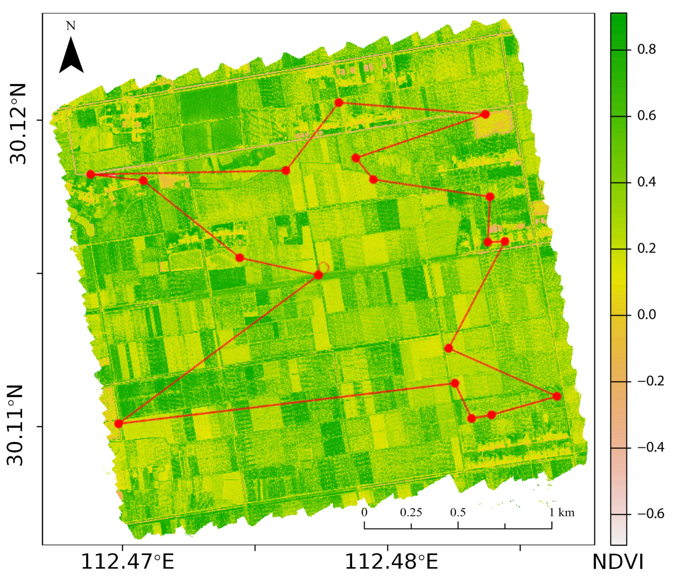
Figure 12 shows the distribution of the 17 sampling points in the SSO-optimized plan within the study area.

In the SSO-optimized sampling scheme, 11 sampling points were located in the northern part of the study area, and 6 points were located in the southern part of the study area, in addition to the UAV recovery point O. The sampling points are more densely distributed in the northern region of the study area, which is in line with the characteristics of crop growth changes in the study area, i.e., the northern growth condition fluctuates more.

5. Discussion

5.1. The Unique Value of EGA in Solving SSO Model

EGA is one of the representative heuristic algorithms [29] that centers on finding the optimal solution in the search space through genetic operations such as selection, crossover, and mutation. Our results showed that EGA can solve the SSO model smoothly. Even in the case of different sampling points, EGA can reduce the sampling error and sampling distance very well. This study confirmed the stability of EGA in efficiently solving the sampling task across various sampling points within the designated study area. Moreover, our study found that EGA does not need to be driven by massive amounts of labeled data [30]. It focuses on the objective function of the optimization problem rather than relying on data for learning. Even with limited data, GAs can search for optimal solutions through evolutionary operations. Compared to machine learning methods, it can not only achieve parallelization acceleration through independent individual fitness evaluation. Besides, EGA does not require any a priori modeling assumptions [31]. It directly evaluates the merits of the solution through a fitness function, which allows it to be easily transferred to solving other problems [27]. These advantages make the SSO model a universally applicable method that can be directly applied to spatial sampling design in different study areas.

5.2. SSO Model Improved the Sampling Efficiency

The SSO model achieved better performance than conventional sampling schemes (simple random sampling, systematic sampling, equal stratified sampling, and Neyman stratified sampling), largely due to the spatial heterogeneity inherent in agroecosystems. Crop growth rarely follows uniform spatial patterns because it is influenced by multiple factors at the field scale, such as soil conditions, crop genotype, and agricultural management. By incorporating prior spatial information and explicitly optimizing sampling locations, the SSO model is better able to capture this heterogeneity than simple random or systematic sampling. Consequently, in areas with strong spatial variability, the SSO-optimized sampling plan naturally allocates more sampling points to regions with larger NDVI variation. This spatial adaptiveness distinguishes the SSO approach from conventional schemes [10]. Compared with equal and Neyman stratified sampling, the SSO model can further improve sampling efficiency under the same cost constraints by optimizing both the placement of sampling points and the UAV flight path. In addition, conventional schemes showed only marginal accuracy improvements when sampling cost increased in our study area, likely due to the cost constraints and the monoculture setting.

The superior performance of the SSO model can also be explained by the spatial structure of NDVI in agricultural fields. NDVI typically exhibits clear spatial autocorrelation, reflecting gradual changes caused by underlying biophysical processes. By jointly optimizing the number and spatial configuration of UAV sampling points, the SSO model captures these structured spatial patterns more effectively and reduces uncertainty in NDVI estimation. The SSO-optimized sampling plan enhances the representativeness of UAV observations and strengthens the complementarity between satellite and UAV-based remote sensing. This mechanistic foundation explains why the SSO model consistently achieves higher sampling efficiency and estimation accuracy within the satellite–UAV integrated remote sensing framework.

5.3. Limitations and Future Directions

In solving the optimization problem of spatial sampling, the SSO model was capable of generating sampling schemes with different numbers of sampling points that satisfied the accuracy and cost requirements. However, the efficiency of the SSO-optimized sampling scheme is lower than conventional sampling schemes when the number of sampling points is small (≤10). This is mainly because the search space becomes highly discrete under small-sample configurations, which limits the potential for layout optimization and increases the sensitivity of GAs to initial population settings. As a result, the algorithm may more easily become trapped in local optima [32]. To mitigate this issue, users may adjust the algorithm settings, such as increasing population diversity, using multi-start initialization, or employing hybrid optimization strategies, depending on the scale of the problem.

Additionally, although we have successfully optimized UAV sampling in rapeseed fields, the generalizability of the proposed SSO model to different crops and heterogeneous agricultural systems remains to be further validated. In the future, additional practical factors, such as the number of UAVs, battery replacements, and instrument depreciation rate are likely necessary to provide a more comprehensive measurement of the sampling cost. Moreover, the same optimization logic can be extended to integrate ground-based measurements by incorporating ground sampling efficiency as an additional cost layer. This extension will contribute to developing space–air–ground integrated networks in future research.

6. Conclusions

In this paper, we conceptualized the configuration of the satellite–UAV integrated agricultural monitoring system as a spatial sampling problem and proposed an SSO model to optimize UAV sampling within the satellite monitoring coverage, thereby improving the efficiency of satellite–UAV integration. In the study, we found the following:

• The SSO model can improve the efficiency of observations by optimizing the sampling design. Under the same cost constraint, the SSO model increased the number of sampling points by at least 11.1% and the sampling efficiency was at least 38.7% higher than the conventional sampling plans.
• The heuristic algorithm helps to solve the multi-objective optimization problem. The EGA can efficiently solve the SSO model optimally. The average sampling error of the final SSO-optimized plan was reduced by about 27.3%, and the sampling distance was shortened by 7000 to 8000 m.
• The problem of optimizing the layout of satellite remote sensing and UAV-based remote sensing can be transformed into a spatial sampling problem. It is necessary to consider cost constraints and increase efficiency by applying optimization methods in agricultural monitoring and government census in the future.

References

1. Ghamisi, P.; Rasti, B.; Yokoya, N.; Wang, Q.; Hofle, B.; Bruzzone, L.; Bovolo, F.; Chi, M.; Anders, K.; Gloaguen, R.; et al. Multisource and Multitemporal Data Fusion in Remote Sensing: A Comprehensive Review of the State of the Art. IEEE Geosci. Remote Sens. Mag. 2019, 7, 6–39. [Google Scholar] [CrossRef]
2. Zhao, Z.; Wang, F.; Xiao, Y.; Liu, L.; Chen, N.; Weng, W.; Peng, D.; Zhang, X.; Shi, Z. Development and Evaluation of Remote Sensing-Derived Relative Growth Rate (RGR) for Rice Yield Estimation. IEEE J. Sel. Top. Appl. Earth Obs. Remote Sens. 2025, 18, 25735–25747. [Google Scholar] [CrossRef]
3. Alvarez-Vanhard, E.; Corpetti, T.; Houet, T. UAV & Satellite Synergies for Optical Remote Sensing Applications: A Literature Review. Sci. Remote Sens. 2021, 3, 100019. [Google Scholar] [CrossRef]
4. Kattenborn, T.; Lopatin, J.; Förster, M.; Braun, A.C.; Fassnacht, F.E. UAV Data as Alternative to Field Sampling to Map Woody Invasive Species Based on Combined Sentinel-1 and Sentinel-2 Data. Remote Sens. Environ. 2019, 227, 61–73. [Google Scholar] [CrossRef]
5. Bhardwaj, A.; Sam, L.; Akanksha; Martín-Torres, F.J.; Kumar, R. UAVs as Remote Sensing Platform in Glaciology: Present Applications and Future Prospects. Remote Sens. Environ. 2016, 175, 196–204. [Google Scholar] [CrossRef]
6. Alvarez-Vanhard, E.; Houet, T.; Mony, C.; Lecoq, L.; Corpetti, T. Can UAVs Fill the Gap Between In Situ Surveys and Satellites for Habitat Mapping? Remote Sens. Environ. 2020, 243, 111780. [Google Scholar] [CrossRef]
7. Gevaert, C.M.; Suomalainen, J.; Tang, J.; Kooistra, L. Generation of Spectral–Temporal Response Surfaces by Combining Multispectral Satellite and Hyperspectral UAV Imagery for Precision Agriculture Applications. IEEE J. Sel. Top. Appl. Earth Obs. Remote Sens. 2015, 8, 3140–3146. [Google Scholar] [CrossRef]
8. Bazrafkan, A.; Igathinathane, C.; Bandillo, N.; Flores, P. Optimizing Integration Techniques for UAS and Satellite Image Data in Precision Agriculture—A Review. Front. Remote Sens. 2025, 6, 1622884. [Google Scholar] [CrossRef]
9. Kuenzer, C.; Dech, S.; Wagner, W. Remote Sensing Time Series Revealing Land Surface Dynamics: Status Quo and the Pathway Ahead. In Remote Sensing Time Series: Revealing Land Surface Dynamics; Kuenzer, C., Dech, S., Wagner, W., Eds.; Remote Sensing and Digital Image Processing; Springer International Publishing: Cham, Switzerland, 2015; pp. 1–24. [Google Scholar] [CrossRef]
10. Wang, J.F.; Stein, A.; Gao, B.B.; Ge, Y. A Review of Spatial Sampling. Spatial Stat. 2012, 2, 1–14. [Google Scholar] [CrossRef]
11. Stevens, D.L., Jr.; Olsen, A.R. Spatially Balanced Sampling of Natural Resources. J. Am. Stat. Assoc. 2004, 99, 262–278. [Google Scholar] [CrossRef]
12. Xiao, Y.; Zhao, Z.; Huang, J.; Huang, R.; Weng, W.; Liang, G.; Zhou, C.; Shao, Q.; Tian, Q. The Illusion of Success: Test Set Disproportion Causes Inflated Accuracy in Remote Sensing Mapping Research. Int. J. Appl. Earth Obs. Geoinf. 2024, 135, 104256. [Google Scholar] [CrossRef]
13. Dunn, R.; Harrison, A.R. Two-Dimensional Systematic Sampling of Land Use. J. R. Stat. Soc. C (Appl. Stat.) 1993, 42, 585–601. [Google Scholar] [CrossRef]
14. Lu, Y.; Xie, H.; Zhang, J.; Jin, Y.; Feng, Y.; Gong, Y.; Han, W.; Zhang, H.; Tong, X. Fractal Theory Based Stratified Sampling for Quality Assessment of Remote-Sensing-Derived Geospatial Data. IEEE J. Sel. Top. Appl. Earth Obs. Remote Sens. 2023, 16, 7100–7111. [Google Scholar] [CrossRef]
15. Wang, J.F.; Christakos, G.; Hu, M.G. Modeling Spatial Means of Surfaces with Stratified Nonhomogeneity. IEEE Trans. Geosci. Remote Sens. 2009, 47, 4167–4174. [Google Scholar] [CrossRef]
16. Yang, M.; Chen, S.; Xu, D.; Hong, Y.; Li, S.; Peng, J.; Ji, W.; Guo, X.; Zhao, X.; Shi, Z. Strategies for Predicting Soil Organic Matter in the Field Using the Chinese Vis-NIR Soil Spectral Library. Geoderma 2023, 433, 116461. [Google Scholar] [CrossRef]
17. Lu, R.; Liao, R.; Meng, R.; Hu, Y.; Zhao, Y.; Guo, Y.; Zhang, Y.; Shi, Z.; Ye, S. Strategic Sampling for Training a Semantic Segmentation Model in Operational Mapping: Case Studies on Cropland Parcel Extraction. Remote Sens. Environ. 2025, 331, 115034. [Google Scholar] [CrossRef]
18. Zhang, Z.; Zhu, L. A Review on Unmanned Aerial Vehicle Remote Sensing: Platforms, Sensors, Data Processing Methods, and Applications. Drones 2023, 7, 398. [Google Scholar] [CrossRef]
19. Wang, L.; Zhang, X.; Qin, K.; Wang, Z.; Zhou, J.; Song, D. AoI Analysis of Satellite–UAV Synergy Real-Time Remote Sensing System. Remote Sens. 2024, 16, 3305. [Google Scholar] [CrossRef]
20. Zhao, H.; Ji, F.; Wang, Y.; Yao, K.; Chen, F. Space–Air–Ground–Sea Integrated Network with Federated Learning. Remote Sens. 2024, 16, 1640. [Google Scholar] [CrossRef]
21. Haining, R. Spatial Data Analysis: Theory and Practice; Cambridge University Press: Cambridge, UK, 2003. [Google Scholar] [CrossRef]
22. GB/T 39612-2020; Specifications for Low-Altitude Digital Aerial Photography and Data Processing. Ministry of Natural Resources, People’s Republic of China: Beijing, China, 2020.
23. Lyu, Y.; Wang, S.; Hu, T.; Pan, Q. UAV Coverage Path Planning of Multiple Disconnected Regions Based on Cooperative Optimization Algorithms. IEEE Trans. Cogn. Dev. Syst. 2025, 17, 259–270. [Google Scholar] [CrossRef]
24. Alemayehu, T.S.; Kim, J.H. Efficient Nearest Neighbor Heuristic TSP Algorithms for Reducing Data Acquisition Latency of UAV Relay WSN. Wirel. Pers. Commun. 2017, 95, 3271–3285. [Google Scholar] [CrossRef]
25. Dong, R.; Wang, S.; Wang, G.; Wang, X. Hybrid Optimization Algorithm Based on Wolf Pack Search and Local Search for Solving Traveling Salesman Problem. J. Shanghai Jiaotong Univ. (Sci.) 2019, 24, 41–47. [Google Scholar] [CrossRef]
26. Zeng, Y.; Li, J.; Liu, Q.; Li, L.; Xu, B.; Yin, G.; Peng, J. A Sampling Strategy for Remotely Sensed LAI Product Validation over Heterogeneous Land Surfaces. IEEE J. Sel. Top. Appl. Earth Obs. Remote Sens. 2014, 7, 3128–3142. [Google Scholar] [CrossRef]
27. Holland, J.H. Outline for a Logical Theory of Adaptive Systems. J. ACM 1962, 9, 297–314. [Google Scholar] [CrossRef]
28. Suzuki, J. A Markov Chain Analysis on Simple Genetic Algorithms. IEEE Trans. Syst. Man Cybern. 1995, 25, 655–659. [Google Scholar] [CrossRef]
29. Ilin, V.; Simić, D.; Simić, S.D.; Simić, S.; Saulić, N.; Calvo-Rolle, J.L. A Hybrid Genetic Algorithm, List-Based Simulated Annealing Algorithm, and Different Heuristic Algorithms for the Travelling Salesman Problem. Log. J. IGPL 2023, 31, 602–617. [Google Scholar] [CrossRef]
30. Baeck, T.; Fogel, D.B.; Michalewicz, Z. (Eds.) Handbook of Evolutionary Computation; CRC Press: Boca Raton, FL, USA, 1997. [Google Scholar] [CrossRef]
31. Jordan, M.I.; Mitchell, T.M. Machine Learning: Trends, Perspectives, and Prospects. Science 2015, 349, 255–260. [Google Scholar] [CrossRef]
32. Katoch, S.; Chauhan, S.S.; Kumar, V. A Review on Genetic Algorithm: Past, Present, and Future. Multimed. Tools Appl. 2021, 80, 8091–8126. [Google Scholar] [CrossRef]
Figure 1. Satellite–UAV integrated remote sensing system for agricultural monitoring.
Remotesensing 17 03895 g001
Figure 2. Workflow of the SSO model.
Remotesensing 17 03895 g002
Figure 3. Overview map of the study area.
Remotesensing 17 03895 g003
Figure 4. Sampling error optimization curves for the study area (partial). (ad) represent cases with 13 to 17 sampling points, respectively.
Remotesensing 17 03895 g004
Figure 5. Total sampling distance optimization curves for the study area (partial). (ad) represent cases with 13 to 17 sampling points, respectively.
Remotesensing 17 03895 g005
Figure 6. UAV flight path in the study area (partial). (ad) represent cases with 13 to 17 sampling points, respectively.
Remotesensing 17 03895 g006
Figure 7. Sampling cost–accuracy curve for the study area.
Remotesensing 17 03895 g007
Figure 8. Sampling efficiency curves for each sampling plan in the study area.
Remotesensing 17 03895 g008
Figure 9. Maximum number of sampling points for each scheme.
Remotesensing 17 03895 g009
Figure 10. Comparison of cost–accuracy curves for each plan.
Remotesensing 17 03895 g010
Figure 11. Comparison of sampling efficiency curves for each plan.
Remotesensing 17 03895 g011
Figure 12. UAV flight route map for the SSO-optimized sampling plan, with red points connected by lines indicating the sampling points along the flight path.
Remotesensing 17 03895 g012