Waveform Analysis for Enhancing Airborne LiDAR Bathymetry in Turbid and Shallow Tidal Flats of the Korean West Coast

Highlights

What are the main findings?

• An adaptive progressive Gaussian decomposition (APGD) technique was proposed to enhance airborne bathymetric LiDAR (ABL) waveform processing in shallow and turbid tidal flat environments.
• The proposed approach enhanced seabed detection reliability, achieving up to 70% coverage in turbid tidal flats and enabling bathymetric mapping in areas previously unmeasurable by conventional LiDAR and MBES systems.

What are the implications of the main findings?

• The proposed APGD framework enables robust and accurate bathymetric mapping under complex conditions, supporting continuous monitoring of tidal flat geomorphology.
• The Gaussian-based APGD enables the extraction of various waveform features for each point, providing a foundation for extended applications such as water–land boundary detection and submerged object identification.

Abstract

Tidal flats play a vital role in coastal ecosystems by supporting biodiversity, mitigating natural hazards, and functioning as blue carbon reservoirs. However, monitoring their geomorphological changes remains challenging due to high turbidity, shallow depths, and tidal variability. Conventional approaches—such as satellite remote sensing, acoustic sounding, and topographic LiDAR—face limitations in resolution, accessibility, or coverage of submerged areas. Airborne bathymetric LiDAR (ABL), which uses green laser pulses to detect reflections from both the water surface and seabed, has emerged as a promising alternative. Unlike traditional discrete-return data, full waveform analysis offers greater accuracy, resolution, and reliability, enabling more flexible point cloud generation and extraction of additional signal parameters. A critical step in ABL processing is waveform decomposition, which separates complex returns into individual components. Conventional methods typically assume fixed models with three returns (water surface, water column, bottom), which perform adequately in clear waters but deteriorate under shallow and turbid conditions. To address these limitations, we propose an adaptive progressive Gaussian decomposition (APGD) tailored to tidal flat environments. APGD introduces adaptive signal range selection and termination criteria to suppress noise, better accommodate asymmetric echoes, and incorporates a water-layer classification module. Validation with datasets from Korea’s west coast tidal flats acquired by the Seahawk ABL system demonstrates that APGD outperforms both the vendor software and the conventional PGD, yielding higher reliability in bottom detection and improved bathymetric completeness. At the two test sites with different turbidity conditions, APGD achieved seabed coverage ratios of 66.7–70.4% and bottom-classification accuracies of 97.3% and 96.7%. Depth accuracy assessments further confirmed that APGD reduced mean depth errors compared with PGD, effectively minimizing systematic bias in bathymetric estimation. These results demonstrate APGD as a practical and effective tool for enhancing tidal flat monitoring and management.

1. Introduction

Tidal flats, which develop in intertidal coastal zones, cover approximately 127,921 km² (95% CI: 124,286–131,821 km²), or about 14% of the global coastline, and serve as a core component of coastal ecosystems [1]. They provide various ecological services, including biodiversity conservation, buffering against marine disasters, and serving as habitats for fisheries, and are increasingly recognized for their long-term blue carbon storage function [2]. In particular, the west coast of South Korea is characterized by broad tidal flats that have developed due to flat topography and large tidal ranges and has been designated a UNESCO World Natural Heritage site under the name “Getbol, Korean Tidal Flats” [3]. The sediment layers in tidal flats absorb atmospheric CO₂ and store it over long periods. The organic carbon stock in Korean tidal flats is estimated to be approximately 1.314 × 10⁷ MgC, with an annual carbon sequestration rate of about 7.14 × 10⁴ MgC/yr (≈2.61 × 10⁵ tCO₂e/yr), which is equivalent to offsetting the annual emissions of approximately 110,000 passenger vehicles [4]. However, the total area of Korea’s tidal flats has decreased by approximately 22.5% over 30 years, from 3203.5 km² in 1987 to 2487 km² in 2018, due to land reclamation and other anthropogenic factors [5]. The loss of tidal flat area not only reduces carbon sequestration capacity but also degrades essential ecosystem functions such as coastal disaster mitigation and habitat provision. Therefore, it is necessary to continuously monitor tidal flat areas and geomorphological characteristics and to establish scientifically informed conservation strategies.

Various spatial data acquisition methods are employed to accurately survey and monitor changes in tidal flat topography, including satellite-based remote sensing, ship-based acoustic sounding, and drone- or aircraft-based LiDAR surveys [6,7,8,9]. Satellite imagery enables large-scale and repeated observation [10,11,12], but has limitations in spatial resolution and tidal interference, making precise monitoring of intertidal changes difficult. Ship-based acoustic sounding provides high-precision bathymetric data, but in the shallow, high-tidal range coastal waters of Korea, it is inefficient due to limited operational windows and accessibility challenges [13]. Drone- and aircraft-based optical or LiDAR sensors are advantageous for high-resolution DEM construction [14] but are limited to exposed terrain and cannot provide continuous information for submerged areas [15,16].

To overcome these limitations, airborne bathymetric LiDAR (ABL) has gained attention. ABL utilizes 532 nm green lasers to penetrate the water surface and simultaneously capture reflections from the water column and seabed, enabling efficient observation of wide intertidal zones in short time windows. A LiDAR system records the signal intensity change over time as a waveform when a laser pulse reflects off an object. This waveform is then processed to decompose into the components of reflection from individual objects and convert them into points with a location [17]. Therefore, ABL’s waveform is a continuous record of signals reflected from the water surface, water column, and seabed. Due to the laser’s refraction and underwater scattering effects as it passes through the water, different waveform processing techniques are required compared to typical land-based airborne topographic LiDAR (ATL). Since the performance of seabed observation is affected by the waveform processing technique applied, studies have been conducted to develop effective waveform decomposition techniques [18]. Traditional approaches often assume fixed functional forms: Gaussian or Weibull models for water surface and bottom returns, and triangular or quadrilateral models for the water column, sometimes adapted according to water depth. Early studies established this framework using simulated LiDAR signals, where the surface, column, and bottom components were represented by Gaussian, triangular, and Weibull functions, respectively [19]. Subsequent refinements introduced more flexible geometries: a quadrilateral fitting scheme was designed to better capture the asymmetric shape of underwater backscattering [20], and exponential terms were later embedded into that model to simulate energy attenuation with depth [21]. To reduce reliance on predefined analytical shapes, a depth-adaptive strategy was proposed that classifies waveform types based on empirical scattering patterns rather than fixed equations [22]. While these methods have advanced the physical interpretation of ALB signals, their applicability remains limited under challenging conditions. Field validations have revealed substantial accuracy degradation in noisy environments, where standard deviations in bathymetry estimates increase significantly due to solar radiation interference and detector noise, with noise contributions accounting for over 60% of total uncertainty in some airborne configurations [20]. Furthermore, weak bottom returns in deep or turbid water present critical challenges, as denoising algorithms designed to suppress noise may inadvertently filter out genuine but weak bottom signals [22]. Each method still depends on calibration parameters tied to specific systems or environments, and performance deteriorates further when surface and bottom returns overlap with water column scattering. Thus, fixed-model decompositions continue to perform reliably only in clear-water settings with minimal interference and favorable signal-to-noise conditions.

Recent studies have explored flexible Gaussian decomposition methods that neither fix a specific model for each return component nor restrict the number of mathematical models, thereby enhancing ABL performance in complex underwater environments. Guo et al. [23] introduced the Gaussian half-wavelength progressive decomposition (GHPD) method, which progressively applies half-wavelength Gaussian functions to reduce peak-position shifts caused by echo superposition and thereby improves bathymetric accuracy in shallow water. Another recent study [24] proposed a method to solve weak underwater laser returns and superimposed waveforms, aiming to enhance the recognition of submerged echoes. Although effective in mitigating overlapping signals, this approach is still sensitive to noise and shows limitations in highly complex or variable environments. Fang et al. [25] combined an adaptive B-spline model with particle swarm optimization (PSO) to improve the decomposition of overlapping echoes in full-waveform LiDAR data; however, under very low-SNR or high-noise conditions, the spline model tends to be over-fitted or may falsely detect reflection peaks. Within this research context, our earlier study [26] developed the progressive Gaussian decomposition (PGD), which achieved improved waveform approximation by iteratively estimating potential peaks that were not initially detected. PGD was capable of handling atypical waveforms—such as overlapping peaks in shallow water, absent bottom returns in deep water, and weak bottom signals—leading to improved seabed detection performance. These flexible Gaussian decomposition techniques may be more suitable than fixed-model approaches for handling ABL waveforms collected in tidal flat environments, where rapid signal attenuation and waveform distortion caused by high turbidity, as well as the overlap of surface and bottom returns in very shallow water, are common. However, such methods remain vulnerable to strong noise and are limited by their inability to identify the water layer type of each decomposed component.

Recently, Wu et al. [27] proposed a high-precision fusion strategy using multi-channel airborne LiDAR, in which waveform curvature and inter-channel information were jointly exploited to improve nearshore bathymetric accuracy. Although their approach effectively integrates multi-channel signals, the reliability of near-infrared (NIR) returns is often compromised by specular reflections from water surfaces, and many recently developed systems—aiming to improve efficiency and reduce system complexity—employ only a single green laser wavelength.

To address these limitations and further enhance bathymetric performance in tidal flat environments, this study proposes an adaptive PGD (APGD) method that extends the previous PGD framework. The workflow is designed to process single-wavelength green waveforms, which are increasingly relevant as modern systems adopt single-channel configurations for efficiency. The contributions of this study are threefold:

• Empirical characterization of ABL waveforms in tidal flats, emphasizing high noise energy, peak overlap in shallow water, and strong attenuation effects.
• A PGD update with residual-based adaptive termination to enhance stability and reduce overfitting in complex tidal flat waveforms.
• A water-layer classification module that labels decomposed components and enables robust bottom detection without relying on a distinctly separated bottom peak.

We validate the proposed approach on tidal flat datasets covering a range of depths and turbidity levels, and we compare the results with those obtained from both a vendor-provided program and the conventional PGD method. The results demonstrate consistent improvements in bottom detection reliability and bathymetric completeness in tidal flat environments.

2. Materials

We evaluated the proposed approach using two ABL waveform datasets acquired from tidal flat areas on the west coast of the Korean Peninsula, each presenting distinct environmental characteristics. The ABL waveform data were collected with the Seahawk system, and corresponding ground-truth data were obtained using ATL and multibeam echo sounder (MBES) surveys conducted within similar timeframes.

2.1. Seahawk System

The Seahawk system, developed in 2014 by the Ministry of Oceans and Fisheries, South Korea, is designed for monitoring wetland and shoreline erosion. It incorporates a real-time computation engine that allows for immediate rendering of the 3D point cloud to assess data completeness. The system utilizes a holographic optical element for simultaneous measurement with co-registered green and NIR laser beams [28]. Seahawk can provide more than one measurement per 2 × 2 m² at depths up to 35 m in clear water, operated at a flight altitude of 400 m. Since its inaugural flight on 1 July 2018, Seahawk has been routinely used for bathymetric surveys in coastal regions, primarily focusing on coastal erosion monitoring in South Korea. The system’s key specifications are presented in

Table 1. Specifications of the Seahawk system.

	Parameter	Specifications
Sensor	Laser wavelength	532 nm (green) 1064 nm (NIR)
	Laser beam divergence	7 mrad (green) 10.5 mrad (NIR)
	Laser pulse width	1.7 ns
	Scan method	Rotating prisms
	Field of view (FoV)	20°
	Pulse repetition rate	10 kHz
Operation	Typical operating flight altitude	400 m
	Swath width	70% of the operating flight altitude (280 m at 400 m)
	Aircraft speed	140 kts
	Minimum range (1.5 Secchi depth)	10 m

. The ALB point clouds are generated from raw measurements using proprietary software (LiDAR Bathymetry System—Data Processing, LBASSD v2.5); the processing algorithms remain undisclosed.

The Seahawk system digitizes received analog signals at 1.6 gigasamples per second, yielding a time bin resolution of 0.625 ns. Each waveform consists of 2400 bins recorded at 16 bits (2 bytes) per sample, covering a total duration of 1.5 µs. To allow receiver-gate stabilization, the system assumes that no valid returns are recorded during the first 0.11 µs of each waveform under nominal conditions (400 m flight altitude and 35 m maximum observable depth); accordingly, we designated the initial 0.10 µs (160 bins) as the no-signal range in this study.

2.2. Test Data Acquisition

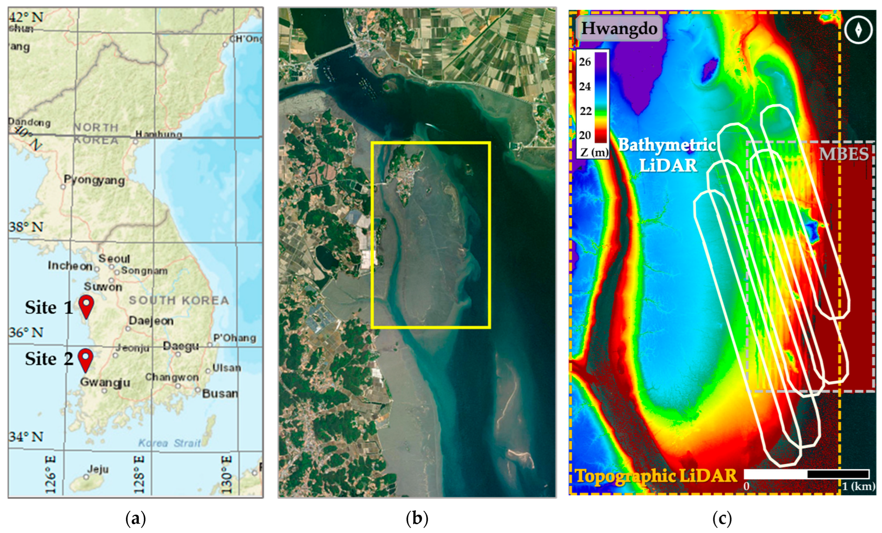
To assess the bathymetric performance of the proposed method in shallow and turbid conditions, we selected two test sites in tidal flats at Hwangdo and Gomso Bay, both with depths under 10 m. The test datasets were acquired by the Seahawk system in October 2023. Figure 1 shows the test site locations and the Seahawk survey area (outlined in white), while

Table 2. Summary of the test datasets.

	Location	Acquisition Date	Area (m2)	Maximum Depth (m)	Number of Waveforms	Turbidity
Site 1	Hwangdo, Taean-gun Chungcheongnam-do, Republic of Korea	15 October 2023	2,711,808	12	1,431,832	High
Site 2	Gomso Bay, Buan-gun, Jeonllabuk-do, Republic of Korea	22 October 2023	3,543,552	9.5	1,784,629	Very high

summarizes the datasets.

The Hwangdo tidal flat, located in Cheonsu Bay on the central coast of the Yellow Sea in Taean-gun, South Korea, features a diverse and complex geomorphology. Cheonsu Bay contains various geographic features, such as Anmyeondo Island and tidal channels, and is influenced by semidiurnal tides, with a maximum high tide of 6.33 m, a minimum low tide of 2.86 m, and an average tide of 4.59 m. Historically, the bay’s surface area decreased from 380 km² to approximately 180 km² due to reclamation projects. The Hwangdo tidal flat itself spans 1.65 km × 5.15 km, slopes gently, and consists of mud, mixed, and sand facies. Its highly varied topography includes tidal channels (0.02–2 m wide), cheniers, and sand shoals, all of which influence tidal flows and sediment patterns [29]. Water quality and turbidity at the site vary with season and tidal cycles. According to the Water Quality in Coastal Waters dataset (Korean Statistical Information Service, KOSIS), the mean suspended particulate matter (SPM) in 2023 was 10.90 mg/L, indicating a high level of turbidity [30].

Gomso Bay, a semi-enclosed, funnel-shaped macrotidal embayment on Korea’s central west coast, opens to the Yellow Sea via a broad entrance (5–8 km wide, 20 km long). The geology comprises Precambrian gneiss and Jurassic granite, flanked by mountainous regions rising 400–500 m to the north and south. Freshwater mainly enters through small rivers, including the Jujin Stream (29 km long, 229 km² basin) and Galgok Stream (21 km, 59 km² basin). The bay is characterized by extensive tidal flats covering approximately 106.2 km², with an average gradient of 0.081°. It experiences a macrotidal, semidiurnal tidal cycle, with high tides reaching up to 6.54 m and typical high tides averaging around 5.76 m [31]. The average surface SPM in 2023 was 89.20 mg/L, indicating a very high level of turbidity [30].

To objectively evaluate the experimental results, ATL and MBES data acquired at a similar time to the test data were utilized as the ground truth. The ATL data, which can only observe exposed ground, were acquired with a Terrain Mapper sensor at low tide on the same day as the Seahawk survey. As shown in Figure 1 (orange dashed box), even at low tide, tidal creeks and deeper waters remained submerged, making ATL surveying impossible in those areas. The MBES data were collected at high tide over three days, including the Seahawk survey date. Due to the minimum navigable depth of approximately 4 m and time constraints, the survey was limited to certain areas. Despite operating the vessel along the densest possible survey lines, the shallow depth restricted the swath width of the MBES sensor, resulting in unsurveyed areas between adjacent lines, as indicated in Figure 1 (gray dashed box). Thus, in tidal flats where water levels constantly fluctuate, conventional survey systems such as ATL or MBES leave unsurveyed and inaccessible regions. These challenging areas highlight the primary domain where ABL surveys can provide significant advantages.

3. Methods

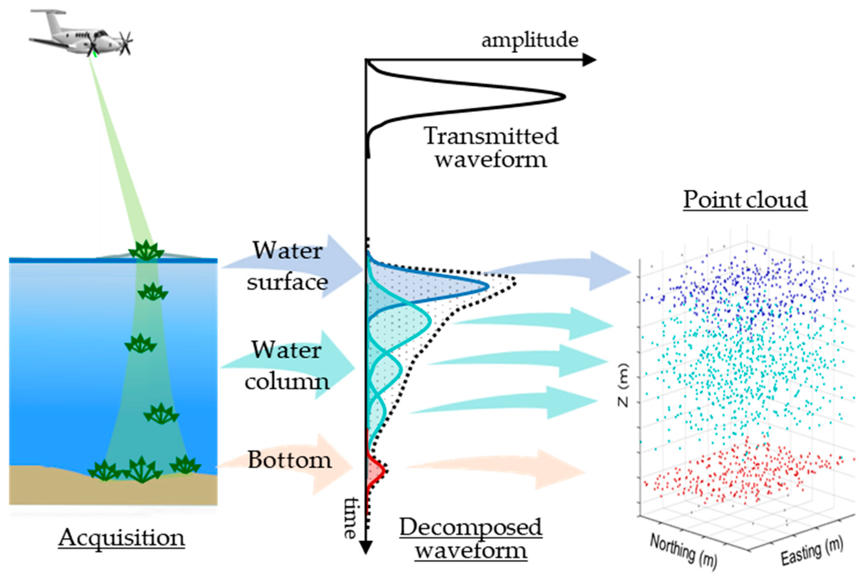
The green laser beam in ABL penetrates the water surface and propagates through the water column to the bottom. Its amplitude is rapidly attenuated by absorption, scattering, and refraction; if not fully extinguished, the backscattered signal returns to the receiver, revealing the water surface and bottom as peaks in the recorded waveform. A typical ABL waveform, therefore, consists of returns from the water surface, water-column backscatter, and bottom reflection, superimposed on noise. In processing, each waveform is decomposed into constituent components, the corresponding points are extracted, and a point cloud is generated (Figure 2).

The LiDAR waveform can be modeled as a convolution of a Gaussian pulse and a surface scattering function, and it is often represented as a Gaussian mixture model, as in Equation (1), where parameters such as amplitude ($A$), center ($\mu$), and standard deviation ($\sigma$) have physical meanings [32]. To decompose the waveform into Gaussian models, iterative optimization (e.g., Levenberg–Marquardt) is used, requiring careful selection of initial parameter values. In conventional Gaussian decomposition (CGD), the number of Gaussian components n is set to the number of initially detected peaks (local maxima). This intuitive approach is generally effective for ATL over land, where individual returns appear as distinct peaks.

$$\widehat{y}=\sum _{i=1}^n{A}_{i}exp\left(-{\displaystyle \frac{({t-{\mu }_i)}^2}{2{\sigma }_i^2}}\right)$$

(1)

However, ABL data often violate these assumptions because water-column backscatter produces left-skewed waveforms [23]. In very shallow water, surface and bottom returns frequently overlap and appear as a single peak [33,34], impeding accurate separation with traditional Gaussian methods. In highly turbid environments, enhanced underwater scattering and absorption substantially reduce the signal-to-noise ratio (SNR), hindering the transmission of bottom returns to the sensor [35]. These effects increase waveform asymmetry and further complicate the separation of surface and bottom reflections.

Given these challenges in shallow, turbid, and dynamically varying waters such as tidal flats, waveform processing techniques must be tailored to local conditions. Accordingly, we first analyze the properties of waveforms acquired under these environments and then propose an ABL waveform processing framework optimized for them. The approach builds on our previously developed progressive Gaussian decomposition (PGD), and the overall workflow is illustrated in Figure 3. The pipeline begins with noise removal to suppress background and random noise components, followed by signal range selection to isolate valid return segments. The refined waveform is then decomposed into Gaussian components through the adaptive PGD algorithm. Subsequently, waveform-derived features—such as amplitude, width, and area—are extracted and used for water-layer classification (surface, column, and bottom). The classified points are finally registered to generate the bathymetric point cloud.

3.1. Waveform Characteristics in Shallow and Turbid Waters

To analyze ABL waveform characteristics in tidal flat areas, we compared ABL (Seahawk) waveforms collected at the Hwangdo and Gomso Bay test sites with data acquired in clear waters off Korea’s east coast (mean SPM ≈ 4.5 mg/L in 2022). Relative to the clear-water site, waveforms from the turbid tidal flats often exhibited excessive or irregularly distributed random noise within portions of individual traces. For each waveform, the random noise level was estimated as the standard deviation of the no-signal range (0.10 µs; 160 bins) defined for the Seahawk system. In clear water, the random noise level averaged 91.03 ± 10.20 (max 235.40), whereas in the tidal flats it was 85.02 ± 19.34 (max 1264.33) at Hwangdo and 87.06 ± 16.62 (max 1291.14) at Gomso Bay, indicating strongly non-Gaussian behavior with occasional extreme bursts despite comparable means. This pattern is consistent with water column scattering under turbid conditions, which degrades the received signal’s SNR [22].

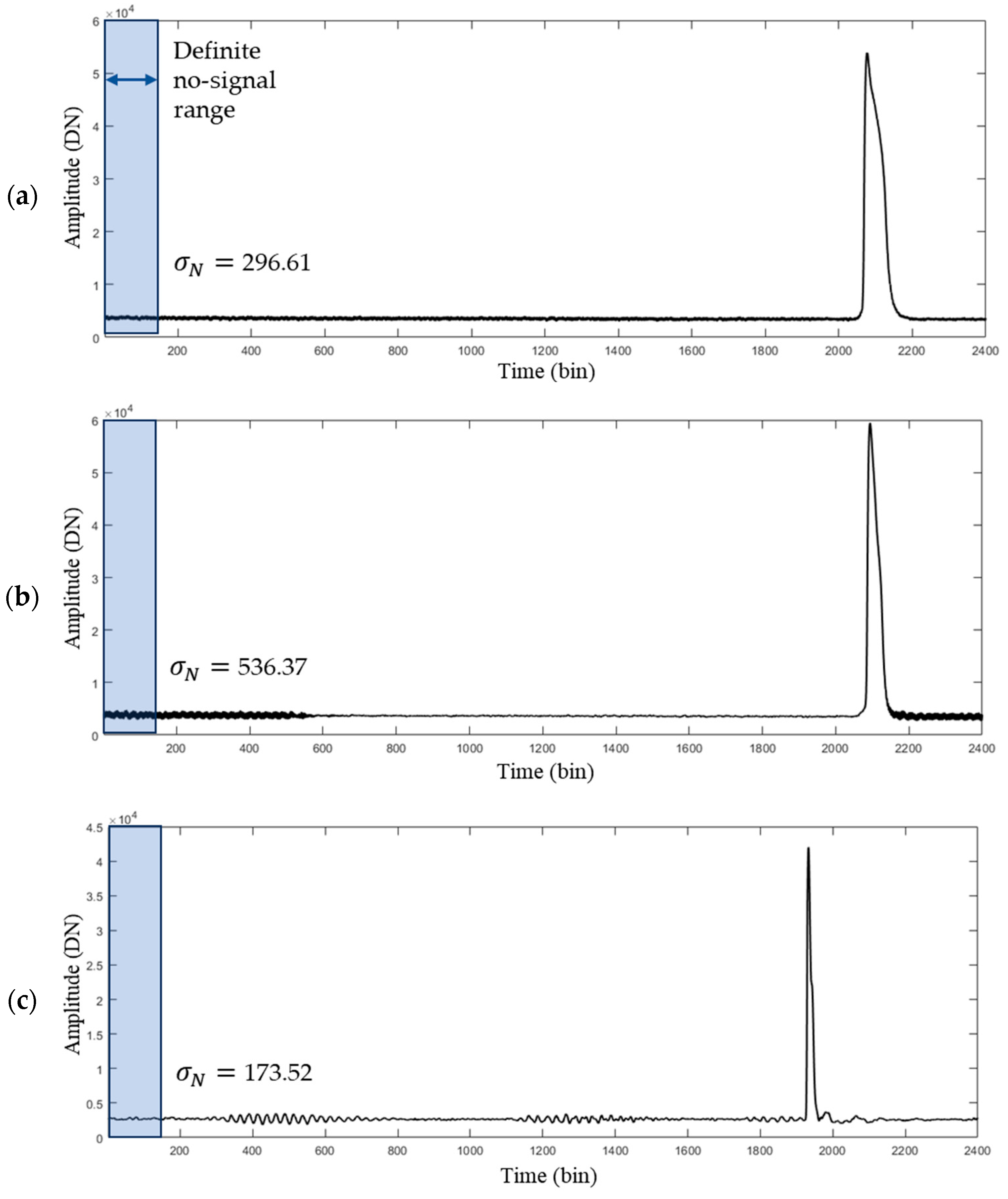
Figure 4 illustrates representative waveform types from turbid water with non-Gaussian random noise: (Figure 4a) large but uniformly distributed noise across the trace, which can often be mitigated with conventional low-pass filtering or adjacent-measurement-based waveform stacking techniques [36], which are designed to reduce ALB noise effects in shallow waters. However, (Figure 4b,c) locally inhomogeneous, intermittent noise that is not easily removed by low-pass filtering alone. In case (Figure 4c), automatic detection is particularly challenging because the no-signal range’s standard deviation is not itself large. Consequently, in turbid environments, it becomes critical to discriminate true reflection peaks from noise and to determine the actual signal range of the waveform with high fidelity.

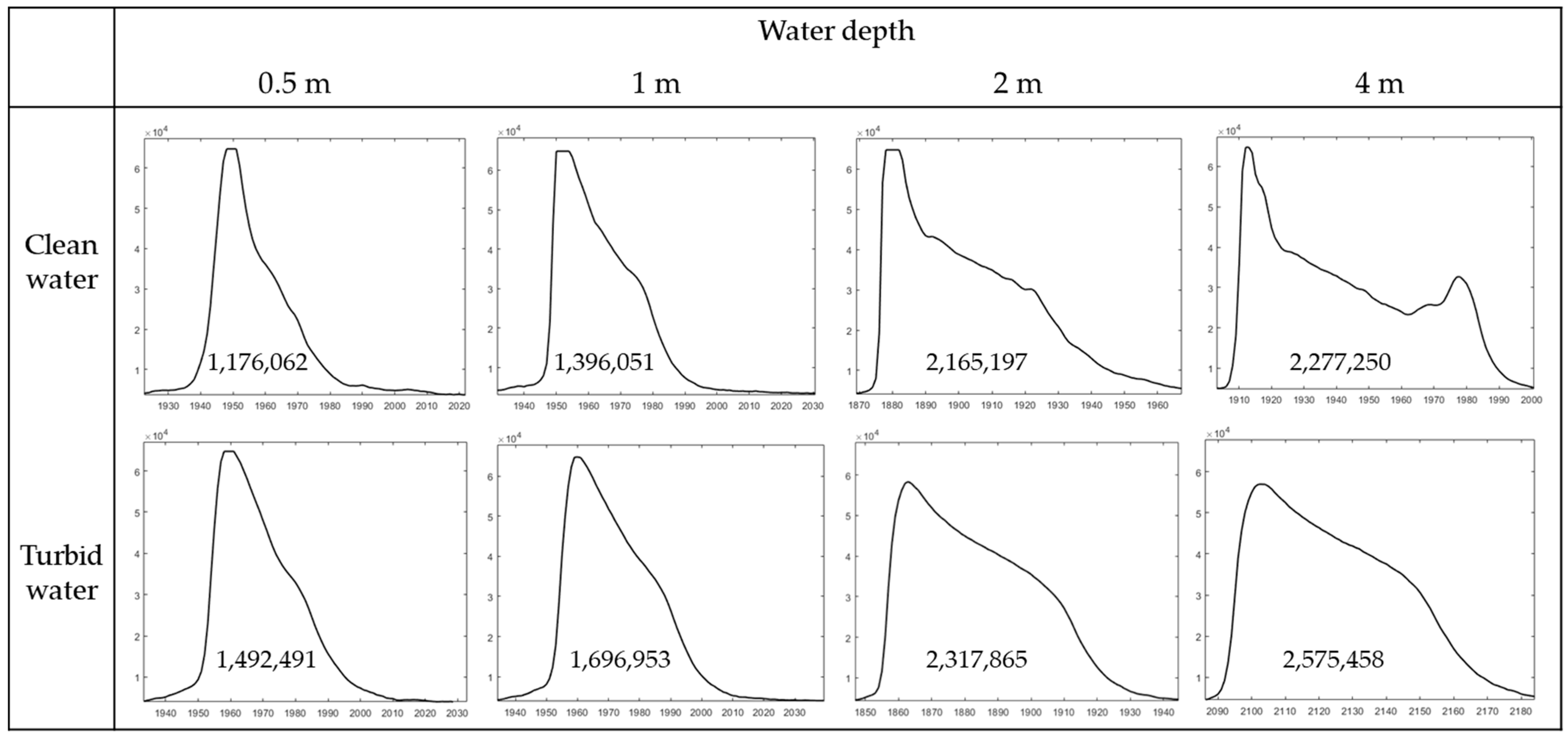
Figure 5 presents actual signal ranges of representative waveforms collected by the Seahawk system in shallow water under different turbidity conditions. Each column displays waveforms acquired at similar depths, with the annotated values denoting the integrated waveform area, which corresponds to the total return energy. (These examples are illustrative; actual waveform shapes may vary under different environmental conditions beyond just depth and turbidity.) At very shallow depths (approximately 0.5 m and 1 m), water surface and bottom reflections merge into a single peak in both clear and turbid waters, making it impossible to visually resolve a distinct bottom return. In clear water at deeper depths (2 m and 4 m), the water surface and bottom reflections become comparatively more distinct. In contrast, under turbid conditions, bottom returns remain inseparable from water surface and water column signals even at larger depths. This underscores the difficulty of isolating bottom components from ABL data in turbid environments, as well as the challenge of determining whether a waveform contains a true bottom return or only water surface and backscattered water column echoes.

Another important observation is that the waveform area varies with both turbidity and depth. Theoretically, the total integrated waveform area from a water column can be expressed as the sum of the cumulative water-column backscatter and the attenuated bottom reflection [37]:

$$A_{total}\propto {\displaystyle \frac{\beta }{2c}}\left(1-e^{-2c{z}_b}\right)+{\rho }_b{e}^{-2c{z}_b}$$

(2)

where $\beta$ is the backscatter coefficient, $c=a+b$ is the attenuation coefficient, $z_b$ is the bottom depth, and ${\rho }_b$ is the bottom reflectance. The first term represents the cumulative contribution of volume backscatter, which increases with depth before saturating, while the second term represents the bottom return that decreases exponentially with depth due to absorption and scattering. As shown in Figure 5, an analysis of shallow-water data (depths < 5 m) revealed that the total waveform area increases with depth in both clear- and turbid-water conditions. This trend can be explained by the cumulative contribution of volume backscatter along the water column and the enlargement of the laser footprint with increasing depth, which together outweigh the effects of attenuation losses. In addition, for the same depth, the total area tended to be larger in turbid waters than in clear waters. This analysis indicates that, in shallow waters, the restricted reflection angles at shallower depths limit the amount of energy that can be collected. In addition, in turbid waters, increased underwater backscattering can lead to greater energy being detected by the sensor compared with clear water conditions [38].

3.2. Preliminary Work

PGD [26] was designed to decompose diverse forms of ABL waveforms acquired under varying conditions—such as different water depths, turbidity levels, and the presence of underwater objects—by iteratively estimating undetected potential peaks and progressively refining the Gaussian mixture model. As a preprocessing step, PGD applies noise removal and valid signal range selection to improve computational efficiency and minimize outliers. Noise reduction was achieved by subtracting the mode (the most frequently occurring value) of each individual waveform to eliminate background noise, followed by Gaussian smoothing to suppress random fluctuations. For signal range selection, the algorithm identified the portion of the waveform where the signal amplitude exceeded a threshold determined from the standard deviation of the no-signal range, thereby isolating meaningful return signals for subsequent analysis. Then, the decomposition process begins with local maxima, or original peaks (OPs), which are used as initial parameters for Gaussian fitting via the Levenberg–Marquardt optimization algorithm. After fitting, estimated peaks (EPs) are compared with the OPs. If the time difference between them is within a specified threshold (τ) and the model achieves sufficient fitness (R² between the original waveform and the approximated Gaussian mixture model), the iteration terminates. Otherwise, additional potential peaks are selected—typically those most distant from the OPs—and added to the initial values of the decomposition in subsequent iterations. In this way, PGD adaptively determines the optimal number of Gaussian components rather than fixing it a priori. For detailed descriptions of PGD algorithms and parameterization, readers are referred to [26].

Despite these strengths, several limitations remain, particularly in shallow, turbid, and dynamic tidal flat environments (Section 3.1). First, the signal-range selection step can misclassify large-amplitude, spatially localized noise as a valid signal. Second, using R² as a termination criterion is not always appropriate for nonlinear ABL waveforms. The types of misdecomposition that can occur due to these causes will be discussed in more detail in the next section, Section 3.3. In addition, PGD focuses on decomposition itself and does not label each component by water layer type (surface, water column, bottom), which complicates robust seabed discrimination. These issues are exacerbated under high turbidity and overlapping returns, motivating the methodological refinements presented in the next section.

3.3. Adaptive Progressive Gaussian Decomposition

As a preprocessing step, the waveform undergoes noise removal and signal range selection. Background noise mainly originates from low-frequency noise generated by solar radiation and detector dark current, and is generally distributed uniformly throughout the waveform. Random noise is generally removed using low-pass filtering, and Gaussian filtering is applied for smoothing to minimize distortion of the original waveform:

$$y_t^{\prime }={\displaystyle \frac{1}{\sqrt{2\pi {\sigma }_G^2}}}{\sum }_{k=1}^w{y}_{k}exp\left(-{\displaystyle \frac{({t-k)}^2}{2{\sigma }_G^2}}\right),$$

(3)

where $y$ is the original waveform $y_t^{\prime }$ is the Gaussian filtered value at time $t$, $w$ denotes the number of waveform samples, and ${\sigma }_G$ is the standard deviation of the Gaussian distribution.

Next, it is important to determine the valid signal range to improve computational efficiency and prevent outliers. Since valid signals occupy only a small portion of the waveform, restricting the analysis to the signal range enhances processing efficiency and prevents large-amplitude noise in the non-signal range from being misinterpreted as a reflection echo. The start point and end point of the signal range are based on the standard deviation (${\sigma }_N$) and mean (${\mu }_N$) of the no-signal range. In the original PGD method, the start and end points of the signal range were simply defined as the positions where consecutive y-values increased or decreased by more than a multiple of the standard deviation. However, this approach can be inadequate when random noise occurs irregularly and excessively. To avoid misinterpreting noise as valid signals, we improved the signal range determination method as follows. The start point ($t_S$) of the valid signal range was determined as the point where the surface reflection signal begins, specifically where the signal amplitude (DN) exceeds ${\mu }_N$ and shows a significant increase (greater than $3{\sigma }_N$) over at least five consecutive bins, and the point with the longest continuous section ($R_{sig}$) was selected. Although specific implementations vary, many previous studies have similarly employed the $3\sigma$ criterion derived from the no-signal region to determine valid signal ranges in LiDAR waveform analysis [22,39,40]. The duration of five consecutive bins corresponds to 3.125 ns in the Seahawk system, and this threshold was empirically determined based on prior waveform analyses as a practical value that effectively suppresses random noise while still capturing the true onset of the signal in ABL waveforms. The end point ($t_E$) was determined as the point where the amplitude decreases below the DN value ($y_{t_S}^{\prime }$) at the start point.

$$\begin{array}{c}C\left(t\right):\left({y^{\prime }}_t>{\mu }_N\right)\bigwedge \left(\forall i\in \left\{1,2,\cdots ,5\right\},{y^{\prime }}_{t+i}-{y^{\prime }}_{t+i-1}>3{\sigma }_N\right),\\ R_{sig}=\mathrm{m}\mathrm{a}\mathrm{x}\left\{s|C\left(t\right)\bigwedge (\forall k\in \left\{0,1,\cdots ,s-1\right\},{y^{\prime }}_{t+k}\ge {y^{\prime }}_t)\right\},\\ t_S=min\left\{t|C\left(t\right)\right\},\mathrm{and}{t}_E=t_S+R_{sig}-1\end{array}$$

(4)

To ensure stable multi-Gaussian model fitting, the background noise value was set to $y_{t_S}^{\prime }$, so that the DN value at the start point becomes zero. The waveform was then adjusted by subtracting this value:

$$y_t^{*}={y^{\prime }}_t-{y^{\prime }}_{t_S}.$$

(5)

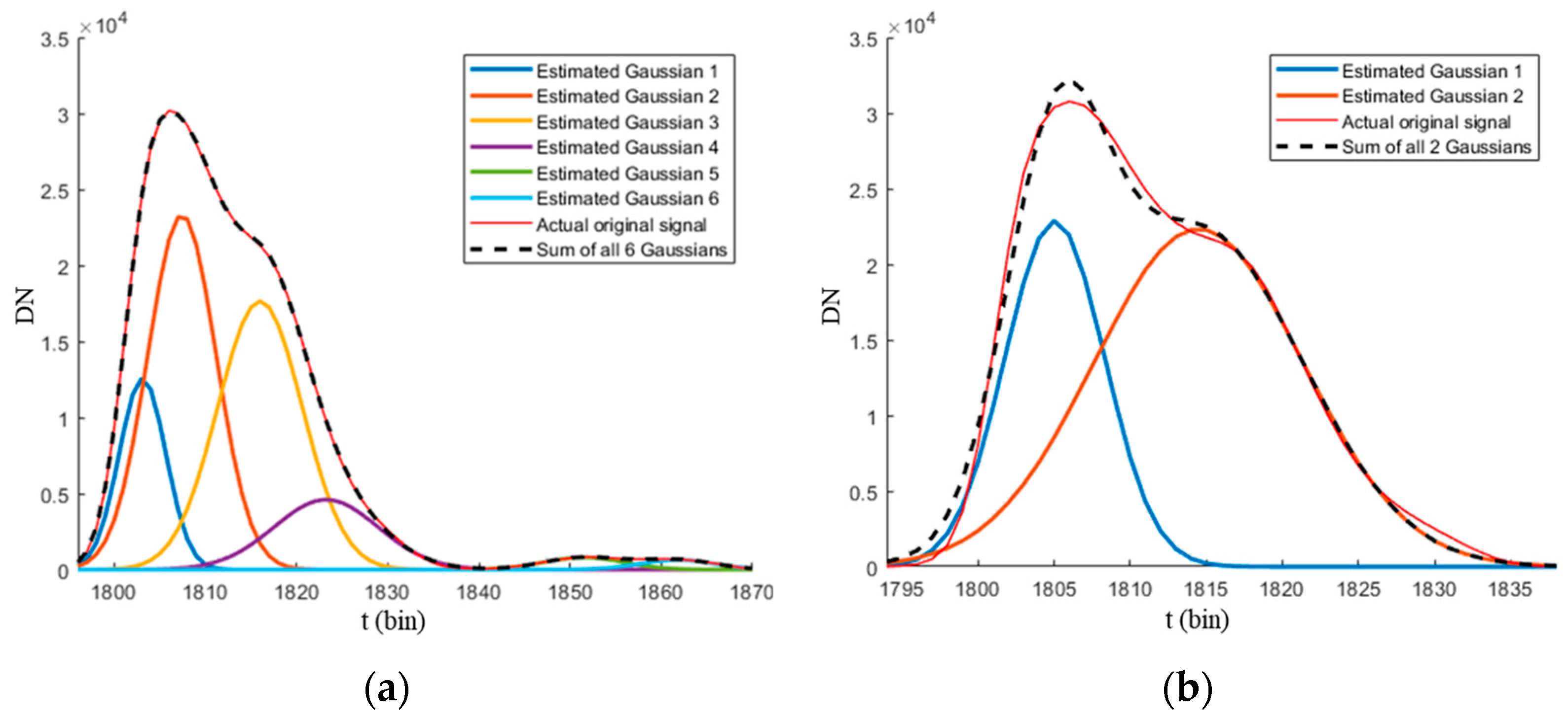
Figure 6 compares the results of signal range selection between the previous PGD method and the proposed approach for a waveform exhibiting excessive and irregular noise, as shown in Figure 4c. The PGD method (Figure 6a) included noise-dominated regions in the signal range, leading to incorrect decomposition and spurious components such as Estimated Gaussian Components 5 and 6. When these components are registered into points, they appear as outliers distributed below the actual seabed. In contrast, the proposed method (Figure 6b) selected an appropriate signal range, preventing unnecessary iterative computations and yielding stable and accurate decomposition results.

Basically, the decomposition process of APGD proceeds similarly to PGD. However, as noted earlier, R² used as a termination criterion is not suitable for assessing the fitness of nonlinear models. Instead, we adopted the maximum residual (${\mathsf{\epsilon }}_{\max }$) as the termination criterion based on residuals. The modified waveform decomposition process can be expressed in the following steps:

• Step $\mathrm{i}$. $r=1$; $S_{initial}=S_{OP}=\left\{{OP}_1,{OP}_2,\cdots ,{OP}_m\right\}$
• Step $\mathrm{i}\mathrm{i}$. $n=m+r-1$; Gaussian curve fitting with $S_{initial} \to S_{EP}=\left\{{EP}_1,{EP}_2,\cdots ,{EP}_n\right\}$
• Step $\mathrm{i}\mathrm{i}\mathrm{i}$. $\left\{\begin{array}{c}\left.if\begin{array}{c}\forall {∆t}_{OP}<\tau \\ and\\ {\mathsf{\epsilon }}_{\max }>T\end{array}\right]⟶stop,\\ otherwise⟶\left[\begin{array}{c}\begin{array}{c}\\ S_{PP}=\left\{{PP}_i|\begin{array}{c}{PP}_i={EP}_{mi},{EP}_{mi}\in S_{EP},\\ {∆t}_{{EP}_{mi}}=ith \underset{1\le k\le n}{\max }\left({∆t}_{{EP}_k}\right),1\le i\le r\end{array}\right\};\\ S_{initial}=S_{OP}\cup S_{PP};\end{array}\\ r=r+1;\\ Backtostep\mathrm{ii}.\end{array}\right.\end{array}\right.$

Figure 7 illustrates an example of the proposed APGD process. It shows the decomposition of a waveform recorded at a very shallow depth (0.8 m), where surface and bottom reflections overlap, resulting in only a single OP. In the first iteration (Figure 7a), the number of Gaussian components is set equal to the number of OPs, and each produces an estimated peak. In this case, the ${∆t}_{OP1}$ exceeded the threshold $\tau$, and ${\mathsf{\epsilon }}_{\max }$ was also above the limit, prompting another iteration. The results of the first fitting (Figure 7a) are equivalent to those of the CGD, demonstrating that CGD alone is insufficient for ABL waveforms. In the second iteration (Figure 7b), ${∆t}_{OP1}$ decreased compared with the threshold; however, ${\mathsf{\epsilon }}_{\max }$ still exceeded the limit. In the conventional PGD method, this step would satisfy both termination conditions—${∆t}_{OP1}$ below the threshold and R² above 0.95—thus ending the iteration. However, the shape of the Gaussian-fitted waveform (black dashed line) does not approximate the original waveform (red line) well enough. Since the proposed APGD method adopts ${\mathsf{\epsilon }}_{\max }$ as an additional termination criterion, it proceeds with further iterations. In this step, two EPs were selected as potential peaks for the initial value of the next iteration. The iterative fitting continued until both criteria were satisfied, producing the final Gaussian mixture models (Figure 7c).

3.4. Water-Layer Classification Based on Waveform Features

The waveform decomposition method is designed to separate return components but does not inherently identify the type of water column layer (i.e., water surface, water column, or bottom) associated with each component. Typically, the first return component in waveforms acquired over water bodies can be attributed to the water surface, while subsequent returns are generally assumed to originate from the water column (Figure 2). However, it remains necessary to determine whether the final return component represents an actual bottom reflection or a non-bottom return caused by subsurface scattering.

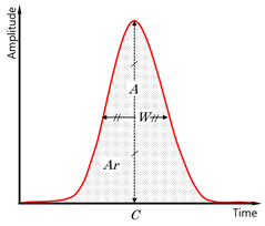
To address this, we employed waveform features to support bottom discrimination. Since each return component is modeled using Gaussian functions, various features can be derived for each component. In this study, we extracted features such as amplitude, center position, width, return number, number of returns, area, total area, area ratio, AW ratio, and normalized return (

Table 3. Definitions of waveform features.

Gaussian Model	Waveform Feature	Specifications
	Amplitude	$A$
	Center	$C$
	Width (FWHM)	$W$
	Return number	$N$
	Number of returns	$N_t$
	Area	$A_r=\sqrt{2}\pi AW$
	Total area	$\sum A_r$
	Area ratio	$R_A=A_r/\sum A_r$
	AW ratio	$R_{AW}=A/W$
	Normalized return	$R_R=N/N_t$

), and examined their relevance for bottom detectability.

To classify whether the last component corresponds to a bottom return, we compared feature distributions between bottom-detected and non-bottom-detected areas. Feature importance was calculated based on the total Gini impurity reduction at each split in the decision tree, as implemented in scikit-learn [41]. The resulting importance values in

Table 4. Feature importance for bottom-return classification.

Rank	Waveform Feature	Importance (%)
1	Total area	96.67
2	Width	2.28
3	AW ratio	0.86
4	Area ratio	0.16
5	Amplitude	0.02
⁞	⁞	0.00

represent the relative contribution of each feature to the overall classification performance, normalized to a total of 100%. Feature importance analysis indicated that total area was by far the most influential feature, with an importance score exceeding 96%. Total area, defined as the sum of all Gaussian component areas within a waveform, represents the total reflected energy and decreases due to energy losses caused by surface reflection, underwater scattering, and bottom reflection. In particular, bottom reflection losses are influenced by diffuse scattering, subsurface penetration, bottom reflectivity, and the angle of incidence. The analysis further revealed that the total area of bottom-detected waveforms was generally smaller than that of non-bottom signals. Therefore, an empirical threshold was applied to classify water layers based on this feature. As discussed in Section 3.1, however, waveform area is influenced by both turbidity and depth; thus, the threshold must be determined with consideration of these conditions in the study area.

4. Results

To validate the performance of the proposed ABL waveform processing technique, waveform data acquired from two test sites were used to compare bottom detection rates with those of existing software and to evaluate the accuracy of water-layer classification.

4.1. Seabed Detection Performance Evaluation

To evaluate the bathymetric performance improvement achieved by the proposed method, a comparative analysis was conducted against point clouds generated using Seahawk’s proprietary software (LBASSD) and the conventional PGD approach. The comparison of bottom-detected points across the methods clearly demonstrated the superior performance of the proposed APGD technique (

Table 5. Point extractability evaluation results of LBASSD and the proposed approach.

	Method	Total Point Cloud		Bottom Point Cloud		Seabed Coverage Ratio (%)
		Number of Points (pts)	Point Density (pts/m2)	Number of Points (pts)	Point Density (pts/m2)
Site 1	LBASSD	1,790,027	0.662	29,546	0.247	4.43
	PGD	2,883,646	1.064	1,000,003	0.531	69.49
	APGD	4,476,251	1.651	1,015,978	0.535	70.41
Site 2	LBASSD	3,274,429	0.926	5873	0.115	1.45
	PGD	3,997,545	1.128	1,086,119	0.491	62.2
	APGD	5,877,355	1.705	1,255,777	0.546	66.7

).

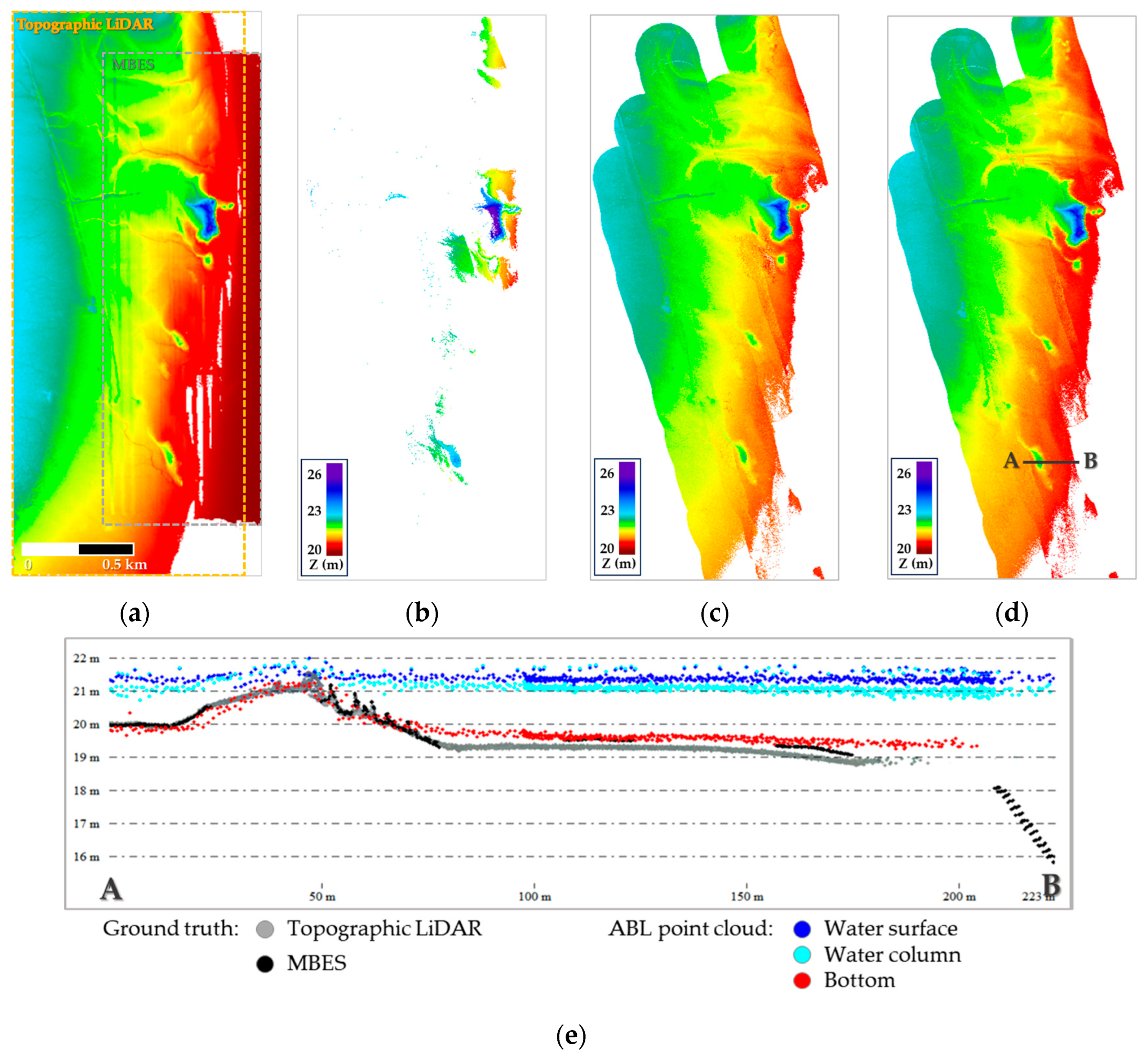
At Site 1 (Hwangdo), LBASSD extracted only 29,546 bottom-detected points, whereas the conventional PGD method extracted 1,000,003 bottom points. The proposed APGD method further improved extraction, yielding 1,015,978 bottom points. This represents a dramatic enhancement compared with LBASSD and a modest improvement over PGD. In terms of bottom point density, APGD reached 0.535 pts/m², an increase of more than double relative to LBASSD (0.247 pts/m²), and comparable to PGD (0.531 pts/m²). The seabed coverage ratio, a key metric indicating the proportion of the surveyed area with successfully detected bottom points, increased from only 4.43% (LBASSD) to 69.49% (PGD), and further to 70.41% with APGD. Figure 8 illustrates these differences at Site 1. Subfigures compare the ground-truth datasets (ATL and MBES), the LBASSD output, and the results from the PGD and the proposed approach. The LBASSD output (Figure 8b) shows sparse and incomplete bottom returns, while PGD and APGD (Figure 8c,d) capture the bathymetric structure with far greater continuity. The cross-section (Figure 8e) confirms that APGD recovers bottom points in close agreement with MBES ground truth, minimizing gaps in the LBASSD result.

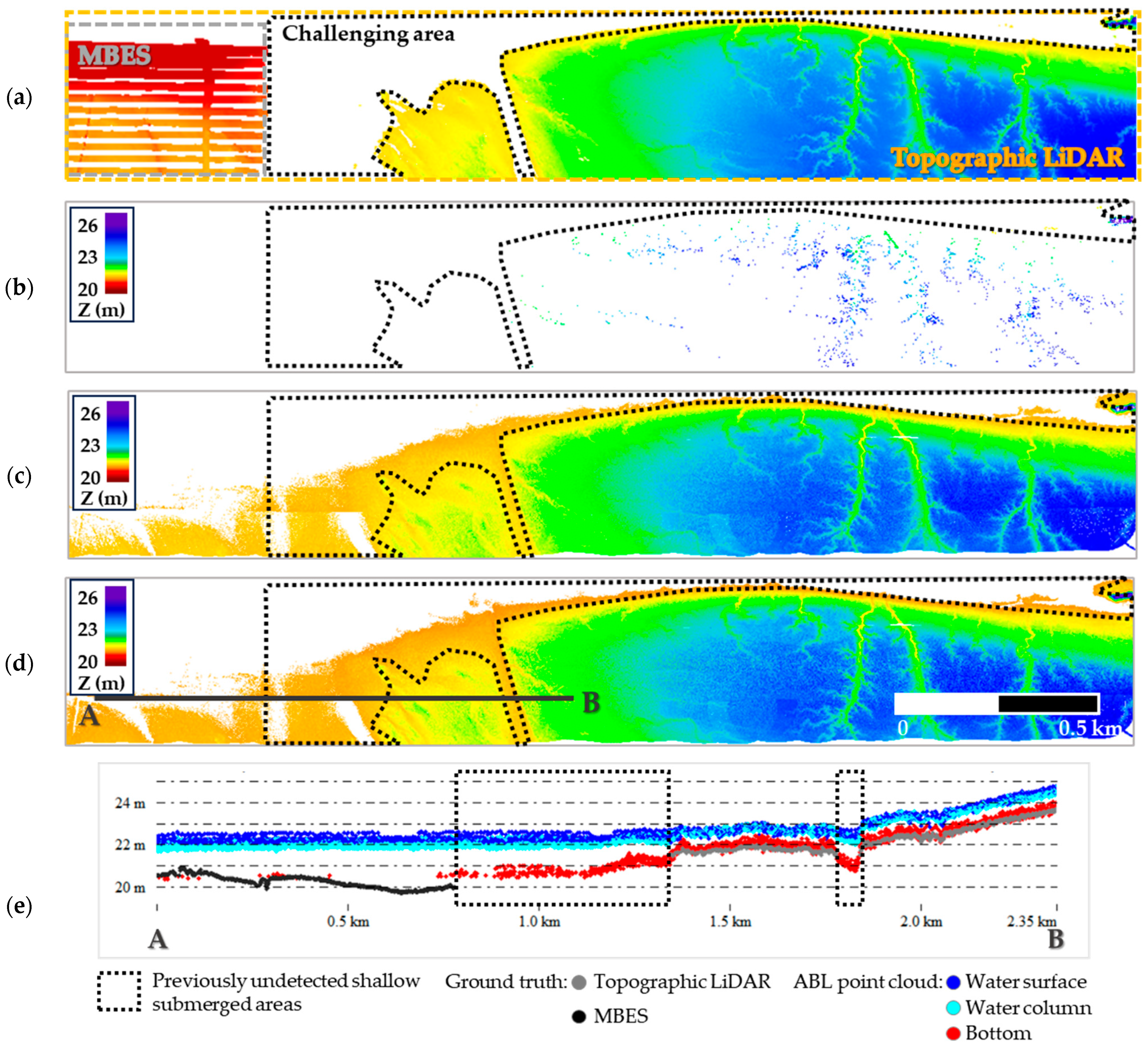
At Site 2 (Gomso Bay), where high turbidity severely limited bottom detection using LBASSD (5873 points; seabed coverage 1.45%), the advantage of APGD became more evident. PGD extracted 1,086,119 bottom points with a density of 0.491 pts/m² and a seabed coverage of 62.2%. APGD further improved these results, producing 1,255,777 bottom points with a density of 0.546 pts/m² and a seabed coverage of 66.7%. These findings highlight the ability of APGD to enhance bottom detection performance even under highly turbid conditions, significantly outperforming LBASSD and demonstrating measurable improvements over PGD in both point density and seabed coverage. Figure 9 provides visual evidence from Site 2. The challenging areas, where LBASSD failed to capture bottom returns (Figure 9b), are clearly resolved by APGD (Figure 9c,d). The cross-section along line AB (Figure 9e) shows that the APGD-derived bottom closely follows the ground truth and reveals previously undetected shallow submerged features. These results confirm the robustness of the proposed method in complex and turbid waters.

Finally, to evaluate the robustness of the proposed approach, the locational accuracy of the extracted seabed point cloud was assessed using in situ measurements acquired during low tide with the ATL system as ground truth.

Table 6. Comparison of the locational accuracy of bottom point clouds relative to ground-truth data and computational efficiency for the PGD and APGD methods at the two test sites.

	Method	Vertical Error (m)		Computational Efficiency (Waveforms/s)
		Mean	Standard Deviation
Site 1	PGD	0.216	0.226	1204.1
	APGD	0.093	0.187	1073.6
Site 2	PGD	0.101	0.151	1025.1
	APGD	0.069	0.186	1132.5

presents the locational accuracy of bottom point clouds derived from the two decomposition methods, PGD and APGD, at two test sites, along with their corresponding computational efficiency. At Site 1, the conventional PGD method yielded a mean vertical error (∆Z) of 0.216 m with a standard deviation of 0.226 m, whereas the proposed APGD method significantly reduced the mean error to 0.093 m and the standard deviation to 0.187 m. A similar trend was observed at Site 2, where the mean error decreased from 0.101 m (PGD) to 0.069 m (APGD). The standard deviation values were comparable between the two methods, with APGD showing slightly higher variation (0.186 m) compared to PGD (0.151 m). Overall, these results demonstrate that APGD provides a notable improvement in vertical accuracy of bottom point extraction compared with the conventional PGD approach, particularly in terms of reducing systematic bias in depth estimation. Moreover, the proposed method achieves reliable bathymetric performance that meets the accuracy requirements of the International Hydrographic Organization (IHO) Order 1b standard ($\sqrt{{0.5}^2+{(0.013\times depth)}^2}$ m; [42]).

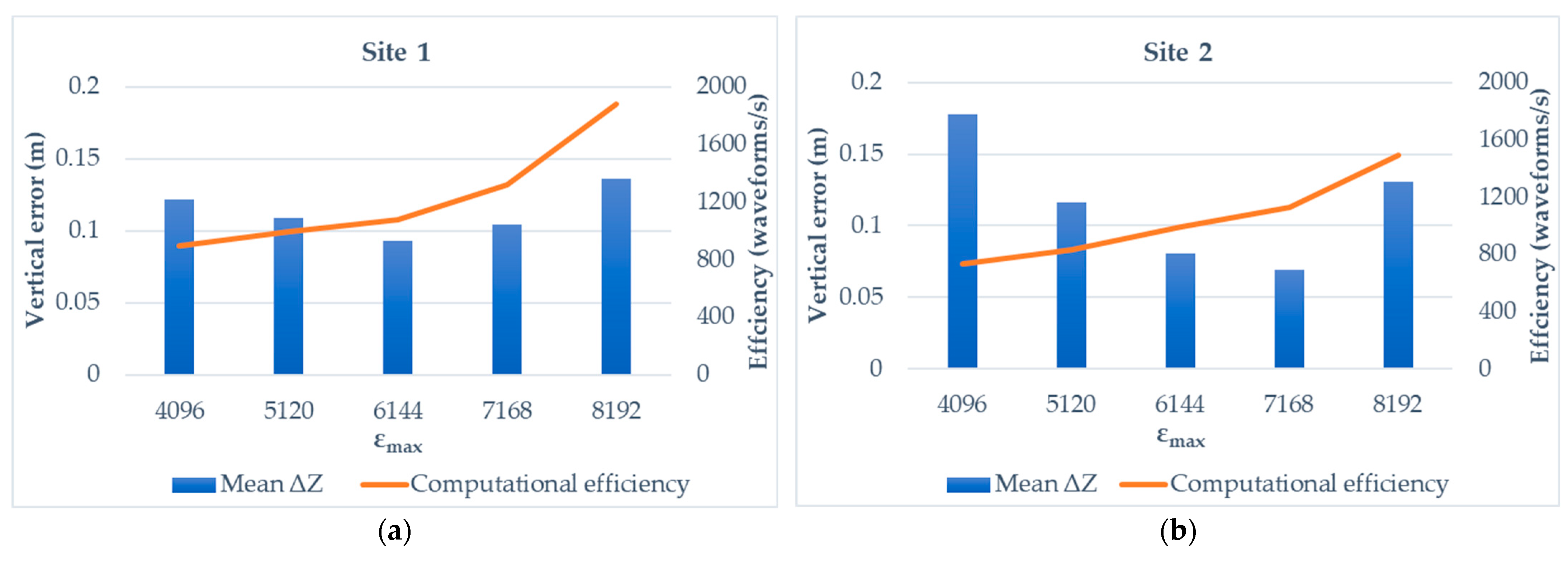
Computational efficiency (number of processing waveforms per second) was calculated to evaluate the calculation load with respect to different datasets. The test was implemented in MATLAB, and the experiments were conducted on a computer equipped with an Intel^® Core™ i5-7500 CPU (Intel Corporation, Santa Clara, CA, USA) and an NVIDIA GeForce RTX 3060 GPU (NVIDIA Corporation, Santa Clara, CA, USA). At Site 1, APGD was approximately 10.8% slower, while at Site 2 it was about 10.5% faster. This indicates that the variation in computational efficiency is primarily influenced by data characteristics such as noise and signal complexity rather than by algorithmic structure. Regardless of these minor differences in processing speed, APGD consistently achieved higher positional accuracy at both sites. Therefore, its overall accuracy-to-efficiency ratio can be considered more favorable compared with PGD. The locational accuracy and computational efficiency of APGD may vary depending on the termination-threshold parameter (ε_max), and this sensitivity is analyzed in detail in the Section 5.

4.2. Water-Layer Classification Evaluation

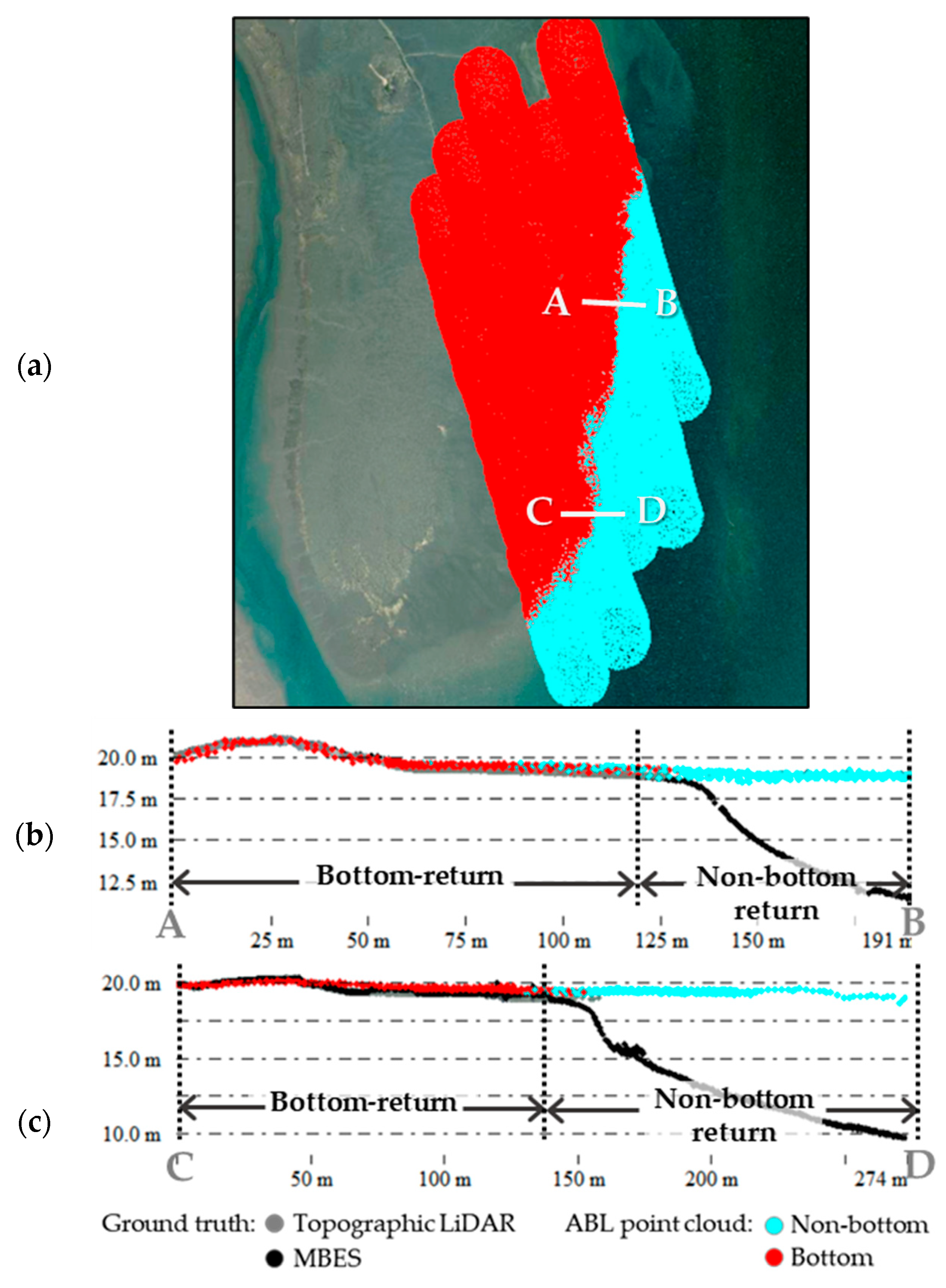
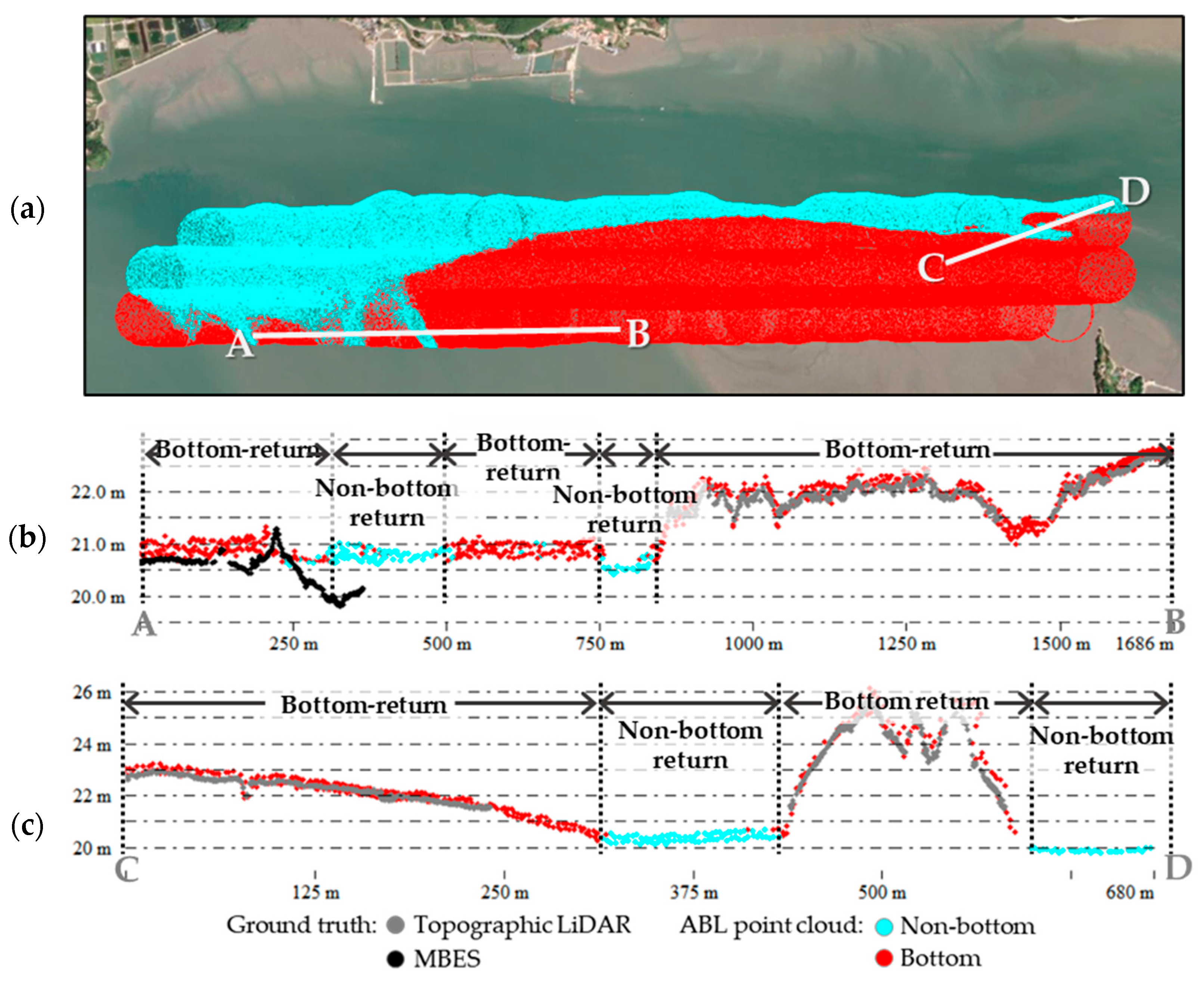
As described in Section 3.3, water layers can be labeled through rule-based classification using waveform features. To evaluate the performance of the proposed method, the classification accuracy of bottom and non-bottom returns was assessed using the last return point extracted from the ABL waveforms at both test sites. The total area thresholds applied for each site were 2,700,000 for Site 1 and 2,320,000 for Site 2, with a smaller value determined for Site 2, which exhibited relatively higher turbidity. As described in Section 3.1, the total area represents the sum of the cumulative water column backscatter and the attenuated bottom reflection. In shallow tidal flat environments, the contribution of cumulative water-column backscatter appears to dominate over the attenuation with increasing depth. The experimental results showed a bottom classification accuracy of 97.3% at Site 1 and 96.7% at Site 2. These accuracies were validated against ground truth datasets derived from ATL and MBES surveys. As shown in Figure 10 and Figure 11, the classification result at Site 1 (Figure 10a) demonstrates a clear spatial separation between bottom and non-bottom returns. The cross-sectional profiles along lines AB and CD (Figure 10b,c) further illustrate the method’s capability to distinguish bottom returns even in shallow and turbid waters. The classification result at Site 2 (Figure 11a), which includes a broader area with higher turbidity, confirms the effectiveness of the proposed method under more complex environmental conditions. In the cross-sectional views (Figure 11b,c), bottom returns (red) align well with the MBES-derived ground truth, while non-bottom returns (cyan) were appropriately excluded.

5. Discussion

This study introduced an enhanced waveform-processing technique optimized for ABL surveys in shallow and highly turbid tidal flat environments. By refining signal-range selection and introducing an adaptive termination criterion, the proposed APGD method substantially improved bottom-detection robustness compared with the manufacturer’s LBASSD software and the conventional PGD approach. Across the two test sites, seabed coverage ratios ranged from 66.7 to 70.4%, and bottom-classification accuracies reached 97.3% and 96.7%. Positional accuracy evaluations further demonstrated that APGD reduced mean depth errors relative to PGD, thereby minimizing systematic bias and satisfying the IHO Order 1b standard.

The sensitivity analysis of the termination parameter ε_max (Figure 12) revealed a trade-off between bathymetric accuracy and computational efficiency. As ε_max increases, the waveform fitting becomes less constrained, resulting in faster convergence and higher processing rates. However, excessive ε_max values lead to coarse approximations and greater underestimation of bottom depths, as indicated by the increased mean vertical error (ΔZ). Conversely, smaller ε_max values impose stricter residual thresholds, improving fitting precision but at the cost of computational efficiency and potential over-fitting in highly noisy conditions. This behavior was consistent across both test sites, but the influence of ε_max was more pronounced at Site 2, which exhibited higher turbidity. In turbid environments, the received waveform contains stronger subsurface scattering and irregular noise components, increasing the risk of over-fitting when ε_max is too small. Therefore, a, respectively higher ε_max threshold is required to ensure stable decomposition and to suppress spurious bottom points. According to the sensitivity analysis, ε_max was set to 6144 for Site 1 and 7168 for Site 2. It is important to note that the ε_max values presented in this study are not absolute but were empirically determined for the Seahawk system operated in Korean tidal flat conditions. The optimal ε_max value is expected to vary depending on sensor characteristics as well as environmental parameters, including turbidity and water depth. Accordingly, ε_max should be treated as an adaptive parameter rather than a fixed constant, and further calibration is required to optimize it under different survey settings.

Waveform-feature analysis further supported this adaptive perspective. Among all extracted features, the total area (representing cumulative signal energy) was identified as the most influential factor for distinguishing bottom returns, showing consistent differences between bottom-detected and non-bottom-detected waveforms. Because total area is affected by both turbidity and depth, empirical thresholds for classification should also be adjusted according to the optical and environmental conditions at the survey site. These findings collectively underscore the importance of environment-specific calibration when applying rule-based waveform classification methods.

Finally, visual analyses (Figure 8, Figure 9, Figure 10 and Figure 11) confirmed that APGD yields more continuous and reliable bottom surfaces under shallow and turbid conditions, and that classification results align closely with ATL and MBES ground truth. Overall, the proposed APGD waveform processing framework represents a scalable solution for high-resolution bathymetric mapping in complex waters, while also laying the groundwork for extended applications such as water–land boundary detection and submerged object identification.

While the proposed approach proved reliable, opportunities for further improvement remain. Turbidity can fluctuate substantially even within a single flight due to local tidal dynamics, making a single fixed threshold suboptimal for entire survey areas. Recent studies such as Chen et al. [43] suggest that adaptive or machine-learning-based strategies may further enhance generalizability, particularly in low-SNR or highly turbid environments. Additionally, simultaneous turbidity estimation offers important potential. Future work may involve mounting ABL and hyperspectral imaging systems on the same aircraft to collect concurrent datasets over tidal flats. As part of a related project, precise calibration of hyperspectral imagery—including atmospheric correction tailored to tidal flat conditions—and turbidity-mapping supported by in situ measurements are currently underway. Such integration would allow real-time observation of turbidity and water-optical properties during ABL acquisition, providing valuable auxiliary parameters for APGD and improving bottom-detection robustness in optically complex waters. In parallel, deep-learning models may be used to automate waveform-based classification and adaptive threshold tuning, allowing APGD to self-optimize across diverse turbidity and noise conditions.

Although APGD was developed using Seahawk ALB data, its processing logic is fundamentally system-independent and can be applied to other waveform-recording ALB sensors through modest recalibration of parameters such as τ and ε_max. To explore broader applicability and identify sensor-specific calibration requirements, validation experiments using another representative ALB system are currently in progress and will be reported in future work.

6. Conclusions

This study demonstrated that the proposed APGD method provides substantial improvements in bathymetric mapping performance for shallow and turbid tidal flat environments. By introducing adaptive termination criteria and refined signal-range selection, APGD enhances the stability of waveform decomposition, reduces spurious detections, and improves depth accuracy relative to both PGD and vendor software. APGD also produced more continuous and reliable bottom surfaces, with classification results closely aligned with ATL and MBES ground-truth data.

Although the thresholds and parameters presented in this study were empirically determined for the Seahawk system, the adaptive nature of APGD allows for transferability to other ALB sensors with appropriate recalibration. Future work will focus on integrating hyperspectral–ABL observations and machine-learning-based classification to further enhance generalizability and automate parameter selection. Overall, APGD represents a robust and scalable framework for high-resolution bathymetric mapping in complex tidal flat environments, with potential for extended applications such as detecting land–water boundaries and submerged objects.

References

1. Murray, N.J.; Phinn, S.R.; Clemens, R.S.; Roelfsema, C.M. The global distribution and trajectory of tidal flats. Nature 2019, 565, 222–225. [Google Scholar] [CrossRef]
2. Muylaert, R.L.; Friess, D.A.; Richards, D.R.; Alongi, D.M. Tidal flats as a significant carbon reservoir in global coastal ecosystems. Front. Mar. Sci. 2022, 9, 900896. [Google Scholar] [CrossRef]
3. UNESCO World Heritage Centre. Getbol, Korean Tidal Flats; Serial No. 1591; UNESCO: Paris, France, 2021; Available online: https://whc.unesco.org/en/list/1591/ (accessed on 2 November 2025).
4. Lee, J.; Kim, B.; Noh, J.; Lee, C.; Kwon, I.; Kwon, B.O.; Ryu, J.; Park, J.; Hong, S.; Lee, S.; et al. The first national scale evaluation of organic carbon stocks and sequestration rates of coastal sediments along the West, South, and East Coasts of South Korea. Sci. Total Environ. 2021, 793, 148568. [Google Scholar] [CrossRef]
5. Woo, K.S.; Chun, S.S.; Moon, K.O. Outstanding geoheritage values of the island-type tidal flats in Korea. Geoheritage 2020, 12, 8. [Google Scholar] [CrossRef]
6. Ryu, J.-H.; Lee, Y.-K. Remote sensing of Korean tidal flats. In Remote Sensing of the Asian Seas; Barale, V., Gade, M., Eds.; Springer International Publishing: Cham, Switzerland, 2019; pp. 221–235. [Google Scholar] [CrossRef]
7. Sun, J.; Tang, C.; Mu, K.; Li, Y.; Zheng, X.; Zou, T. Tidal flat extraction and analysis in China based on multi-source remote sensing image collection and MSIC OA algorithm. Remote Sens. 2024, 16, 3607. [Google Scholar] [CrossRef]
8. Gan, Z.; Guo, S.; Chen, C.; Zheng, H.; Hu, Y.; Su, H.; Wu, W. Tracking the 2D/3D morphological changes of tidal flats using time series remote sensing data in Northern China. Remote Sens. 2024, 16, 886. [Google Scholar] [CrossRef]
9. Parrish, C.E.; Magruder, L.A.; Perry, J.; Holwill, M.; Swinski, J.P.; Kief, K. Analysis and Accuracy Assessment of a New Global Nearshore ICESat-2 Bathymetric Data Product. Earth Space Sci. 2025, 12, e2025EA004391. [Google Scholar] [CrossRef]
10. He, J.; Zhang, S.; Cui, X.; Feng, W. Remote sensing for shallow bathymetry: A systematic review. Earth-Sci. Rev. 2024, 258, 104957. [Google Scholar] [CrossRef]
11. Kwon, J.; Kim, E. Estimation of shallow bathymetry using Sentinel-2 and random forest. J. Appl. Remote Sens. 2024, 18, 014522. [Google Scholar] [CrossRef]
12. Zheng, X.; Zhou, B.; Lei, H.; Jin, Y.; Su, Q. Mapping tidal flat topography using time-series Sentinel-2 images and ICESat-2 data: A case study in Cixi City. Ocean Coast. Manag. 2024, 256, 107278. [Google Scholar] [CrossRef]
13. Webster, T.; McGuigan, K.; Crowell, N.; Collins, K.; MacDonald, C. Optimization of data collection and refinement of post-processing techniques for Maritime Canada's first shallow water topographic bathymetric lidar survey. J. Coast. Res. 2016, 76, 31–43. [Google Scholar] [CrossRef]
14. Mandlburger, G.; Pfennigbauer, M.; Schwarz, R.; Flöry, S.; Nussbaumer, L. Concept and performance evaluation of a novel UAV-borne topo-bathymetric LiDAR sensor. Remote Sens. 2020, 12, 986. [Google Scholar] [CrossRef]
15. Bardi, R.; Cappietti, L.; Di Risio, M.; Romano, A.; Tancioni, L.; Taramelli, A. Evaluating short-term tidal flat evolution through UAV surveys: A case study in the Po Delta (Italy). Remote Sens. 2021, 13, 2322. [Google Scholar] [CrossRef]
16. Mulsow, C.; Rieke-Zapp, D.; Fritsch, D.; Neumann, A. Concepts for compensation of wave effects when measuring through water surfaces in photogrammetric applications. ISPRS Arch. Photogramm. Remote Sens. Spat. Inf. Sci. 2024, XLVIII-2, 289–295. [Google Scholar] [CrossRef]
17. Mallet, C.; Bretar, F. Full-waveform topographic lidar: State-of-the-art. ISPRS J. Photogramm. Remote Sens. 2009, 64, 1–16. [Google Scholar] [CrossRef]
18. Wang, C.; Li, Q.; Liu, Y.; Wu, G.; Liu, P.; Ding, X. A comparison of waveform processing algorithms for single-wavelength LiDAR bathymetry. ISPRS J. Photogramm. Remote Sens. 2015, 101, 22–35. [Google Scholar] [CrossRef]
19. Abdallah, H.; Bailly, J.S.; Baghdadi, N.N.; Saint-Geours, N.; Fabre, F. Potential of space-borne LiDAR sensors for global bathymetry in coastal and inland waters. IEEE J. Sel. Top. Appl. Earth Obs. Remote Sens. 2012, 6, 202–216. [Google Scholar] [CrossRef]
20. Abady, L.; Bailly, J.-S.; Baghdadi, N.; Pastol, Y.; Abdallah, H. Assessment of quadrilateral fitting of the water column contribution in lidar waveforms on bathymetry estimates. IEEE Geosci. Remote Sens. Lett. 2014, 11, 813–817. [Google Scholar] [CrossRef]
21. Ding, K.; Li, Q.; Zhu, J.; Wang, C.; Guan, M.; Chen, Z.; Yang, C.; Liao, J. An improved quadrilateral fitting algorithm for the water column contribution in airborne bathymetric lidar waveforms. Sensors 2018, 18, 552. [Google Scholar] [CrossRef]
22. Xing, S.; Wang, D.; Xu, Q.; Lin, Y.; Li, P.; Jiao, L.; Zhang, X.; Liu, C. A depth-adaptive waveform decomposition method for airborne LiDAR bathymetry. Sensors 2019, 19, 5065. [Google Scholar] [CrossRef]
23. Guo, K.; Xu, W.; Liu, Y.; He, X.; Tian, Z. Gaussian half-wavelength progressive decomposition method for waveform processing of airborne laser bathymetry. Remote Sens. 2018, 10, 35. [Google Scholar] [CrossRef]
24. Kang, C.; Lin, Z.; Wu, S.; Yang, J.; Zhang, S.; Zhang, S.; Li, X. Method to Solve Underwater Laser Weak Waves and Superimposed Waves. Sensors 2023, 23, 6058. [Google Scholar] [CrossRef]
25. Fang, J.; Liu, Z.; Sun, B.; Li, S.; Wu, W. Decomposition of full-waveform LiDAR data utilizing an adaptive B-spline-based model and particle swarm optimization. Measurement 2024, 235, 115002. [Google Scholar] [CrossRef]
26. Kim, H.; Jung, M.; Lee, J.; Wie, G. Progressive Gaussian decomposition of airborne bathymetric LiDAR waveform for improving seafloor point extraction. Appl. Sci. 2023, 13, 10939. [Google Scholar] [CrossRef]
27. Wu, L.; Chen, Y.; Le, Y.; Qian, Y.; Zhang, D.; Wang, L. A high-precision fusion bathymetry of multi-channel waveform curvature for bathymetric LiDAR systems. Int. J. Appl. Earth Obs. Geoinf. 2024, 128, 103770. [Google Scholar] [CrossRef]
28. Kim, H.; Tuell, G.H.; Park, J.Y.; Brown, E.; We, G. Overview of SEAHAWK: A bathymetric LiDAR airborne mapping system for localization in Korea. J. Coast. Res. 2019, 91, 376–380. [Google Scholar] [CrossRef]
29. Lee, J.-H.; Woo, H.J.; Jung, H.S.; Jang, Y.; Jeong, J.B.; Kim, K.; Seo, J.; Ryu, J.-H. Roles of exposure time and geochemical factors in the characteristics of the surface sediments of the Hwangdo tidal flat, Taean, Cheonsu Bay, West Coast of Korea. J. Mar. Sci. Eng. 2023, 11, 1697. [Google Scholar] [CrossRef]
30. Korean Statistical Information Service (KOSIS). Water Quality in Coastal Waters. Available online: https://kosis.kr/statHtml/statHtml.do?orgId=146&tblId=DT_MLTM_1742 (accessed on 2 November 2025).
31. Seo, J.; Koo, B.J. The sediment reworking of the mud shrimp Laomedia sp. (Crustacea: Laomediidae) with tidal conditions in the intertidal sediments of Gomso Bay, Korea. J. Mar. Sci. Eng. 2021, 9, 1251. [Google Scholar] [CrossRef]
32. Hofton, M.A.; Minster, J.B.; Blair, J.B. Decomposition of laser altimeter waveforms. IEEE Trans. Geosci. Remote Sens. 2000, 38, 1989–1996. [Google Scholar] [CrossRef]
33. Yang, F.; Qi, C.; Su, D.; Ding, S.; He, Y.; Ma, Y. An airborne LiDAR bathymetric waveform decomposition method in very shallow water: A case study around Yuanzhi Island in the South China Sea. Int. J. Appl. Earth Obs. Geoinf. 2022, 109, 102788. [Google Scholar] [CrossRef]
34. Guo, K.; Yang, Y.; Liu, B.; Li, S.; Wang, X.; Li, Z. Development of a single-wavelength airborne bathymetric LiDAR: System design and data processing. ISPRS J. Photogramm. Remote Sens. 2022, 185, 62–78. [Google Scholar] [CrossRef]
35. Kim, H.; Lee, J. Airborne bathymetric light detection and ranging waveform processing for digital elevation model construction of tidal flats on the west coast of Korea. Sens. Mater. 2024, 36, 4061–4075. [Google Scholar] [CrossRef]
36. Mader, D.; Westfeld, P.; Richter, K.; Maaß, H.; Richter, L. Volumetric nonlinear ortho full-waveform stacking in airborne LiDAR bathymetry for reliable water-bottom point detection in shallow waters. ISPRS J. Photogramm. Remote Sens. 2023, 204, 145–162. [Google Scholar] [CrossRef]
37. Guenther, G.C. Airborne Laser Hydrography: System Design and Performance Factors; National Oceanic and Atmospheric Administration: Washington, DC, USA, 1985. [Google Scholar]
38. Richter, K.; Mader, D.; Westfeld, P.; Maas, H.-G. Water turbidity estimation from LiDAR bathymetry data by full-waveform analysis—Comparison of two approaches. ISPRS Arch. Photogramm. Remote Sens. Spat. Inf. Sci. 2021, XLIII-B2-2021, 681–688. [Google Scholar] [CrossRef]
39. Jutzi, B.; Stilla, U. Range determination with waveform-recording laser systems using a Wiener filter. ISPRS J. Photogramm. Remote Sens. 2006, 61, 95–107. [Google Scholar] [CrossRef]
40. Chen, Y.; Le, Y.; Wu, L.; Li, S.; Wang, L. An assessment of waveform processing for a single-beam bathymetric LiDAR system (SBLS-1). Sensors 2022, 22, 7681. [Google Scholar] [CrossRef]
41. Pedregosa, F.; Varoquaux, G.; Gramfort, A.; Michel, V.; Thirion, B.; Grisel, O.; Blondel, M.; Prettenhofer, P.; Weiss, R.; Dubourg, V.; et al. Scikit-learn: Machine Learning in Python. J. Mach. Learn. Res. 2011, 12, 2825–2830. [Google Scholar]
42. USS S-44; IHO Standards for Hydrographic Surveys (S-44). International Hydrographic Organization (IHO): Monaco, 2020. Available online: https://iho.int/uploads/user/pubs/standards/s-44/S-44_Edition_6.1.0.pdf (accessed on 2 November 2025).
43. Chen, Y.; Wu, L.; Qian, Y.; Le, Y.; Yang, Y.; Zhang, D.; Wang, L. A novel strategy of full-waveform light detection and ranging bathymetry based on spatial gram angle difference field conversion and deep-learning network architecture. Remote Sens. Environ. 2025, 318, 114615. [Google Scholar] [CrossRef]
Figure 1. Test sites and data overview: (a) location map of the two test sites on the western coast of South Korea: Site 1 (Hwangdo) and Site 2 (Gomso Bay); (b) aerial image of Site 1 (Hwangdo tidal flat), showing the corresponding inset area. The yellow box indicates the test area presented in (c); (c) test dataset of Site 1: white lines indicate the test data from airborne bathymetric LiDAR (ABL; Seahawk), while the orange and gray dashed outlines represent airborne topographic LiDAR (ATL; Terrain Mapper) and multibeam echosounder (MBES) data used as ground truth, respectively; (d) aerial image of Site 2 (Gomso Bay tidal flat), showing the corresponding inset area. The yellow box indicates the test area presented in (e); (e) test dataset of Site 2: white lines indicate the test data from ABL (Seahawk), and the orange and gray dashed outlines denote ATL (Terrain Mapper) and MBES ground-truth data, respectively.
Remotesensing 17 03883 g001aRemotesensing 17 03883 g001b
Figure 2. Data flow of the ABL system, from laser interaction with water layers to point cloud generation. Colored points indicate different return types: blue (surface), cyan (water column), red (bottom).
Remotesensing 17 03883 g002
Figure 3. Workflow of the proposed ABL waveform processing framework. The process consists of sequential steps, including noise removal, signal-range selection, and waveform decomposition. Extracted waveform features are used for water-layer classification and point cloud generation.
Remotesensing 17 03883 g003
Figure 4. Examples of random noise types in ABL (Seahawk) waveforms in turbid water (tidal flat) and their random noise estimates: (a) large but uniformly distributed noise; (b) locally intermittent noise; (c) locally inhomogeneous noise.
Remotesensing 17 03883 g004
Figure 5. Comparison of ABL (Seahawk) waveforms in clear (top row) and turbid (bottom row) water at varying depths. The numeric values on each plot represent the integrated waveform area, representing the cumulative energy of the received signal.
Remotesensing 17 03883 g005
Figure 6. Comparison of signal range selection and waveform decomposition results for a waveform with irregular noise distribution (Figure 4c): (a) result of the previous method in progressive Gaussian decomposition (PGD; [26]); (b) result of the proposed method.
Remotesensing 17 03883 g006
Figure 7. Iterative steps of adaptive PGD (APGD): (a) first iteration with original peaks (OPs); (b) second iteration with the OPs and potential peaks; (c) final decomposition result.
Remotesensing 17 03883 g007
Figure 8. Bottom point extraction results at test Site 1: (a) ground truth (ATL and MBES), (b) LBASSD result; (c) PGD result; (d) proposed approach result; (e) cross-section of the line AB in (d).
Remotesensing 17 03883 g008
Figure 9. Bottom point extraction results at test Site 2: (a) ground truth (ATL and MBES), (b) LBASSD result; (c) PGD result; (d) proposed approach result; (e) cross-section of the line AB in (d).
Remotesensing 17 03883 g009
Figure 10. Bottom classification results for last return points: (a) results at Site 1; (b) cross-section along line AB in (a); (c) cross-section along line CD in (a).
Remotesensing 17 03883 g010
Figure 11. Bottom classification results for last return points: (a) results at Site 2; (b) cross-section along line AB in (a); (c) cross-section along line CD in (a).
Remotesensing 17 03883 g011
Figure 12. Sensitivity analysis of the termination threshold (εmax) for the APGD method at the two test sites: (a) Site 1 (Hwangdo) and (b) Site 2 (Gomso Bay). The blue bars represent the mean vertical error (ΔZ), and the orange line indicates the computational efficiency.
Remotesensing 17 03883 g012