Article

IFADiff: Training-Free Hyperspectral Image Generation via Integer–Fractional Alternating Diffusion Sampling

School of Mathematics and Statistics, Xidian University, Xi’an 710126, China
*
Author to whom correspondence should be addressed.
Remote Sens. 2025, 17(23), 3867; https://doi.org/10.3390/rs17233867
Submission received: 17 September 2025 / Revised: 17 November 2025 / Accepted: 27 November 2025 / Published: 28 November 2025

Highlights

What are the main findings?
  • Proposes an integer–fractional alternating diffusion strategy for high-fidelity, training-free hyperspectral image generation.
  • Enables free trade-off adjustment between texture richness and smoothness via the fractional order.
What are the implications of the main findings?
  • Delivers a plug-and-play framework to enhance existing diffusion solvers.
  • Bridges integer and fractional-order paradigms, extending the reach of generative models in hyperspectral analysis.

Abstract

Hyperspectral images (HSIs) provide rich spectral–spatial information and support applications in remote sensing, agriculture, and medicine, yet their development is hindered by data scarcity and costly acquisition. Diffusion models have enabled synthetic HSI generation, but conventional integer-order solvers such as Denoising Diffusion Implicit Models (DDIM) and Pseudo Linear Multi-Step method (PLMS) require many steps and rely mainly on local information, causing error accumulation, spectral distortion, and inefficiency. To address these challenges, we propose Integer–Fractional Alternating Diffusion Sampling (IFADiff), a training-free inference-stage enhancement method based on an integer–fractional alternating time-stepping strategy. IFADiff combines integer-order prediction, which provides stable progression, with fractional-order correction that incorporates historical states through decaying weights to capture long-range dependencies and enhance spatial detail. This design suppresses noise accumulation, reduces spectral drift, and preserves texture fidelity. Experiments on hyperspectral synthesis datasets show that IFADiff consistently improves both reference-based and no-reference metrics across solvers without retraining. Ablation studies further demonstrate that the fractional order α acts as a controllable parameter: larger values enhance fine-grained textures, whereas smaller values yield smoother results. Overall, IFADiff provides an efficient, generalizable, and controllable framework for high-quality HSI generation, with strong potential for large-scale and real-time applications.

1. Introduction

Hyperspectral image (HSI) refers to a type of image data that captures scene reflectance or radiation information across continuous and narrowly spaced wavelength ranges, characterized by simultaneously high spectral and spatial resolution. Unlike conventional RGB images, HSIs provide complete spectral curves over dozens or even hundreds of bands, thereby enabling the extraction of fine-grained material features at different wavelengths. This unique capability of joint spectral–spatial representation endows Hyperspectral image with extensive application potential in various fields. In recent years, with the rapid development of artificial intelligence, deep learning techniques have been widely applied to various HSI tasks, including denoising [1,2], super-resolution [3], and classification [4].
Nevertheless, despite the advantages of HSI, acquiring high-quality hyperspectral data remains challenging. Hyperspectral imaging systems are costly, data collection is time-consuming and sensitive to illumination and environmental conditions, and annotated ground truth is expensive to obtain. In addition, hyperspectral data are high-dimensional and exhibit strong spectral–spatial correlations, requiring efficient representation models to exploit their structure [5]. Consequently, the limited availability of HSI samples severely restricts large-scale dataset construction, often leading to overfitting and poor generalization in deep learning frameworks.
To alleviate these issues, data generation and augmentation have emerged as promising directions. By synthesizing new samples, training sets can be effectively expanded and model robustness improved. With the rapid progress of artificial intelligence, generative approaches such as Generative adversarial network (GAN) [6], Variational Auto-Encoders (VAE) [7], and Diffusion Models [8,9,10] have been increasingly employed for realistic HSI synthesis. These methods provide an efficient way to mitigate data scarcity and enable the creation of diverse, high-quality datasets, thereby supporting broader applications of HSI in practice.
Several recent studies have explored hyperspectral image (HSI) generation using diffusion models. Early methods such as Unmix-Before-Fuse (UBF) [11] and UnmixDiff [12] reconstruct full-spectrum HSIs from abundance maps, but their dependence on unmixing networks limits spectral fidelity and controllability. More recently, HSIGene [13] introduced a latent diffusion framework with ControlNet [14], enabling flexible conditional generation with reduced data requirements. Despite these advances, inference remains inefficient: high-dimensional HSI generation still requires tens to hundreds of steps using integer-order solvers like DDIM [15], making real-time or large-scale applications computationally prohibitive.
Since integer-order differentiation captures only local variations, integer-order diffusion solvers rely solely on the current state for each update, which can lead to cumulative errors such as spectral distortion and texture blurring. In contrast, fractional-order calculus introduces long-range dependencies by aggregating multiple historical states through non-integer derivatives, enabling stronger global consistency and error correction. However, fractional solvers are highly sensitive to the choice of order  α and may exhibit instability or oscillatory behavior in high-dimensional settings. Thus, neither integer- nor fractional-order updates alone are ideal: the former is stable but myopic, while the latter improves global coherence at the expense of robustness.
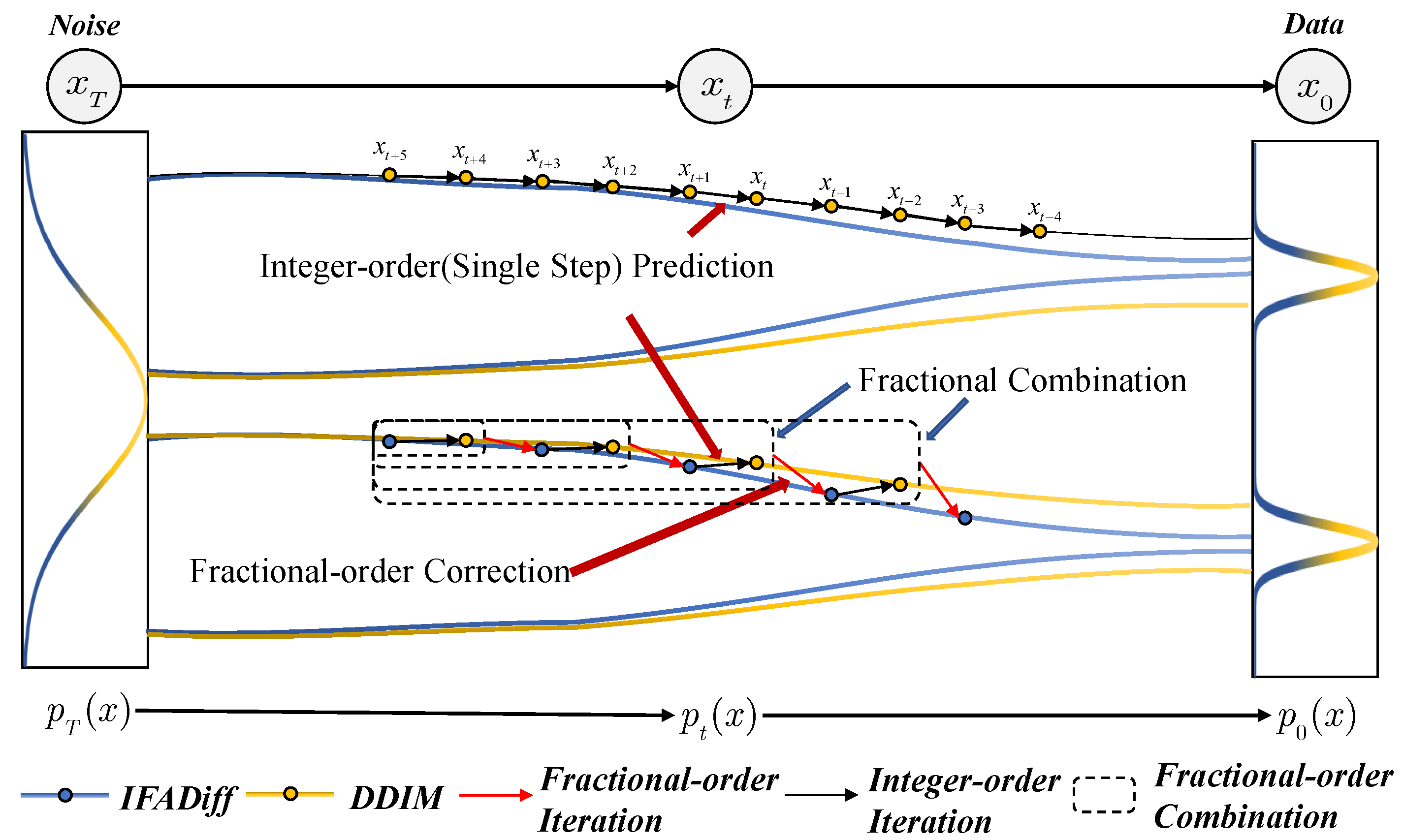
Motivated by these complementary properties, we propose Integer–Fractional Alternating Diffusion Sampling (IFADiff), a training-free inference-stage enhancement strategy that alternates between the two update types. As illustrated in Figure 1, IFADiff interleaves:
(1) Integer-order prediction. A standard deterministic diffusion update that ensures fast and stable forward progression.
(2) Fractional-order correction. A lightweight refinement step that integrates a decaying history of past states to enforce long-range consistency and recover fine spectral and spatial details.
This alternating mechanism combines the stability of integer-order prediction with the global regularization benefits of fractional-order modeling. It achieves reliable local updates during each prediction step. At the same time, it enhances long-range consistency across the entire sampling trajectory.
Being training-free, IFADiff operates entirely at the inference stage without any modification or retraining of the diffusion network. It builds upon existing pre-trained diffusion models and enhances sampling quality purely through an improved inference procedure. The fractional correction step is implemented as a numerical adjustment without introducing new learnable parameters, allowing seamless integration into existing solvers. This plug-and-play design enables flexible application across different diffusion architectures and ensures that the improvement in generation quality arises solely from algorithmic refinement rather than model retraining.
Main contributions of our work can be summarized as follows:
  • We propose an integer–fractional alternating time-stepping strategy, which combines the stability and efficiency of integer-order prediction with the long-range dependency modeling of fractional-order correction. This design avoids the error accumulation of purely integer-order solvers and the instability of purely fractional-order solvers, achieving a balanced and robust inference mechanism.
  • We introduce an efficient weighting scheme based on high-order approximations, enabling fractional-order corrections to be implemented with minimal overhead while improving spectral consistency and spatial fidelity in HSI generation.
  • IFADiff is formulated as a plug-and-play sampling framework that extends conventional integer-order solvers through fractional-order correction. The fractional order α serves as a controllable hyperparameter, allowing explicit trade-offs between stability, smoothness, and detail preservation according to task requirements.
  • The proposed method is entirely training-free and can be seamlessly integrated into existing diffusion solvers. Extensive experiments covering both unconditional and conditional HSI generation demonstrate consistent improvements across multiple baselines (e.g., DDIM, PLMS), highlighting the generality, scalability, and practical deployment potential of IFADiff.

2. Related Works

2.1. Hyperspectral Image Synthesis

Hyperspectral image (HSI) synthesis poses unique challenges due to the high spectral dimensionality and limited availability of labeled data. Early works reconstructed HSIs explicitly in the pixel domain through spectral unmixing or regression, but these methods suffered from accumulated modeling errors and poor generalization [16]. Subsequent unmixing-based generative models, such as UBF [11] and UnmixDiff [12], integrated diffusion processes into the unmixing pipeline to improve spectral consistency. Yet, their dependence on endmember estimation and the scarcity of training data still restrict spectral fidelity and controllability.
More recently, latent diffusion frameworks have emerged as a more flexible and data-efficient paradigm for HSI generation. Instead of reconstructing HSIs explicitly in the pixel domain, these methods perform generation entirely in a compact latent space and decode the results back to the hyperspectral domain using a pretrained variational autoencoder (VAE). This paradigm achieves higher data efficiency and flexibility, but inference remains time-consuming since it still depends on single-step integer-order updates. Moreover, these approaches mainly optimize model design or conditioning mechanisms, while the underlying numerical process of diffusion inference has received little attention. This design achieves higher data efficiency and better generalization, but still requires tens to hundreds of sampling steps for high-quality results, leaving inference efficiency the main bottleneck for real-time and large-scale applications.

2.2. Diffusion-Based Generative Models

Diffusion models (DMs) [8,9] have demonstrated remarkable capability in modeling complex data distributions through iterative denoising. Latent diffusion models (LDMs) [10] further improve efficiency by operating in compressed latent spaces, making them suitable for high-resolution or data-scarce domains such as remote sensing. Extensions like CRS-Diff [17] has enabled task-specific fine-tuning and multi-conditional control, achieving notable progress in generating realistic satellite and aerial imagery [18,19].
However, despite these advances, most existing diffusion frameworks rely on integer-order solvers such as DDIM [15] and PLMS [20] that require tens to hundreds of iterations to ensure stability. This results in high computational cost and limited temporal consistency across sampling steps, which remains a critical obstacle for efficient generative inference in remote sensing applications. Although recent fast solvers such as DEIS [21], DPM-Solver [22] and UniPC [23] have significantly reduced the number of sampling steps, they still rely on short-term multi-step coupling, where each update depends only on a few recent states. This local dependency limits their ability to capture long-range temporal correlations, often leading to spectral inconsistency or texture artifacts in high-dimensional data such as hyperspectral imagery. Moreover, these solvers involve multiple network evaluations per step and remain sensitive to noise or step-size variations, which restricts their efficiency and stability under complex sampling dynamics.
From a numerical perspective, integer-order solvers rely solely on the most recent state for each update, making the sampling trajectory inherently local and prone to cumulative error propagation. In contrast, fractional-order formulations naturally incorporate multiple historical states through a decaying weighting mechanism, enabling the model to retain long-range memory across the diffusion trajectory. This memory effect smooths the evolution of latent representations, mitigates noise amplification, and enhances spectral and spatial consistency, which are particularly desirable properties for hyperspectral image generation where both fine detail preservation and global spectral smoothness are critical. Therefore, we extend the conventional integer-order sampler in diffusion models to a fractional-order formulation that can more effectively exploit historical information and improve overall sampling stability.

3. Preliminary

3.1. Diffusion Models

Diffusion models aim to learn the data distribution q ( x 0 ) by iteratively denoising samples drawn from a standard normal distribution. A forward process gradually adds noise to the data, while a reverse process reconstructs the clean sample. Early diffusion probabilistic models (DPMs) adopted discrete Markov chains, where each step models a conditional transition between noisy latent variables.
Song et al. [24] extended DPMs to continuous time via stochastic differential equations (SDEs). However, discretized SDE sampling typically requires many steps due to injected stochasticity, as in DDPM with T = 1000  [8]. To reduce this cost, Song et al. [24] derived the probability flow ODE (PF-ODE), which shares the same marginals as the SDE:
d x t = f ( t ) x t 1 2 g 2 ( t ) x log q t ( x t ) d t , x t q ( x t ) ,
where eliminating stochasticity enables PF-ODE to converge with far fewer steps. Using a single-step RK45 solver [25,26], high-quality samples can be obtained with only 60 function evaluations, compared with 1000 in DDPM.
Recent works focus on discrete ODE-style samplers that require fewer function evaluations (NFEs), such as DDIM [15] and DPM-Solver [22]. DDIM relaxes the Markov assumption in DDPM and proposes the following update:
x t δ = α t δ x t 1 α t ϵ θ ( x t , t ) α t + 1 α t δ σ t 2 ϵ θ ( x t , t ) + σ t ϵ t ,
where σ t = η ( 1 α t δ ) / ( 1 α t ) 1 α t / α t δ . Setting η = 1 retrieves DDPM, while η = 0 recovers the deterministic ODE form of DDIM, which enables high-quality sampling with substantially fewer steps. However, DDIM is a first-order method with limited accuracy, motivating the use of higher-order numerical solvers.
Following this idea, PLMS [20,27] introduces a fourth-order Adams–Bashforth multistep update into the DDIM framework, significantly improving sampling accuracy and efficiency. Its update rules are
e t = ϵ θ ( x t , t ) ,
e t = 1 24 ( 55 e t 59 e t δ + 37 e t 2 δ 9 e t 3 δ ) ,
x t + δ = ϕ ( x t , e t , t , t + δ ) ,
where the DDIM transition function ϕ ( · ) is given by
x t + δ = ϕ x t , ϵ t , t , t + δ = α t + δ α t x t α t + δ α t α t 1 α t + δ α t + 1 α t α t + δ ϵ t .
Compared with the gradient estimation in DDIM, PLMS provides (i) higher estimation accuracy and (ii) improved runtime efficiency, enabling high-quality generation with substantially fewer NFEs. This makes PLMS particularly attractive for real-time hyperspectral image synthesis and other time-sensitive diffusion applications.

3.2. Fractional-Order Differential

Fractional calculus extends classical differentiation to non-integer orders, enabling the modeling of systems with long-range memory and non-local dependencies [28,29]. Unlike a first-order derivative that depends only on the current state, a fractional derivative aggregates multiple past states with gradually decaying influence, making it suitable for processes exhibiting hereditary behavior or anomalous diffusion.
Among existing definitions, the Grünwald–Letnikov (G–L) form is particularly convenient for discrete-time computation. Given a function f ( t ) , its α -order G–L derivative is defined as
D t α f ( t ) = lim s 0 1 s α k = 0 ( t a ) / s ( 1 ) k α k f ( t k s ) ,
where α k denotes the generalized binomial coefficient and s denotes the timestep. When α = 1 , Equation (7) reduces to the standard first-order derivative.
For numerical use, the G–L operator is commonly approximated by a truncated discrete series:
D t α f ( t ) k = 0 K w k ( α ) f ( t k ) , w k ( α ) = ( 1 ) k α k ,
where the coefficients w k ( α ) follow a power-law decay, and the truncation coefficient K controls the trade-off between accuracy and computational cost.
To improve accuracy, high-order variants of the G–L scheme have been developed [30,31,32]. Using the recurrence relation of the G–L coefficients g k ( α ) , a fourth-order accurate weighted formulation can be written as
w 0 ( α ) = α 2 + 3 α + 2 12 g 0 ( α ) , w 1 ( α ) = α 2 + 3 α + 2 12 g 1 ( α ) + 4 α 2 6 g 0 ( α ) , w k ( α ) = α 2 + 3 α + 2 12 g k ( α ) + 4 α 2 6 g k 1 ( α ) + α 2 3 α + 2 12 g k 2 ( α ) , k 2 ,
where the expression provides a stable and symmetric discretization, where each w k ( α ) controls the contribution of the k-step historical state f t k . We adopt this fourth-order approximation to efficiently capture fractional long-memory behavior during diffusion sampling.
The difference between integer- and fractional-order updates becomes evident from this discrete form. Integer-order samplers such as DDIM, PLMS, DPM-Solver++ [33], and UniPC [23] rely only on one or a few recent states, exhibiting inherently short-memory behavior. In contrast, a fractional-order operator aggregates a long tail of historical states { f t k } via smoothly decaying weights w k ( α ) , naturally introducing long-term dependencies.
However, purely fractional updates may converge slowly when α < 1 or become unstable when α > 1 , especially in high-dimensional settings. This motivates the hybrid design adopted in our method, which leverages the long-memory advantages of fractional modeling while maintaining stability and computational efficiency.

4. Proposed Method

Existing integer-order diffusion solvers rely on only one or a few recent states, causing short-memory updates that accumulate errors and degrade fine spectral and structural details. Pure fractional-order schemes incorporate long-range history but are highly sensitive to the choice of  α . To address these complementary limitations, we propose IFADiff, an alternating integer–fractional sampling strategy with a predictor–corrector structure: integer-order steps provide stable and efficient predictions, while fractional-order steps introduce memory-aware corrections.
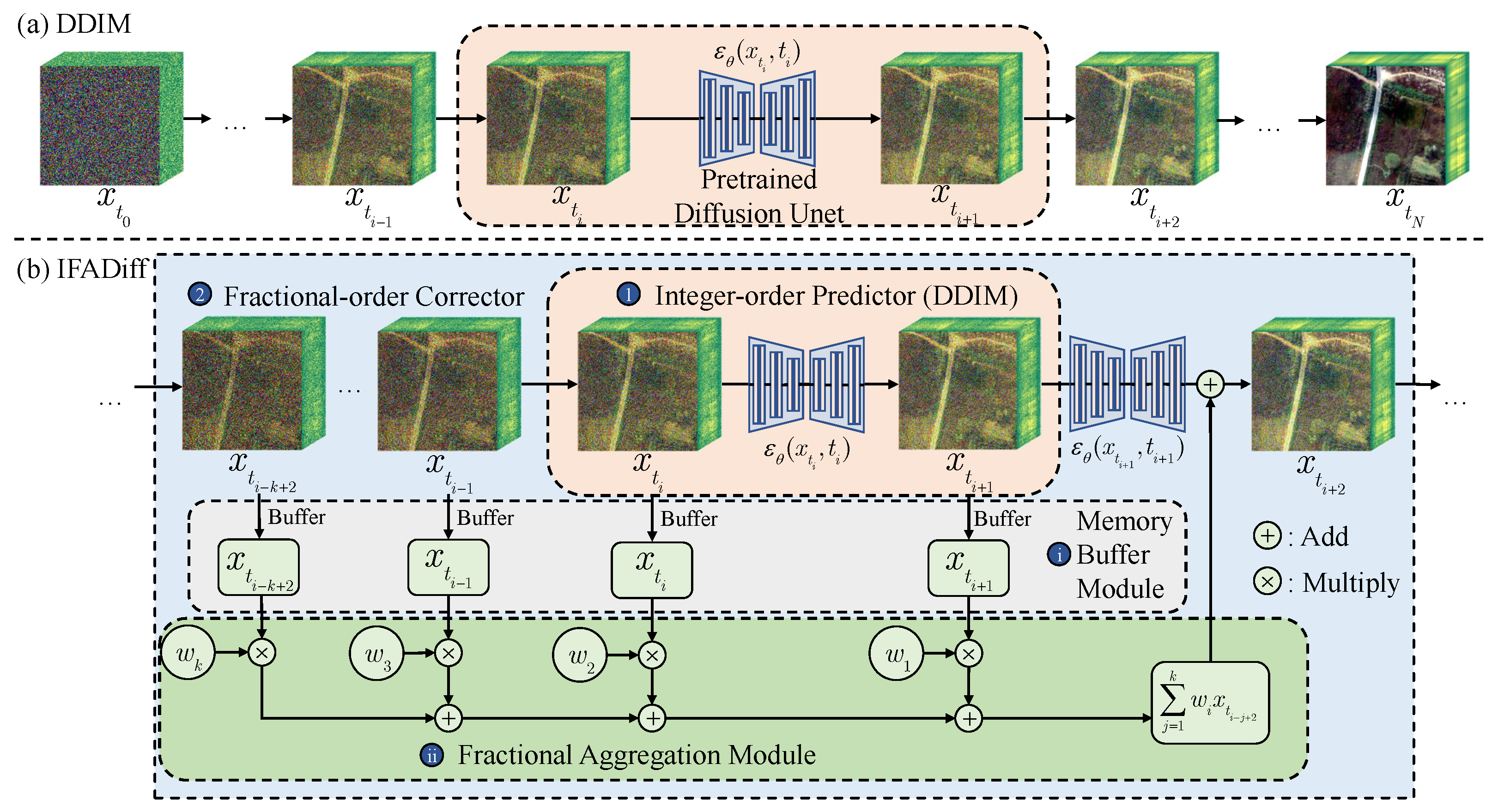
By interleaving prediction and correction, IFADiff achieves stable convergence and improved spectral–spatial fidelity. Figure 2 summarizes the workflow, where each step first applies the DDIM-based integer-order predictor and then performs a fractional-order correction. The memory buffer and its buffer nodes provide access to past states, and the fractional aggregation module integrates these states through weighted combinations. The adaptive α further adjusts the strength of the correction across sampling steps. Together, these components capture long-range dependencies and guide the generation toward more consistent hyperspectral outputs.

4.1. Integer–Fractional Alternating Diffusion

4.1.1. Integer-Order Prediction

During the inference stage, we first specify a discrete time grid { t i } i = 0 N between the start time t 0 and the terminal time t N . For two consecutive timesteps t i and t i + 1 on this grid, we perform a standard integer-order update. This update can be implemented using the first-order DDIM scheme, and is written as
x t i + 1 = x t i + Δ t i i + 1 · ϕ x t i , ϵ θ ( x t i , t i ) , t i , t i + 1 ,
where x t i R H × W × C denotes the generated sample at timestep t i . In hyperspectral image (HSI) generation, the channel dimension C can reach several tens or even hundreds, which makes error accumulation more pronounced compared to natural RGB images. The term ϵ θ ( x t i , t i ) represents the noise predicted by the pretrained diffusion model, ϕ ( · ) denotes the state-transition function defined by DDIM from Equation (6), and Δ t i i + 1 = t i + 1 t i is the step size. This step efficiently provides a provisional estimate of the next state with low computational cost.
Note that ϕ ( · ) here corresponds to a single-step DDIM integer-order update, i.e., Equation (6) applied from t i to t i + 1 . If we replace the instantaneous noise prediction ϵ θ ( x t i , t i ) with a higher-order multi-step estimate ϵ t i computed using the PLMS formulas in Equations (3) and (4), the same structure naturally recovers the PLMS scheme. Thus, this integer-order prediction provides a unified formulation in which DDIM and PLMS differ only in how the noise term is estimated, while the state-transition function ϕ ( · ) remains compatible with the fractional-order correction that will be introduced in the next subsection.

4.1.2. Fractional-Order Correction

To incorporate long-range memory and mitigate error propagation, we design a fractional-order correction that follows each integer-order update. This correction leverages historical states to refine the evolution trajectory rather than relying solely on the most recent step, thereby providing better global consistency. Specifically, inspired by the fractional derivative, which naturally embeds memory effects into differential operators, the diffusion dynamics can be generalized to the following fractional-order ordinary differential equation (ODE):
D t α x ( t ) = h θ ( x t , t ) d t , t [ 0 , 1 ] ,
where α is a fractional order that controls the balance between local and historical influences.
For numerical computation, we employ the G–L approximation to discretize the system:
D t α x ( t k ) 1 s α i = 0 k w i ( α ) x t k i ,
where { w i ( α ) } i = 0 k + 1 are G–L coefficients derived from Equation (9), which ensure higher accuracy while remaining computationally efficient. In practice, since the G–L weights w i ( α ) decay approximately following a power-law ( w i ( α ) i α 1 ), the contribution of distant historical states rapidly diminishes. Therefore, the summation can be safely truncated to a finite memory length K, i.e.,
D t α x ( t k ) 1 s α i = 0 K w i ( α ) x t k i , K k ,
the truncation effectively limits the number of stored feature maps, ensuring both efficiency and numerical stability. As shown in Table 1, the cumulative weighting error decreases rapidly as K increases, and becomes smaller than 10 3 once K 10 .
Building on the integer-order update that advances the state from t i to t i + 1 , we now derive a fractional-order correction that refines the transition over the enlarged interval [ t i , t i + 2 ] , using x t i + 1 as an intermediate predictor. To this end, we apply the truncated G–L approximation at timestep t i + 2 on the same discrete grid { t i } i = 0 N . Assuming a local step size h between t i and t i + 2 , the fractional derivative at t i + 2 can be approximated as
D t α x ( t i + 2 ) 1 s α j = 0 n w j ( α ) x t i + 2 j , n = min { K , i + 1 } ,
by evaluating the fractional ODE in Equation (11) at t i + 2 , we obtain
D t α x ( t i + 2 ) = h θ ( x t i + 2 , t i + 2 ) .
In practice, the drift term h θ ( x t i + 2 , t i + 2 ) is not available in closed form and must be approximated numerically. Consistent with the integer-order solver, we use the state-transition function ϕ ( · ) to approximate the drift over the enlarged interval [ t i , t i + 2 ] , with x t i + 1 acting as an intermediate predictor. Specifically, we write
D t α x ( t i + 2 ) = h θ ( x t i + 2 , t i + 2 ) ϕ x t i + 1 , ϵ θ ( x t i + 1 , t i + 1 ) , t i , t i + 2 ,
where we approximate the drift term using the same state-transition function ϕ ( · ) as in the integer-order update. Equating the two expressions and separating the j = 0 term yields
1 s α w 0 ( α ) x t i + 2 + j = 1 n w j ( α ) x t i + 2 j ϕ x t i + 1 , ϵ θ ( x t i + 1 , t i + 1 ) , t i , t i + 2 .
Solving for x t i + 2 yields
x t i + 2 j = 1 n w j ( α ) w 0 ( α ) x t i + 2 j + s α w 0 ( α ) ϕ x t i + 1 , ϵ θ ( x t i + 1 , t i + 1 ) , t i , t i + 2 ,
by reindexing the historical states { x t i + 2 j } in chronological order and setting s α = Δ t i i + 2 α , we obtain the following fractional-order correction form.
Accordingly, the fractional-order correction in our method is expressed as
x t i + 2 = j = 1 n w j ( α ) w 0 ( α ) x t i + 2 j + Δ t i i + 2 α w 0 ( α ) · ϕ x t i + 1 , ϵ θ ( x t i + 1 , t i + 1 ) , t i , t i + 2 ,
where w j ( α ) denotes the precomputed G–L weights and Δ t i i + 2 = t i + 2 t i . The fractional order α ( 0 , 2 ) regulates how strongly past states contribute: when α = 1 , the update reduces to the classical integer-order scheme,
x t i + 2 = x t i + Δ t i i + 2 · ϕ x t i + 1 , ϵ θ ( x t i + 1 , t i + 1 ) , t i , t i + 2 ,
for α 1 , Δ t i i + 2 α acts as a fractional timestep that flexibly adjusts the update magnitude across multiple scales. Conceptually, Equation (19) has two key components. The first term j = 1 i + 1 w j ( α ) w 0 ( α ) x t j aggregates historical states with decaying weights, thereby encoding long-range memory of the generation trajectory. The second term Δ t i i + 2 α · ϕ ( · ) w 0 ( α ) uses the most recent gradient direction to refine local dynamics. Their combination preserves stability from historical information while adapting to new predictions, effectively reducing spectral drift, suppressing accumulated noise, and restoring fine spatial textures.
The fractional-order parameter α is the core control factor, as it governs the balance between integer-order prediction and fractional-order correction. A larger α strengthens the long-range memory and correction effect, which helps capture global dependencies but may also amplify noise and affect stability if chosen too large; conversely, a smaller α weakens the memory effect, leading to smoother but potentially over-smoothed results with loss of fine details. In this work, α is treated as a fixed hyperparameter for a given sampling budget and is selected empirically based on validation experiments.
In summary, the integer-order step acts as a fast prediction, while the fractional-order step serves as a memory-driven correction. This prediction–correction view highlights why the alternating design is superior to using either integer- or fractional-order methods alone: integer updates guarantee efficiency and convergence stability, while fractional refinements adaptively improve accuracy and detail preservation in hyperspectral image synthesis.

4.2. Algorithm and Significance

Based on the above formulation of the integer–fractional alternating diffusion scheme, we propose an integer–fractional alternating sampling strategy, termed IFADiff. Each inference step alternates between a fast integer-order prediction and a memory-driven fractional correction: the integer step ensures stability and rapid progression, while the fractional step integrates historical states with decaying weights to capture global dependencies and refine local structures. This predictor–corrector design suppresses error accumulation, reduces spectral drift, and preserves fine spatial details in hyperspectral image generation. The overall procedure is summarized in Algorithm 1.
Algorithm 1 IFADiff: Integer–Fractional Alternating Diffusion Sampling
1:
Input: Pretrained ϵ θ , transition ϕ , time grid { t i } i = 0 N , fractional order α , GL weights { w j ( α ) } , truncation length K
2:
Output: Generated HSI sample x t N
3:
Initialize x t 0 N ( 0 , I )
4:
for  i = 0 , , N 1  do
5:
    x t i + 1 x t i + Δ t i i + 1 · ϕ ( x t i , ϵ θ ( x t i , t i ) , t i , t i + 1 )
6:
    i i + 1
7:
   if  i < N  then
8:
       n m i n { K , i + 1 }
9:
       x t i + 2 j = 1 n w j ( α ) w 0 ( α ) x t i + 2 j + Δ t i i + 2 α w 0 ( α ) · ϕ ( x t i + 1 , ϵ θ ( x t i + 1 , t i + 1 ) , t i , t i + 2 )
10:
       i i + 1
11:
   end if
12:
end for
13:
return  x t N
The proposed IFADiff serves as a general framework that combines integer-order and fractional-order diffusion strategies. In principle, it can be integrated with various integer-order solvers. Among these, PLMS fits naturally within the framework, as it is an explicit multi-step method that directly reuses a limited number of past states.
Beyond this implementation detail, IFADiff also has theoretical, algorithmic, and practical significance. Theoretically, it extends diffusion sampling to a mixed integer–fractional domain, unifying stable integer-order prediction with long-memory fractional correction. Algorithmically, it employs a locally truncated fractional weighting scheme that limits the number of historical states, controlling computational cost while preserving global feature memory and remaining more efficient than common multi-step solvers such as PLMS, DPM-Solver++, and UniPC. Practically, the fractional component helps retain historical feature information and alleviates over-smoothing, which is especially beneficial for hyperspectral image generation where edge sharpness and spectral–spatial consistency are critical.
IFADiff bridges the practical gap between integer- and fractional-order diffusion, providing a unified, training-free, and computationally efficient framework that enhances detail preservation and stability across complex generative tasks.

5. Experiment Results

5.1. Implementation Details

To comprehensively evaluate the performance of IFADiff, we conducted both unconditional and conditional generation experiments on the synthetic datasets provided by HSIGene [13]. The synthetic dataset consists of five different hyperspectral image datasets, including Xiongan [34], Chikusei [35], DFC2013, DFC2018, and Heihe [36,37]. To ensure spectral consistency, we applied linear interpolation to align all data to 48 spectral bands spanning the 400–1000 nm range [38], and cropped them into 256 × 256 image patches with a stride of 128 for training the generative models. For the conditional generation experiments, to guarantee comparability with HSIGene, we similarly selected farmland, citybuilding, architecture and wasteland images from the AID dataset [39], which were processed with the same stride and cropping strategy. This consistent preprocessing ensures that IFADiff operates on data prepared under the same conditions as the pretrained HSIGene backbone, allowing fair performance comparison and isolating the effect of the proposed sampling strategy.
During the inference stage of IFADiff, we set the sampling steps to 10, 20, and 50 to evaluate the trade-off between performance and generation efficiency under different sampling budgets. Notably, IFADiff can be seamlessly integrated into ODE solvers of arbitrary integer order, thereby enhancing the generation quality of diverse pretrained diffusion models while preserving sampling efficiency. In selecting ODE solvers for experiments, we adopted the first-order DDIM [15] and the fourth-order PLMS [20] as baseline methods. In addition, we designed ablation studies to analyze the influence of the fractional order parameter α on generation quality, and further compared our approach with single fractional-order methods to validate the effectiveness of the alternating sampling framework.
To comprehensively evaluate the performance and perceptual quality of the generated hyperspectral images, we employed a combination of reference-based and no-reference image quality metrics:
(1) Reference-based metrics. Inception Score (IS) [40] measures both the realism and diversity of generated images by assessing the entropy of predicted class distributions from a pretrained Inception network, where higher IS values indicate more realistic and diverse samples. Structural Similarity Index Measure (SSIM) [41] evaluates the structural fidelity between generated and reference images by comparing luminance, contrast, and texture components; higher SSIM denotes better spatial and structural consistency. Learned Perceptual Image Patch Similarity (LPIPS) [42] computes perceptual distances in deep feature space, reflecting how similar two images appear to the human visual system. Lower LPIPS values correspond to higher perceptual similarity. Root Mean Square Error (RMSE) measures the average pixel-wise spectral deviation between generated and real hyperspectral signatures, where lower values indicate more accurate radiometric reconstruction. For unconditional HSI generation without paired references, each generated spectrum is assigned a pseudo-reference by finding its closest real spectrum via Euclidean nearest-neighbor matching. Spectral Angle Mapper (SAM) computes the angular difference between generated and real spectra, reflecting similarity in spectral shape independent of magnitude. In the unconditional setting, SAM is likewise calculated between each generated spectrum and its nearest real spectrum obtained through spectral nearest-neighbor search.
(2) No-reference metrics. To evaluate image quality in the absence of ground-truth references, we adopted several blind image quality assessment (IQA) measures implemented in the PyIQA framework [43]. Natural Image Quality Evaluator (NIQE) [44] models natural scene statistics to estimate perceived distortion without supervision. Lower NIQE scores indicate more natural-looking images. Perception-based Image Quality Evaluator (PIQE) [45] assesses local distortions such as blurring and artifacts based on block-wise spatial analysis, with lower values denoting better quality. Blind Referenceless Image Spatial Quality Evaluator (BRISQUE) [46] quantifies deviations from natural scene statistics using spatial features, where smaller values represent higher perceptual quality. Finally, the Neural Image Assessment (NIMA) [47] employs a deep neural network trained on human aesthetic ratings to predict perceptual quality scores. Higher NIMA scores indicate greater visual appeal.
Among these metrics, lower PIQE, BRISQUE, and LPIPS values and higher SSIM, IS, and NIMA values correspond to better overall image quality. These complementary metrics jointly capture fidelity, perceptual realism, and structural coherence, providing a comprehensive assessment of both visual and spectral–spatial performance. For all experiments, each configuration was conducted five times with different random seeds, and the reported results are presented as the mean and standard deviation across these runs to ensure statistical robustness.
All experiments were conducted on a Linux server equipped with dual Intel Xeon Gold 6226R CPUs (2.90 GHz, 64 threads) and eight NVIDIA Tesla V100 GPUs (32 GB memory each). The implementation was based on PyTorch 1.12.1+cu113 (Meta Platforms, Inc., Menlo Park, CA, USA) with CUDA 11.3 (NVIDIA Corporation, Santa Clara, CA, USA) and cuDNN 8.3.

5.2. Unconditional Generation

In the unconditional generation experiments, we employed the pretrained HSIGene model to evaluate the effectiveness of the proposed IFADiff. Under a uniform timestep setting, IFADiff was applied to two representative integer-order solvers, DDIM and PLMS, to verify its generality. In addition to these solvers, we further compared IFADiff with several advanced multi-step integer-order methods, including DEIS, DPM-solver++, and UniPC, to comprehensively validate the effectiveness and robustness of the proposed approach. A total of 1024 hyperspectral images with a resolution of 256 × 256 were synthesized for evaluation. Quantitative results under 10, 20, and 50 sampling steps are summarized in Table 2. Across all configurations, IFADiff consistently outperforms the baseline solvers in both reference-based (RMSE, SAM) and no-reference (IS, BRISQUE, PIQE, NIMA) quality metrics. Particularly at small step counts (e.g., 10), IFADiff achieves substantial gains in IS and perceptual scores, demonstrating its ability to enhance generation quality while maintaining efficiency.
In contrast, solvers such as DPM-Solver++ and UniPC, though often referred to as multi-step methods, are essentially coupled multi-stage schemes that perform several network evaluations within a single update. Their composite formulations are not directly compatible with the explicit single-step structure required by IFADiff; incorporating them would first require decoupling into equivalent single-step forms, which we leave for future work. Moreover, their single-step variants degenerate to DDIM, which is already included as a baseline. Therefore, in this paper we mainly evaluate IFADiff within the DDIM and PLMS frameworks to ensure a fair and representative comparison.
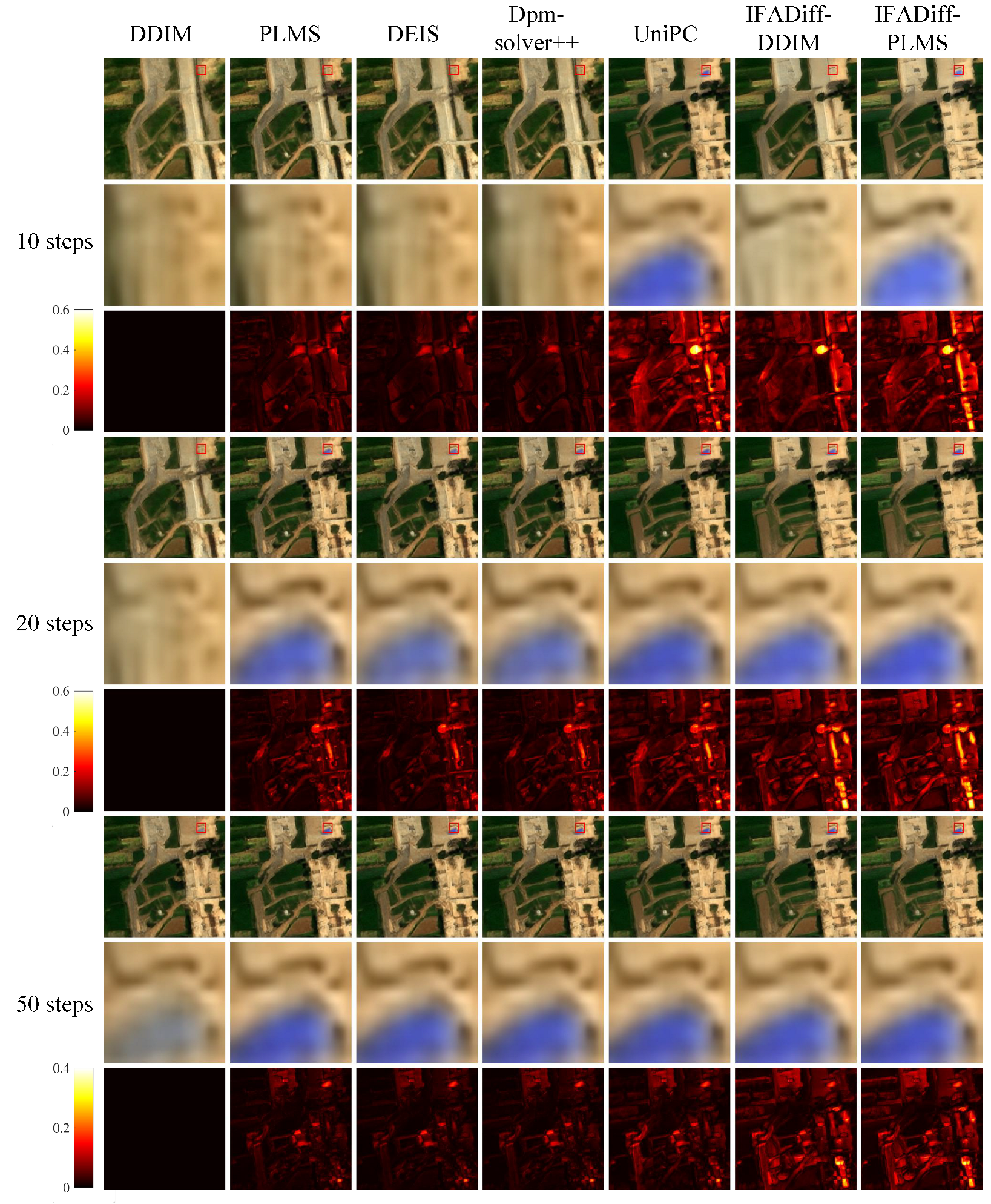
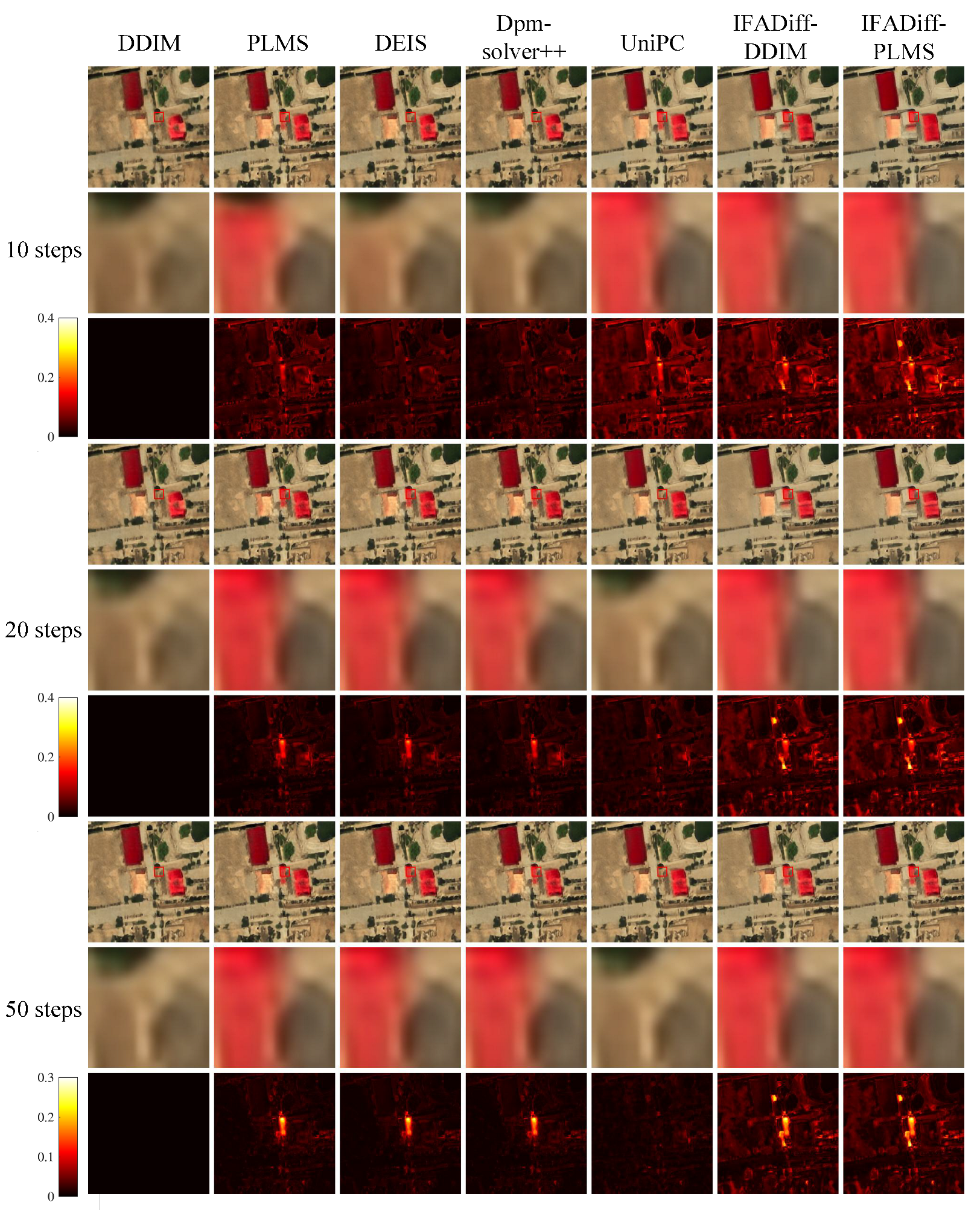
Visual comparisons further corroborate these findings. As shown in Figure 3, when the number of sampling steps is small, DDIM and PLMS often produce blurry textures and degraded spectral details. In contrast, IFADiff (DDIM) and IFADiff (PLMS), incorporating fractional-order corrections into the sampling process, generate sharper spatial structures and more consistent spectral characteristics. At 10 and 20 steps, IFADiff effectively reduces boundary artifacts and restores fine textures absent in the baselines. Although advanced solvers such as DPM-solver++ and UniPC also achieve competitive results with fewer steps, IFADiff exhibits superior stability, smoother convergence, and more balanced performance across visual and spectral metrics. Even with more sampling steps (e.g., 50), IFADiff continues to produce clearer edges and finer textures as results converge toward the baselines. These results demonstrate that the proposed alternating integer–fractional strategy not only accelerates convergence but also enhances spectral–spatial fidelity in high-dimensional HSI generation. Similar trends are observed in Appendix A.1.
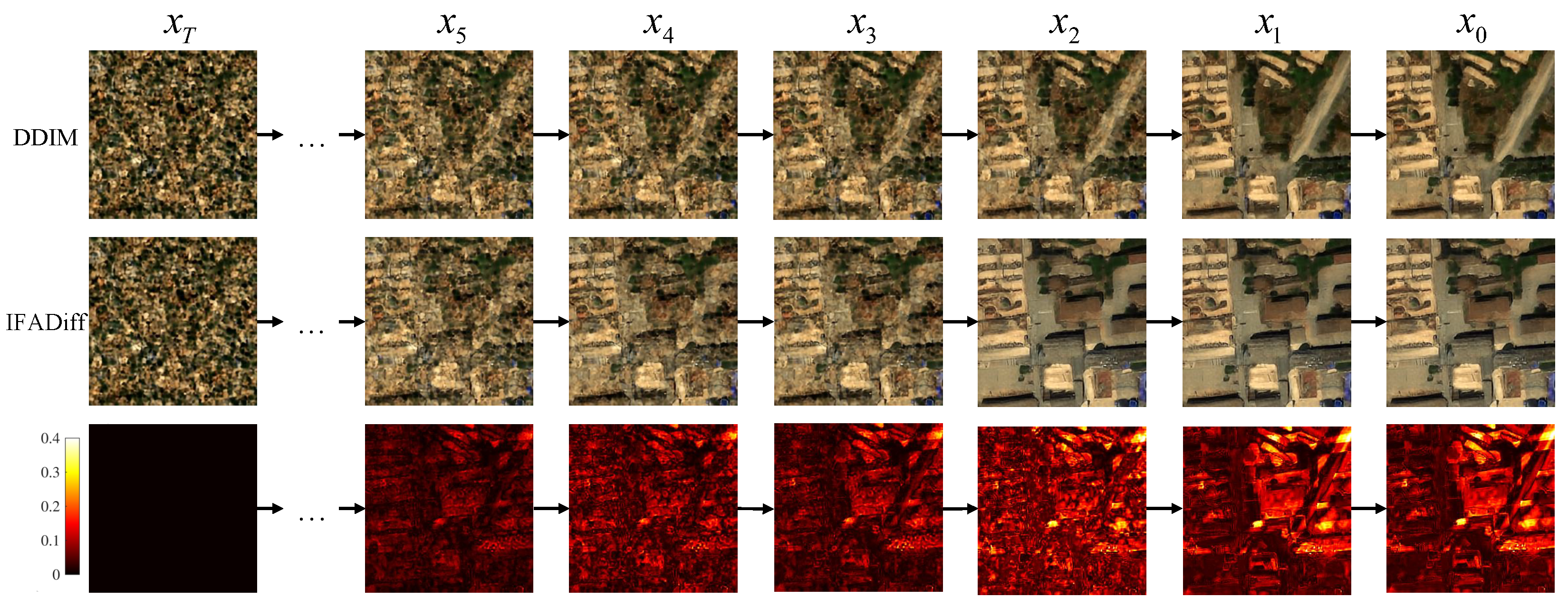
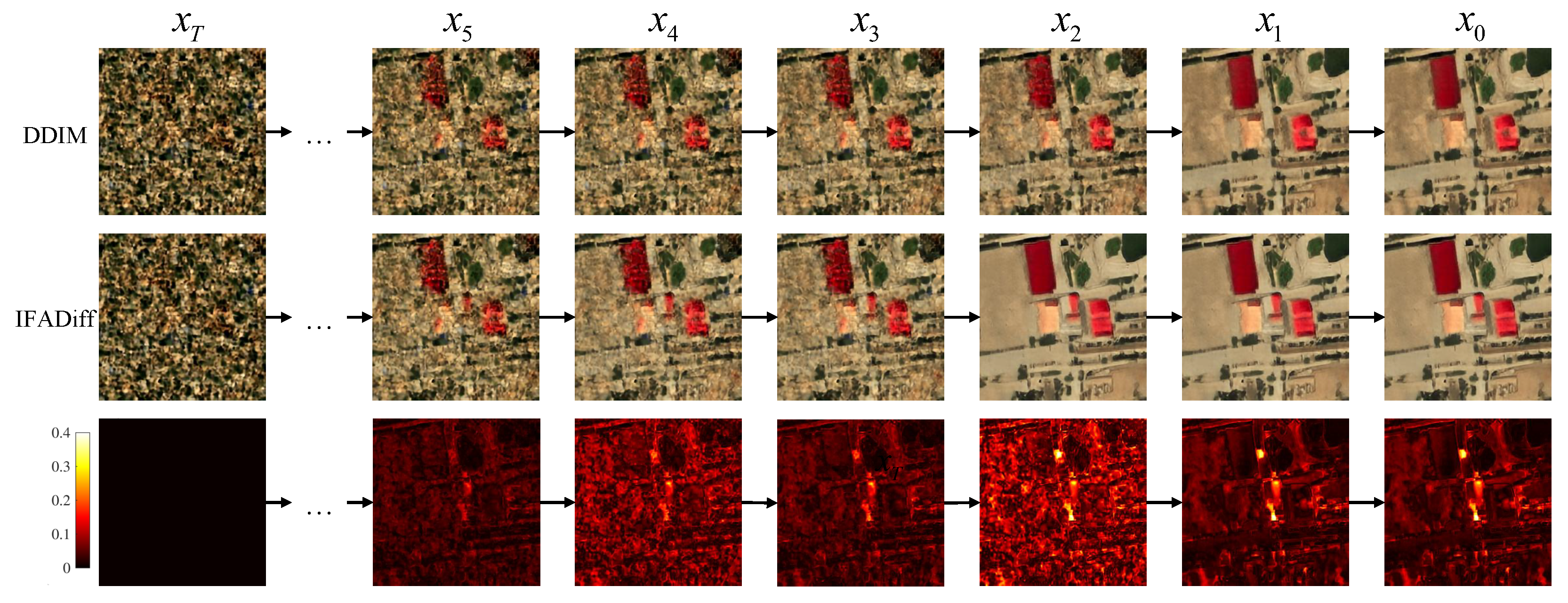
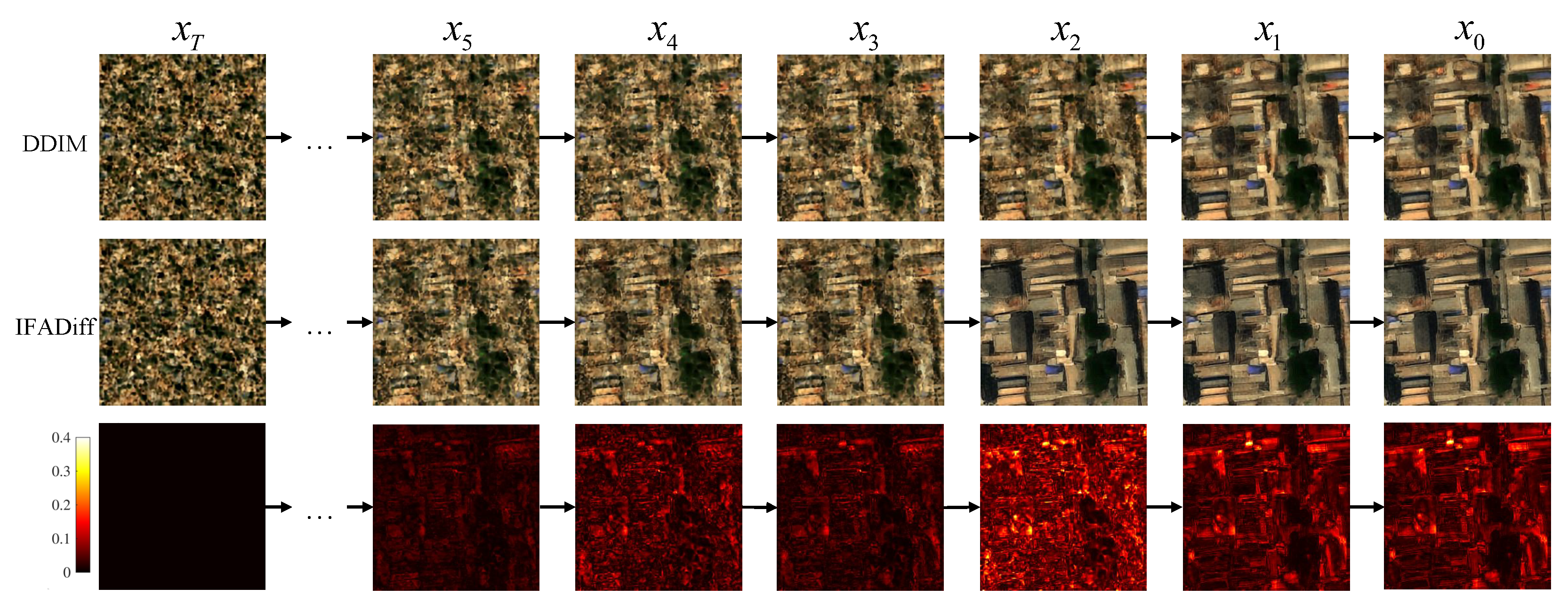
In addition, Figure 4 presents the intermediate denoising results of IFADiff and DDIM during the sampling process. It can be observed that IFADiff converges to the final result earlier and faster, showing stronger stability throughout the iterative process. Moreover, IFADiff demonstrates a superior ability to preserve emerging structural features in the intermediate stages, whereas DDIM tends to oversmooth or even erase these details in subsequent iterations.
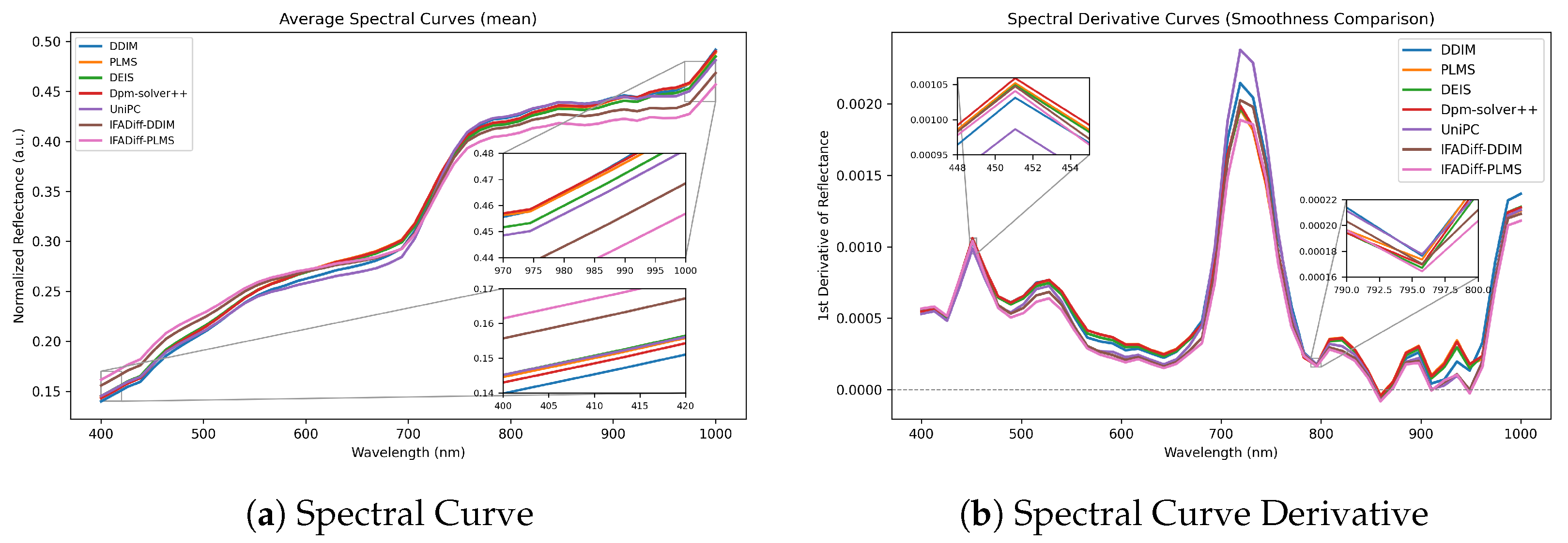
To assess the physical plausibility of the generated spectra, we analyze the average spectral reflectance and its first-order derivatives of the unconditionally generated HSIs. Since the employed model has no paired reference HSI for pixel-wise evaluation, we instead compare the average spectral curves of our method and the baselines. As shown in Figure 5, IFADiff produces smoother and more physically consistent spectral curves over 400–1000 nm. When combined with DDIM or PLMS, it suppresses high-frequency oscillations while preserving key reflectance transitions. The derivative plots also exhibit smaller fluctuation magnitudes than DPM-Solver++ and UniPC, indicating improved spectral smoothness and physical consistency.
We further evaluated the computational efficiency of IFADiff. As summarized in Table 3, IFADiff introduces negligible GPU memory and runtime overhead across different solvers and sampling steps. For instance, at 10 sampling steps, IFADiff ( α = 1.01 ) + DDIM requires only 0.7‰ additional memory and even slightly reduces inference time ( 1.36 % ) compared with DDIM. At higher steps (e.g., 50), all IFADiff variants maintain less than 1‰ memory overhead, while higher-order solvers such as DPM-solver++ and UniPC incur 5–10× greater resource costs. These results confirm that IFADiff significantly improves performance without sacrificing computational efficiency, making it practical for large-scale diffusion-based HSI generation.
Notably, we observe that the choice of fractional order α should vary with the number of sampling steps. When the step count is small and the baseline generation quality is relatively poor, a larger α is beneficial because it incorporates more information from past states, helping to compensate for insufficient predictions and improving spectral–spatial fidelity. However, as the number of steps increases, relying too heavily on historical states introduces redundant noise from earlier steps, making a smaller α preferable to avoid overcorrection and maintain stable, high-quality generation. In practice, α should be set relatively large for small step counts and gradually decreased as the steps grow, a trend consistently observed in both unconditional and conditional generation experiments.

5.3. Conditional Generation

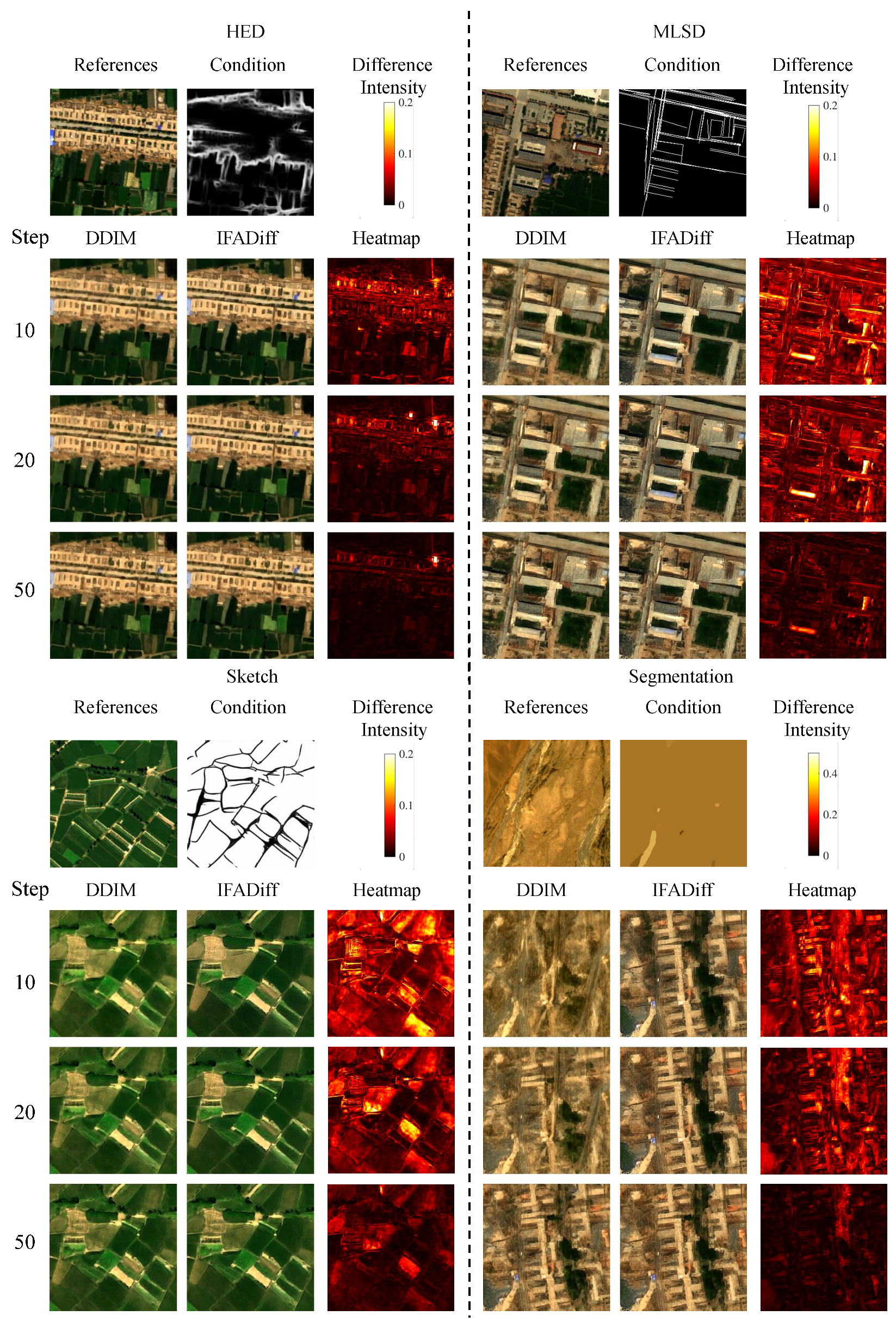
In the conditional generation experiments, we likewise employed the pretrained HSIGene model, using DDIM and PLMS under the uniform timestep setting as baseline solvers. Following CRSDiff [17], four types of conditional inputs were adopted to guide the generation process: HED (Holistically-nested Edge Detection), which extracts hierarchical edge and object boundary features; Segmentation, which provides semantic masks of the HSI data; Sketch, which represents the image as simplified line drawings capturing contours and structural shapes; and MLSD (Multiscale Line Segment Detection), which detects straight line segments to encode structural layouts. For each condition, we performed comparative analyses under 10, 20, and 50 sampling steps.
Table 4 reports the quantitative results for the HED condition. Across different step settings and α values, IFADiff consistently outperforms the DDIM baseline by achieving higher SSIM and NIMA scores, along with lower NIQE, BRISQUE, LPIPS, PIQE, RMSE, and SAM values. Similar to the unconditional generation setting, we also observe that larger α values are more suitable under fewer sampling steps, while α should be gradually reduced as the number of steps increases to avoid noise accumulation and overcorrection. These results indicate that IFADiff not only enhances the structural fidelity of the generated images but also improves their perceptual quality, especially under a small number of sampling steps. Similar trends are observed for the other conditional settings, confirming the general effectiveness of our method. The detailed quantitative comparisons for MLSD, Sketch, and Segmentation are provided in Appendix A.2.
Visual comparisons in Figure 6 further demonstrate these advantages. When guided by HED, MLSD, Sketch, or Segmentation maps, baseline DDIM often struggles to fully preserve structural cues, producing blurry or inconsistent textures under low sampling steps (e.g., 10). In contrast, IFADiff generates outputs that better align with the input conditions, recovering sharper boundaries in HED, more coherent line structures in MLSD and Sketch, and clearer region layouts in Segmentation. Notably, under HED, MLSD, and Segmentation conditions, the results obtained with only 10 steps are already close to those generated with 50 steps, further highlighting the efficiency of the proposed approach. Even at larger step counts (20 or 50), IFADiff continues to deliver improvements, underscoring the benefits of the integer–fractional alternating inference strategy for conditional HSI generation.

5.4. Ablation Study

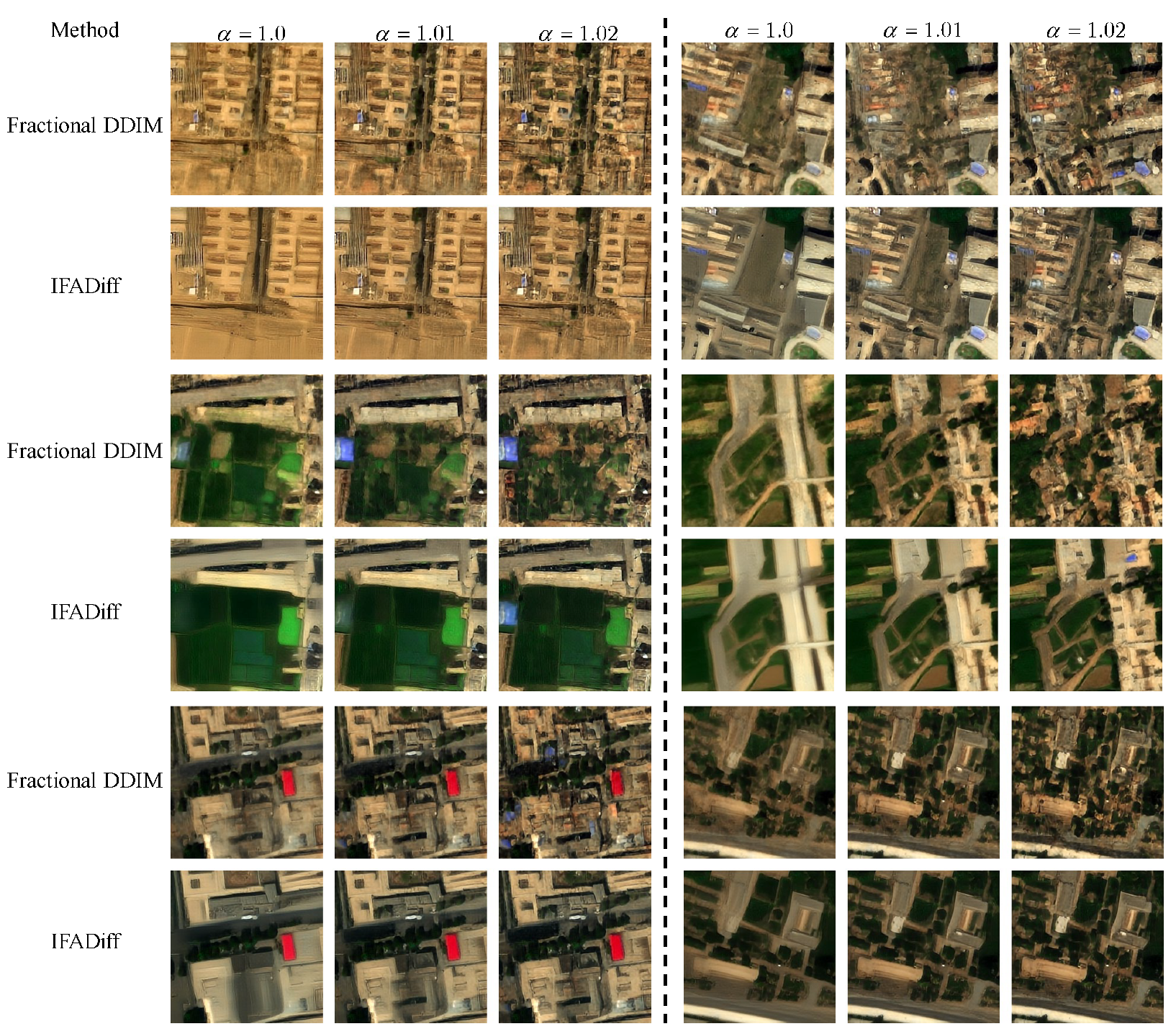
In this section, we analyze the effect of the fractional order α on the performance of IFADiff. The experiments were conducted under the unconditional generation setting with 10 sampling steps. The results for 20 and 50 sampling steps are provided in Appendix A.3, and they lead to conclusions consistent with those observed under 10 steps. We compared the proposed IFADiff, which alternates between integer-order and fractional-order updates, against two counterparts: the standard integer-order DDIM and the purely fractional-order variant (denoted as Fractional DDIM). Notably, when α = 1 , Fractional DDIM reduces to the standard DDIM solver, serving as a natural reference point for comparison. Such a three-way comparison highlights the respective strengths and weaknesses of integer-only and fractional-only approaches, and more clearly demonstrates the advantages of the alternating strategy in achieving stable and high-quality HSI generation.
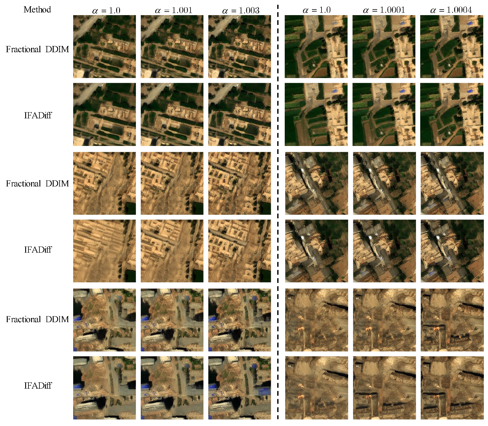
As shown in Table 5 and Figure 7, when α = 1.0 , IFADiff achieves the highest IS score, but its PIQE value does not surpass that of DDIM and the outputs appear overly smoothed with suppressed details. This inconsistency arises from the nature of IS: since it measures classifier confidence, smoother images with reduced high-frequency noise yield sharper posterior distributions, thereby inflating the score. However, this does not imply better perceptual quality—BRISQUE and PIQE clearly indicate that oversmoothing degrades naturalness and fidelity, underscoring the need for multiple metrics beyond IS. Because results at α = 1.0 already suffer from excessive smoothness, we did not test smaller values, as they would exacerbate this issue. Therefore, our experiments focus on α > 1.0 . As α increases toward 1.02, IFADiff achieves the best BRISQUE and PIQE while maintaining competitive IS, and the generated images exhibit richer textures and greater diversity. However, when α exceeds 1.02, the generation process becomes prone to instability and amplified noise, leading to a degradation in overall image quality, with IS scores even falling below those of DDIM.
Therefore, in practical applications, α can be flexibly adjusted according to user requirements: values closer to 1.0 (e.g., around 1.01) are preferable when smoother and cleaner outputs with fewer artifacts are desired, whereas slightly larger values (e.g., around 1.02) are suitable for scenarios prioritizing richer details and higher content diversity. Consequently, the optimal range of α lies between 1.01 and 1.02. This trade-off is consistent with the trends observed in the conditional generation experiments, where smaller α values favor structural clarity under sufficient sampling steps, while larger values better preserve fine-grained details when fewer steps are available.
6. Discussion

6.1. Experimental Discussion

The experimental results in both unconditional and conditional settings confirm the effectiveness of IFADiff for hyperspectral image (HSI) generation. Compared with integer-order solvers, IFADiff consistently yields higher spectral–spatial fidelity, sharper textures, and faster convergence under various sampling budgets. These gains arise from its alternating design, which combines the stability of integer-order prediction with the global consistency of fractional-order correction, and from its fully training-free, plug-and-play nature that allows seamless integration into existing diffusion solvers.
A key finding is that the fractional order parameter α controls the trade-off between fine-grained detail and global smoothness: larger α is preferable for small sampling budgets, while smaller α improves stability at larger step counts. In our experiments, we set α close to but slightly larger than 1 in a step-dependent manner (e.g., α [ 1.01 , 1.02 ] for 10 steps, α [ 1.001 , 1.003 ] for 20 steps, and α [ 1.0001 , 1.0004 ] for 50 steps), which yields a practical balance of convergence, smoothness, and detail.
Since an overly large α may cause overshooting, we also consider simple schedules that use a slightly larger α in the early steps and gradually decrease it in later steps. In future work, we plan to make this more principled by adapting α during sampling according to local spectral variance or gradient magnitude. As a preliminary verification, Table 6 compares fixed fractional orders with such linear schedules (e.g., 1.01 to 0.99 denotes a linear decay of α from 1.01 to 0.99 along the diffusion timesteps), showing that adaptive variants generally improve IS, BRISQUE, PIQE, RMSE, and SAM across different sampling steps, while the NIMA score is only slightly lower than the best fixed- α configuration, suggesting that content-aware adaptive designs are a promising direction for future research.
Despite its strengths, IFADiff still has several limitations. The fractional correction step introduces a small computational overhead compared with pure integer-order solvers, so optimizing the weighting scheme and exploring hardware-friendly implementations will be important for real-time deployment. In addition, although our experiments consider multiple random seeds and test settings, further evaluation on larger-scale real-world hyperspectral datasets is needed to more fully assess robustness and generalization.

6.2. Limitations and Future Work

Under complex atmospheric and illumination conditions (e.g., haze, cloud cover, humidity changes, low light), IFADiff usually provides more stable reconstructions and better detail preservation than integer-order solvers, as its fractional memory helps retain global structure and spectral smoothness. However, when early states are heavily contaminated by noise or atmospheric distortions, the aggregation of historical information can also propagate errors, causing local spectral bias or spatial artifacts. In such cases, a single global fractional order or fixed truncation length may be suboptimal: larger orders risk amplifying noise, whereas smaller orders weaken the benefits of long-range memory.
To address these challenges, future extensions of IFADiff could integrate adaptive fractional mechanisms and physics-informed constraints. Dynamically adjusting the fractional order and truncation length according to local signal-to-noise ratios or atmospheric transmittance, combined with illumination-aware weighting, robust aggregation, and frequency-domain smoothing, may improve spectral stability and generalization under challenging real-world atmospheric, noisy, and low-light conditions.
Beyond hyperspectral image generation, IFADiff also has potential for broader applications. As diffusion models are increasingly used in natural image synthesis, medical imaging, and scientific data modeling, a training-free framework that improves inference quality without modifying model weights is of practical value. The alternating integer–fractional formulation offers a general mechanism for iterative error correction and stability enhancement, which could inspire new diffusion solvers for high-dimensional or data-scarce settings and promote more theoretically grounded, memory-aware sampling algorithms.

7. Conclusions

In this paper, we presented IFADiff, a training-free inference framework for hyperspectral image generation that alternates integer-order prediction with fractional-order correction. Starting from standard ODE-based samplers such as DDIM and PLMS, IFADiff augments each update with a truncated Grünwald–Letnikov fractional combination of historical states, enabling long-range dependency modeling while preserving the stability and efficiency of integer-order solvers. This integer–fractional alternating design can be interpreted as a general predictor–corrector mechanism, in which integer steps provide fast provisional updates and fractional steps refine spectral consistency and spatial detail through memory-aware aggregation, and can in principle be applied to a broad family of integer-order diffusion samplers.
Extensive experiments on unconditional and conditional HSI synthesis demonstrate that IFADiff consistently improves both reference-based and no-reference image quality metrics across different sampling budgets and solver backbones. Visual comparisons further show reduced spectral drift, sharper textures, and clearer structures compared with purely integer-order or purely fractional-order methods. Moreover, the fractional order α acts as an interpretable control parameter that balances texture richness and smoothness, offering flexible quality–efficiency trade-offs without any retraining or architectural changes. Overall, IFADiff provides an efficient, general, and easily deployable enhancement module for high-quality hyperspectral diffusion sampling.

Author Contributions

Conceptualization, Y.Y., X.J., W.W., W.S., H.Z. and Z.J.; Methodology, Y.Y. and X.J.; Software, Y.Y.; Validation, Y.Y.; Formal analysis, Y.Y., X.J., W.W., W.S., H.Z. and Z.J. Investigation, Y.Y., W.W., W.S., H.Z. and Z.J. Resources, Y.Y.; Data curation, Y.Y.; Writing—original draft, Y.Y.; Writing—review & editing, Y.Y. and X.J.; Visualization, Y.Y.; Supervision, X.J., W.W. and W.S.; Project administration, X.J., W.W., W.S., H.Z. and Z.J.; Funding acquisition, X.J. All authors have read and agreed to the published version of the manuscript.

Funding

This research was funded by the National Natural Science Foundation of China (Grants Nos.62372359, 61772389, 61972264) and the Xidian University Specially Funded Project for Interdisciplinary Exploration (TZJHF202513).

Data Availability Statement

We have revised the Data Availability Statement as follows: The original data presented in the study are openly available from the following repositories: The Xiongan Dataset from the Chinese Academy of Sciences (CAS) (https://aistudio.baidu.com/datasetdetail/283692, accessed on 17 November 2025); The DFC2013 Dataset from the University of Houston, Cullen College of Engineering, Department of Electrical & Computer Engineering (https://machinelearning.ee.uh.edu/2013-ieee-grss-data-fusion-contest/, accessed on 17 November 2025); The DFC2018 Dataset from the University of Houston, Cullen College of Engineering, Department of Electrical & Computer Engineering (https://machinelearning.ee.uh.edu/2018-ieee-grss-data-fusion-challenge-fusion-of-multispectral-lidar-and-hyperspectral-data/, accessed on 17 November 2025); The HiWATER Dataset from the National Tibetan Plateau Data Center (TPDC) (https://doi.org/10.3972/hiwater.011.2013.db, accessed on 17 November 2025); The AID Dataset from Hugging Face Datasets (https://huggingface.co/datasets/blanchon/AID, accessed on 17 November 2025).

Acknowledgments

The authors would like to thank the editors and the anonymous reviewers for their constructive comments and suggestions.

Conflicts of Interest

The authors declare no conflict of interest.

Appendix A. Supplementary Experiments

Appendix A.1. Unconditional Generation

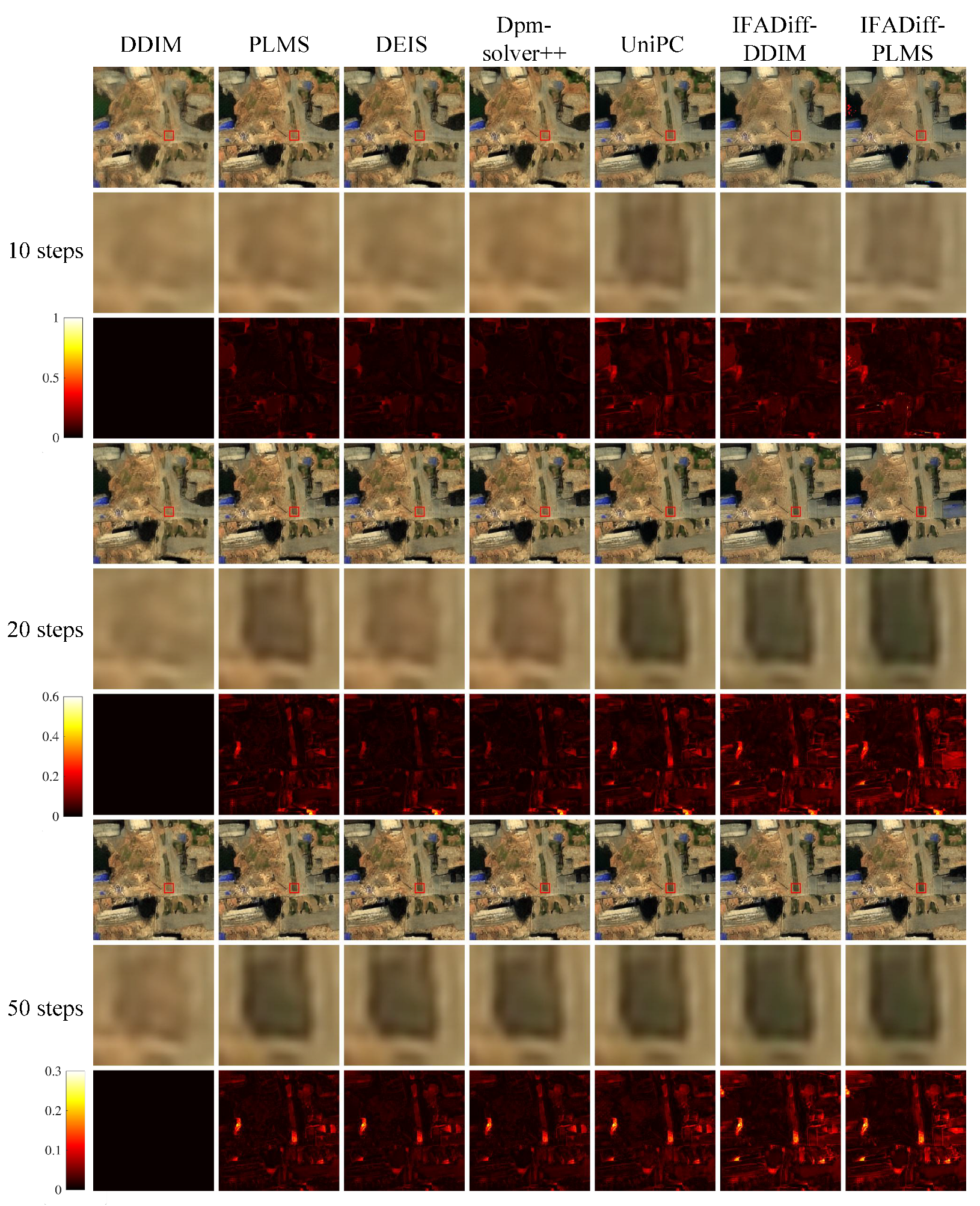
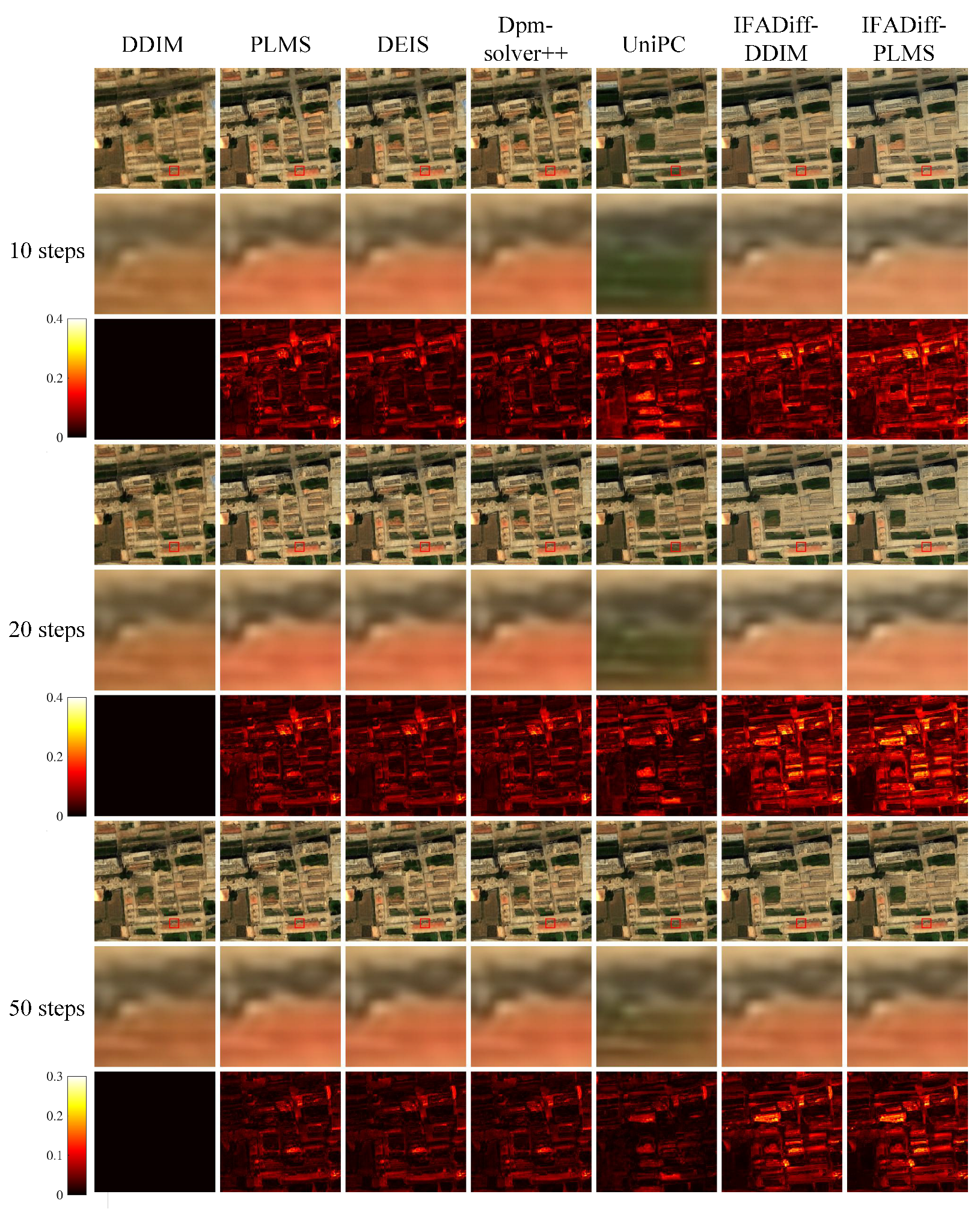
In addition to the quantitative comparisons presented in the main text, we provide supplementary visual results for unconditional HSI generation. Figure A1 and Figure A2 show intermediate reconstructions and corresponding heatmaps for DDIM and IFADiff-DDIM at 20 steps, revealing how the fractional correction step refines spatial–spectral structures and suppresses artifacts during sampling.
Figure A3, Figure A4 and Figure A5 show full unconditional generation results at 10, 20, and 50 sampling steps using DDIM and PLMS with and without IFADiff under three random seeds. Across all seeds and step counts, IFADiff yields clearer structures, sharper edges, and more reliable spectral details, and maintains higher spatial–spectral coherence even at larger step numbers. Together with the intermediate reconstructions in Figure A1 and Figure A2, these results confirm that the alternating integer–fractional strategy improves the stability and quality of unconditional generation under diverse sampling settings.
Figure A1. Intermediate results and heatmaps for unconditional generation (second random seed).
Remotesensing 17 03867 g0a1
Figure A2. Intermediate results and heatmaps for unconditional generation (third random seed).
Remotesensing 17 03867 g0a2

Appendix A.2. Conditional Generation

To supplement the main text, this appendix provides the detailed quantitative comparisons for the remaining three types of conditional inputs: MLSD, Sketch, and Segmentation. For each condition, we evaluate the generation quality at 10, 20, and 50 sampling steps. Baseline solvers (DDIM) are compared directly with their corresponding IFADiff-enhanced versions, following the same uniform timestep setting as in the main experiments.
Consistent with the HED results in Table 4, the additional results in Table A1 (MLSD), Table A2 (Sketch), and Table A3 (Segmentation) show that IFADiff consistently outperforms the baseline across all conditions and step counts. This confirms that IFADiff improves both structural fidelity and perceptual quality in conditional generation, demonstrating robust and general behavior under diverse guidance settings.

Appendix A.3. Ablation Study

To complement the ablation results reported in the main text for 10 sampling steps, this appendix provides the corresponding quantitative and visual comparisons for 20 and 50 steps. We evaluate three variants: the standard integer-order solver (DDIM), the purely fractional-order solver (Fractional DDIM), and the proposed alternating strategy (IFADiff with DDIM). As in the 10-step setting, the results in Table A4 show that IFADiff achieves superior spectral–spatial fidelity compared with both integer-only and fractional-only solvers. Specifically, IFADiff yields higher IS and NIMA scores and lower BRISQUE and PIQE values across different fractional orders α , while maintaining more stable quality than Fractional DDIM, which is highly sensitive to α and prone to artifacts.
The additional results for 20 and 50 steps, illustrated in Figure A6, further confirm the robustness of IFADiff. Although DDIM improves with more steps, residual blur and weak textures remain compared with IFADiff. When α = 1.0 , IFADiff also generates overly smoothed outputs, highlighting the need for slightly larger α values to recover richer textures. In contrast, Fractional DDIM remains unstable across different α , while IFADiff consistently produces clearer structures, more reliable spectral details, and better quantitative scores than both counterparts. For 20 steps, moderately larger values (around 1.001–1.003) strike a good balance, while for 50 steps, smaller values (around 1.0001–1.0004) are preferable. Overall, larger α emphasizes richer details, whereas smaller α yields smoother and cleaner outputs, offering flexibility for different application needs.
Figure A3. Supplementary unconditional generation results (second random seed).
Remotesensing 17 03867 g0a3
Figure A4. Supplementary unconditional generation results (third random seed).
Remotesensing 17 03867 g0a4
Figure A5. Supplementary unconditional generation results (fourth random seed).
Remotesensing 17 03867 g0a5
Table A1. Quantitative results of conditional HSI generation with the MLSD condition at 10, 20, and 50 sampling steps.
StepMethodSSIM ↑NIQE ↓BRISQUE ↓LPIPS ↓PIQE ↓NIMA ↑RMSE ↓SAM ↓
10DDIM0.118 ± 0.0155.829 ± 0.70730.598 ± 4.6690.536 ± 0.01948.941 ± 10.1643.677 ± 0.1050.090 ± 0.0150.150 ± 0.020
IFADiff ( α = 1.015 )0.112 ± 0.0185.724 ± 0.38822.017 ± 3.8430.533 ± 0.02242.530 ± 9.3883.858 ± 0.1290.083 ± 0.0160.144 ± 0.020
20DDIM0.116 ± 0.0195.663 ± 0.64228.038 ± 4.4290.531 ± 0.02045.836 ± 9.7943.675 ± 0.1050.088 ± 0.0150.148 ± 0.019
IFADiff ( α = 1.002 )0.118 ± 0.0245.642 ± 0.44822.307 ± 4.4300.528 ± 0.02341.793 ± 8.9363.851 ± 0.1220.082 ± 0.0160.143 ± 0.018
50DDIM0.112 ± 0.0215.565 ± 0.60526.816 ± 4.2050.528 ± 0.01943.124 ± 9.1213.663 ± 0.0980.086 ± 0.0150.147 ± 0.018
IFADiff ( α = 1.0001 )0.118 ± 0.0245.557 ± 0.49724.759 ± 4.5670.522 ± 0.02141.303 ± 8.7523.758 ± 0.1060.080 ± 0.0160.142 ± 0.018
Table A2. Quantitative results of conditional HSI generation with the Sketch condition at 10, 20, and 50 sampling steps.
StepMethodSSIM ↑NIQE ↓BRISQUE ↓LPIPS ↓PIQE ↓NIMA ↑RMSE ↓SAM ↓
10DDIM0.162 ± 0.0165.873 ± 0.79031.169 ± 4.5130.489 ± 0.02045.129 ± 9.1223.712 ± 0.0870.089 ± 0.0150.149 ± 0.020
IFADiff ( α = 1.015 )0.156 ± 0.0215.707 ± 0.32422.807 ± 4.2260.485 ± 0.02539.482 ± 8.7363.869 ± 0.0960.082 ± 0.0160.143 ± 0.019
20DDIM0.161 ± 0.0205.696 ± 0.60629.251 ± 4.5790.482 ± 0.01942.648 ± 8.5863.704 ± 0.0780.087 ± 0.0150.147 ± 0.019
IFADiff ( α = 1.002 )0.164 ± 0.0275.598 ± 0.39523.545 ± 4.6110.483 ± 0.02538.975 ± 8.1453.870 ± 0.0890.080 ± 0.0160.142 ± 0.018
50DDIM0.156 ± 0.0235.555 ± 0.51928.158 ± 4.3720.479 ± 0.01840.408 ± 8.1783.685 ± 0.0730.085 ± 0.0140.146 ± 0.018
IFADiff ( α = 1.0001 )0.163 ± 0.0275.525 ± 0.32726.069 ± 4.5950.477 ± 0.02138.825 ± 7.9283.772 ± 0.0770.079 ± 0.0150.141 ± 0.017
Table A3. Quantitative results of conditional HSI generation with the Segmentation condition at 10, 20, and 50 sampling steps.
StepMethodSSIM ↑NIQE ↓BRISQUE ↓LPIPS ↓PIQE ↓NIMA ↑RMSE ↓SAM ↓
10DDIM0.325 ± 0.0165.747 ± 0.52230.680 ± 5.2060.409 ± 0.01445.178 ± 7.8403.745 ± 0.0670.088 ± 0.0150.148 ± 0.020
IFADiff ( α = 1.015 )0.320 ± 0.0275.642 ± 0.44323.464 ± 4.1950.405 ± 0.01741.142 ± 7.1993.868 ± 0.0530.081 ± 0.0160.142 ± 0.019
20DDIM0.314 ± 0.0205.621 ± 0.47128.873 ± 5.4520.407 ± 0.01242.627 ± 7.7053.738 ± 0.0660.086 ± 0.0150.147 ± 0.019
IFADiff ( α = 1.002 )0.317 ± 0.0305.542 ± 0.51324.059 ± 4.4380.402 ± 0.01940.344 ± 7.0853.856 ± 0.0690.080 ± 0.0160.141 ± 0.018
50DDIM0.302 ± 0.0235.549 ± 0.46028.039 ± 5.1150.408 ± 0.01040.091 ± 7.2863.722 ± 0.0660.084 ± 0.0140.145 ± 0.018
IFADiff ( α = 1.0001 )0.309 ± 0.0275.468 ± 0.45326.176 ± 5.1090.401 ± 0.01439.521 ± 7.1713.781 ± 0.0770.078 ± 0.0150.140 ± 0.017
Table A4. Ablation study results of unconditional HSI generation under 20 and 50 sampling steps. Performance metrics are reported for different fractional orders α using Fractional DDIM and IFADiff.
StepMethod α TypeIS ↑BRISQUE ↓PIQE ↓NIMA ↑RMSE ↓SAM ↓
20DDIM1.0Int.3.68 ± 0.0227.068 ± 0.18741.063 ± 0.1563.748 ± 0.0090.092 ± 0.0180.154 ± 0.026
IFADiffInt.4.21 ± 0.0623.304 ± 0.15040.998 ± 0.2583.936 ± 0.0050.084 ± 0.0180.149 ± 0.025
Frac. DDIM1.001Frac.3.49 ± 0.0726.202 ± 0.15840.181 ± 0.2563.724 ± 0.0030.094 ± 0.0190.156 ± 0.027
IFADiffInt. + Frac.4.13 ± 0.0222.768 ± 0.20638.69 ± 0.1683.909 ± 0.0070.080 ± 0.0270.145 ± 0.039
Frac. DDIM1.003Frac.3.63 ± 0.0725.179 ± 0.16738.435 ± 0.2333.702 ± 0.0040.097 ± 0.0200.159 ± 0.029
IFADiffInt. + Frac.3.70 ± 0.0521.806 ± 0.25935.845 ± 0.1893.856 ± 0.0050.082 ± 0.0280.147 ± 0.040
50DDIM1.0Int.3.69 ± 0.0525.993 ± 0.24138.807 ± 0.1403.732 ± 0.0100.088 ± 0.0180.156 ± 0.027
IFADiffInt.3.85 ± 0.0324.101 ± 0.11738.177 ± 0.2343.799 ± 0.0060.081 ± 0.0170.151 ± 0.025
Frac. DDIM1.0001Frac.3.59 ± 0.0625.630 ± 0.21538.778 ± 0.1083.720 ± 0.0050.090 ± 0.0180.158 ± 0.027
IFADiffInt. + Frac.3.80 ± 0.0323.912 ± 0.25637.371 ± 0.2183.801 ± 0.0090.078 ± 0.0220.147 ± 0.033
Frac. DDIM1.0004Frac.3.63 ± 0.0825.222 ± 0.26137.957 ± 0.2253.716 ± 0.0090.091 ± 0.0190.159 ± 0.028
IFADiffInt. + Frac.3.72 ± 0.0423.489 ± 0.13136.335 ± 0.1433.780 ± 0.0060.079 ± 0.0230.148 ± 0.033
Figure A6. Unconditional HSI generation results under 20 (left) and 50 (right) sampling steps. Across both settings, IFADiff consistently improves spectral–spatial fidelity over integer-only and fractional-only baselines, demonstrating robustness across different sampling budgets and random seeds.
Remotesensing 17 03867 g0a6

References

  1. Pang, L.; Rui, X.; Cui, L.; Wang, H.; Meng, D.; Cao, X. HIR-Diff: Unsupervised Hyperspectral Image Restoration Via Improved Diffusion Models. In Proceedings of the IEEE/CVF Conference on Computer Vision and Pattern Recognition, Seattle, WA, USA, 17–21 June 2024; pp. 3005–3014. [Google Scholar]
  2. Li, M.; Liu, J.; Fu, Y.; Zhang, Y.; Dou, D. Spectral enhanced rectangle transformer for hyperspectral image denoising. In Proceedings of the IEEE/CVF Conference on Computer Vision and Pattern Recognition, Vancouver, BC, Canada, 14–24 June 2023; pp. 5805–5814. [Google Scholar]
  3. Wang, X.; Hu, Q.; Cheng, Y.; Ma, J. Hyperspectral image super-resolution meets deep learning: A survey and perspective. IEEE/CAA J. Autom. Sin. 2023, 10, 1668–1691. [Google Scholar] [CrossRef]
  4. Ahmad, M.; Distefano, S.; Khan, A.M.; Mazzara, M.; Li, C.; Li, H.; Aryal, J.; Ding, Y.; Vivone, G.; Hong, D. A comprehensive survey for hyperspectral image classification: The evolution from conventional to transformers and mamba models. Neurocomputing 2025, 644, 130428. [Google Scholar] [CrossRef]
  5. Xue, J.; Zhao, Y.Q.; Wu, T.; Chan, J.C.W. Tensor convolution-like low-rank dictionary for high-dimensional image representation. IEEE Trans. Circuits Syst. Video Technol. 2024, 34, 13257–13270. [Google Scholar] [CrossRef]
  6. Goodfellow, I.; Pouget-Abadie, J.; Mirza, M.; Xu, B.; Warde-Farley, D.; Ozair, S.; Courville, A.; Bengio, Y. Generative adversarial nets. Adv. Neural Inf. Process. Syst. 2014, 27, 2672–2680. [Google Scholar]
  7. Kingma, D.P.; Welling, M. Auto-encoding variational bayes. arXiv 2013, arXiv:1312.6114. [Google Scholar]
  8. Ho, J.; Jain, A.; Abbeel, P. Denoising diffusion probabilistic models. Adv. Neural Inf. Process. Syst. 2020, 33, 6840–6851. [Google Scholar]
  9. Dhariwal, P.; Nichol, A. Diffusion models beat gans on image synthesis. Adv. Neural Inf. Process. Syst. 2021, 34, 8780–8794. [Google Scholar]
  10. Rombach, R.; Blattmann, A.; Lorenz, D.; Esser, P.; Ommer, B. High-resolution image synthesis with latent diffusion models. In Proceedings of the IEEE/CVF Conference on Computer Vision and Pattern Recognition, New Orleans, LA, USA, 18–24 June 2022; pp. 10684–10695. [Google Scholar]
  11. Yu, Y.; Pan, E.; Wang, X.; Wu, Y.; Mei, X.; Ma, J. Unmixing Before Fusion: A Generalized Paradigm for Multi-Source-based Hyperspectral Image Synthesis. In Proceedings of the IEEE/CVF Conference on Computer Vision and Pattern Recognition, Seattle, WA, USA, 16–22 June 2024; pp. 9297–9306. [Google Scholar]
  12. Yu, Y.; Pan, E.; Ma, Y.; Mei, X.; Chen, Q.; Ma, J. UnmixDiff: Unmixing-based Diffusion Model for Hyperspectral Image Synthesis. IEEE Trans. Geosci. Remote Sens. 2024, 62, 5524018. [Google Scholar] [CrossRef]
  13. Pang, L.; Cao, X.; Tang, D.; Xu, S.; Bai, X.; Zhou, F.; Meng, D. Hsigene: A foundation model for hyperspectral image generation. arXiv 2024, arXiv:2409.12470. [Google Scholar] [CrossRef]
  14. Zhang, L.; Rao, A.; Agrawala, M. Adding conditional control to text-to-image diffusion models. In Proceedings of the IEEE/CVF International Conference on Computer Vision, Paris, France, 2–6 October 2023; pp. 3836–3847. [Google Scholar]
  15. Song, J.; Meng, C.; Ermon, S. Denoising diffusion implicit models. arXiv 2020, arXiv:2010.02502. [Google Scholar]
  16. Chen, C.; Wang, Y.; Zhang, N.; Zhang, Y.; Zhao, Z. A review of hyperspectral image super-resolution based on deep learning. Remote Sens. 2023, 15, 2853. [Google Scholar] [CrossRef]
  17. Tang, D.; Cao, X.; Hou, X.; Jiang, Z.; Meng, D. Crs-diff: Controllable generative remote sensing foundation model. arXiv 2024, arXiv:2403.11614. [Google Scholar] [CrossRef]
  18. Sebaq, A.; ElHelw, M. Rsdiff: Remote sensing image generation from text using diffusion model. Neural Comput. Appl. 2024, 36, 23103–23111. [Google Scholar] [CrossRef]
  19. Khanna, S.; Liu, P.; Zhou, L.; Meng, C.; Rombach, R.; Burke, M.; Lobell, D.B.; Ermon, S. Diffusionsat: A generative foundation model for satellite imagery. In Proceedings of the The Twelfth International Conference on Learning Representations, Kigali, Rwanda, 1–5 May 2023. [Google Scholar]
  20. Liu, L.; Ren, Y.; Lin, Z.; Zhao, Z. Pseudo numerical methods for diffusion models on manifolds. arXiv 2022, arXiv:2202.09778. [Google Scholar] [CrossRef]
  21. Zhang, Q.; Chen, Y. Fast sampling of diffusion models with exponential integrator. arXiv 2022, arXiv:2204.13902. [Google Scholar]
  22. Lu, C.; Zhou, Y.; Bao, F.; Chen, J.; Li, C.; Zhu, J. Dpm-solver: A fast ode solver for diffusion probabilistic model sampling in around 10 steps. Adv. Neural Inf. Process. Syst. 2022, 35, 5775–5787. [Google Scholar]
  23. Zhao, W.; Bai, L.; Rao, Y.; Zhou, J.; Lu, J. Unipc: A unified predictor-corrector framework for fast sampling of diffusion models. Adv. Neural Inf. Process. Syst. 2023, 36, 49842–49869. [Google Scholar]
  24. Song, Y.; Sohl-Dickstein, J.; Kingma, D.P.; Kumar, A.; Ermon, S.; Poole, B. Score-based generative modeling through stochastic differential equations. arXiv 2020, arXiv:2011.13456. [Google Scholar]
  25. Dormand, J.R.; Prince, P.J. A family of embedded Runge-Kutta formulae. J. Comput. Appl. Math. 1980, 6, 19–26. [Google Scholar] [CrossRef]
  26. Grathwohl, W.; Chen, R.T.; Bettencourt, J.; Sutskever, I.; Duvenaud, D. Ffjord: Free-form continuous dynamics for scalable reversible generative models. arXiv 2018, arXiv:1810.01367. [Google Scholar] [CrossRef]
  27. Sauer, T. Numerical Analysis; Pearson: London, UK, 2018. [Google Scholar]
  28. Oldham, K.; Spanier, J. The Fractional Calculus Theory and Applications of Differentiation and Integration to Arbitrary Order; Elsevier: Amsterdam, The Netherlands, 1974; Volume 111. [Google Scholar]
  29. Miller, K.S.; Ross, B. An Introduction to the Fractional Calculus and Fractional Differential Equations; John Wiley & Sons: New York, NY, USA, 1993. [Google Scholar]
  30. Tian, W.; Zhou, H.; Deng, W. A class of second order difference approximations for solving space fractional diffusion equations. Math. Comput. 2015, 84, 1703–1727. [Google Scholar] [CrossRef]
  31. Zhou, H.; Tian, W.; Deng, W. Quasi-compact finite difference schemes for space fractional diffusion equations. J. Sci. Comput. 2013, 56, 45–66. [Google Scholar] [CrossRef]
  32. Hao, Z.p.; Sun, Z.z.; Cao, W.r. A fourth-order approximation of fractional derivatives with its applications. J. Comput. Phys. 2015, 281, 787–805. [Google Scholar] [CrossRef]
  33. Lu, C.; Zhou, Y.; Bao, F.; Chen, J.; Li, C.; Zhu, J. Dpm-solver++: Fast solver for guided sampling of diffusion probabilistic models. Mach. Intell. Res. 2025, 22, 730–751. [Google Scholar] [CrossRef]
  34. Yi, C.; Zhang, L.; Zhang, X.; Yueming, W.; Wenchao, Q.; Senlin, T.; Zhang, P. Aerial hyperspectral remote sensing classification dataset of Xiongan New Area (Matiwan Village). Natl. Remote Sens. Bull. 2020, 24, 1299–1306. [Google Scholar]
  35. Yokoya, N.; Iwasaki, A. Airborne Hyperspectral Data over Chikusei; Technical Report SAL-2016-05-27; Space Application Laboratory, University of Tokyo: Bunkyō, Japan, 2016. [Google Scholar]
  36. Wen, J.; Xiao, Q. HiWATER: Visible and Near-Infrared Hyperspectral Radiometer (7 July 2012). 2013. Available online: https://doi.org/10.3972/hiwater.011.2013.db (accessed on 17 November 2025).
  37. Li, X.; Liu, S.; Xiao, Q.; Ma, M.; Jin, R.; Che, T.; Wang, W.; Hu, X.; Xu, Z.; Wen, J.; et al. A multiscale dataset for understanding complex eco-hydrological processes in a heterogeneous oasis system. Sci. Data 2017, 4, 170083. [Google Scholar] [CrossRef]
  38. Liu, L.; Li, W.; Shi, Z.; Zou, Z. Physics-informed hyperspectral remote sensing image synthesis with deep conditional generative adversarial networks. IEEE Trans. Geosci. Remote Sens. 2022, 60, 5528215. [Google Scholar] [CrossRef]
  39. Xia, G.S.; Hu, J.; Hu, F.; Shi, B.; Bai, X.; Zhong, Y.; Zhang, L.; Lu, X. AID: A benchmark data set for performance evaluation of aerial scene classification. IEEE Trans. Geosci. Remote Sens. 2017, 55, 3965–3981. [Google Scholar] [CrossRef]
  40. Salimans, T.; Goodfellow, I.; Zaremba, W.; Cheung, V.; Radford, A.; Chen, X. Improved techniques for training gans. Adv. Neural Inf. Process. Syst. 2016, 29, 2226–2234. [Google Scholar]
  41. Wang, Z.; Bovik, A.C.; Sheikh, H.R.; Simoncelli, E.P. Image quality assessment: From error visibility to structural similarity. IEEE Trans. Image Process. 2004, 13, 600–612. [Google Scholar] [CrossRef]
  42. Zhang, R.; Isola, P.; Efros, A.A.; Shechtman, E.; Wang, O. The unreasonable effectiveness of deep features as a perceptual metric. In Proceedings of the IEEE Conference on Computer Vision and Pattern Recognition, Salt Lake City, UT, USA, 18–23 June 2018; pp. 586–595. [Google Scholar]
  43. Chen, C.; Mo, J. IQA-PyTorch: PyTorch Toolbox for Image Quality Assessment. 2022. Available online: https://github.com/chaofengc/IQA-PyTorch (accessed on 17 November 2025).
  44. Mittal, A.; Soundararajan, R.; Bovik, A.C. Making a “completely blind” image quality analyzer. IEEE Signal Process. Lett. 2012, 20, 209–212. [Google Scholar] [CrossRef]
  45. Venkatanath, N.; Praneeth, D.; Sumohana, S.C.; Swarup, S.M. Blind image quality evaluation using perception based features. In Proceedings of the 2015 Twenty First National Conference on Communications (NCC), Mumbai, India, 27 February–1 March 2015; IEEE: New York, NY, USA, 2015; pp. 1–6. [Google Scholar]
  46. Mittal, A.; Moorthy, A.K.; Bovik, A.C. No-reference image quality assessment in the spatial domain. IEEE Trans. Image Process. 2012, 21, 4695–4708. [Google Scholar] [CrossRef]
  47. Talebi, H.; Milanfar, P. NIMA: Neural image assessment. IEEE Trans. Image Process. 2018, 27, 3998–4011. [Google Scholar] [CrossRef] [PubMed]
Figure 1. Overview of the proposed IFADiff, which alternates integer-order prediction and fractional-order correction. Compared with DDIM’s single-step integer updates, the proposed integer–fractional alternating iteration leverages fractional combinations of past states to suppress error accumulation and improve spectral–spatial fidelity.
Remotesensing 17 03867 g001
Figure 2. Detailed sampling procedure of IFADiff. (a) The standard DDIM sampler performs updates using only integer-order prediction. (b) IFADiff enhances this process by alternating the integer-order predictor with a fractional-order corrector. The fractional aggregation module, together with the memory buffer, integrates multiple past states through weighted combinations, and the adaptive α varies with the sampling step to modulate the strength of fractional-order correction.
Remotesensing 17 03867 g002
Figure 3. Unconditional generation results comparisons with IFADiff under 10, 20, and 50 sampling steps.
Remotesensing 17 03867 g003
Figure 4. Intermediate results and corresponding heatmaps during the unconditional generation for the DDIM and the proposed IFADiff-DDIM at 20 steps.
Remotesensing 17 03867 g004
Figure 5. Comparison of spectral reflectance curves and their first-order derivatives under different sampling strategies at 10 steps.
Remotesensing 17 03867 g005
Figure 6. Conditional HSI generation results under four guidance types (HED, MLSD, Sketch, and Segmentation) with DDIM as the baseline solver. IFADiff produces outputs with sharper edges, clearer structures, and more coherent layouts, showing consistent improvements in spectral–spatial fidelity.
Remotesensing 17 03867 g006
Figure 7. Visual results of the ablation study on the fractional order α in unconditional HSI generation with 10 sampling steps.
Remotesensing 17 03867 g007
Table 1. Cumulative truncation error of i = K + 1 w i ( α ) for different K values (at α = 1.01 ).
K89101112
Error i = K + 1 w i ( α ) 1.15 × 10 3 1.03 × 10 3 0.93 × 10 3 0.85 × 10 3 0.78 × 10 3
Table 2. Quantitative results of unconditional HSI generation at 10, 20, and 50 steps.
StepMethodIS ↑BRISQUE ↓PIQE ↓NIMA ↑RMSE ↓SAM ↓
10DDIM3.65  ±  0.0429.702 ± 0.19643.680 ± 0.2083.769 ± 0.0080.094 ± 0.0160.150 ± 0.022
PLMS3.52 ± 0.0725.717 ± 0.16639.640 ± 0.1743.739 ± 0.0070.086 ± 0.0170.148 ± 0.026
DEIS3.64 ± 0.0726.156 ± 0.16640.812 ± 0.1803.764 ± 0.0080.085 ± 0.0180.146 ± 0.026
Dpm-solver++3.63 ± 0.0626.271 ± 0.17240.440 ± 0.1923.740 ± 0.0080.085 ± 0.0170.147 ± 0.025
UniPC4.21 ± 0.0823.870 ± 0.23641.561 ± 0.1763.893 ± 0.0080.088 ± 0.0240.153 ± 0.035
IFADiff ( α = 1.01 ) + DDIM4.33 ± 0.05 *22.165 ± 0.10339.060 ± 0.1153.958 ± 0.0080.082 ± 0.0250.145 ± 0.033
IFADiff ( α = 1.01 ) + PLMS4.32 ± 0.0921.535 ± 0.13738.946 ± 0.2133.977 ± 0.0050.079 ± 0.0270.140 ± 0.038
20DDIM3.68 ± 0.0227.068 ± 0.18741.063 ± 0.1563.748 ± 0.0090.092 ± 0.0180.154 ± 0.026
PLMS3.54 ± 0.0425.485 ± 0.20438.020 ± 0.1553.735 ± 0.0100.085 ± 0.0180.148 ± 0.027
DEIS3.61 ± 0.0425.408 ± 0.21438.900 ± 0.2003.754 ± 0.0100.085 ± 0.0180.148 ± 0.028
Dpm-solver++3.58 ± 0.0425.468 ± 0.19138.404 ± 0.1913.743 ± 0.0100.085 ± 0.0180.147 ± 0.028
UniPC4.04 ± 0.0924.546 ± 0.23740.536 ± 0.1463.828 ± 0.0090.087 ± 0.0220.151 ± 0.032
IFADiff ( α = 1.001 ) + DDIM4.20 ± 0.0222.768 ± 0.20638.699 ± 0.1683.909 ± 0.0070.080 ± 0.0270.145 ± 0.039
IFADiff ( α = 1.001 ) + PLMS4.13 ± 0.0322.555 ± 0.21238.068 ± 0.2153.904 ± 0.0070.077 ± 0.0270.144 ± 0.039
50DDIM3.69 ± 0.0525.993 ± 0.24138.807 ± 0.1403.732 ± 0.0100.088 ± 0.0180.156 ± 0.027
PLMS3.56 ± 0.0625.745 ± 0.23337.509 ± 0.1363.714 ± 0.0100.084 ± 0.0170.147 ± 0.027
DEIS3.62 ± 0.0625.553 ± 0.23337.621 ± 0.1263.729 ± 0.0110.084 ± 0.0180.148 ± 0.028
Dpm-solver++3.58 ± 0.0725.669 ± 0.23937.290 ± 0.1183.720 ± 0.0100.084 ± 0.0180.147 ± 0.027
UniPC3.85 ± 0.0725.144 ± 0.24739.146 ± 0.1753.771 ± 0.0100.085 ± 0.0200.149 ± 0.030
IFADiff ( α = 1.0001 ) + DDIM3.89 ± 0.0523.913 ± 0.25637.371 ± 0.2183.801 ± 0.0090.078 ± 0.0220.147 ± 0.033
IFADiff ( α = 1.0001 ) + PLMS3.80 ± 0.0323.967 ± 0.26136.907 ± 0.1783.791 ± 0.0080.076 ± 0.0220.145 ± 0.033
* The bold entries indicate the best-performing results for comparison. The same rule applies to all subsequent tables.
Table 3. GPU memory and average inference time at 10, 20 and 50 steps.
StepMethodGPU Memory (MB)GPU Memory Overhead (‱)Avg. Inference Time (s/batch)Inference Time Overhead (%)
10DDIM16,306.9013.240
PLMS16,313.1+3.813.03 1.59
DEIS16,312.2+3.313.00 1.81
Dpm-solver++16,317.5+6.514.31 + 8.07
UniPC16,319.4+7.614.60 + 10.26
IFADiff ( α = 1.01 ) + DDIM16,308.1+0.713.06 1.36
IFADiff ( α = 1.01 ) + PLMS16,313.1+3.812.96 2.12
20DDIM16,306.9026.130
PLMS16,319.4+7.626.45 + 1.22
DEIS16,312.2+3.326.07 0.23
Dpm-solver++16,321.6+9.027.47 + 5.13
UniPC16,331.9+15.327.54 + 5.39
IFADiff ( α = 1.001 ) + DDIM16,308.1+0.726.09 0.15
IFADiff ( α = 1.001 ) + PLMS16,319.4+7.626.20 + 0.27
50DDIM16,306.9063.600
PLMS16,338.1+19.163.03 0.90
DEIS16,312.2+3.362.43 1.84
Dpm-solver++16,367.5+37.165.31 + 2.69
UniPC16,369.4+38.365.07 + 2.32
IFADiff ( α = 1.0001 ) + DDIM16,308.1+0.762.42 1.86
IFADiff ( α = 1.0001 ) + PLMS16,338.1+19.163.11 0.77
Table 4. Quantitative results of conditional HSI generation with the HED condition at 10, 20, and 50 sampling steps.
StepMethodSSIM ↑NIQE ↓BRISQUE ↓LPIPS ↓PIQE ↓NIMA ↑RMSE ↓SAM ↓
10DDIM0.466 ± 0.0096.417 ± 0.28132.798 ± 2.4330.300 ± 0.00748.407 ± 3.6233.931 ± 0.0720.080 ± 0.0150.140 ± 0.020
IFADiff ( α = 1.015 )0.470 ± 0.0156.433 ± 0.22028.943 ± 2.7650.293 ± 0.00446.651 ± 5.2834.089 ± 0.0510.074 ± 0.0160.134 ± 0.020
20DDIM0.459 ± 0.0106.237 ± 0.26531.842 ± 2.7310.295 ± 0.00546.423 ± 4.1973.937 ± 0.0770.078 ± 0.0150.138 ± 0.019
IFADiff ( α = 1.002 )0.468 ± 0.0166.268 ± 0.17229.191 ± 3.0080.292 ± 0.00546.307 ± 5.2334.062 ± 0.0410.072 ± 0.0160.133 ± 0.018
50DDIM0.448 ± 0.0126.051 ± 0.27631.397 ± 2.8280.293 ± 0.00445.081 ± 4.4153.920 ± 0.0750.076 ± 0.0150.137 ± 0.018
IFADiff ( α = 1.0001 )0.457 ± 0.0146.028 ± 0.22530.488 ± 2.9210.291 ± 0.00444.848 ± 4.6073.981 ± 0.0640.070 ± 0.0160.132 ± 0.018
Table 5. Quantitative comparison of IFADiff and baseline DDIM under different fractional parameters ( α ) at 10 steps.
StepMethod α TypeIS ↑BRISQUE ↓PIQE ↓NIMA ↑RMSE ↓SAM ↓
10DDIM1.0Int. 13.65 ± 0.0429.702 ± 0.20843.068 ± 0.2083.769 ± 0.0080.094 ± 0.0160.150 ± 0.022
IFADiffInt.4.79 ± 0.0924.852 ± 0.16145.734 ± 0.2034.094 ± 0.0060.082 ± 0.0140.143 ± 0.020
Frac. DDIM1.01Frac. 23.22 ± 0.0725.446 ± 0.16939.876 ± 0.1393.712 ± 0.0100.099 ± 0.0170.155 ± 0.023
IFADiffInt. + Frac.4.33 ± 0.0522.165 ± 0.10339.060 ± 0.1153.958 ± 0.0080.085 ± 0.0150.145 ± 0.021
Frac. DDIM1.02Frac.2.71 ± 0.1226.180 ± 0.11338.385 ± 0.1933.633 ± 0.0030.104 ± 0.0180.160 ± 0.025
IFADiffInt. + Frac.3.71 ± 0.0421.678 ± 0.10535.370 ± 0.2123.836 ± 0.0090.088 ± 0.0160.148 ± 0.022
1 Int. denotes the integer-order diffusion algorithm (DDIM baseline). 2 Frac. denotes the fractional-order algorithm used in fractional combination experiments.
Table 6. Quantitative results for unconditional HSI generation of the adaptive- α strategy.
StepMethod α IS ↑BRISQUE ↓PIQE ↓NIMA ↑RMSE ↓SAM ↓
10DDIM-3.65 ± 0.0429.626 ± 0.19644.011 ± 0.2083.769 ± 0.0080.094 ± 0.0160.150 ± 0.022
IFADiff1.014.23 ± 0.2822.133 ± 0.10339.082 ± 0.1153.947 ± 0.0050.082 ± 0.0250.145 ± 0.033
1.023.63 ± 0.2721.678 ± 0.10035.370 ± 0.1203.836 ± 0.0080.085 ± 0.0260.148 ± 0.034
1.01 to 0.994.31 ± 0.2522.218 ± 0.10035.877 ± 0.1203.917 ± 0.0090.080 ± 0.0240.144 ± 0.032
1.02 to 0.983.96 ± 0.1421.628 ± 0.13033.954 ± 0.1103.783 ± 0.0070.082 ± 0.0230.146 ± 0.031
20DDIM-3.68 ± 0.2726.909 ± 0.18741.260 ± 0.1563.742 ± 0.0090.092 ± 0.0180.154 ± 0.026
IFADiff1.0014.06 ± 0.2622.590 ± 0.20038.968 ± 0.1703.909 ± 0.0070.080 ± 0.0270.145 ± 0.039
1.0033.69 ± 0.1721.755 ± 0.18035.907 ± 0.1503.861 ± 0.0070.082 ± 0.0280.147 ± 0.040
1.001 to 0.9994.12 ± 0.2022.451 ± 0.21038.027 ± 0.1703.886 ± 0.0080.079 ± 0.0260.144 ± 0.038
1.003 to 0.9973.75 ± 0.1921.250 ± 0.20033.991 ± 0.1603.797 ± 0.0080.080 ± 0.0250.145 ± 0.036
50DDIM-3.69 ± 0.2825.783 ± 0.24139.010 ± 0.1403.723 ± 0.0100.088 ± 0.0180.156 ± 0.027
IFADiff1.00013.77 ± 0.2623.912 ± 0.25637.750 ± 0.2183.794 ± 0.0090.078 ± 0.0220.147 ± 0.033
1.00043.65 ± 0.2423.477 ± 0.24036.357 ± 0.2103.780 ± 0.0080.079 ± 0.0230.148 ± 0.033
1.0001 to 0.99993.88 ± 0.2523.876 ± 0.25037.373 ± 0.2103.789 ± 0.0050.076 ± 0.0220.146 ± 0.032
1.0004 to 0.99963.73 ± 0.2323.235 ± 0.25035.625 ± 0.2203.766 ± 0.0060.078 ± 0.0210.146 ± 0.031
Disclaimer/Publisher’s Note: The statements, opinions and data contained in all publications are solely those of the individual author(s) and contributor(s) and not of MDPI and/or the editor(s). MDPI and/or the editor(s) disclaim responsibility for any injury to people or property resulting from any ideas, methods, instructions or products referred to in the content.