Hyperspectral Image Denoising Based on Non-Convex Correlated Total Variation

Abstract

Hyperspectral image (HSI) quality is generally degraded by diverse noise contamination during acquisition, which adversely impacts subsequent processing performance. Current techniques predominantly rely on nuclear norms and low-rank matrix approximation theory to model the inherent property that HSIs lie in a low-dimensional subspace. Recent research has demonstrated that HSI gradient maps also exhibit low-rank priors. The correlated total variation (CTV), which is defined as the nuclear norm of gradient maps, can simultaneously model low-rank and local smoothness priors, and shows better performance than the standard nuclear norm. However, similar to nuclear norms, CTV may excessively penalize large singular values. To overcome these constraints, this study introduces a non-convex correlated total variation (NCTV), which shows the potential to eliminate mixed noise (including Gaussian, impulse, stripe, and dead-line noise) while preserving critical textures and spatial–spectral details. Numerical experiments on both simulated and real HSI datasets demonstrate that the proposed NCTV method achieves better performance in detail retention compared with the state-of-the-art techniques.

1. Introduction

Hyperspectral images (HSIs) are an essential modality in remote sensing that play a critical role in such diverse applications as environmental monitoring and agricultural assessment [1,2,3,4]. By capturing target scenes across continuous spectral bands, HSIs provide rich spectral information, enabling precise classification and identification of ground objects [5,6]. However, during practical acquisition HSIs are often contaminated by various types of noise, including Gaussian noise, impulse noise, stripe noise, and dead-line noise [3,7]. Such noise not only degrades image quality but also adversely affects downstream tasks such as object detection [8], image fusion [9,10,11], image segmentation [12], compressive snapshot reconstruction [13], cloud removal [14], and quantitative analysis [4,15,16,17]. Therefore, eliminating noise in HSIs while preserving structural details remains a critical research topic in HSI processing [18].

With the rapid development of deep learning techniques in recent years, data-driven denoising methods have shown remarkable success in HSI processing [19]. For instance, convolutional neural networks (CNNs) and autoencoders can be trained in an end-to-end manner to automatically extract complex noise characteristics and structural information from large-scale datasets, achieving excellent performance under specific noise conditions [20,21,22]. Furthermore, architectures such as 3D-CNNs and transformers have been proposed to exploit the joint spatial–spectral correlations in HSIs, resulting in significantly improved denoising performance [23,24].

Despite these advances, deep learning methods often require a large amount of labeled or clean training data, and can exhibit limited generalization when faced with unknown or complex noise distributions commonly encountered in real-world scenarios [25]. In contrast, model-based methods such as the non-convex correlated total variation (NCTV) approach proposed in this paper are built upon well-established mathematical priors, enabling them to adapt flexibly to diverse noise types without relying on training data. This makes them robust and interpretable in practical applications involving mixed noise environments.

Methods based on mathematical models have attracted significant attention in the field of HSI denoising. For an HSI with $HW$ pixels and B bands, let $\mathit{X}$ and $\mathit{Y}$ represent the clean and noisy image, respectively. The observation model can be expressed as $\mathit{Y}=\mathit{X}+\mathit{S}$, where $\mathit{S}$ represents the noise term. The denoising problem is typically formulated as a minimization:   

$$\underset{\mathit{X}}{min}L(\mathit{X},\mathit{Y})+\gamma R\left(\mathit{X}\right)$$

(1)

where the first term $L(·,·)$ is the data fidelity term (often chosen as the ${\ell }_1$-norm) and the second term $R(·)$ is the regularization term with weight $\gamma$. The design of $R(·)$ typically relies on prior knowledge, which includes three common types [26]:

1.

Non-local self-similarity priors: Exploit the recurrence of structurally similar patches across spatial domains [4].

2.

Local smoothness prior: Enforces consistency among adjacent pixels through spatial continuity constraints [7,27,28].

3.

Low-rank prior: Leverages spectral correlation to model global redundancy in the data cube [29,30,31,32].

While the non-local self-similarity prior achieves strong denoising performance, it relies on computationally intensive operations such as patch extraction and high-order tensor reorganization, which limits its practical applicability. In contrast, local smoothness and low-rank priors strike a tradeoff between efficiency and effectiveness [33,34].

The low-rank prior is widely regarded as one of the most prominent priors for hyperspectral images [35]. For a clean HSI data matrix, its rank is typically significantly lower than either the number of pixels $HW$ or the band count B [36]. Mathematically, when an HSI is represented as a matrix, the global correlation along the spectrum indicates that the data matrix has a low-rank property. This property has been utilized in [37,38,39] for HSI denoising. By leveraging this prior, a robust principal component analysis (RPCA) model can be established to achieve HSI denoising, with the optimization problem formulated as follows [40]:

$$\underset{\mathit{X},\mathit{S}}{min}{\parallel \mathit{X}\parallel }_{*}+\lambda {\parallel \mathit{S}\parallel }_1,\mathrm{s}.\mathrm{t}.\mathit{Y}=\mathit{X}+\mathit{S}$$

(2)

where ${\parallel \mathit{X}\parallel }_{*}={\sum }_i{\sigma }_i$ represents the nuclear norm (with ${\sigma }_i$ as the ith singular value of matrix $\mathit{X}$) and the ${\ell }_1$-norm of matrix $\mathit{S}$ is defined as ${\parallel \mathit{S}\parallel }_1={\sum }_{i,j}\left|s_{ij}\right|$. Researchers such as Wright et al. [41] and Candès et al. [42] have proven that, under the incoherence assumption, exact recovery is possible even when the data are severely corrupted by sparse noise. As a result, this model has been extensively applied in the field of HSI denoising [43,44,45,46,47].

Additionally, HSIs are not only affected by sparse noise but may also be influenced by non-sparse noise. In such cases, the performance of RPCA-based models can be further improved by incorporating the local smoothness prior through the introduction of a total variation (TV) regularization term [48]. The optimization problem can then be expressed as   

$$\underset{\mathit{X},\mathit{S}}{min}{\parallel \mathit{X}\parallel }_{*}+{\lambda \parallel \mathit{S}\parallel }_1+\gamma {\parallel \mathit{X}\parallel }_{\mathrm{TV}},\mathrm{s}.\mathrm{t}.\mathit{Y}=\mathit{X}+\mathit{S},$$

(3)

where the TV term ${\parallel \mathit{X}\parallel }_{\mathrm{TV}}={\sum }_{i=1}^3{\parallel {\nabla }_i\mathit{X}\parallel }_1$ penalizes gradient magnitudes across spatial and spectral dimensions and where ${\nabla }_1\mathit{X}$, ${\nabla }_2\mathit{X}$, and ${\nabla }_3\mathit{X}$ respectively denote the horizontal, vertical, and spatial gradients of the data along the three dimensions.

Although the aforementioned model and its variants have achieved significant progress, they struggle with poor compatibility between local smoothness and low-rank priors. Although incorporating the local smoothness prior into RPCA-based models can handle non-sparse noise [49,50,51,52,53], the additional TV regularization term in Formula (3) also introduces a tunable parameter $\gamma$. The effectiveness of these methods depends heavily on the parameter settings, undoubtedly increasing the burden of manual parameter tuning. More importantly, simply combining the nuclear norm and total variation treats low-rankness and local smoothness as independent components, resulting in inefficient modeling. To address this issue, Peng et al. [54] developed a correlated total variation (CTV) regularization term that can simultaneously model local smoothness and low-rank priors, which they defined as   

$${\parallel \mathit{X}\parallel }_{\mathrm{CTV}}={\displaystyle \frac{1}{3}}\sum _{i=1}^3{\parallel {\nabla }_i\mathit{X}\parallel }_{*}.$$

(4)

Obviously, CTV imposes the nuclear norm on the gradient map ${\nabla }_i\mathit{X}$ instead of on the HSI itself; therefore, CTV directly models the low-rank property for gradient maps. This not only removes the tunable parameter but also provides better characterization of details, leading to superior performance over nuclear norms.

As CTV is built upon nuclear norms, it inherits some of their drawbacks. It is well known that the nuclear norm is a convex relaxation of the rank; thus, minimizing the nuclear norm (i.e., the sum of the singular values) inevitably introduces a shrinkage effect for large singular values. Given that large singular values correspond to important information, this shrinkage effect results in biased estimation of the data [55,56,57]. Approximating the rank in the family of non-convex norms can reduce this shrinkage effect [56,57,58,59,60].

To this end, the present study proposes a new HSI denoising method based on the non-convex correlated total variation (NCTV). The proposed approach introduces a non-convex function to more accurately approximate the rank of the matrix and integrates the gradient information of hyperspectral images to construct a novel regularization term that effectively combines the low-rank and local smoothness priors. Extensive simulation experiments show that when compared to existing algorithms, the proposed method not only effectively removes mixed noise from hyperspectral images but also preserves image details more meticulously during the denoising process, thereby significantly improving the overall quality of denoising.

The main contributions of this work can be briefly summarized as follows:

1.

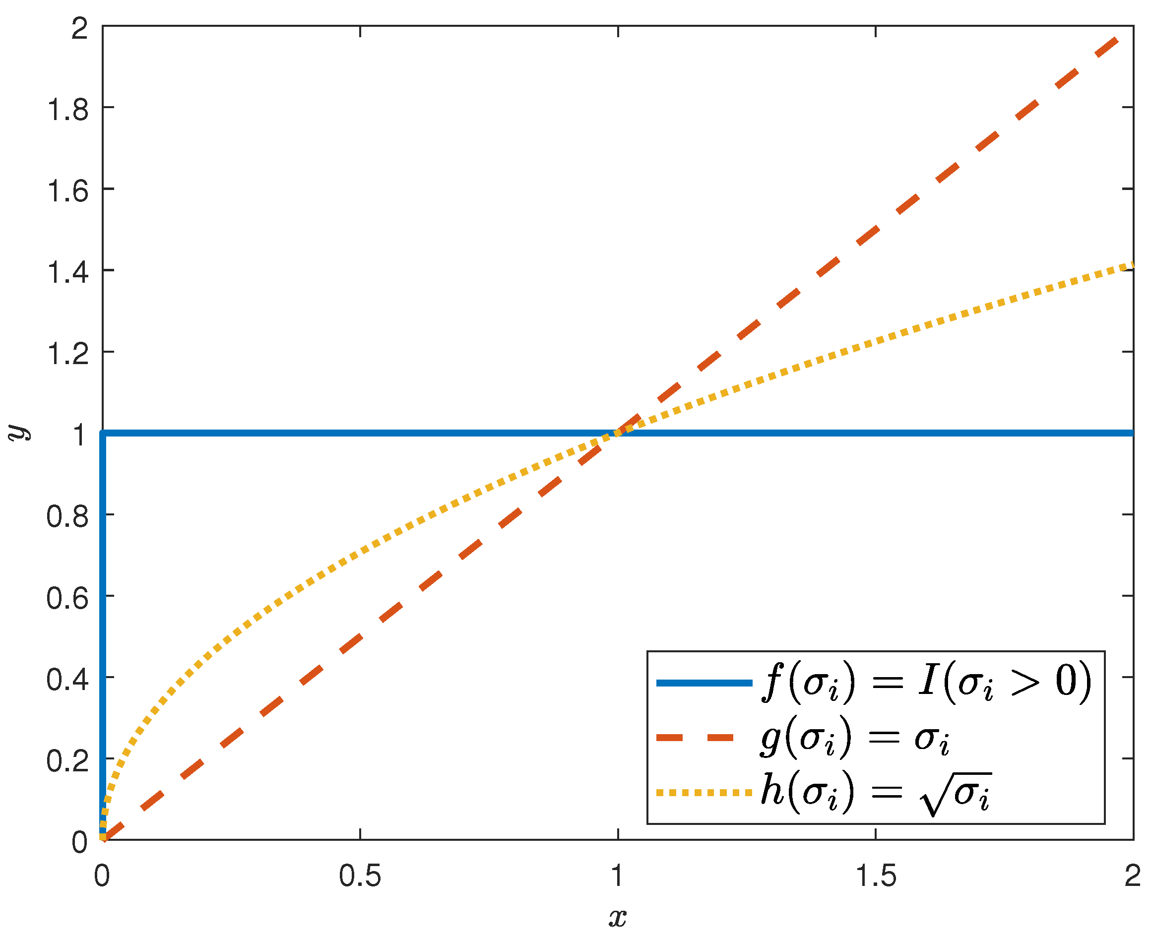
We propose the non-convex correlated total variation regularization term for simultaneously modeling the low-rank and local smoothness priors.

2.

We propose a hyperspectral image denoising algorithm based on our non-convex correlated total variation, demonstrating excellent denoising performance in scenarios with severe mixed noise.

The remainder of this article is structured as follows: Section 2 reviews relevant background knowledge and explains the motivation behind this study while also analyzing the low-rank models for hyperspectral image denoising; Section 3 presents the non-convex correlated total variation regularization (NCTV) and describes its application in hyperspectral image denoising; Section 4 reports the outcomes of our numerical experiments; finally, Section 5 summarizes the findings of this study.

2. Background and Motivation

As highlighted in the introduction, HSIs are inherently susceptible to complex noise contamination during acquisition [61,62]. This degradation arises from multiple sources, including sensor thermal fluctuations, photon shot noise, atmospheric scattering, and calibration errors, which manifest as mixed noise types such as Gaussian noise, impulse noise (i.e., sparse outliers), stripe noise (i.e., line artifacts), and dead-line noise (i.e., column-wise dropouts). The degradation model of a hyperspectral image can be expressed as the sum of a clean image $\mathit{X}$ and noise $\mathit{S}$, i.e., $\mathit{Y}=\mathit{X}+\mathit{S}$ [63]. Critically, the spectral correlation inherent to HSIs—stemming from the high redundancy between adjacent bands—endows the data with low-rank properties. This characteristic enables effective subspace regularization through low-rank constraints, as the intrinsic dimensionality of the clean HSI X is significantly lower than its ambient space defined by the spatial dimensions ($HW$) and spectral bands (B).

The theoretical foundation for exploiting this low-rank structure was established by Wright et al. [41] and Candès et al. [42], who introduced the RPCA framework. The RPCA model originally aimed to minimize the rank of the data. Due to the discreteness of the matrix rank, the solution to this problem is NP-hard [64]. To overcome this difficulty, a common method is to use convex relaxation [45,60,65], in which the rank is replaced with a nuclear norm in order to convert it into a convex optimization problem, as shown in Equation (2). The nuclear norm, defined as ${\parallel \mathit{X}\parallel }_{*}={\sum }_i{\sigma }_i$, linearly penalizes singular values, leading to uniform shrinkage across all magnitudes; however, this significantly differs from the rank function, which nonlinearly “counts” non-zero singular values via the step function:

$$\mathrm{Rank}\left(\mathit{X}\right)=\sum _{i}f\left({\sigma }_i\right)$$

(5)

where $f\left({\sigma }_i\right)$ represents the step function

$$f\left({\sigma }_i\right)=I({\sigma }_i>0)=\left\{\begin{array}{cc}1,\hfill & \mathrm{if}{\sigma }_i>0;\hfill \\ 0,\hfill & \mathrm{if}{\sigma }_i=0,\hfill \end{array}\right.$$

(6)

where $I({\sigma }_i>0)$ represents the indicator function about ${\sigma }_i>0$.

In fact, the definition of the nuclear norm can be rewritten as a function of singular values:  

$${\parallel \mathit{X}\parallel }_{*}=\sum _{i}g\left({\sigma }_i\right)$$

(7)

where $g\left({\sigma }_i\right)$ represents the identity mapping. Comparing Equations (5) and (7), when replacing the matrix rank by nuclear norms, an identity mapping is actually used to approximate the step function. As visualized in Figure 1, this approximation is suboptimal, particularly for larger singular values. This mismatch introduces a shrinkage bias in which dominant singular values that encode critical structural and spectral information are disproportionately penalized. Consequently, nuclear norm minimization risks oversmoothing details, thereby undermining the fidelity of the recovered HSI.

Although the correlated total variation (CTV) regularization term provides an innovative approach in unifying low-rank and local smoothness priors by applying the nuclear norm to gradient maps ${\nabla }_i\mathit{X}$, it still inherits this fundamental flaw. By imposing $\parallel {\nabla }_i{\mathit{X}\parallel }_{*}$, CTV propagates the shrinkage bias into the gradient domain, potentially erasing fine textures and edges. This limitation underscores the need for non-convex rank surrogates that can better approximate the step function.

In summary, while convex relaxation via the nuclear norm has enabled progress in HSI denoising, its inherent approximation errors necessitate advanced regularization strategies. Addressing these limitations forms the cornerstone of our proposed non-convex CTV framework, which is presented in the next section.

3. Method

3.1. Non-Convex Correlated Total Variation

According to the analysis in the previous section, we propose to utilize the low-rankness of the gradient graph of hyperspectral images for regularization, i.e., applying the nuclear norm $\parallel {\nabla }_i{\mathit{X}\parallel }_{*}$ to ${\nabla }_i\mathit{X}$. However, the nuclear norm has limitations in accurately estimating the rank. Essentially, this stems from the error generated by the identity mapping in approximating the step function. To address this issue, we employ the non-convex function $h\left({\sigma }_i\right)=\sqrt{{\sigma }_i}$ to approximate the identity mapping, which is the difference between our method NCVT and the previous CTV method. Figure 1 shows that $h\left({\sigma }_i\right)=\sqrt{{\sigma }_i}$ has a better approximation effect than $g\left({\sigma }_i\right)={\sigma }_i$. Although various non-convex functions exist, only regularization with the function $h\left({\sigma }_i\right)=\sqrt{{\sigma }_i}$ can derive a closed-form solution. This property permits explicit mathematical expression of the results and facilitates efficient algorithmic implementation. Based on this observation, we propose the following definition.

Definition 1 (Non-convex Correlation Total Variation). For a tensor $\mathcal{X}\in {\mathbb{R}}^{H\times W\times B}$, its matrix form is denoted as $\mathit{X}\in {\mathbb{R}}^{HW\times B}$. If ${\nabla }_i\mathit{X}$ ($i=1,2,3$) is the gradient map along the ith dimension, then the non-convex correlation total variation is defined as

$${\parallel \mathit{X}\parallel }_{\mathrm{NCTV}}={\displaystyle \frac{1}{3}}\sum _{i=1}^3{\parallel {\nabla }_i\mathit{X}\parallel }_{*,{\displaystyle \frac{1}{2}}},$$

(8)

where $\parallel {\nabla }_i{\mathit{X}\parallel }_{*,{\displaystyle \frac{1}{2}}}={\sum }_{i=1}^B\sqrt{{\sigma }_i}$ is the Schatten-${\displaystyle \frac{1}{2}}$ norm and $\mathbf{\sigma }=({\sigma }_1,{\sigma }_2,\dots ,{\sigma }_B)$ is the singular value of ${\nabla }_i\mathit{X}$.

HSIs can be represented in two forms, the matrix and the tensor; these two forms can be converted into each other using the reshape operation. While the form in the definition is a matrix, the algorithmic implementation first computes gradients along the three dimensions in tensor form. These tensor-based gradients are subsequently converted into matrix form in order to apply non-convex nuclear norm regularization, as the nuclear norm operator is defined for matrix-structured data.

3.2. Application of Non-Convex Correlation Total Variation in Hyperspectral Image Denoising

Based on the proposed non-convex correlation total variation and combined with the idea of robust principal component analysis, the following model is established:

$$\underset{\mathit{X},\mathit{S}}{min}{\parallel \mathit{X}\parallel }_{\mathrm{NCTV}}+\lambda {\parallel \mathit{S}\parallel }_1\mathrm{s}.\mathrm{t}.\mathit{Y}=\mathit{X}+\mathit{S}.$$

(9)

According to the definition of the non-convex correlation total variation, this can be rewritten as follows:

$$\underset{\mathit{X},\mathit{S}}{min}{\displaystyle \frac{1}{3}}\sum _{i=1}^3\parallel {\nabla }_i{\mathit{X}\parallel }_{*,{\displaystyle \frac{1}{2}}}+\lambda {\parallel \mathit{S}\parallel }_1\mathrm{s}.\mathrm{t}.\mathit{Y}=\mathit{X}+\mathit{S}.$$

(10)

Because the regularization term is applied to the discrete gradient of the data, auxiliary variables are introduced for decoupling:

$$\underset{\mathit{X},\mathit{S},{\mathit{G}}_{\mathit{I}}}{min}{\displaystyle \frac{1}{3}}\sum _{i=1}^3\parallel {\mathit{G}}_{\mathit{I}}{\parallel }_{*,{\displaystyle \frac{1}{2}}}+\lambda {\parallel \mathit{S}\parallel }_1\mathrm{s}.\mathrm{t}.\mathit{Y}=\mathit{X}+\mathit{S},{\mathit{G}}_{\mathit{I}}={\nabla }_i\mathit{X}.$$

(11)

Due to the objective function being non-convex and non-smooth, optimization is challenging; therefore, the alternating direction method of multipliers (ADMM) [66,67] is used to solve the optimization [68]. Based on the ADMM method, we first formulate the augmented Lagrangian function corresponding to the objective function, as follows:

$$\begin{array}{cc}\hfill \mathcal{L}(\mathit{X},\mathit{S},{\left\{{\Gamma }_i\right\}}_{i=1}^4,{\left\{{\mathit{G}}_i\right\}}_{i=1}^3)=& \sum _{i=1}^3\parallel {\mathit{G}}_i{\parallel }_{*}+{3\lambda \parallel \mathit{S}\parallel }_1+\sum _{i=1}^3{\displaystyle \frac{\mu }{2}}{\parallel {\nabla }_i\mathit{X}-{\mathit{G}}_i+{\displaystyle \frac{{\Gamma }_i}{\mu }}\parallel }_F^2\hfill \\ \hfill & +{\displaystyle \frac{\mu }{2}}{\parallel \mathit{Y}-\mathit{X}-\mathit{S}+{\displaystyle \frac{{\Gamma }_4}{\mu }}\parallel }_F^2\hfill \end{array}$$

(12)

where $\mu$ is the penalty parameter and ${\Gamma }_i$ ($i=1,2,3,4$) are the Lagrange multipliers.

Next, we discuss how to solve the subproblems for each variable.

1. Update ${\mathit{S}}^{k+1}$: Remove all variables except $\mathit{S}$ from the Lagrangian function, resulting in the following subproblem:

$$\underset{\mathit{S}}{min}{3\lambda \parallel \mathit{S}\parallel }_1+{\displaystyle \frac{\mu }{2}}{\parallel \mathit{Y}-\mathit{X}-\mathit{S}+{\displaystyle \frac{{\Gamma }_4}{\mu }}\parallel }_F^2.$$

(13)

The solution to the above problem can be expressed as ${\mathit{S}}^{k+1}=S_{3\lambda /\mu }(\mathit{Y}-{\mathit{X}}^k+{\Gamma }_4^k/\mu )$, where S is the soft thresholding operator.

2. Update $({\mathit{X}}^{k+1},{\mathit{G}}_i^{k+1})$: We first update ${\mathit{G}}_i$ by solving the following subproblem:

$$\underset{{\mathit{G}}_i}{min}\parallel {\mathit{G}}_i{\parallel }_{*}+{\displaystyle \frac{\mu }{2}}{\parallel {\mathit{G}}_i-({\nabla }_i{\mathit{X}}^k+{\displaystyle \frac{{\Gamma }_i^k}{\mu }})\parallel }_F^2.$$

(14)

The solution to this subproblem is as follows:

$$\left\{\begin{array}{c}{\mathit{G}}_i^{k+1}=\mathit{U}{H}_{1/\mu }(\Sigma ){\mathit{V}}^T\hfill \\ \mathit{U}\Sigma {\mathit{V}}^T=\mathrm{svd}({\nabla }_i{\mathit{X}}^k+{\Gamma }_i^k/\mu )\hfill \end{array}\right.$$

(15)

where  

$$H\left(x\right)=\left\{\begin{array}{cc}{\displaystyle \frac{2}{3}}x\left(1+cos\left({\displaystyle \frac{2\pi }{3}}-{\displaystyle \frac{2}{3}}{h}_{\gamma }\left(x\right)\right)\right),\hfill & \left|x\right|>{\displaystyle \frac{\sqrt[3]{54}}{4}}{\gamma }^{{\displaystyle \frac{2}{3}}}\hfill \\ 0,\hfill & \mathrm{otherwise}\hfill \end{array}\right.$$

(16)

$$h_{\gamma }\left(x\right)=arccos\left({\displaystyle \frac{\gamma }{8}}{\left({\displaystyle \frac{\left|x\right|}{3}}\right)}^{-3/2}\right).$$

(17)

Next, we update $\mathit{X}$ by solving the following subproblem:

$$\underset{\mathit{X}}{min}\sum _{i=1}^3{\displaystyle \frac{\mu }{2}}\parallel {\nabla }_i\mathit{X}-{\mathit{G}}_i^{k+1}+{\Gamma }_i^k{/\mu \parallel }_F^2+{\displaystyle \frac{\mu }{2}}{\parallel \mathit{Y}-\mathit{X}-{\mathit{S}}^{k+1}+{\Gamma }_4^k/\mu \parallel }_F^2.$$

(18)

Optimizing the above problem can be regarded as solving the following linear system:

$$\begin{array}{cc}\hfill (\mu \mathit{I}+\mu \sum _{i=1}^3{\nabla }_i^T{\nabla }_i)\left(\mathit{X}\right)& =\mu (\mathit{Y}-{\mathit{S}}^{k+1})+{\Gamma }_4^k+\mu \sum _{i=1}^3{\nabla }_i^T\left({\mathit{G}}_i^{k+1}\right)-{\nabla }_i^T\left({\Gamma }_i^k\right),\hfill \end{array}$$

(19)

where ${\nabla }_i^T(·)$ represents the transpose operator of ${\nabla }_i(·)$. Because the matrix corresponding to the operator ${\nabla }_i^T{\nabla }_i$ has a block-circulant structure, it can be diagonalized by performing Fourier transformation on both sides of the Lagrangian function. According to the convolution theorem, the closed-form solution for ${\mathit{X}}^{k+1}$ can be easily derived as follows:

$$\left\{\begin{array}{c}\mathit{H}=\sum _{i=1}^3\mathcal{F}{\left({\nabla }_i\right)}^{*}\odot \mathcal{F}(\mu {\mathit{G}}_i^{k+1}-{\Gamma }_i^k)\hfill \\ {\mathit{T}}_x=|\mathcal{F}\left({\nabla }_1\right){|}^2+|\mathcal{F}\left({\nabla }_2\right){|}^2+{\left|\mathcal{F}\left({\nabla }_3\right)\right|}^2\hfill \\ {\mathit{X}}^{k+1}={\mathcal{F}}^{-1}\left({\displaystyle \frac{\mathcal{F}(\mu \mathit{Y}-\mu {\mathit{S}}^{k+1}+{\Gamma }_4^k)+\mathit{H}}{\mu \mathbf{1}+\mu {\mathit{T}}_x}}\right)\hfill \end{array}\right.$$

(20)

where $\mathbf{1}$ represents a tensor with all elements equal to 1, ⊙ represents element-wise multiplication, $\mathcal{F}(·)$ represents the Fourier transform, and ${|·|}^2$ represents the element-wise square operation.

3. Update the multipliers ${\Gamma }_i^{k+1}$, $i=1,2,3,4$: Based on the ADMM principle, the multipliers are further updated using the following equations:

$$\left\{\begin{array}{c}{\Gamma }_i^{k+1}={\Gamma }_i^k+\mu ({\nabla }_i{\mathit{X}}^{k+1}-{\mathit{G}}_i^{k+1}),i=1,2,3\hfill \\ {\Gamma }_4^{k+1}={\Gamma }_4^k+\mu (\mathit{Y}-{\mathit{X}}^{k+1}-{\mathit{S}}^{k+1})\hfill \\ \mu =\mu \rho \hfill \end{array}\right.$$

(21)

where $\rho$ is a constant that is greater than 1.

Algorithm 1 summarizes the workflow, while Figure 2 shows the flow of the algorithm.

Algorithm 1 ADMM Algorithm Process

Require:  Noisy hyperspectral image $\mathcal{Y}\in {\mathbb{R}}^{H\times W\times B}$, its matrix form $\mathit{Y}\in {\mathbb{R}}^{HW\times B}$, $\mu ={10}^{-6}$, $ϵ={10}^{-6}$ Ensure:  $\mathit{X}$ 1: Initialize $\mathit{S}=\mathbf{0}$. 2: Initialize $\mathit{X}$ randomly through a standard normal distribution. 3: while not converged do 4:    Update ${\mathit{G}}_i^{k+1}$. 5:    Update ${\mathit{S}}^{k+1}$. 6:    Update ${\mathit{X}}^{k+1}$. 7:    Update ${\Gamma }_i^{k+1}$. 8:    Update $\mu =\rho \mu$. 9:    Update $k:=k+1$. 10:    if $\parallel \mathit{Y}-{\mathit{X}}^{k+1}-{\mathit{S}}^{k+1}{\parallel }_F^2/{\parallel \mathit{Y}\parallel }_F^2\le ϵ$ and $\parallel {\nabla }_i{\mathit{X}}^{k+1}-{\mathit{G}}_i^{k+1}{\parallel }_F^2/{\parallel \mathit{Y}\parallel }_F^2\le ϵ$ then 11:      BREAK 12:    end if 13: end while

4. Experiments

This study included comprehensive experiments to validate the effectiveness of the proposed non-convex correlated total variation method and compare the results with existing hyperspectral image denoising methods. Prior to denoising, the grayscale values of each band were scaled proportionally to the range $[0,1]$ and subsequently restored to their original dynamic range in postprocessing. All experiments were performed using MATLAB R2022a on a laptop computer.

The compared methods are briefly introduced below along with their respective parameter settings.

1.

NMoG (non-i.i.d. mixture of Gaussians) [69]: The NMoG method models the noise within each spectral band using a distinct MoG distribution and imposes hierarchical priors on the MoG parameters. The parameters were set as follows: target rank of the low-rank component = 5, initial rank of the low-rank component = 30, rank reduction per iteration = 7, Gaussian mixture components reduced per band = 1, maximum number of iterations = 30, and convergence tolerance = ${10}^{-4}$.

2.

NGMeet (non-local meets global) [70]: NGMeet proposes a unified spatial–spectral denoising paradigm that jointly models the global spectral low-rank property (via an orthogonal basis and reduced image) and spatial non-local similarity (via low-rank regularization on the reduced image).

3.

LRTV (low-rank total variation) [46]: LRTV integrates nuclear norm minimization for spectral low-rank property, total variation regularization for spatial smoothness, and $l_1$-norm regularization for sparse noise separation within a unified framework. The parameters in this method were set as follows: when the number of bands exceeded 100, the $\tau$ parameter was set to $0.015$, $\lambda$ to $20/\sqrt{MN}$, and the target rank to 10. When the number of bands did not exceed 100, the $\tau$ parameter was set to $0.01$, $\lambda$ to $10/\sqrt{MN}$, and the target rank to 5.

4.

CTV (correlated total variation) [54]: CTV regularization captures the joint low-rankness and local smoothness by applying the nuclear norm to the gradient maps of the data. The $\rho$ parameter was set to $1.5$.

5.

3DTNN (three-directional tensor nuclear norm) [71]: 3DTNN employs a convex three-directional tensor nuclear norm as a regularizer to enforce low-rankness across all modes of the hyperspectral image tensor. The standard deviation of random noise was set to a uniform distribution between 0 and $70/255$, while the $\theta$ parameter was set to $0.001$, the $\varphi$ parameter to $0.004$, the $\varpi$ parameter to 1, and the $\omega$ parameter to 100.

6.

3DLogTNN (three-directional log-based tensor nuclear norm) [71]: This model employs a non-convex logarithmic function to approximate the rank by penalizing singular values differently across three directional tensor nuclear norms. The standard deviation of random noise was set to a uniform distribution between 0 and $70/255$. The $\theta$ parameter was set to $0.001$, the $\varphi$ parameter to $0.00005$, the $\varpi$ parameter to $0.011$, and the $\omega$ parameter to 10,000. Finally, the logarithmic tolerance was set to 80.

7.

WNLRATV (weighted non-local low-rank model with adaptive total variation regularization) [72]: WNLRATV integrates a weighted term based on non-i.i.d. mixture-of-Gaussian noise modeling, a non-local low-rank tensor prior, and an adaptive edge-preserving total variation regularization for denoising. The parameters in this method were set as follows: the initial rank was set to 3, the target rank to 6, the $\alpha$ parameter to 30, the $\beta$ parameter to 1, the $\gamma$ parameter to $0.08$, the maximum iteration to 15, the patch number to 200, and the $\lambda$ parameter to $0.2$.

8.

BALMF (band-wise asymmetric Laplacian noise modeling matrix factorization) [63]: BALMF models the hyperspectral image noise per band using an asymmetric Laplacian distribution within a low-rank matrix factorization framework. The r parameter was set to 4.

4.1. Simulation Results and Analysis

4.1.1. Data Simulation

In this section, we first compare the denoising effects of different methods on images containing mixed noise. The selected datasets included Reno_256_128 and WDCMall, with image sizes of $256\times 256\times 128$ and $200\times 200\times 160$, respectively. The pixel values of all images were normalized to the range $[0,1]$. In this experiment, six types of noise were considered, described briefly as follows:

1.

Gaussian noise with a standard deviation of $25/255$ is added following an independent and identically distributed (i.i.d.) pattern.

2.

Non-i.i.d. Gaussian noise is added with a standard deviation randomly distributed between $10/255$ and $70/255$.

3.

On the basis of noise type 2, impulse noise is randomly added to $1/3$ of the bands, with the noise intensity randomly distributed between $0.05$ and $0.2$.

4.

On the basis of noise type 2, stripe noise is randomly added to $1/3$ of the bands, with the noise intensity randomly distributed between $0.05$ and $0.2$.

5.

On the basis of noise type 2, $1/3$ of the bands are randomly selected for added dead-line noise, with the noise intensity randomly distributed between $0.05$ and $0.2$.

6.

On the basis of noise type 2, $1/3$ of the bands are randomly selected for added mixed noise consisting of impulse noise, stripe noise, and dead-line noise, with the noise intensity randomly distributed between $0.05$ and $0.2$ for all types.

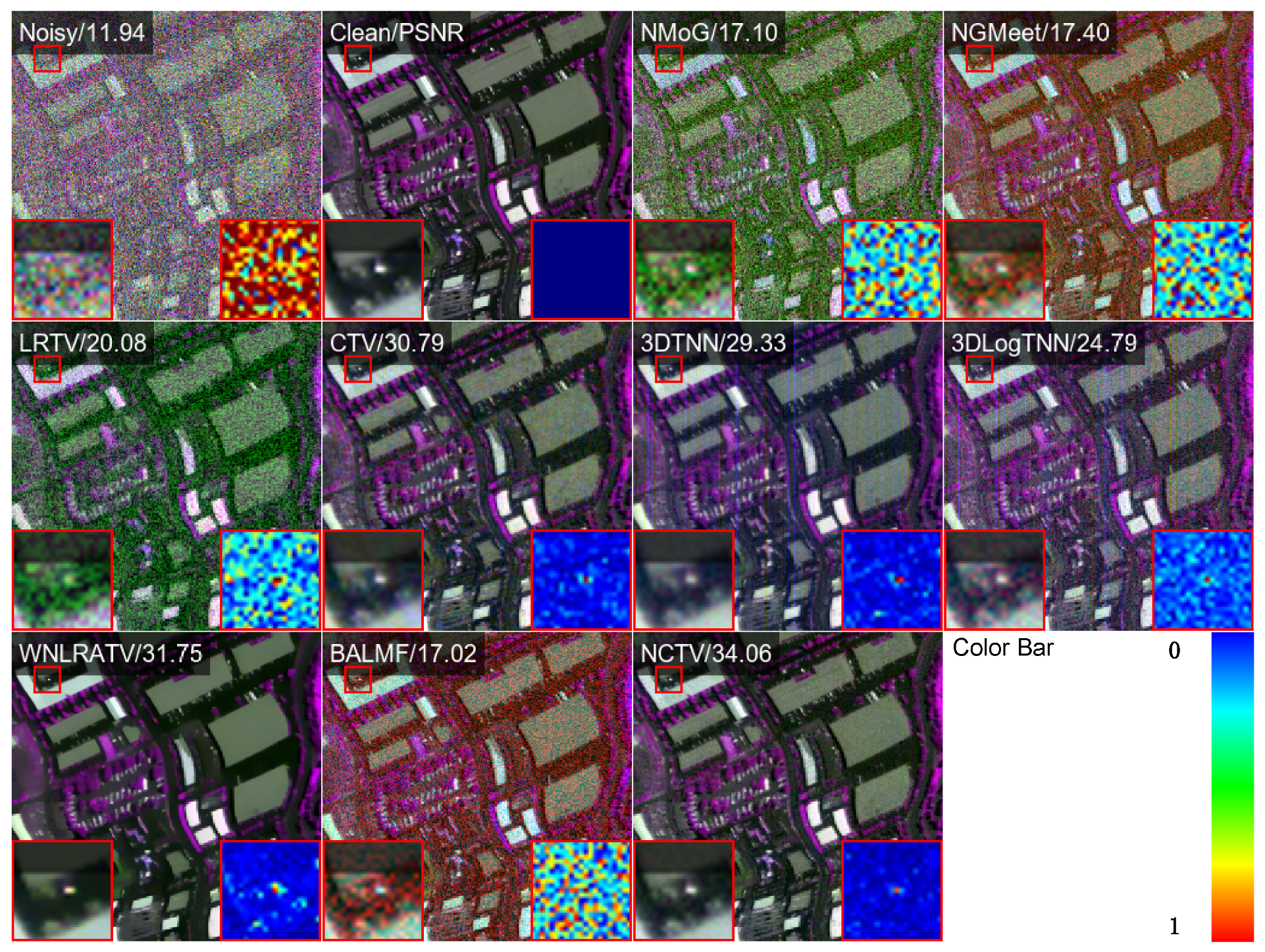
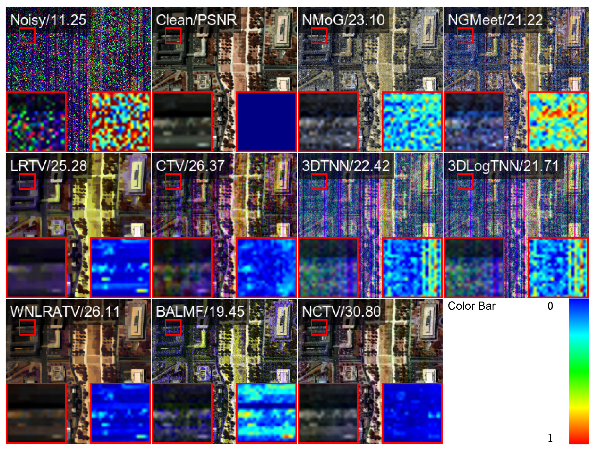
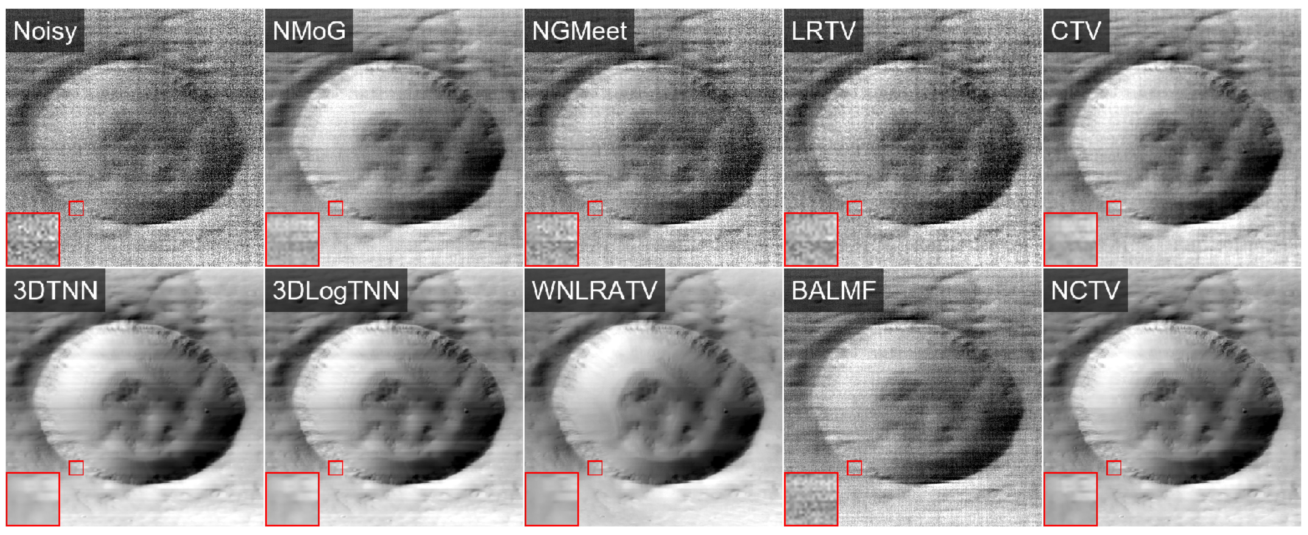
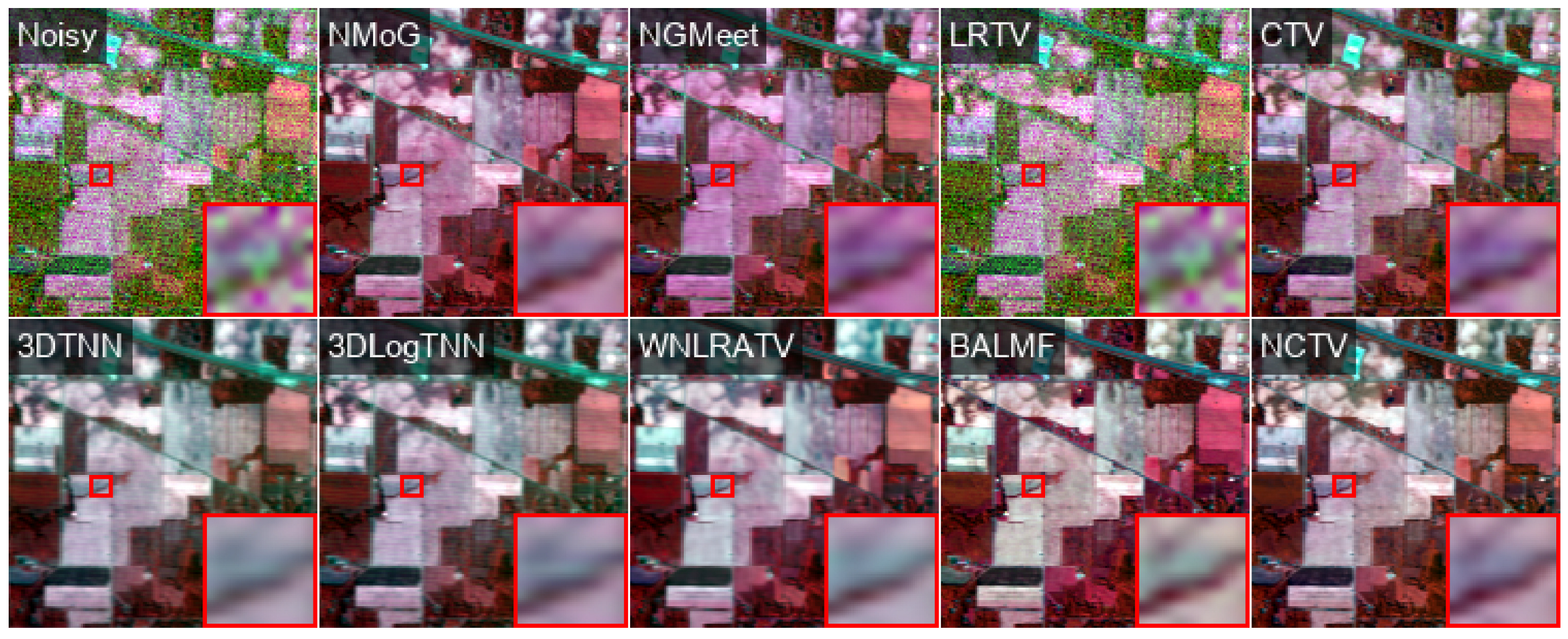
4.1.2. Results Analysis

Four quantitative metrics were adopted for evaluation: the peak signal-to-noise ratio (PSNR), structural similarity index (SSIM), error relative to global variance (ERGAS), and spectral angle mapper (SAM). Typically, the denoised image will be closer to the original image if the first two metrics are higher and the last two metrics are lower, indicating better denoising performance.

Examples of typical bands of denoised images obtained by the different methods are shown in Figure 3 and Figure 4. For the results of case 4 in Figure 3, it can be seen in the images that the results from methods such as NMoG, NGMeet, LRTV, and BALMF still contain noticeable dot pattern noise. Moreover, upon magnification of the micrographs, it is apparent that the result obtained by our non-convex total variation (NCTV) method is the closest to the true image and that the residual is relatively minimal, resulting in the best denoising effect. For the results of case 6 in Figure 4, the results from methods such as NMoG, NGMeet, 3DTNN, 3DLogTNN, and BALMF still contain dot pattern impulse noise and line stripe noise, while the magnified micrographs show that the denoising effect of our NCTV method is better. Therefore, compared with other denoising methods, our proposed method achieves the best visual effect in this simulation scenario.

Table 1. Metrics on the Reno_256_128 dataset. The best results are in bold and the second-best results are in red. The column on the far right is the NCTV method proposed in this paper.

Cases of the Noise	Metrics	Noisy	NMoG	NGMeet	LRTV	CTV	3DTNN	3DLogTNN	WNLRATV	BALMF	NCTV
1	PSNR	20.17	35.23	39.24	32.81	34.03	34.45	36.02	36.57	33.22	35.58
	SSIM	0.3747	0.9371	0.9758	0.8983	0.9136	0.9522	0.9572	0.9541	0.889	0.9436
	ERGAS	317.43	57.31	35.46	76.44	64.23	61.22	51.25	48.26	71.81	55.21
	SAM	23.95	3.73	2.04	4.26	4.5	3.03	2.82	2.89	4.99	3.33
2	PSNR	16.87	34.59	31.67	30.85	31.78	32.27	33.87	33.01	31.85	33.96
	SSIM	0.2696	0.9265	0.8683	0.8512	0.8629	0.9258	0.9186	0.915	0.8826	0.9198
	ERGAS	559.41	61.76	130.8	117.09	85.29	79.15	68.46	76.86	118.08	66.07
	SAM	37.13	4.06	9.85	7.6	6.09	3.74	4.22	4.65	9.45	3.88
3	PSNR	15.86	31.67	29.81	30.12	32.05	31.99	34.07	33.92	30.24	34.12
	SSIM	0.2418	0.8886	0.8378	0.8358	0.8682	0.9242	0.9283	0.9274	0.8693	0.921
	ERGAS	629.76	150.72	162.04	156.77	83.34	82.54	66.66	71.37	155.56	64.24
	SAM	38.31	10.16	10.84	11.4	5.98	3.81	3.95	4.23	11.33	3.71
4	PSNR	16.35	33.03	31.49	30.38	31.17	30.72	30.81	31.58	31.31	33.56
	SSIM	0.2509	0.9015	0.8694	0.8413	0.8463	0.8722	0.8377	0.8806	0.867	0.9106
	ERGAS	575.66	115.38	139.97	133.17	92.03	100.14	113.61	98.71	129.88	69
	SAM	37.91	8.55	10.2	9.5	6.62	6.26	8.41	5.86	9.77	4.04
5	PSNR	16.01	30.06	28.84	27.33	27.48	27.08	26.46	29.26	28.15	29.63
	SSIM	0.2375	0.8891	0.8396	0.7659	0.7559	0.7323	0.68	0.8541	0.7814	0.8695
	ERGAS	585.57	156.39	169.36	217.42	188.62	230.21	250.54	141.23	225.14	150.13
	SAM	39.9	10.56	11.61	14.91	13.85	15.96	18.4	7.42	15.54	10.19
6	PSNR	14.36	27.77	27.3	27.15	26.97	25.94	25.7	28.78	26.54	29.24
	SSIM	0.1911	0.8371	0.8222	0.7599	0.7409	0.7102	0.6721	0.8439	0.7484	0.8634
	ERGAS	690.46	202.48	189.33	225.61	195.79	243.66	257.79	146.98	259.12	154.53
	SAM	42.42	13.06	12.84	15.25	14.32	17.06	19.08	8.19	18.06	10.35

and

Table 2. Metrics on the WDCMall dataset. The best results are in bold and the second-best results are in red. The column on the far right is the NCTV method proposed in this paper.

Cases of the Noise	Metrics	Noisy	NMoG	NGMeet	LRTV	CTV	3DTNN	3DLogTNN	WNLRATV	BALMF	NCTV
1	PSNR	20.17	35.53	38.01	32.05	33.57	33.64	35.22	34.72	33.74	35.36
	SSIM	0.5223	0.9695	0.9829	0.9232	0.9496	0.9668	0.9714	0.9639	0.9523	0.9699
	ERGAS	368.76	60.9	45.26	91.87	76.59	75.3	63.04	65.8	75.4	64.27
	SAM	26.86	5.27	3.37	5.75	6.48	4.4	4.56	3.79	6.54	4.92
2	PSNR	16.73	34.01	31.37	29.78	31.04	28.15	26.63	31.24	31.48	33.42
	SSIM	0.3732	0.9566	0.9238	0.872	0.9106	0.823	0.7608	0.9176	0.9287	0.9536
	ERGAS	638.64	78.98	123.64	152.34	105.6	156.25	209.98	98.53	112.24	80.37
	SAM	38.9	7.29	11.15	11.63	8.76	12.42	17.52	5.17	10.19	5.95
3	PSNR	15.74	31.17	28.86	29.92	31.62	28.33	27.28	32.08	30.35	33.84
	SSIM	0.3448	0.9147	0.8675	0.8766	0.918	0.8202	0.7716	0.9278	0.8933	0.9591
	ERGAS	781.42	180.49	221.46	166.92	100.18	159.33	207.53	93.8	157.62	76.13
	SAM	40.38	11.2	13.67	12.06	7.88	11.93	16.15	5.63	9.92	5.24
4	PSNR	16.44	34.16	30.97	29.54	30.8	28.87	28.16	31.54	31.57	33.37
	SSIM	0.3646	0.9602	0.9115	0.8695	0.9074	0.8654	0.8292	0.9212	0.9225	0.954
	ERGAS	660.02	70.94	133.14	161.59	106.49	141.18	167.41	96.14	97.23	78.18
	SAM	39.79	6.05	11.18	12.78	8.89	10.56	13.97	5.52	8.55	5.91
5	PSNR	16.3	31.12	28.86	27.15	27.95	26.8	27.14	29.15	29.13	29.88
	SSIM	0.3568	0.9414	0.8989	0.8212	0.8454	0.8045	0.7979	0.8921	0.8703	0.9141
	ERGAS	679.36	141.75	171.92	231.82	189.1	246.81	252.03	149.13	199.12	153.49
	SAM	42.28	10.12	12.92	16.96	14.81	18.08	19.79	7.99	14.14	11.18
6	PSNR	14.46	27.8	26.67	26.91	27.37	23.25	22.08	28.56	27.03	29.39
	SSIM	0.2865	0.8819	0.8509	0.7992	0.8269	0.646	0.5961	0.8642	0.7992	0.9084
	ERGAS	826.68	210.11	230.92	244.93	196.95	313.68	360.36	182.72	260.23	156.2
	SAM	44.13	14.11	15.52	17.24	14.74	22.83	26.56	9.66	15.66	10.74

summarize the performance of all competing methods in terms of PSNR, SSIM, ERGAS, and SAM on the Reno_256_128 and WDCMall datasets. It can be observed that our NCTV method achieves the best or second-best metrics under almost all noise conditions. In particular, our method obtains the best results on both datasets under mixed complex noise conditions, implying that it may perform better in real-world scenarios. Moreover, the results of our method are the most stable when comprehensively considering all noise conditions, verifying the effectiveness of non-convex total variation in removing mixed noise.

To further compare the differences among various methods, Figure 5 displays the PSNR values for each band of the denoised images. The Reno_256_128 dataset with noise type 3 and the WDCMall dataset with noise type 6 are shown, while the PSNR curves are displayed in Figure 5a,b. The curves reveal that the PSNR values of the NCTV method are relatively high on most bands compared to the other methods, indicating that the superior denoising effect of NCTV.

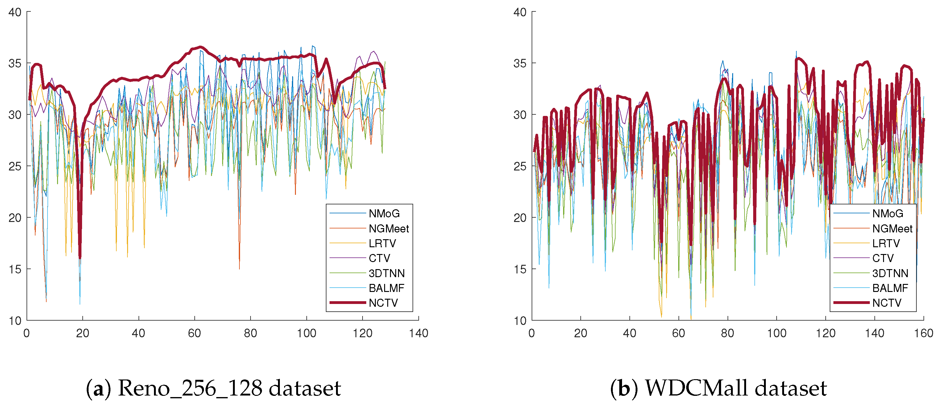
4.2. Experiments on Real-World Datasets

In the real-world experiment, we used the Mars and Indian_Pines hyperspectral images as real datasets and tested our denoising method against other existing methods. The Mars hyperspectral image was captured and cropped into blocks of size $400\times 400$ with 102 channels, while the Indian_Pines hyperspectral image was captured and cropped into blocks of size $145\times 145$, with 206 channels.

The results of the denoised hyperspectral images are shown in Figure 6 and Figure 7. It can be observed that the denoising effects of the NMoG, NGMeet, LRTV, CTV, and BALMF methods are not satisfactory, as there are still various levels of impulse and stripe noises in the images. The NCTV method proposed in this project provides better denoising performance compared with most methods, especially in terms of impulse and stripe noise. The result also show that NCTV restores a majority of details and maintains color consistency with the original image.

4.3. Model Analysis

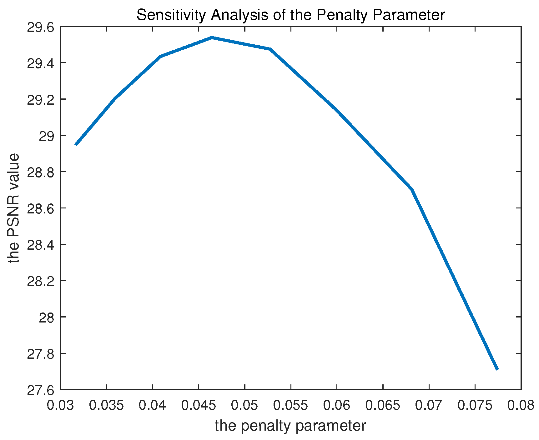
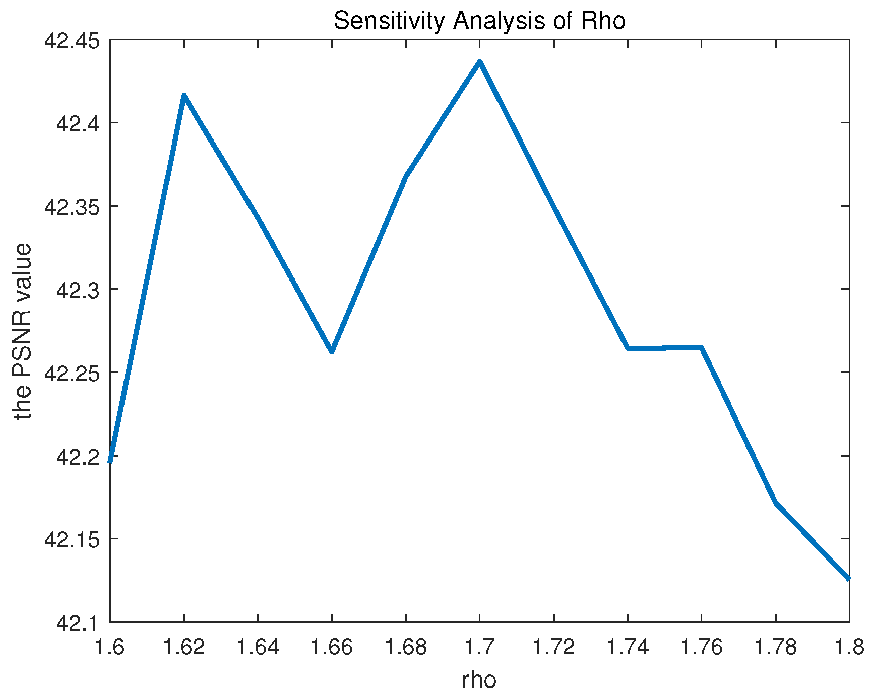
4.3.1. Parameter Sensitivity

This section analyzes the selection and setting of the model parameters of our NCTV method, specifically the penalty parameter $\lambda$ and hyperparameter $\rho$, in order to examine its sensitivity. Through a robust principal component analysis, the optimal parameter can be proven to be ${\lambda }^{*}=1/\sqrt{HW}$. However, the NCTV method proposed in this study deviates from the assumptions of robust principal component analysis, requiring adjustment of the $\lambda$ parameter. Based on experience, $\lambda$ can be set to $s/\sqrt{HW}$ in order to further adjust the s parameter. In a grid search experiment, we took uniform sampling points in the interval $[{10}^{-1.5},{10}^{-1}]$ as candidate values for the s parameter. On the other hand, previous studies usually set $\rho$ to $1.5$; thus, we tried to find the optimal parameter near $1.5$. In a grid search experiment, uniform sampling points were taken in the interval $[1.6,1.8]$ as candidate values for the hyperparameter $\rho$.

To examine the impact of the parameter $\lambda$ and hyperparameter $\rho$, we implemented NCTV on the WDCMall dataset. As depicted in Figure 8, the PSNR curve gradually increases before gradually descending as $\lambda$ increases, achieving the optimal performance when $\lambda$ is around 0.05. On the other hand, Figure 9 indicates that the optimal hyperparameter $\rho$ value is around 1.7.

4.3.2. Processing Time

Table 3. Processing times on the dataset Reno_256_128 in all cases (in seconds).

Methods	Case1	Case2	Case3	Case4	Case5	Case6
NMoG	88.46	127.22	115.96	108.67	104.06	138.45
NGMeet	143.90	125.23	128.43	118.65	123.90	174.14
LRTV	85.89	90.18	103.39	94.78	93.25	103.40
CTV	145.89	150.53	173.55	162.89	157.76	162.34
3DTNN	215.74	301.84	279.58	265.59	260.54	349.90
3DLogTNN	381.56	409.09	399.21	366.45	356.73	473.65
WNLRATV	948.94	811.66	967.99	911.02	915.61	1091.36
BALMF	215.75	153.76	208.99	208.10	209.64	225.33
NCTV	178.76	132.49	138.10	135.01	141.77	211.23

illustrates the processing time of different methods on the Reno_256_128 dataset. NMoG and LRTV are the fastest methods; however, as described before, the denoising performance of these methods is not as good as our NCTV method. Although our method is not the fastest, it provides better denoising results. In particular, although the denoising effect of the WNLRATV method is satisfactory, its processing time is much longer, meaning that its efficiency is relatively lower than that of our NCTV method.

5. Conclusions

In conclusion, our proposed denoising method for hyperspectral images based on the non-convex total variation (NCTV) demonstrates superior performance compared to other existing methods when handling images with mixed noise containing Gaussian, impulse, stripe, and dead-line noise. Through simulation experiments on the Reno_256_128 and WDCMall datasets and using PSNR, SSIM, ERGAS, and SAM as evaluation metrics for assessment, our results indicate that the proposed NCTV method can effectively remove noise while largely preserving the texture and detail of the images. The results using the proposed NCTV method are more stable under different noise conditions. Additionally, although the processing time of our method is not the best, its denoising results are superior in terms of both visual effect and metrics when compared to the NMoG, NGMeet, LRTV, CTV, 3DTNN, 3DLogTNN, and BALMF methods. Through a parameter sensitivity analysis, we determined the optimal range for the penalty parameter $\lambda$ and hyperparameter $\rho$. In summary, the proposed non-convex total variation denoising method provides an effective technical approach for the field of hyperspectral image denoising. Although our model possesses the aforementioned advantages, there remains room for improvement in certain aspects. The performance and efficiency could be further enhanced; in addition, future work could refine the model architecture and accelerate the algorithm.

References

1. Plaza, A.; Benediktsson, J.A.; Boardman, J.W.; Brazile, J.; Bruzzone, L.; Camps-Valls, G.; Chanussot, J.; Fauvel, M.; Gamba, P.; Gualtieri, A.; et al. Recent advances in techniques for hyperspectral image processing. Remote Sens. Environ. 2009, 113, S110–S122, Imaging Spectroscopy Special Issue. [Google Scholar] [CrossRef]
2. Haboudane, D.; Miller, J.R.; Pattey, E.; Zarco-Tejada, P.J.; Strachan, I.B. Hyperspectral vegetation indices and novel algorithms for predicting green LAI of crop canopies: Modeling and validation in the context of precision agriculture. Remote Sens. Environ. 2004, 90, 337–352. [Google Scholar] [CrossRef]
3. Hu, Y.; Li, X.; Gu, Y.; Jacob, M. Hyperspectral Image Recovery Using Nonconvex Sparsity and Low-Rank Regularizations. IEEE Trans. Geosci. Remote Sens. 2020, 58, 532–545. [Google Scholar] [CrossRef]
4. Chen, Y.; Guo, Y.; Wang, Y.; Wang, D.; Peng, C.; He, G. Denoising of Hyperspectral Images Using Nonconvex Low Rank Matrix Approximation. IEEE Trans. Geosci. Remote Sens. 2017, 55, 5366–5380. [Google Scholar] [CrossRef]
5. Lu, H.; Yang, Y.; Huang, S.; Tu, W.; Wan, W. A Unified Pansharpening Model Based on Band-Adaptive Gradient and Detail Correction. IEEE Trans. Image Process. 2022, 31, 918–933. [Google Scholar] [CrossRef] [PubMed]
6. Yang, Y.; Tu, W.; Huang, S.; Lu, H.; Wan, W.; Gan, L. Dual-Stream Convolutional Neural Network With Residual Information Enhancement for Pansharpening. IEEE Trans. Geosci. Remote. Sens. 2022, 60, 5402416. [Google Scholar] [CrossRef]
7. Zhang, H.; He, W.; Zhang, L.; Shen, H.; Yuan, Q. Hyperspectral Image Restoration Using Low-Rank Matrix Recovery. IEEE Trans. Geosci. Remote Sens. 2014, 52, 4729–4743. [Google Scholar] [CrossRef]
8. Sun, K.; Zhang, J.; Xu, S.; Zhao, Z.; Zhang, C.; Liu, J.; Hu, J. CACNN: Capsule Attention Convolutional Neural Networks for 3D Object Recognition. IEEE Trans. Neural Netw. Learn. Syst. 2025, 36, 4091–4102. [Google Scholar] [CrossRef] [PubMed]
9. Bai, H.; Zhao, Z.; Zhang, J.; Wu, Y.; Deng, L.; Cui, Y.; Jiang, B.; Xu, S. ReFusion: Learning Image Fusion from Reconstruction with Learnable Loss Via Meta-Learning. Int. J. Comput. Vis. 2025, 133, 2547–2567. [Google Scholar] [CrossRef]
10. Bai, H.; Zhao, Z.; Zhang, J.; Jiang, B.; Deng, L.; Cui, Y.; Xu, S.; Zhang, C. Deep Unfolding Multi-Modal Image Fusion Network via Attribution Analysis. IEEE Trans. Circuits Syst. Video Technol. 2025, 35, 3498–3511. [Google Scholar] [CrossRef]
11. Xu, S.; Amira, O.; Liu, J.; Zhang, C.; Zhang, J.; Li, G. HAM-MFN: Hyperspectral and Multispectral Image Multiscale Fusion Network With RAP Loss. IEEE Trans. Geosci. Remote Sens. 2020, 58, 4618–4628. [Google Scholar] [CrossRef]
12. Wang, C.; Pedrycz, W.; Li, Z.; Zhou, M. Residual-driven Fuzzy C-Means Clustering for Image Segmentation. IEEE CAA J. Autom. Sin. 2021, 8, 876–889. [Google Scholar] [CrossRef]
13. Chen, Y.; Lai, W.; He, W.; Zhao, X.; Zeng, J. Hyperspectral Compressive Snapshot Reconstruction via Coupled Low-Rank Subspace Representation and Self-Supervised Deep Network. IEEE Trans. Image Process. 2024, 33, 926–941. [Google Scholar] [CrossRef] [PubMed]
14. Chen, Y.; Chen, M.; He, W.; Zeng, J.; Huang, M.; Zheng, Y. Thick Cloud Removal in Multitemporal Remote Sensing Images via Low-Rank Regularized Self-Supervised Network. IEEE Trans. Geosci. Remote Sens. 2024, 62, 5506613. [Google Scholar] [CrossRef]
15. Manolakis, D.; Shaw, G. Detection algorithms for hyperspectral imaging applications. IEEE Signal Process. Mag. 2002, 19, 29–43. [Google Scholar] [CrossRef]
16. Iordache, M.D.; Bioucas-Dias, J.M.; Plaza, A. Sparse Unmixing of Hyperspectral Data. IEEE Trans. Geosci. Remote Sens. 2011, 49, 2014–2039. [Google Scholar] [CrossRef]
17. Cerra, D.; Müller, R.; Reinartz, P. Noise Reduction in Hyperspectral Images Through Spectral Unmixing. IEEE Geosci. Remote Sens. Lett. 2014, 11, 109–113. [Google Scholar] [CrossRef]
18. Xu, S.; Ke, Q.; Peng, J.; Cao, X.; Zhao, Z. Pan-Denoising: Guided Hyperspectral Image Denoising via Weighted Represent Coefficient Total Variation. IEEE Trans. Geosci. Remote Sens. 2024, 62, 5528714. [Google Scholar] [CrossRef]
19. Zhang, Q.; Zheng, Y.; Yuan, Q.; Song, M.; Yu, H.; Xiao, Y. Hyperspectral Image Denoising: From Model-Driven, Data-Driven, to Model-Data-Driven. IEEE Trans. Neural Netw. Learn. Syst. 2024, 35, 13143–13163. [Google Scholar] [CrossRef]
20. Zhang, Q.; Yuan, Q.; Li, J.; Sun, F.; Zhang, L. Deep spatio-spectral Bayesian posterior for hyperspectral image non-i.i.d. noise removal. ISPRS J. Photogramm. Remote Sens. 2020, 164, 125–137. [Google Scholar] [CrossRef]
21. Zhang, Q.; Yuan, Q.; Li, J.; Liu, X.; Shen, H.; Zhang, L. Hybrid Noise Removal in Hyperspectral Imagery With a Spatial–Spectral Gradient Network. IEEE Trans. Geosci. Remote Sens. 2019, 57, 7317–7329. [Google Scholar] [CrossRef]
22. Yuan, Q.; Zhang, Q.; Li, J.; Shen, H.; Zhang, L. Hyperspectral Image Denoising Employing a Spatial–Spectral Deep Residual Convolutional Neural Network. IEEE Trans. Geosci. Remote Sens. 2019, 57, 1205–1218. [Google Scholar] [CrossRef]
23. Liu, W.; Lee, J. A 3-D Atrous Convolution Neural Network for Hyperspectral Image Denoising. IEEE Trans. Geosci. Remote Sens. 2019, 57, 5701–5715. [Google Scholar] [CrossRef]
24. Chen, H.; Yang, G.; Zhang, H. Hider: A Hyperspectral Image Denoising Transformer With Spatial–Spectral Constraints for Hybrid Noise Removal. IEEE Trans. Neural Netw. Learn. Syst. 2024, 35, 8797–8811. [Google Scholar] [CrossRef]
25. Zhang, Q.; Yuan, Q.; Song, M.; Yu, H.; Zhang, L. Cooperated Spectral Low-Rankness Prior and Deep Spatial Prior for HSI Unsupervised Denoising. IEEE Trans. Image Process. 2022, 31, 6356–6368. [Google Scholar] [CrossRef] [PubMed]
26. Shi, K.; Peng, J.; Gao, J.; Luo, Y.; Xu, S. Hyperspectral Image Denoising via Double Subspace Deep Prior. IEEE Trans. Geosci. Remote Sens. 2024, 62, 5531015. [Google Scholar] [CrossRef]
27. Lu, X.; Wang, Y.; Yuan, Y. Graph-regularized low-rank representation for destriping of hyperspectral images. IEEE Trans. Geosci. Remote Sens. 2013, 51, 4009–4018. [Google Scholar] [CrossRef]
28. Yuan, F.; Chen, Y.; He, W.; Zeng, J. Feature Fusion-Guided Network With Sparse Prior Constraints for Unsupervised Hyperspectral Image Quality Improvement. IEEE Trans. Geosci. Remote Sens. 2025, 63, 5511912. [Google Scholar] [CrossRef]
29. Liu, X.; Bourennane, S.; Fossati, C. Denoising of hyperspectral images using the PARAFAC model and statistical performance analysis. IEEE Trans. Geosci. Remote Sens. 2012, 50, 3717–3724. [Google Scholar] [CrossRef]
30. Li, C.; Ma, Y.; Huang, J.; Mei, X.; Ma, J. Hyperspectral image denoising using the robust low-rank tensor recovery. J. Opt. Soc. Am. A 2015, 32, 1604–1612. [Google Scholar] [CrossRef]
31. Renard, N.; Bourennane, S.; Blanc-Talon, J. Denoising and dimensionality reduction using multilinear tools for hyperspectral images. IEEE Geosci. Remote Sens. Lett. 2008, 5, 138–142. [Google Scholar] [CrossRef]
32. Wang, Y.; Xu, S.; Cao, X.; Ke, Q.; Ji, T.; Zhu, X. Hyperspectral Denoising Using Asymmetric Noise Modeling Deep Image Prior. Remote Sens. 2023, 15, 1970. [Google Scholar] [CrossRef]
33. Wu, J.M.; Yin, S.B.; Jiang, T.X.; Liu, G.S.; Zhao, X.L. PALADIN: A novel plug-and-play 3D CS-MRI reconstruction method. Inverse Probl. 2025, 41, 035014. [Google Scholar] [CrossRef]
34. Xu, S.; Zhang, J.; Wang, J.; Sun, K.; Zhang, C.; Liu, J.; Hu, J. A model-driven network for guided image denoising. Inf. Fusion 2022, 85, 60–71. [Google Scholar] [CrossRef]
35. Xu, S.; Peng, J.; Ji, T.; Cao, X.; Sun, K.; Fei, R.; Meng, D. Stacked Tucker Decomposition With Multi-Nonlinear Products for Remote Sensing Imagery Inpainting. IEEE Trans. Geosci. Remote Sens. 2024, 62, 5533413. [Google Scholar] [CrossRef]
36. Letexier, D.; Bourennane, S. Noise removal from hyperspectral images by multidimensional filtering. IEEE Trans. Geosci. Remote Sens. 2008, 46, 2061–2069. [Google Scholar] [CrossRef]
37. Dabov, K.; Foi, A.; Katkovnik, V.; Egiazarian, K. Image Denoising by Sparse 3-D Transform-Domain Collaborative Filtering. IEEE Trans. Image Process. 2007, 16, 2080–2095. [Google Scholar] [CrossRef]
38. Elad, M.; Aharon, M. Image Denoising Via Sparse and Redundant Representations Over Learned Dictionaries. IEEE Trans. Image Process. 2006, 15, 3736–3745. [Google Scholar] [CrossRef]
39. Mairal, J.; Bach, F.; Ponce, J.; Sapiro, G.; Zisserman, A. Non-local sparse models for image restoration. In Proceedings of the 2009 IEEE 12th International Conference on Computer Vision, Kyoto, Japan, 29 September–2 October 2009; pp. 2272–2279. [Google Scholar] [CrossRef]
40. Jiang, T.X.; Ng, M.K.; Pan, J.; Song, G.J. Nonnegative low rank tensor approximations with multidimensional image applications. Numer. Math. 2023, 153, 141–170. [Google Scholar] [CrossRef]
41. Wright, J.; Ganesh, A.; Rao, S.; Peng, Y.; Ma, Y. Robust principal component analysis: Exact recovery of corrupted low-rank matrices via convex optimization. In Proceedings of the Advances in Neural Information Processing Systems, Vancouver, BC, Canada, 7–10 December 2009; pp. 2080–2088. [Google Scholar]
42. Candès, E.J.; Li, X.; Ma, Y.; Wright, J. Robust principal component analysis? J. ACM (JACM) 2011, 58, 1–37. [Google Scholar] [CrossRef]
43. Song, H.; Wang, G.; Zhang, K. Hyperspectral image denoising via low-rank matrix recovery. Remote Sens. Lett. 2014, 5, 872–881. [Google Scholar] [CrossRef]
44. He, W.; Zhang, H.; Zhang, L.; Shen, H. Hyperspectral image denoising via noise-adjusted iterative low-rank matrix approximation. IEEE J. Sel. Top. Appl. Earth Obs. Remote Sens. 2015, 8, 3050–3061. [Google Scholar] [CrossRef]
45. Xie, Y.; Qu, Y.; Tao, D.; Wu, W.; Yuan, Q.; Zhang, W. Hyperspectral image restoration via iteratively regularized weighted schatten p-norm minimization. IEEE Trans. Geosci. Remote Sens. 2016, 54, 4642–4659. [Google Scholar] [CrossRef]
46. He, W.; Zhang, H.; Zhang, L.; Shen, H. Total-variation-regularized low-rank matrix factorization for hyperspectral image restoration. IEEE Trans. Geosci. Remote Sens. 2015, 54, 178–188. [Google Scholar] [CrossRef]
47. Ye, M.; Qian, Y.; Zhou, J. Multitask sparse nonnegative matrix factorization for joint spectral–spatial hyperspectral imagery denoising. IEEE Trans. Geosci. Remote Sens. 2014, 53, 2621–2639. [Google Scholar] [CrossRef]
48. Xu, S.; Zhang, J.; Zhang, C. Hyperspectral image denoising by low-rank models with hyper-Laplacian total variation prior. Signal Process. 2022, 201, 108733. [Google Scholar] [CrossRef]
49. Rudin, L.I.; Osher, S.; Fatemi, E. Nonlinear total variation based noise removal algorithms. Phys. D Nonlinear Phenom. 1992, 60, 259–268. [Google Scholar] [CrossRef]
50. Sun, J.; Xu, Z.; Shum, H.Y. Image super-resolution using gradient profile prior. In Proceedings of the 2008 IEEE Conference on Computer Vision and Pattern Recognition, Anchorage, AK, USA, 23–28 June 2008; IEEE: Piscataway, NJ, USA; pp. 1–8. [Google Scholar]
51. Chambolle, A. An algorithm for total variation minimization and applications. J. Math. Imaging Vis. 2004, 20, 89–97. [Google Scholar]
52. Chambolle, A.; Caselles, V.; Cremers, D.; Novaga, M.; Pock, T. An introduction to total variation for image analysis. Theor. Found. Numer. Methods Sparse Recovery 2010, 9, 227. [Google Scholar]
53. Li, S.Z. Markov random field models in computer vision. In Proceedings of the Computer Vision—ECCV’94: Third European Conference on Computer Vision, Stockholm, Sweden, 2–6 May 1994; Proceedings, Volume II. Springer: Berlin/Heidelberg, Germany, 1994; pp. 361–370. [Google Scholar]
54. Peng, J.; Wang, Y.; Zhang, H.; Wang, J.; Meng, D. Exact Decomposition of Joint Low Rankness and Local Smoothness Plus Sparse Matrices. IEEE Trans. Pattern Anal. Mach. Intell. 2023, 45, 5766–5781. [Google Scholar] [CrossRef]
55. Fan, J.; Li, R. Variable selection via nonconcave penalized likelihood and its oracle properties. J. Am. Stat. Assoc. 2001, 96, 1348–1360. [Google Scholar] [CrossRef]
56. Zhang, C.H. Nearly unbiased variable selection under minimax concave penalty. Ann. Stat. 2010, 38, 894–942. [Google Scholar] [CrossRef] [PubMed]
57. Chen, Y.; Wang, Y.; Li, M.; He, G. Augmented Lagrangian alternating direction method for low-rank minimization via non-convex approximation. Signal Image Video Process. 2017, 11, 1271–1278. [Google Scholar] [CrossRef]
58. Frank, L.E.; Friedman, J.H. A statistical view of some chemometrics regression tools. Technometrics 1993, 35, 109–135. [Google Scholar] [CrossRef]
59. Candes, E.J.; Wakin, M.B.; Boyd, S.P. Enhancing sparsity by reweighted 1 minimization. J. Fourier Anal. Appl. 2008, 14, 877–905. [Google Scholar] [CrossRef]
60. Kang, Z.; Peng, C.; Cheng, Q. Robust PCA via nonconvex rank approximation. In Proceedings of the 2015 IEEE International Conference on Data Mining, Atlantic City, NJ, USA, 14–17 November 2015; IEEE: Piscataway, NJ, USA, 2015; pp. 211–220. [Google Scholar]
61. Lu, H.; Yang, Y.; Huang, S.; Chen, X.; Chi, B.; Liu, A.; Tu, W. AWFLN: An Adaptive Weighted Feature Learning Network for Pansharpening. IEEE Trans. Geosci. Remote Sens. 2023, 61, 5400815. [Google Scholar] [CrossRef]
62. Wang, C.; Lin, J.; Li, X. Structural-Equation-Modeling-Based Indicator Systems for Image Quality Assessment. IEEE Trans. Pattern Anal. Mach. Intell. 2025, 1–14. [Google Scholar] [CrossRef]
63. Xu, S.; Cao, X.; Peng, J.; Ke, Q.; Ma, C.; Meng, D. Hyperspectral Image Denoising by Asymmetric Noise Modeling. IEEE Trans. Geosci. Remote Sens. 2022, 60, 5545214. [Google Scholar] [CrossRef]
64. Peng, J.; Wang, H.; Cao, X.; Jia, X.; Zhang, H.; Meng, D. Stable Local-Smooth Principal Component Pursuit. SIAM J. Imaging Sci. 2024, 17, 1182–1205. [Google Scholar] [CrossRef]
65. Lu, C.; Tang, J.; Yan, S.; Lin, Z. Nonconvex nonsmooth low rank minimization via iteratively reweighted nuclear norm. IEEE Trans. Image Process. 2015, 25, 829–839. [Google Scholar] [CrossRef]
66. Bai, J.; Zhang, M.; Zhang, H. An inexact ADMM for separable nonconvex and nonsmotth optimization. Comput. Optim. Appl. 2025, 90, 445–479. [Google Scholar] [CrossRef]
67. Bai, J.; Chen, Y.; Yu, X.; Zhang, H. Generalized Asymmetric Forward-Backward-Adjoint Algorithms for Convex-Concave Saddle-Point Problem. J. Sci. Comput. 2025, 102, 80. [Google Scholar] [CrossRef]
68. Boyd, S.; Parikh, N.; Chu, E.; Peleato, B.; Eckstein, J. Distributed optimization and statistical learning via the alternating direction method of multipliers. Found. Trends® Mach. Learn. 2011, 3, 1–122. [Google Scholar]
69. Chen, Y.; Cao, X.; Zhao, Q.; Meng, D.; Xu, Z. Denoising Hyperspectral Image With Non-i.i.d. Noise Structure. IEEE Trans. Cybern. 2018, 48, 1054–1066. [Google Scholar] [CrossRef]
70. He, W.; Yao, Q.; Li, C.; Yokoya, N.; Zhao, Q. Non-Local Meets Global: An Integrated Paradigm for Hyperspectral Denoising. In Proceedings of the IEEE Conference on Computer Vision and Pattern Recognition, CVPR 2019, Long Beach, CA, USA, 16–20 June 2019; pp. 6868–6877. [Google Scholar]
71. Zheng, Y.; Huang, T.; Zhao, X.; Jiang, T.; Ma, T.; Ji, T. Mixed Noise Removal in Hyperspectral Image via Low-Fibered-Rank Regularization. IEEE Trans. Geosci. Remote Sens. 2020, 58, 734–749. [Google Scholar] [CrossRef]
72. Chen, Y.; Cao, W.; Pang, L.; Cao, X. Hyperspectral Image Denoising With Weighted Nonlocal Low-Rank Model and Adaptive Total Variation Regularization. IEEE Trans. Geosci. Remote Sens. 2022, 60, 5544115. [Google Scholar] [CrossRef]
Figure 1. Approximation of the step function by different functions.
Remotesensing 17 02024 g001
Figure 2. Flowchart of the algorithm.
Remotesensing 17 02024 g002
Figure 3. Denoising results of all methods after adding Gaussian and stripe noise to the Reno_256_128 dataset (corresponding to noise type 4). The PSNR value is indicated in the upper left corner of each image. The box in the bottom left corner magnifies local details of the image, while the box in the bottom right corner displays the residual image of the corresponding region.
Remotesensing 17 02024 g003
Figure 4. Denoising results of all methods after adding four types of mixed noise to the WDCMall dataset (corresponding to noise type 6). The PSNR value is indicated in the upper left corner of each image. The box in the bottom left corner magnifies local details of the image, while the box in the bottom right corner displays the residual image of the corresponding region.
Remotesensing 17 02024 g004
Figure 5. PSNR metrics by band for various denoising methods, with band numbers on the x-axis and PSNR values on the y-axis.
Remotesensing 17 02024 g005
Figure 6. Denoising results of all methods on the Mars dataset. The box in the bottom right corner magnifies local details of the image.
Remotesensing 17 02024 g006
Figure 7. Denoising results of all methods on the Indian_Pines dataset. The box in the bottom right corner magnifies local details of the image.
Remotesensing 17 02024 g007
Figure 8. Sensitivity analysis of the penalty parameter λ .
Remotesensing 17 02024 g008
Figure 9. Sensitivity analysis of the hyperparameter ρ .
Remotesensing 17 02024 g009