Enhancing Polar Sea Ice Estimation: Deep SARU-Net for Spatiotemporal Super-Resolution Approach

Highlights

What are the main findings?

• We design a Deep SARU-Net that redefines sea-ice super-resolution by fusing orthogonal stride convolution with a multi-stage self-attention mechanism, enabling precise recovery of sea–land boundaries and intricate ice-edge structures.
• The network demonstrates remarkable spatial fidelity and robustness, capturing subtle variations in sea-ice concentration while maintaining lightweight efficiency and strong generalization across diverse polar environments.

What are the implications of the main findings?

• Deep SARU-Net establishes a new paradigm for high-resolution Arctic observation, providing a powerful yet computationally efficient tool for sea-ice mapping and environmental monitoring.
• By linking deep-learning behavior with physical sea-ice thermodynamics, the study opens a promising direction toward physics-aware neural models for next-generation polar remote sensing.

Abstract

Fine-scale detailed estimation of sea ice concentration (SIC) is pivotal for maritime safety, scientific exploration, and environmental surveillance. However, current datasets frequently present challenges due to their limited resolution, thereby hindering fine-scale analysis of sea ice conditions. This paper introduces a novel Deep Self-Attention Residual U-Net (Deep SARU-Net) architecture to address the limitations inherent in existing super-resolution estimation techniques. By harnessing distinctive multi-stage self-attention mechanisms, orthogonal rectangular convolutional kernels, and residual modules, this architecture significantly augments both the precision and generalizability of SIC super-resolution estimation tasks. Experimental results demonstrate that in the vicinity of the Chukchi Sea, the Deep SARU-Net method exhibits superior performance in terms of both RMSE and SSIM values compared to other models, showcasing its efficacy. Furthermore, generalization analyses across diverse sea regions confirm the model’s universality.

1. Introduction

High-resolution (HR) sea ice data are of great importance for enhancing maritime safety, advancing scientific research, and supporting environmental monitoring [1]. Such data provide more detailed and accurate information on sea ice conditions, enabling the capture of key features that are essential for understanding the complex physical processes in polar regions [2,3]. However, the sea ice concentration (SIC) products currently provided by mainstream organizations generally suffer from limited spatial resolution, which restricts our ability to conduct fine-scale analyses of sea ice distribution and concentration [4]. Although optical sensors and synthetic aperture radar (SAR) imagery can provide meter- to sub-meter-level details at local scales, they cannot directly generate standardized, long-term, and globally consistent SIC products. Optical observations are strongly affected by cloud cover and polar night, while SAR data are subject to complex scattering mechanisms and speckle noise. Moreover, these HR images lack the global coverage, temporal continuity, and operational production capacity required to support applications such as global climate monitoring and the initialization of HR numerical models [5]. In contrast, applying super-resolution (SR) methods to routinely updated low-resolution (LR) satellite-derived SIC products allows for substantial enhancement of spatial resolution while maintaining temporal continuity and physical consistency. This approach enables more accurate characterization of fine-scale sea ice dynamics, thereby increasing the scientific value of operational SIC products and providing more refined and reliable inputs for HR numerical model assimilation and forecasting. Consequently, the development of SIC SR reconstruction has become an urgent demand in both polar science and related industrial applications [6,7].

SR approaches can be categorized into two main types: theory-driven numerical model methods and data-driven empirical-statistical methods [8,9,10]. Numerical models have the ability to accurately simulate the interactions between different components, including the atmosphere, ocean, and sea ice. This allows us a detailed comprehension of physical processes and enables SR estimations of marine processes. Nevertheless, numerical models’ memory requirements and performance costs limit their use in SR estimation, especially for large-scale tasks with high magnification factors. Unlike numerical models, data-driven statistical downscaling approaches directly utilize LR data to infer HR data. If both historical LR data and corresponding HR data are available, this dataset can be utilized for training statistical models [10]. After completing the training of the model, only inputting the LR data is required to make estimations for the HR data.

Research on statistical downscaling of sea ice has started relatively late, primarily because sea ice data often exhibit high inertia, pronounced nonlinearity, and complex spatial distribution patterns, all of which pose significant challenges for traditional statistical approaches [11]. With the rapid development of computer science, nonlinear methods such as polynomial fitting, support vector regression, and Gaussian process regression have gradually been applied to sea ice statistical downscaling, partially overcoming the limitations of linear techniques [12]. However, these nonlinear methods still exhibit certain limitations when handling large-scale, high-dimensional, and highly dynamic sea ice data, such as insufficient capability to capture complex spatiotemporal features, limited adaptive learning of multi-scale spatiotemporal dependencies, and relatively low computational efficiency. Deep learning, an algorithmic paradigm that originated in the 1980s, has attracted widespread attention due to its versatility, ability to process multi-dimensional data, and strong capacity for nonlinear modeling [13]. Initially achieving breakthroughs in fields such as natural language processing and computer vision, deep learning can progressively transform basic features into more complex and higher-level representations, thereby uncovering underlying data distributions [14,15,16]. Incorporating deep learning into sea ice statistical downscaling holds great potential for significantly improving computational efficiency and model fitting performance.

Sea ice data typically exhibit high inertia, non-linear characteristics, and complex spatial distribution patterns. When dealing with such complexities, Convolutional Neural Networks (CNNs) have demonstrated outstanding performance in capturing local features and hierarchical structures of the data, which is crucial for effectively handling sea ice spatiotemporal sequences. Liu et al. proposed a novel Progressive Multi-Scale Deformable Residual Network (PMDRnet), which aims to enhance spatial resolution by introducing alignment modules, temporal attention mechanisms, and loss functions relevant to sea ice. PMDRnet outperforms existing mainstream ocean downscaling approaches in terms of accurately capturing internal sea ice features and displaying well-defined sea ice edges [17]. Feng et al. investigated four CNN-based SR networks for improving the spatial resolution of sea ice parameter retrieval in Arctic sea ice Advanced Microwave Scanning Radiometer 2 (AMSR2) data. Their experiments analyzed the impact of factors such as seasonal variations, sea ice motion, and polarization patterns on SR results, and validation was conducted in several important regions [18]. Men et al. proposed a novel Smooth Edge-Guided SR (SEGSR) cyclic residual learning network aimed at unifying the resolution of Synthetic Aperture Radar (SAR) images to promote more consistent feature representations. This method significantly enhances feature tracking capabilities in remote sensing applications by converting LR images to HR ones, particularly in sea ice drift tracking [19].

Although the aforementioned deep learning-based methods have shown promising results in sea ice SR estimation, there are still several unresolved issues [20,21]. First, the vast majority of approaches lack effective feature extraction and information transmission mechanisms during the SR estimation process, resulting in unsatisfactory downscaling outcomes compared to numerical simulation methods. Secondly, most approaches need improvement in accurately handling the sea-land boundaries, sea ice edges, and internal concentration variations in sea ice. Lastly, certain approaches only validate experimental results in specific Arctic regions, without sufficient validation across multiple different sea areas, leading to a lack of generalization in the models.

Following the principle of problem orientation, our paper draws on the widely used U-Net architecture for SIC downscaling challenges, innovative incorporating residual networks and multi-head self-attention mechanisms into the main network and skip-connection stages. We have designed a sophisticated Deep Self-Attention Residual U-Net (Deep SARU-Net) network using an encoder–decoder structure. The main contributions of this work are as follows:

• Novel U-Net Architecture Improvement: To address the problem of insufficient feature extraction and information transmission mechanisms, we enhance the traditional U-Net-based encoder–decoder framework by employing two orthogonal rectangular convolutional kernels to replace the max-pooling operation, thereby increasing network depth to facilitate the extraction of features at various resolutions. Simultaneously, through the incorporation of skip connections, information loss during convolution was mitigated, ensuring efficient transmission of multi-resolution information.
• Efficient multi-stage self-attention mechanism: In response to the sea-land boundaries, sea ice edges, and internal concentration variations in sea ice, we innovative introduce a multi-head self-attention mechanism at both the lowest and highest resolution stages. At the HR stage, this allows the model to focus more on spatial information, aiming to enhance the estimation accuracy of sea-land boundaries and sea ice edges. Conversely, at the LR stage, this mechanism guides the model to focus more on capturing abstract features crucial for dynamic variations within the sea ice.
• Validation experiments for model generalization performance: To test the model’s validity and generalization ability, we ultimately conduct validation experiments across multiple sea areas in the Arctic region. Based on the experimental consequences, we optimize the model parameters, aiming to assess its generalization capability.

The remainder of this paper is organized as follows: Section 2 provides a detailed description of the Deep SARU-Net architecture and explains each component. Section 3 introduces the experimental area, data sources, and data preparation. Section 4 presents extensive experiments to evaluate the performance of Deep SARU-Net in sea ice SR estimation. Section 5 discusses the experimental results and offers insights into future work. Finally, Section 6 summarizes the main content of the paper.

2. Methodology

In this section, we provide in-depth aspects of the network architecture, loss functions, and optimization strategies employed in our experiments.

2.1. Network Architecture

The SIC data, with its temporal continuity and grid structure, provides rich spatiotemporal information, including spatial and temporal correlations. To effectively capture these dependencies and improve SR estimation, we propose a Deep Self-Attention Residual U-Net (Deep SARU-Net) to address key limitations in SIC downscaling tasks. The following sections detail each part of the Deep SARU-Net module, respectively.

2.1.1. U-Net Architecture

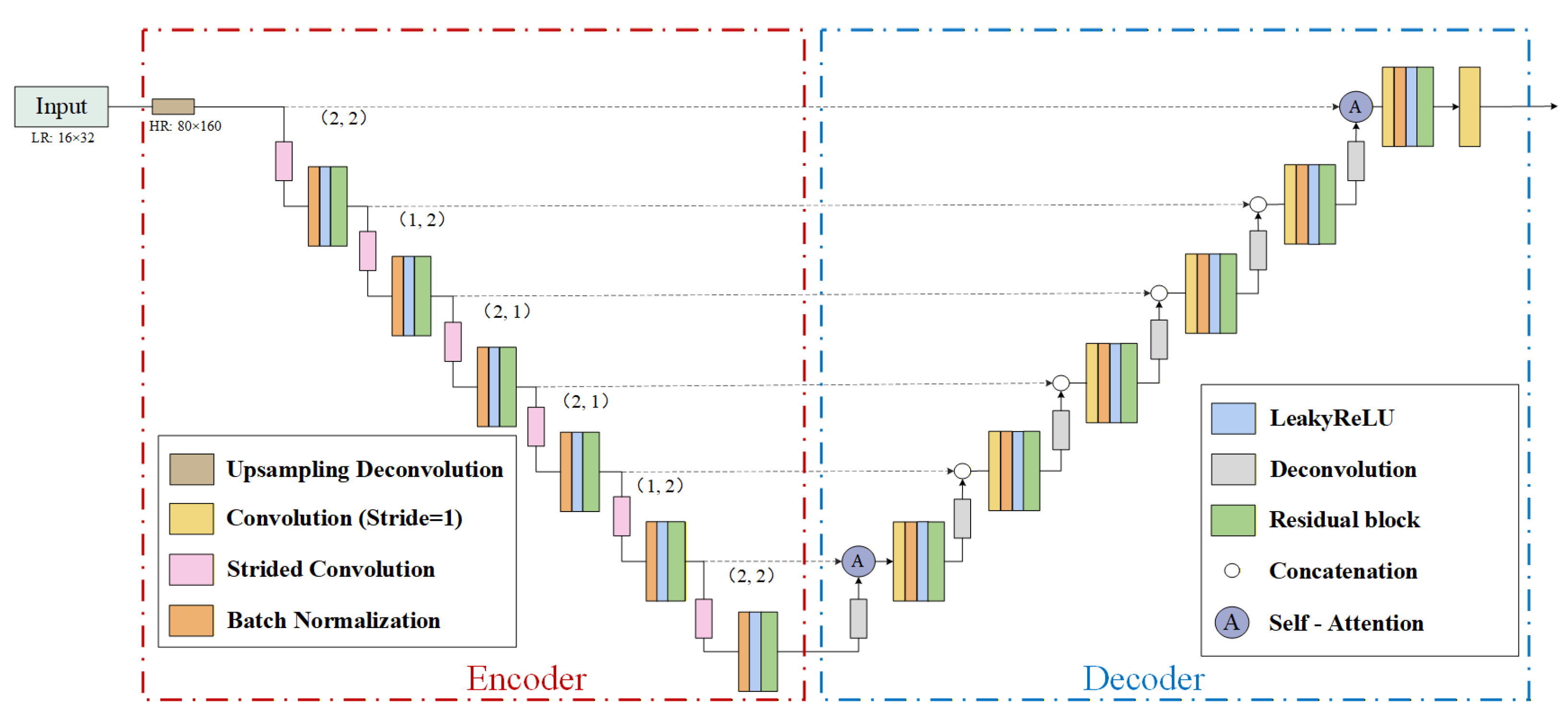
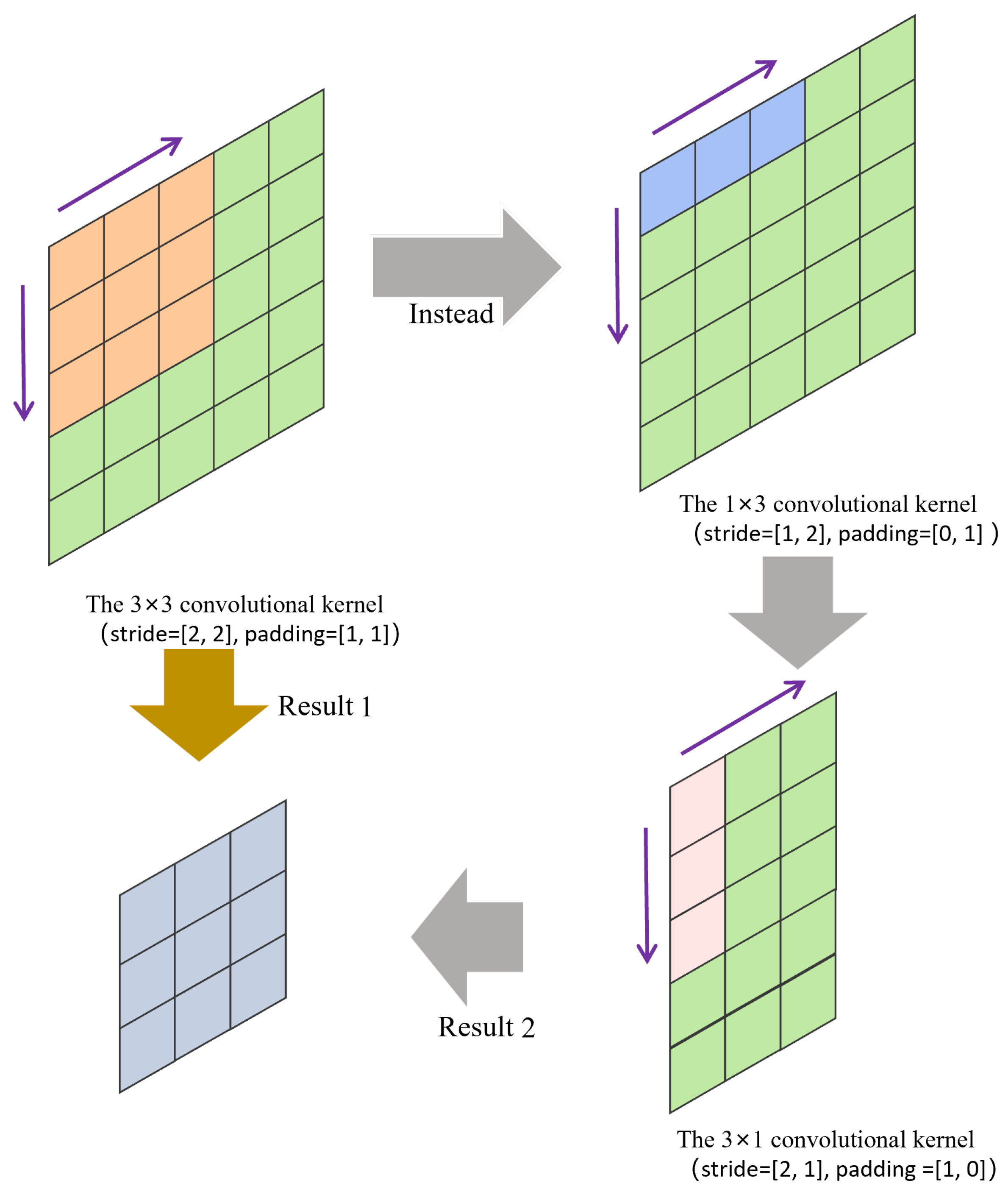
Ronneberger introduced U-Net, which was originally designed for medical image analysis [22]. In our experiments, we employ a U-Net-based encoder–decoder architecture, replacing max pooling with stride convolution for downsampling. Additionally, we decompose the square convolutional kernel into two perpendicular rectangular kernels to deepen the network and capture multi-resolution features. These modifications enhance feature extraction, reduce input signal size in deeper layers, and expand the receptive field, improving model performance. These operations effectively capture detailed features across dimensions, enhancing the estimation accuracy of sea ice internal concentration and dynamic distribution. The revised convolution operation is illustrated in Figure 1.

2.1.2. Residual Network

Due to the utilization of a multi-level symmetrical structure in U-Net, which employs multiple layers of CNN at the encoder–decoder level at the same resolution to enhance SR accuracy, this may give rise to the problem of vanishing or exploding gradients in the network’s multi-level design. To mitigate this, He et al. introduced residual networks, where “residual” refers to the difference between observed and estimated values [23]. In residual learning, shortcut connections perform identity mapping, directly passing inputs from shallow to deep layers without adding parameters, thereby avoiding increased computational complexity. Integrating residual learning into U-Net for SIC downscaling enhances training stability and computational efficiency.

2.1.3. Attention Mechanism

The attention mechanism, inspired by human attention, has become a key technique in deep learning, enhancing the processing of time-series data by allowing neural networks to focus on critical information at different temporal positions [24]. When deriving the attention mechanism, the initial consideration involves three vectors: the query tensor (Q), the key tensor (K), and the value tensor (V). Q represents the information of interest, serving as the input tensor for the attention mechanism. K is employed to measure the extent of correlation between Q and other pieces of information. V denotes the tensor associated with the real information for each Q. The attention mechanism is mathematically formulated as follows:

$$Attention\left(Q,K,V\right)=Softmax\left({\displaystyle \frac{Q·K^T}{\sqrt{d_k}}}\right)·V$$

(1)

where $d_k$ represents the dimensionality of K. Here, each row of the attention scores matrix corresponds to the attention scores between the row i of the query vector Q and every column of the key vector K. To ensure effective weight allocation, the attention scores are typically subjected to a softmax operation, mapping the values in each row to the range [0, 1] and ensuring that the sum of each row’s elements is 1.

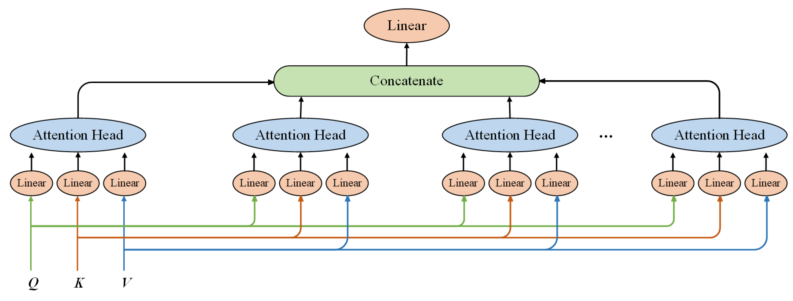
When analyzing a polar SIC spatiotemporal sequence, we employed a specific attention mechanism, the self-attention mechanism, i.e., $Q=K=V$. Specifically, we integrate a parallel self-attention mechanism, multi-head self-attention, into our network. This allows the model to focus on different parts of the input sequence simultaneously, as each attention head learns a unique way of attending to the data. The multi-head mechanism enhances computational efficiency, captures diverse information, and provides a more comprehensive understanding of SIC dynamics [20]. A schematic diagram of this design is shown in Figure 2.

This design enhances the model’s learning capability, allowing it to better adapt to different segments of the input sequence. This is essential for a deeper and more comprehensive understanding and utilization of the data’s potential information.

2.1.4. Deep SARU-Net Architecture

As mentioned above, we employed a CNN-based U-Net as the backbone and integrated an attention mechanism to enhance temporal feature extraction and spatial representation. The temporal attention mechanism enables the model to implicitly capture sea ice drift and dynamic variations, thereby effectively compensating for motion information. Additionally, residual connections were introduced to optimize gradient propagation, facilitating SIC downscaling. We refer to this structure as Deep Self-Attention Residual U-Net (Deep SARU-Net). This design enables a more comprehensive understanding of multi-scale features in the encoding process, providing a foundation for in-depth analysis of sea ice evolution.

In designing Deep SARU-Net, we draw inspiration from research in areas like image SR task and meteorological downscaling. Our approach is based on the classical U-Net, commonly used in biomedical image segmentation, and we experimented with various U-Net variants to enhance SR estimation performance. Additionally, influenced by wind field downscaling research [25], we optimized the model using insights from atmospheric and oceanic SR studies. We find that deepening the architecture by increasing resolution levels led to better training outcomes. However, simply adding more convolutional layers within a single resolution level does not improve estimation quality. Instead, incorporating residual blocks [23] in place of standard convolutions significantly enhanced training performance. The optimal estimation accuracy was achieved when each residual block contained three convolution operations.

To address the limitations of CNNs in capturing temporal features, we incorporated the multi-head self-attention mechanism from the Transformer architecture into our design. This enhanced the capture of temporal features while improving spatial scale representation. During our research, we found that adding attention mechanisms to skip connections at each resolution level increased training time without significantly improving performance. Instead, placing attention mechanisms only at the connections between the encoder and decoder effectively captured temporal features. To focus more on the effectiveness of the model at the target resolution, we introduced an attention mechanism at the first layer of the skip connection, strengthening spatial feature representation. Overall, we applied self-attention mechanisms at the highest (first) and lowest (last) resolution levels, achieving notable improvements in estimation performance with relatively short training times. These insights led to the development of the Deep SARU-Net architecture, as shown in Figure 3.

Deep SARU-Net is a complex CNN built on the U-Net architecture, featuring multiple resolution stages with skip connections and residual blocks. Self-attention mechanisms are incorporated at the first and last resolution stages through skip connections. Initially, channel features are extracted from input data of size 16 × 32, converting them into 16 primary LR feature channels. The LR data is then upsampled using bicubic interpolation to match the target HR data of 80 × 160. The network’s encoder uses continuous convolutions for feature downsampling, while the decoder applies deconvolution operations to enhance resolution, achieving SR estimation of SIC. Batch normalization and the Leaky ReLU activation function are applied throughout. As mentioned in Section 3, the input data is formatted as $C\times lat\times lon$, where C represents the number of days in the input data, and $lon$ and $lat$ denote grid points in the longitude and latitude directions, respectively.

2.2. Loss Functions

To effectively measure the disparity between SR estimations and HR targets, selecting an appropriate loss function is crucial. Initially, we considered using Mean Squared Error (MSE), which evaluates model performance by measuring the squared differences between estimations and ground truth. However, MSE has a drawback due to its squared dependence on data. In cases where large errors exist, this dependence can make the model overly sensitive to significant deviations while being less responsive to smaller errors [25]. This may introduce bias, causing the model to prioritize minimizing large errors at the expense of accurately capturing the overall data distribution. To address this issue, we explored alternative loss functions such as Mean Absolute Error (MAE), Huber loss, and Structural Similarity Index (SSIM) loss. Ultimately, we selected SSIM as our primary loss function. Unlike traditional pixel-wise losses such as MSE or MAE, SSIM incorporates luminance, contrast, and structural information [26], providing a more comprehensive assessment of image similarity. Importantly, SSIM aligns more closely with human perceptual judgments of image quality, which is particularly meaningful for the visual interpretation of sea ice imagery where structural patterns, ice edges, and fine-scale morphology are critical. Given estimated results and ground truth denoted as X and Y, with values at different positions represented by $x\left(i,j\right)$ and $y\left(i,j\right)$, respectively. The luminance term $L(X,Y)$, contrast term $C(X,Y)$ and structure term $S(X,Y)$ in the SSIM equation are expressed as follows:

$$\left\{\begin{array}{c}L(X,Y)={\displaystyle \frac{2{\mu }_x{\mu }_y+C_1}{{\mu }_x^2+{\mu }_y^2+C_1}}\hfill \\ C(X,Y)={\displaystyle \frac{2{\sigma }_x{\sigma }_y+C_2}{{\sigma }_x^2+{\sigma }_y^2+C_2}}\hfill \\ S(X,Y)={\displaystyle \frac{{\sigma }_{xy}+C_3}{{\sigma }_x{\sigma }_y+C_3}}\hfill \end{array}\right.$$

(2)

where ${\mu }_x$ and ${\mu }_y$ are the luminance means of X and Y, ${\sigma }_x$ and ${\sigma }_y$ are the luminance variances of X and Y, ${\sigma }_{xy}$ is the luminance covariance between images X and Y, respectively, and $C_1$, $C_2$, $C_3$ are the constants used to prevent instability caused by a too-small denominator.

Finally, SSIM is computed by combining the products of luminance, contrast, and structural similarities:

$$\mathrm{SSIM}(X,Y)=\left[L(X,Y)\right]\left[C(X,Y)\right]\left[S(X,Y)\right]$$

(3)

2.3. Optimization Strategies

Both Deep SARU-Net and control group models, including LinearCNN [27], SRCNN [28], U-Net [22,29], and Attention U-Net [30,31], are implemented in the PyTorch 2.0 framework. For optimization, we use the ADAM optimizer, which integrates the advantages of stochastic gradient descent (SGD) and RMSprop while incorporating momentum to accelerate convergence [32]. The initial learning rate is $1\times {10}^{-3}$, the termination learning rate is $1\times {10}^{-7}$, the patience value for the learning rate is 30, and the decay factor is 0.1. Furthermore, the weight initialization method for all networks is Kaiming initialization [33], which adjusts the range of weight initialization based on the number of inputs and outputs to make the network more stable during the training process. Additionally, batch normalization [34] is introduced after each convolution operation for all models to enhance convergence speed. To mitigate overfitting and maintain compact model parameters, weight decay (L2 regularization) is applied with a coefficient of $1\times {10}^{-4}$ [35].

For more complex CNN models like U-Net, Attention U-Net, and Deep SARU-Net, a 2D regularization strategy [36] is applied after each residual module with a dropout rate of 0.1. Additionally, an L2 regularization (weight decay) strategy with a decay rate of $1\times {10}^{-5}$ is applied [35]. These techniques collectively enhance model stability and generalization, accelerate convergence, and reduce the risk of overfitting.

3. Dataset

Our study utilized satellite remote sensing Arctic SIC data, including both LR (0.5° × 0.5°) and HR (0.1° × 0.1°) datasets for model training and evaluation. These datasets were sourced from the Copernicus Marine Environment Monitoring Service (CMEMS) global ocean OSTIA sea surface temperature and sea ice analysis [37,38,39]. Below, we provide an overview of the domain description and the data resolution.

3.1. Domain Description

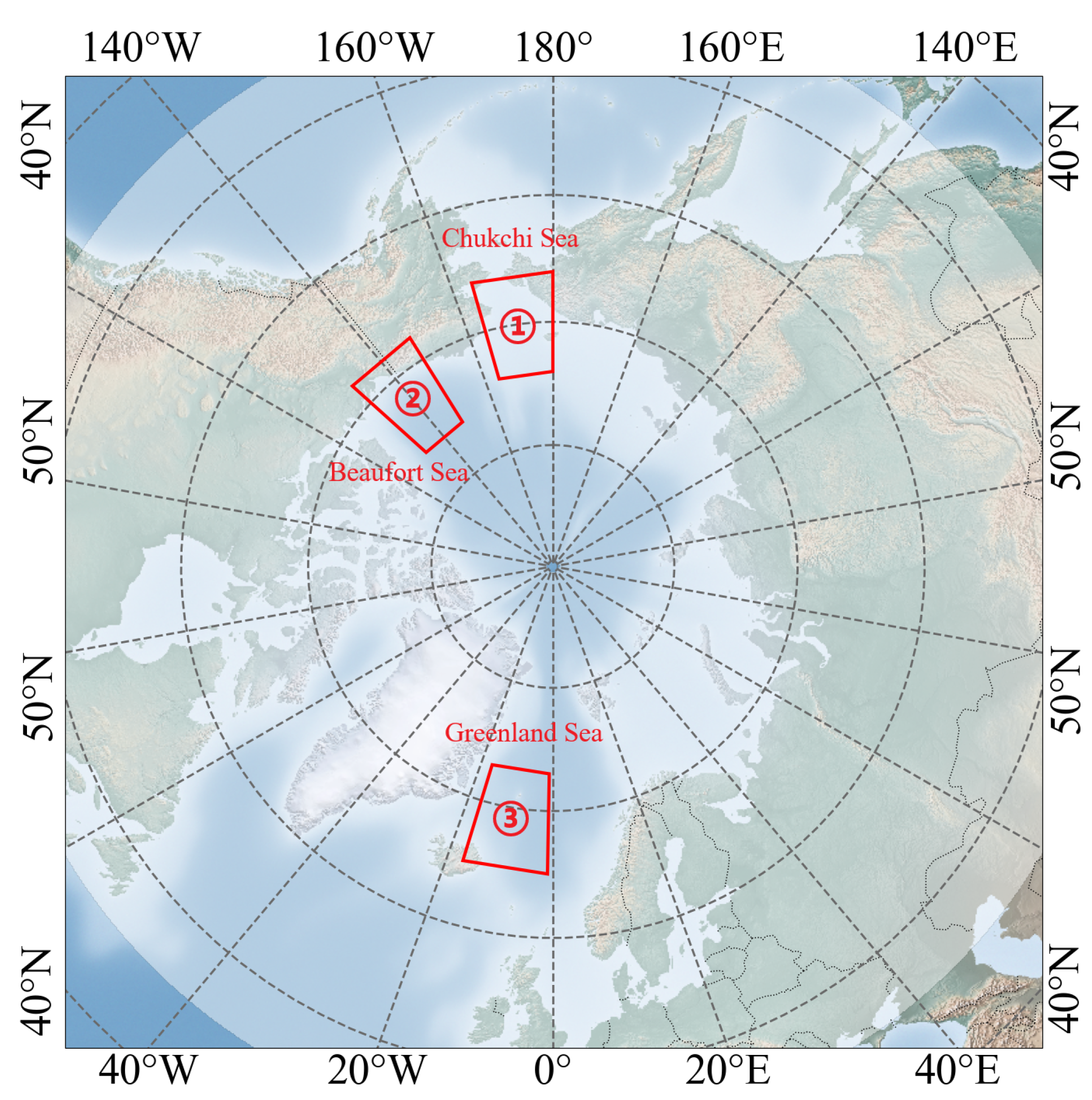
The primary study domain of this research is the Chukchi Sea (66°N–74°N, 180°W–164°W), located between northwestern Alaska (USA) and the Chukotka Autonomous Okrug (Russia). It is bounded by Wrangel Island to the west, the Beaufort Sea to the east, and the Bering Strait to the south, which connects it to the Bering Sea and the Pacific Ocean. The Chukchi Sea plays a vital role in global climate regulation and serves as a key monitoring region for Arctic climate change. The observed processes of sea ice melt and formation in this region effectively reflect variations in temperature and ocean circulation. Therefore, conducting HR research on SIC in the Chukchi Sea is crucial for understanding sea ice dynamics, evaluating the feasibility of Arctic navigation, and supporting global climate monitoring efforts. In addition, to assess the generalization capability of the proposed model across different marine regions, we selected two representative areas, the Beaufort Sea (68°N–76°N, 148°W–132°W) and the Greenland Sea (65°N–73°N, 17°W–1°W), for validation experiments. All regions involved in the study are illustrated in Figure 4.

3.2. LR and HR Data

As LR input and HR target data for our models, we utilized global ocean OSTIA sea surface temperature and sea ice remote sensing products from CMEMS, sourced from the UK Met Office. This dataset integrates in situ and satellite observations from infrared and microwave radiometers, providing key variables such as sea surface temperature (SST), SIC, and land-water interface data. The dataset has a maximum spatial resolution of 0.05° × 0.05° and a maximum daily temporal resolution.

This study is designed as a verification experiment to evaluate the SR estimation capability of the proposed model. Considering both the spatial variability of Arctic sea ice and the computational complexity of the network, we set the LR data resolution to 0.5° × 0.5° (16 × 32 grids) and the HR resolution to 0.1° × 0.1° (80 × 160 grids), both derived from the original 0.05° × 0.05° dataset using kriging interpolation. The choice of spatial resolutions for the LR and HR datasets reflects the verification-oriented nature of this study: our goal is to assess the SIC SR estimation performance of Deep SARU-Net while balancing the characteristic spatial scales of Arctic sea ice and computational efficiency. Both LR and HR datasets maintain a daily temporal resolution. The full dataset spans the period from 1 January 2018 to 31 December 2022, with February 29 removed in leap years.

Table 1. Description of the datasets used in the study.

Attribute	Details
Product	OSTIA Sea Surface Temperature and Sea Ice Analysis
Temporal range	1 January 2018–31 December 2022
Spatial range	66°N–74°N, 180°–164°W
Temporal resolution	Daily average
Spatial resolution	1/2° grid (LR)
	1/10° grid (HR)
Dataset partitioning	2018–2020 (Train set)
	2021 (Validation set)
	2022 (Test set)

summarizes the dataset composition. Specifically, the first three years (2018–2020) are used for model training (1095 days), the year 2021 serves as the validation set (365 days) for updating model parameters, and the year 2022 is reserved as the test set (365 days) for final model evaluation.

In addition, we employed the Arctic Ocean—High Resolution Sea Ice Information L4 dataset, which is derived from Sentinel-1 SAR imagery and provides HR, observation-based sea ice information with a native spatial resolution of 1 km × 1 km. This dataset was selected to further evaluate the model’s generalization capability across different types of in situ observation products. For consistency with the other datasets used in our experiments, we applied cubic interpolation based on kriging to resample the L4 data to the same spatial resolution.

4. Experimental Setup and Results

In this section, we will focus on the SR estimation of SIC in polar regions. The experimental data, model hyperparameters, and input–output formats have been discussed earlier and will not be repeated here. Hardware parameters are provided in

Table 2. Description of the hardware parameters in the study.

Component	Model
CPU	Intel(R) Core(TM) i9-10900K
GPU	Nvidia GeForce RTX 3080
Memory	64 GB DDR4 (3200 MHz)
Storage	SSD 2 TB NVMe M.2

below. The section is structured into subsections, where we will elaborate on the evaluation indicators, experimental design, and relevant analyses.

4.1. Evaluation Indicators

Building on relevant research in ocean estimation and image SR tasks, various evaluation metrics can be used to assess model performance in SIC SR estimation from multiple perspectives. In this study, we focus on four key evaluation indicators Root Mean Square Error (RMSE), Pearson Correlation Coefficient (PCC, r), Peak Signal-to-Noise Ratio (PSNR), and SSIM to comprehensively assess model performance. Since a detailed explanation of SSIM has already been provided in Section 2.2 (Loss functions), we will not elaborate on it further here.

The RMSE is a widely used metric for evaluating the average magnitude of errors between reconstructed values and ground truth. In the context of SR estimation, it provides a solid assessment of model performance by quantifying the difference between the model’s SR estimations and the HR ground truth. The equation for RMSE is expressed as follows:

$$RMSE=\sqrt{{\displaystyle \frac{1}{n}}\sum _{i=1}^n{(G_i-P_i)}^2}$$

(4)

where $G_i$ denotes the HR ground truth and $P_i$ denotes the SR estimations at grid i, i is the index of the grid order, and n denotes the total number of grids.

RMSE primarily focuses on assessing the overall deviation between ground truth and estimations. However, r is more inclined towards evaluating whether the model can accurately capture the linear relationships between variables, providing a more detailed understanding of model performance. Specifically, the calculation of r can be expressed as follows:

$$r={\displaystyle \frac{{\sum }_{i=1}^n(P_i-\overline{P})(G_i-\overline{G})}{\sqrt{{\sum }_{i=1}^n{(P_i-\overline{P})}^2{\sum }_{i=1}^n{(G_i-\overline{G})}^2}}}$$

(5)

where $\overline{P}$ denotes the average of P and $\overline{G}$ denotes the average of G.

Inspired by image SR research, we introduce two metrics: PSNR and SSIM, to evaluate the model’s performance. These metrics focus on perceptual image quality, offering a more comprehensive assessment, especially for tasks like image SR.

PSNR is a widely used metric in image and video processing to assess the effectiveness of compression techniques [40]. It measures the quality of compressed images or videos by evaluating information preservation during compression. The formula for PSNR is:

$$PSNR=10·{log}_{10}\left({\displaystyle \frac{MA{X}^2}{MSE}}\right)=20·{log}_{10}\left({\displaystyle \frac{MAX}{RMSE}}\right)$$

(6)

where MAX is the maximum possible value for a pixel in the image (for floating-point data, its maximum pixel value is 1).

4.2. Experimental Design

In the experimental design, six benchmark models were selected for comparison. These include the traditional method of bilinear interpolation; two models based on simple CNN architectures, namely LinearCNN and SRCNN; and three models built on more complex CNN architectures, namely U-Net, Attention U-Net, and PMDRnet. All of these approaches represent widely adopted and classical baselines in SR tasks.

4.2.1. Analysis of the Impact of Input Days on Model Performance

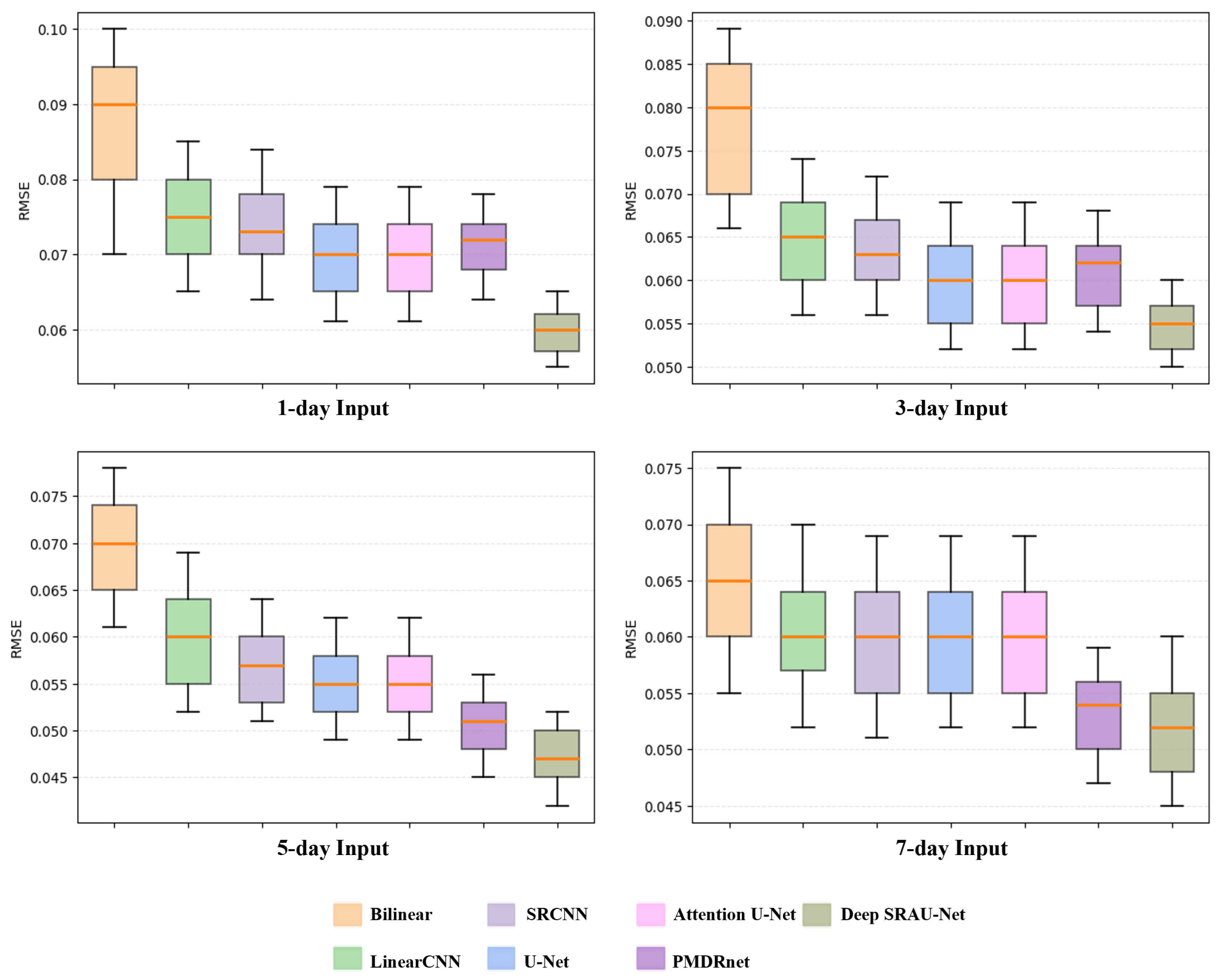
To establish a scientifically sound experimental workflow, we first conducted an exploratory analysis of the input sequence length to assess its impact on model performance. This step is essential for understanding the model’s sensitivity to temporal information and identifying the optimal input configuration, which in turn helps enhance the effectiveness and efficiency of subsequent SR reconstruction. Specifically, we evaluated the performance of SR estimation under different input durations (1 day, 3 days, 5 days, and 7 days). This comparison aims to explore how various network architectures respond to extended temporal inputs. Figure 5 presents the impact of different input sequence lengths on model performance.

Figure 5 shows the RMSE distribution for various models with different input sequence lengths. Generally, the RMSE decreases progressively as the input sequence length increases from 1 to 5 days, suggesting that model performance improves with more input days, provided there is no overfitting on the validation set. It is noteworthy that deep CNNs, particularly U-Net, Attention U-Net, PMDRnet, and Deep SARU-Net, exhibit more concentrated RMSE distributions. Among them, Deep SARU-Net demonstrates the tightest distribution, followed by PMDRnet, while U-Net and Attention U-Net show comparable performance. This indicates that Deep SARU-Net achieves the least data fluctuation, the most stable distribution, and the best overall performance.

However, as the input sequence length increases, the risk of model overfitting also rises. In our experiments, when the input sequence length reached 7 days, most networks showed signs of overfitting, resulting in a noticeable decline in reconstructive performance. The RMSE size and tightness exhibit fluctuations when the input number of days is 7, confirming the overfitting issue. This trend is understandable: a longer input sequence provides the model with more temporal context, which helps capture the evolving patterns of SIC. While additional input days offer valuable context for learning sea ice changes, an excess of input information can lead to overfitting, as the model might start learning noise rather than generalizable features.

To mitigate overfitting and improve model performance, we selected a 5-day input sequence for the subsequent experiments. Under this configuration, Deep SARU-Net achieved a notable reduction in average RMSE, dropping to 0.0449. Furthermore, its correlation coefficient (r) increased to 0.9962, PSNR reached 32.03, and SSIM rose to 0.9744, demonstrating significant improvements across all metrics.

4.2.2. Performance of the Self-Attention Mechanism

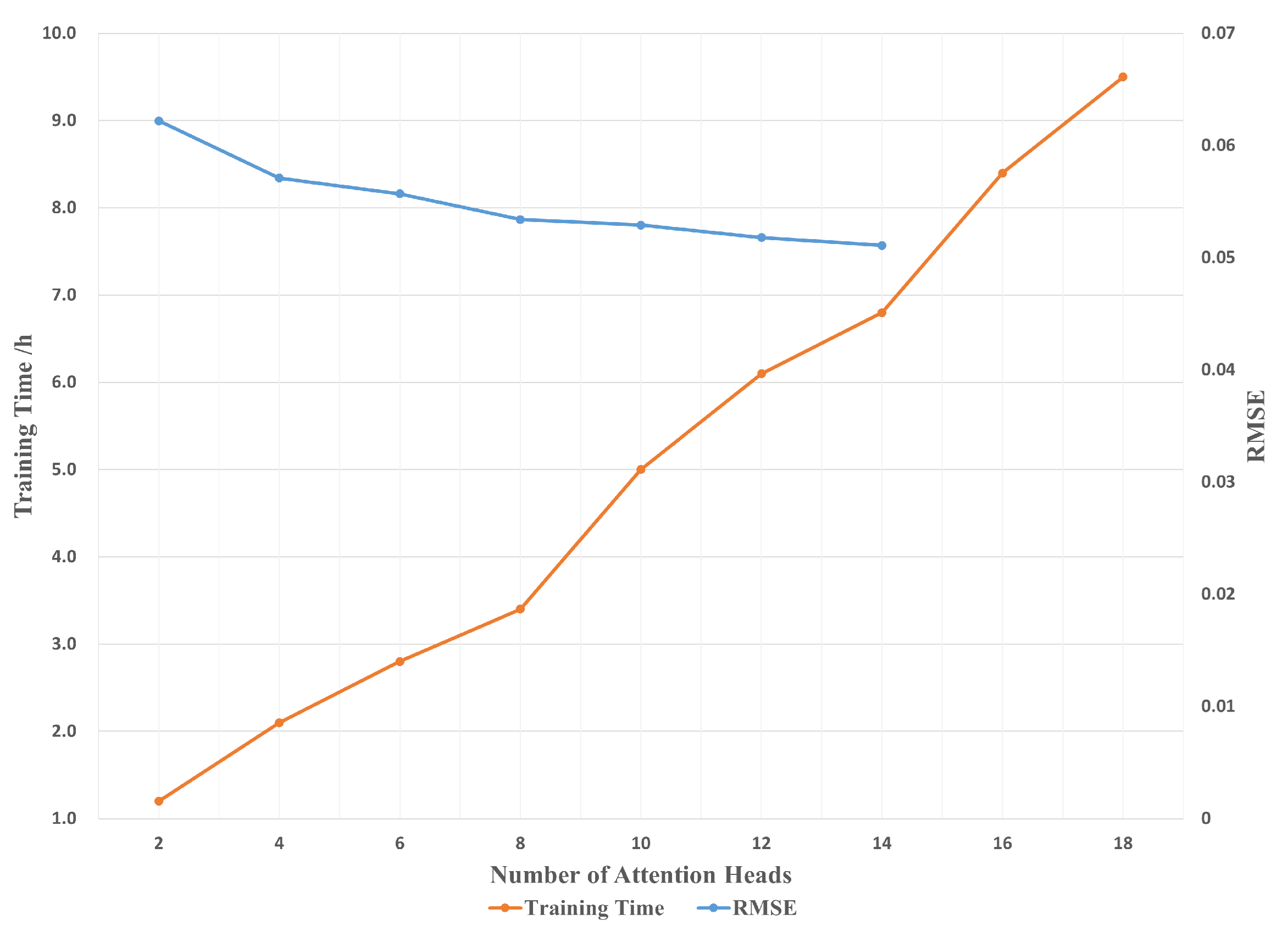
In the previous section, we identified 5 days as the optimal input sequence length. In this section, we further investigate the role and effectiveness of the self-attention mechanism embedded in the model architecture. Deep SARU-Net incorporates a multi-head self-attention mechanism, where each head captures different spatial and temporal feature correlations, thereby enhancing the model’s ability to learn complex dependencies. However, increasing the number of attention heads introduces notable computational and memory overhead, as each head involves intensive matrix operations. Moreover, an excessive number of heads may lead to overfitting—particularly when training data is limited—because the dimensionality of features processed by each head decreases, potentially causing information loss. Therefore, selecting an appropriate number of attention heads is critical for balancing computational efficiency, model capacity, and generalization performance. Based on a series of optimization trials, we set the number of attention heads to 8. The experimental results supporting this choice are presented in Figure 6.

The curves in the chart clearly demonstrate that increasing the number of attention heads leads to a longer total training duration, reflecting higher computational resource demands. In terms of RMSE, which measures model accuracy, a lower value indicates a better fit to the observed data. As the number of attention heads increases to 8, RMSE consistently decreases, signifying improved model performance. However, beyond 8 attention heads, the reduction in RMSE plateaus, indicating diminishing returns on performance relative to the rising computational cost.

Additionally, when the number of attention heads exceeds 14, the model begins to exhibit signs of over-fitting, suggesting that it may be capturing noise rather than true underlying patterns in the data. A comprehensive analysis indicates that the optimal balance between low RMSE and reasonable training time is achieved at 8 attention heads. This configuration ensures an effective trade-off between computational efficiency and model performance, maintaining strong spatiotemporal feature capture without excessive over-fitting. Ultimately, we selected an input sequence length of 5 days and set the number of attention heads to 8 as the unified configuration for all subsequent experiments.

4.2.3. Run-Time Performance and Memory Requirements

In this study, we focus on a comprehensive analysis of several key aspects during the model execution process, including trainable parameters, memory consumption, total training time, and single SR estimation time. To ensure scientific validity and reliability, we implemented rigorous experimental designs and method controls.

To ensure consistency and comparability, we process data in batches of 40 to 60 samples, depending on memory availability. This experiment focuses on single-channel input and output, specifically targeting SR estimation for single-day data. When calculating trainable parameters, we account for the increased computational complexity as the network deepens. We consider the entire training cycle, including SR estimation, loss computation, and parameter optimization, to comprehensively evaluate model performance. For a single SR estimation time, we use the average inference time on the validation set as a representative measure.

To minimize errors caused by hardware response time and process delays, we conducted five experimental measurements for each model and averaged the results. This includes the total training duration (500 epochs, 4-year training set) and the total SR estimation time (1-year validation set). The single-step estimation time is calculated as the ratio of the total estimation time to the number of validation set inputs. Detailed metrics from different experimental runs for each model are summarized in

Table 3. Run-time performance statistics for LinearCNN, SRCNN, U-Net, Attention U-Net, and Deep SARU-Net.

Model	TP	MEM	TR	PS
LinearCNN	148.5	0.6	1.1	1.2
SRCNN	517.9	2.5	1.1	2.9
U-Net	1370.1	7.2	4.2	7.9
Attention U-Net	1970.4	11.9	5.1	10.2
PMDRnet	4841.6	22.1	13.5	31.6
Deep SARU-Net	1207.2	6.1	3.4	7.3

Notes: The first column of the table identifies the models compared in this experiment. The second column represents the number of trainable parameters (TP) in thousands (k). The third column indicates the memory consumption required to store the model (MEM) in megabytes (MB). The fourth column records the total training procedure duration (TR) in hours (h). The last column presents the single estimation procedure step (PS) in milliseconds (ms).

.

Experimental results demonstrate that increasing model complexity leads to a substantial rise in computational costs. Compared to the simpler LinearCNN and SRCNN models, deep CNNs based on the U-Net architecture show a significant escalation in both parameter scale and computational time. The Attention U-Net, due to the incorporation of the attention mechanism, also exhibits a slight increase in parameters and computation time compared to the standard U-Net. PMDRnet, with its parallel multi-branch design, registers the highest parameter count and total training duration. To address this challenge, our proposed Deep SARU-Net adopts a sequential convolutional design and incorporates self-attention mechanisms solely in the skip connections at the highest and lowest resolution levels, thereby achieving an effective reduction in the number of trainable parameters. Compared to U-Net, Attention U-Net, and PMDRnet, Deep SARU-Net achieves a significant reduction in parameters by 11.9%, 38.8%, and 75.1%, respectively. Furthermore, by strategically introducing residual blocks, we successfully enhance the predictive performance without inflating the parameter count, making Deep SARU-Net more advantageous than conventional U-Net, and demonstrating marked improvements in memory consumption, total training procedure duration, and single estimation procedure step.

Although Deep SARU-Net contains fewer parameters than the other two deep networks, its reconstructive performance has not yet been fully validated. Therefore, in the next section, we analyze the downscaling performance of different SR models.

4.2.4. Performance Evaluation of SR Estimation Models

This study aims to evaluate the performance of Deep SARU-Net in SIC SR estimation and compare it with six baseline models. All experiments are conducted under a unified configuration of 5-day input and 1-day output, with model performance assessed on the validation dataset using RMSE, correlation coefficient (r), PSNR, and SSIM. The detailed results are presented in

Table 4. Comparison of model performance for single-day SIC SR estimation across different network architectures (5-day input).

Metric	Bilinear	LinearCNN	SRCNN	U-Net	Attention U-Net	PMDRnet	Deep SARU-Net
RMSE	0.1101	0.0943	0.0758	0.0685	0.0642	0.0532	0.0449
r	0.9487	0.9589	0.9668	0.9769	0.9830	0.9928	0.9962
PSNR	21.10	24.12	26.07	28.45	29.21	29.47	32.03
SSIM	0.8612	0.9018	0.9199	0.9558	0.9598	0.9584	0.9744

.

The table provides a comparative analysis of different models for single-day SIC SR estimation. Among the six methods, bilinear interpolation exhibits the weakest performance, with the highest overall error and the lowest PSNR and SSIM values, indicating poor spatial detail enhancement. LinearCNN and SRCNN, as basic CNN models, improve spatial detail representation through convolution operations, outperforming bilinear interpolation. However, both employ uniform linear convolution kernels across the entire sea domain, producing general estimates while limiting precision, particularly for complex regions like sea ice edges and sea-land interfaces. As a result, their SR performance remains suboptimal in capturing fine-scale SIC variations.

The remaining four methods, U-Net, Attention U-Net, PMDRnet, and Deep SARU-Net, are more complex deep neural networks and overall demonstrate better performance. Standard U-Net and Attention U-Net achieve RMSE values of 0.0685 and 0.0642 on the validation set, respectively, but still fall short compared to the other two models. PMDRnet attains an RMSE of 0.0532, second only to Deep SARU-Net. This indicates that increasing the number of trainable parameters and incorporating attention mechanisms can indeed improve performance. However, higher model complexity also introduces the risk of overfitting. Even with L2 regularization and dropout applied, signs of overfitting remain observable. In addition, although PMDRnet achieves relatively strong performance in terms of RMSE, its SSIM is slightly lower than that of Attention U-Net. On the one hand, this is partly attributed to overfitting; on the other hand, it is related to the mismatch between data characteristics and model design. The original PMDRnet was specifically developed for processing AMSR2 passive microwave remote sensing images, whereas this study employs multi-source satellite remote sensing products that have been fused and regridded. These data differ substantially from raw AMSR2 imagery in terms of spatial resolution, noise properties, and statistical distribution, which reduces PMDRnet’s effectiveness in SR reconstruction.

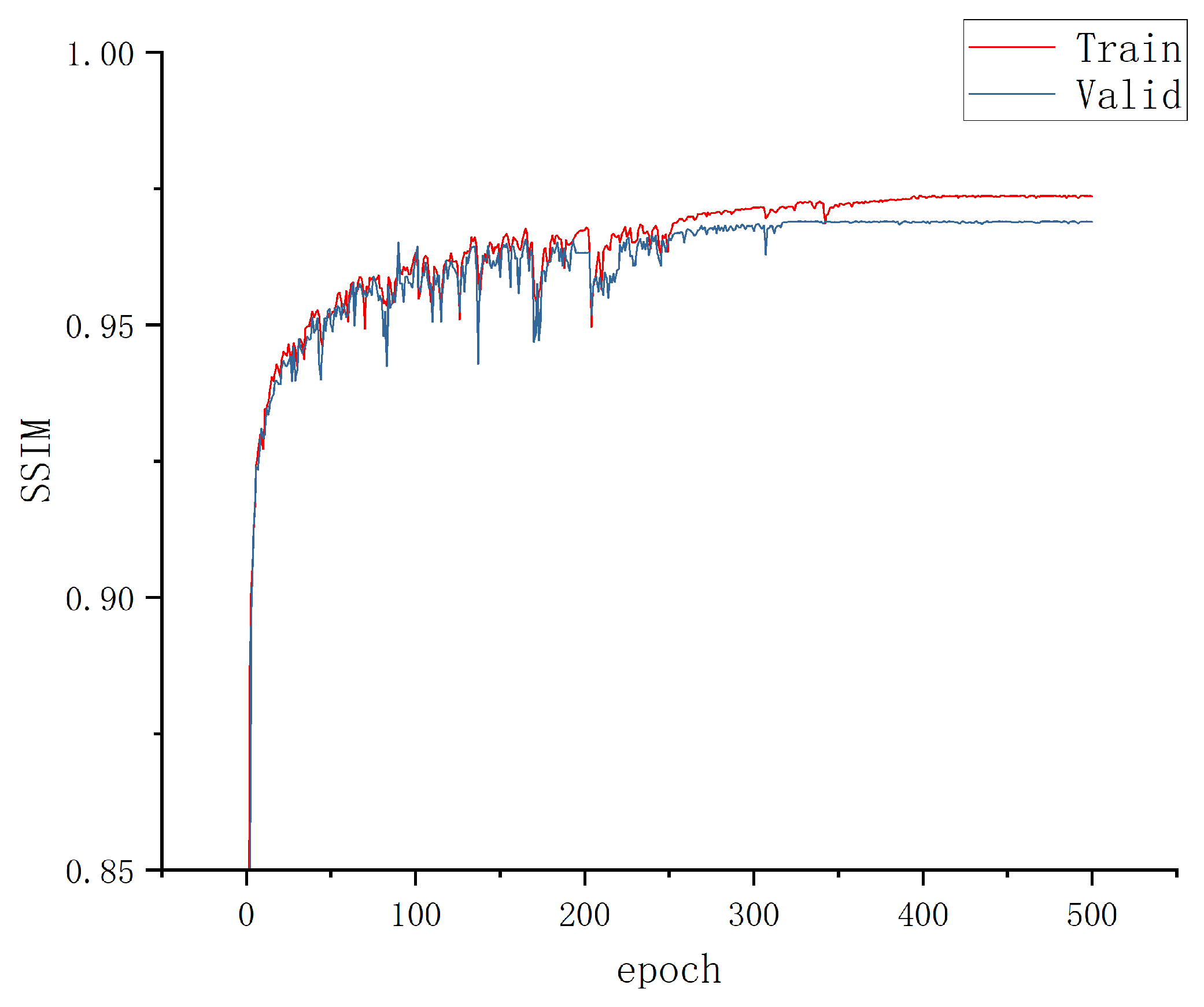
Deep SARU-Net effectively mitigates overfitting by redesigning the encoder–decoder architecture and optimizing the integration of attention mechanisms with residual connections. This optimization not only reduces the number of trainable parameters and simplifies the network structure but also preserves strong generalization capability. Experimental results demonstrate that the model achieves the best performance in SIC SR estimation, with an RMSE of 0.0449, correlation coefficient (r) of 0.9962, PSNR of 32.03 dB, and SSIM of 0.9744. Compared to bilinear interpolation, RMSE is reduced by 59.29%, r is increased by 5.00%, PSNR improves by 51.77%, and SSIM rises by 13.15%. Compared with the next-best model, PMDRnet, the RMSE is reduced by 15.60%, the correlation coefficient r increases by 0.34%, the PSNR improves by 8.69%, and the SSIM rises by 1.67%. These improvements clearly highlight the model’s remarkable ability to enhance image quality and spatial correlation. Figure 7 presents the training and validation loss curves (SSIM and RMSE) of Deep SARU-Net, showing no signs of overfitting.

4.2.5. Spatial Distribution of Estimation Results

The analysis of the above experimental results primarily relies on data-based metrics. However, these metrics provide limited insight and may not intuitively or comprehensively present the SIC SR estimation outcomes and their spatial error distributions. In this section, we conduct a more detailed analysis from a spatial distribution perspective, focusing on critical areas such as the seacoast, sea ice edges, and the interior of sea ice. By comparing HR ground truth with the SR estimations produced by the model, we aim to provide a more intuitive understanding of the model’s performance in key locations, facilitating a deeper evaluation of its capabilities.

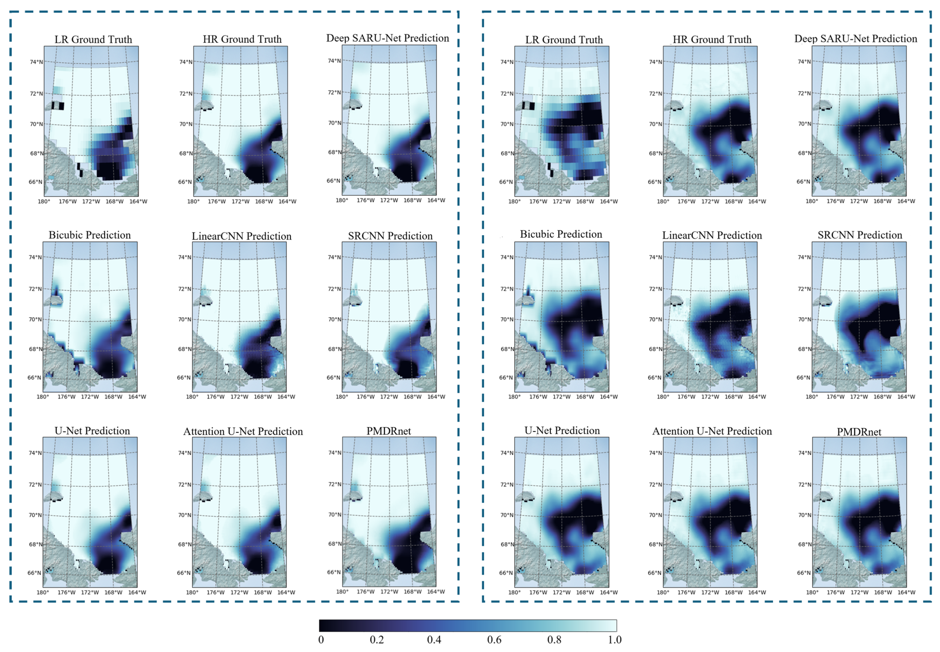
As mentioned earlier, the input sequence length is set to 5 days, using LR SIC data from T-5 to T-1 days to reconstruct the SR result for the Tth day. Among the various models considered, we selected the group that performed best in the SSIM evaluation. The spatial distribution of the SIC SR estimation results is illustrated in Figure 8.

Figure 8 shows the SIC SR estimation results for 1 June 2022 (first half of the year) and 28 December 2022 (second half of the year), respectively. In the SIC LR data, the sea ice distribution near the ice edge and coastal areas is largely inaccurate, especially in the southeastern part of the Chukchi Sea, where the floating ice appears blurry. Compared to the LR data, all seven models successfully perform SIC SR estimation, providing more accurate results for the detailed distribution of sea ice at the ice edge and within the sea ice.

Taking the left panel as an example, it is evident that bilinear interpolation produces blurred boundaries near the coastline. Within the ice edge and interior sea ice regions, the estimated results appear overly smoothed, lacking small-scale variations. In addition, checkerboard-like artifacts can be observed along the coast and in the southeastern Chukchi Sea. These artifacts are likely caused by differences in spatial resolution and grid structure between the LR and HR datasets, as well as the bilinear interpolation method applied during visualization.

LinearCNN and SRCNN, as relatively simple CNN-based models, improve the clarity of land–sea boundaries to some extent. However, significant inaccuracies remain at the sea ice edge. While LinearCNN performs better than SRCNN in certain aspects, it also introduces more pronounced artifacts that undermine reliability. In contrast, more complex deep CNN models—U-Net, Attention U-Net, PMDRnet, and Deep SARU-Net—achieve sharper boundaries and higher spatial SR estimation accuracy. Although Attention U-Net incorporates the CBAM attention mechanism, its performance improvement over U-Net remains limited. This limitation is primarily due to its large number of trainable parameters, which causes parameter redundancy, and the fact that its attention mechanism focuses only on spatial and channel features without effectively capturing more complex contextual dependencies. PMDRnet, despite employing temporal attention to integrate information from different time steps, still shows suboptimal reconstruction performance in the interior ice regions.

Overall, Deep SARU-Net demonstrates the most superior performance. By redesigning the network architecture and integrating residual networks with multi-head self-attention mechanisms, its performance is significantly enhanced. The residual network facilitates more efficient gradient propagation and accelerates training, while the multi-head self-attention mechanism enables the model to capture complex dependencies among sequence elements. As a result, Deep SARU-Net exhibits outstanding SR estimation capability in mixed ice–water regions, with superior detail preservation. For the right panel of Figure 8, we can conduct a similar analysis.

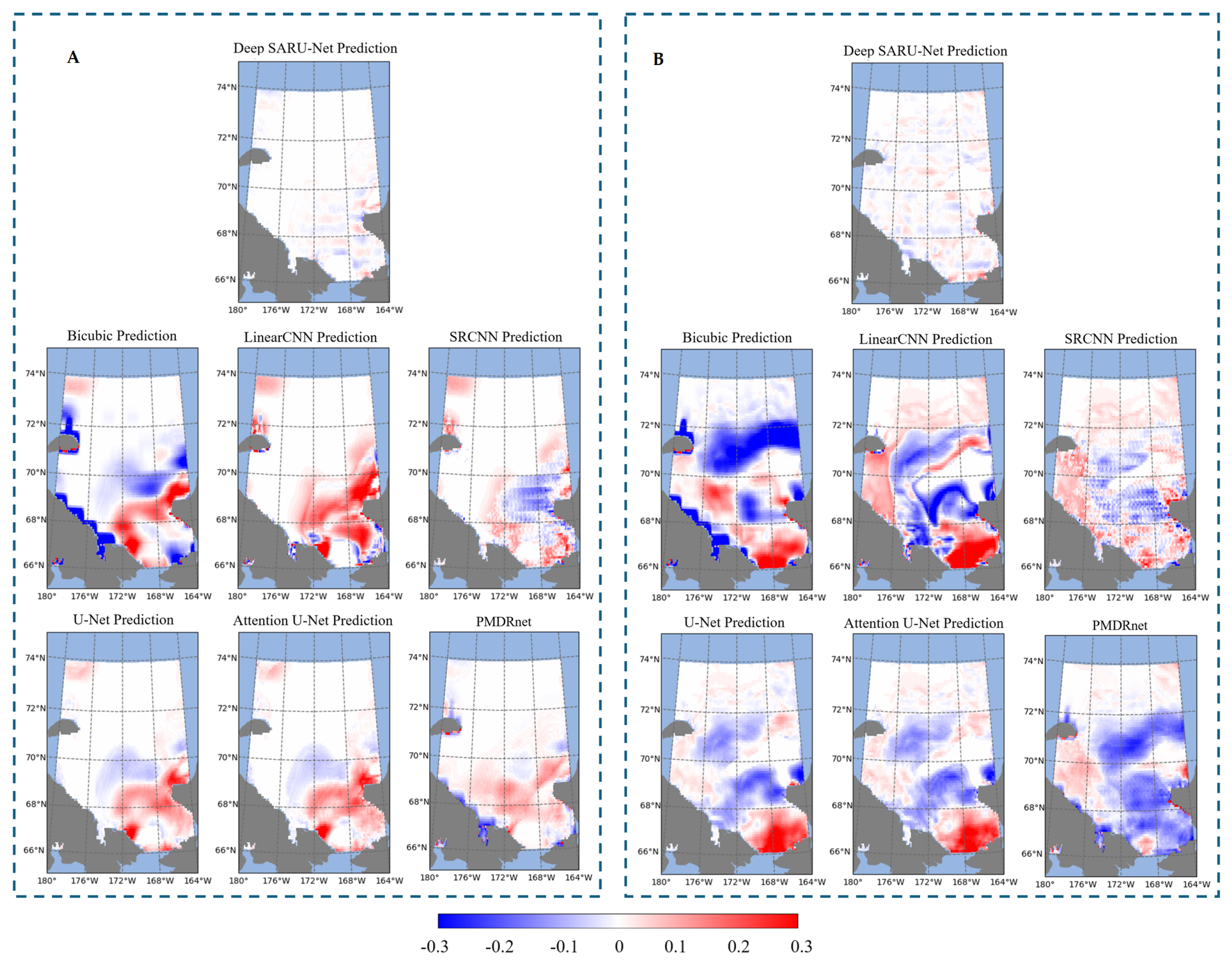
The SIC SR estimation results fall short in clearly, intuitively, and concisely expressing the small-scale distribution and magnitude of errors for various methods. Therefore, we computed the discrepancies between the SR estimated values and the HR ground truth, referred to as residuals, to more accurately unveil the model’s performance. Figure 9 contrasts the residuals of different SR estimation models, vividly illustrating the disparities between the estimated outcomes and HR ground truth.

In the SR estimation results for 1 June 2022 (left panel), the bilinear interpolation model exhibits substantial residuals across large sea areas, underscoring its limitations in capturing the complex spatial patterns of sea ice distribution. Although LinearCNN and SRCNN, as convolutional neural networks, outperform interpolation overall, they still produce considerable residuals in dynamically complex regions such as coastlines and sea ice edges. This indicates that simpler models with fewer parameters struggle to fully represent the intricacies of sea ice dynamics. In contrast, U-Net and Attention U-Net demonstrate better generalization, with Attention U-Net showing a slight improvement in reducing residuals in critical areas. PMDRnet achieves smaller overall errors compared to Attention U-Net, with residuals generally constrained within the range of [−0.15, 0.15], though notable deviations remain in coastal regions. Most notably, Deep SARU-Net achieves the smallest residuals overall, with error values largely confined to [−0.1, 0.1], particularly excelling along sea ice edges and coastlines. These findings suggest that the redesigned architecture of Deep SARU-Net enables it to more effectively capture the complex spatiotemporal dynamics of sea ice, resulting in more accurate estimations.

In the SR estimation results for 28 December 2022 (right panel), the residual distributions across models remain consistent with the earlier findings. A comparison between the left and right panels reveals that winter residuals are generally larger than those in summer. This can largely be attributed to the prolonged “triple-dip” La Niña event since 2020, which lowered Pacific SSTs and influenced Arctic sea ice dynamics, including those in the Chukchi Sea. La Niña typically strengthens Arctic oscillations, intensifies westerlies, and reduces sea ice extent. In summer, cooler temperatures may stabilize sea ice cover, leading to more accurate estimations; in contrast, winter introduces greater variability in sea ice due to shifts in atmospheric circulation, complicating reconstructions. Despite these challenges, Deep SARU-Net successfully constrains residuals within [−0.06, 0.06], underscoring its robust SR performance.

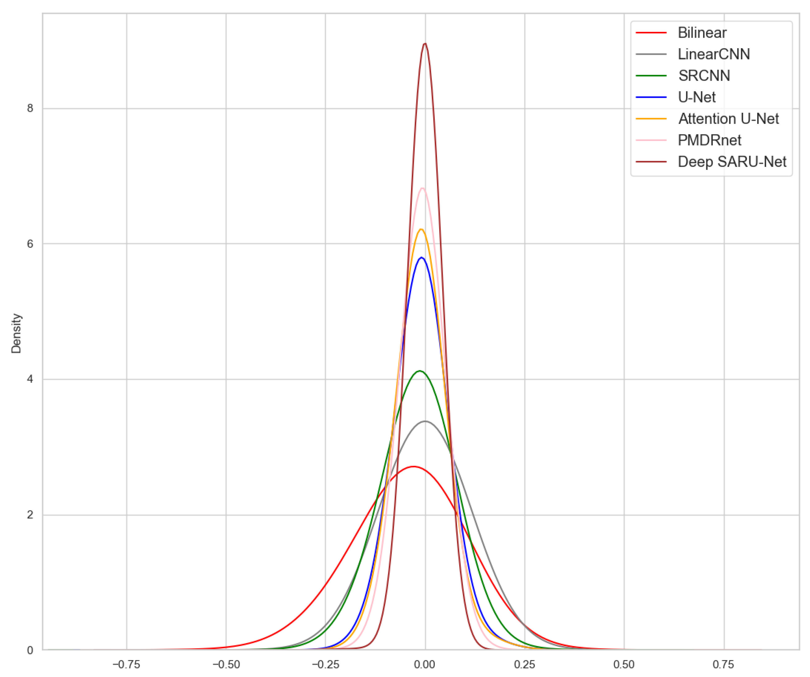
To evaluate the residual distribution across the entire validation set, we applied Gaussian kernel density estimation, a non-parametric method widely used in statistical analysis. This experiment analyzed SIC SR estimations over 365 days (80 × 160 grid points per day, totaling over 4.6 million points). Using kernel density estimation, we statistically examined the residual distribution of different methods, as shown in Figure 10. This figure provides a comprehensive visualization of residual distributions across the validation set.

Figure 10 illustrates the distinct residual distribution patterns across different methods. Bilinear interpolation exhibits the widest range and lowest kurtosis, with residuals primarily spanning [−0.5, 0.3], indicating lower accuracy. In contrast, LinearCNN and SRCNN produce more compact distributions with higher kurtosis, suggesting that CNNs can effectively capture spatiotemporal features for finer SR estimation. Moreover, the U-Net–based models demonstrate superior performance, with residuals becoming more concentrated and kurtosis substantially increased. The symmetric structure and skip connections of U-Net facilitate efficient feature integration, enhancing its capability for spatiotemporal SR tasks, while Attention U-Net further improves residual concentration through its attention mechanism. PMDRnet achieves a peak height second only to Deep SARU-Net, though the difference from Attention U-Net is marginal. Deep SARU-Net delivers the best overall performance, with the smallest residual variance and the most compact distribution, primarily confined to [−0.1, 0.1]. Its near-zero mean residuals and approximately random distribution indicate higher reconstructive accuracy.

4.2.6. Ablation Experiments on Different Modules

Following the previous experiments that validated the strong performance of Deep SARU-Net in Arctic SIC SR estimation, we conducted a series of ablation studies to systematically assess the effectiveness of each proposed architectural enhancement. By progressively removing key modules from the full model, we quantitatively evaluated their individual contributions to SR performance. This section focuses on three components: orthogonal rectangular convolutional kernels, residual blocks, and multi-head self-attention mechanisms.

To ensure fairness, all compared models were trained with the same dataset, loss functions, and optimization strategies, using a consistent input sequence length of 5 days and 8 attention heads (unless the attention mechanism was removed). Four model variants were constructed for comparison: Baseline Model: A standard U-Net architecture with all enhancements removed; Model 1: Adds orthogonal rectangular convolutional kernels to replace max pooling layers; Model 2: Builds on Model 1 by incorporating residual connections; Deep SARU-Net: Adds multi-head self-attention mechanisms to form the full model.

Table 5. Ablation study: Impact of different module combinations on model performance.

Model	RMSE	r	PSNR	SSIM
Baseline Model	0.0736	0.9835	29.47	0.9572
Model 1	0.0619	0.9901	30.62	0.9647
Model 2	0.0527	0.9939	31.28	0.9689
Deep SARU-Net	0.0449	0.9962	32.03	0.9744

presents the performance metrics of each model on the validation set. The results show that each module contributes significantly to performance improvement, with accuracy and stability increasing as more enhancements are included. Compared to the baseline, adding orthogonal convolutions reduced RMSE from 0.0736 to 0.0619 and increased PSNR by approximately 1.15 dB, indicating better spatial feature representation. Introducing residual blocks further reduced RMSE to 0.0527 and raised the correlation coefficient r to 0.9939, confirming the benefit of residual paths in mitigating gradient vanishing and enhancing feature flow.

With the integration of the attention mechanism, the model achieved optimal performance across all metrics (RMSE = 0.0449, r = 0.9962, PSNR = 32.03, SSIM = 0.9744). This highlights the self-attention mechanism’s effectiveness in modeling complex spatial dependencies and enhancing sensitivity to subtle structures, especially in transition zones such as sea-land boundaries and fine-scale cracks.

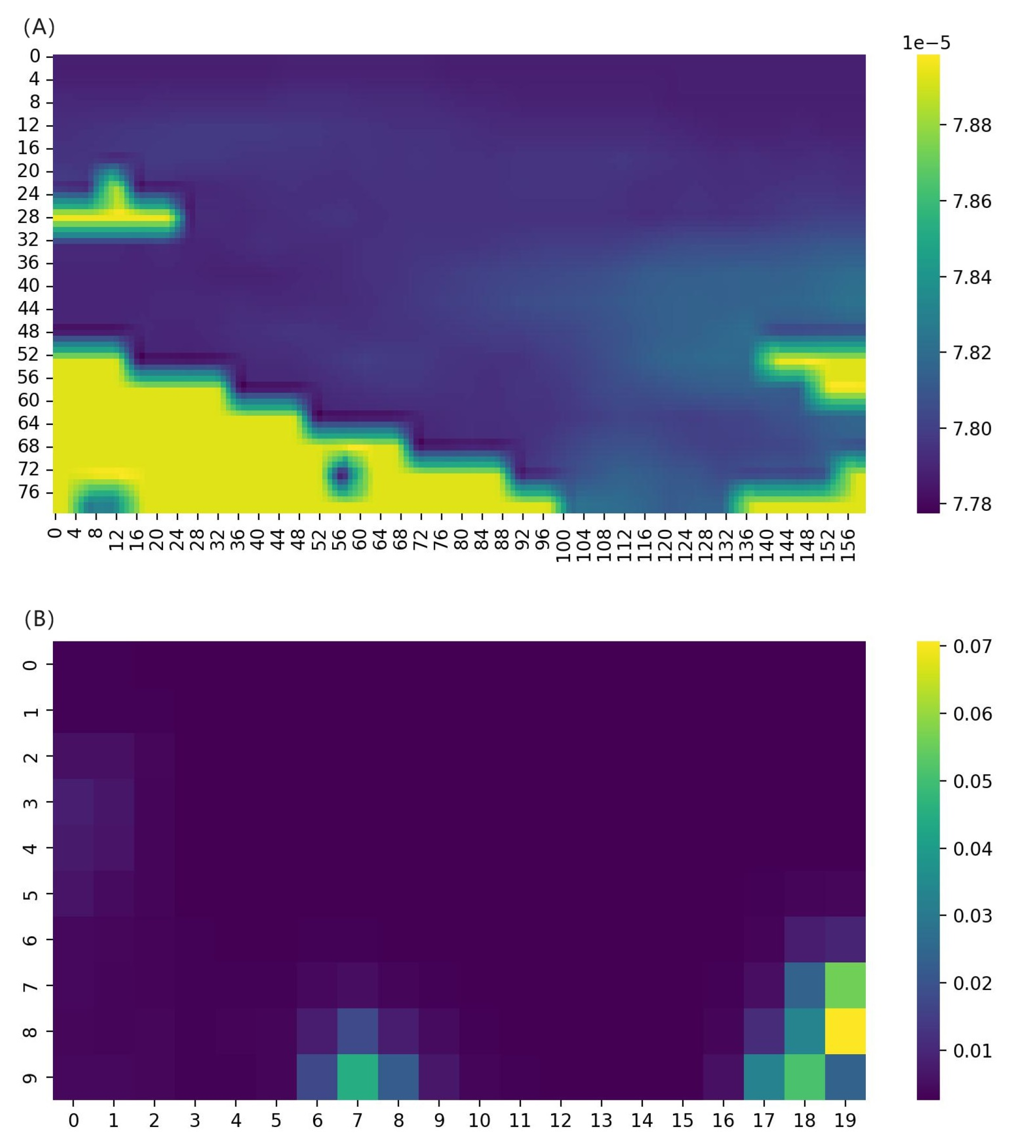
To further explore the spatial behavior of self-attention, we visualized the attention weight distributions at the skip connections of the first and last resolution stages. These results are shown in Figure 11.

Figure 11 presents the weight distribution of the self-attention mechanism in Deep SARU-Net across two resolution stages with skip connections. The color depth corresponds to attention weight magnitude. Figure 11A,B depict the spatial distribution of attention weights for a specific channel. In Figure 11A, representing the highest resolution stage, the weights are concentrated along sea-land boundaries, emphasizing the model’s focus on capturing spatial correlations, which is crucial for distinguishing sea ice from land. Conversely, Figure 11B, at the lowest resolution stage, displays a more dispersed distribution, with heightened attention in key regions, likely corresponding to high SIC areas. This demonstrates that self-attention effectively enhances the model’s ability to capture both local and global sea ice features. These observations confirm that the multi-stage self-attention mechanism enhances the model’s capacity to capture both local and global ice structures.

4.2.7. Model Performance Across Sea Domains and Observation Datasets

Our previous study analyzed Deep SARU-Net’s performance in SIC spatial SR estimation, primarily focusing on the Chukchi Sea. However, this localized evaluation limits our understanding of the model’s generalization across the broader Arctic region. In contrast, mainstream HR SIC numerical models, such as global and polar models, typically achieve spatial resolutions around 1/10°. To assess whether our model can achieve comparable performance, we will conduct experiments evaluating its generalization capability across different Arctic sea regions.

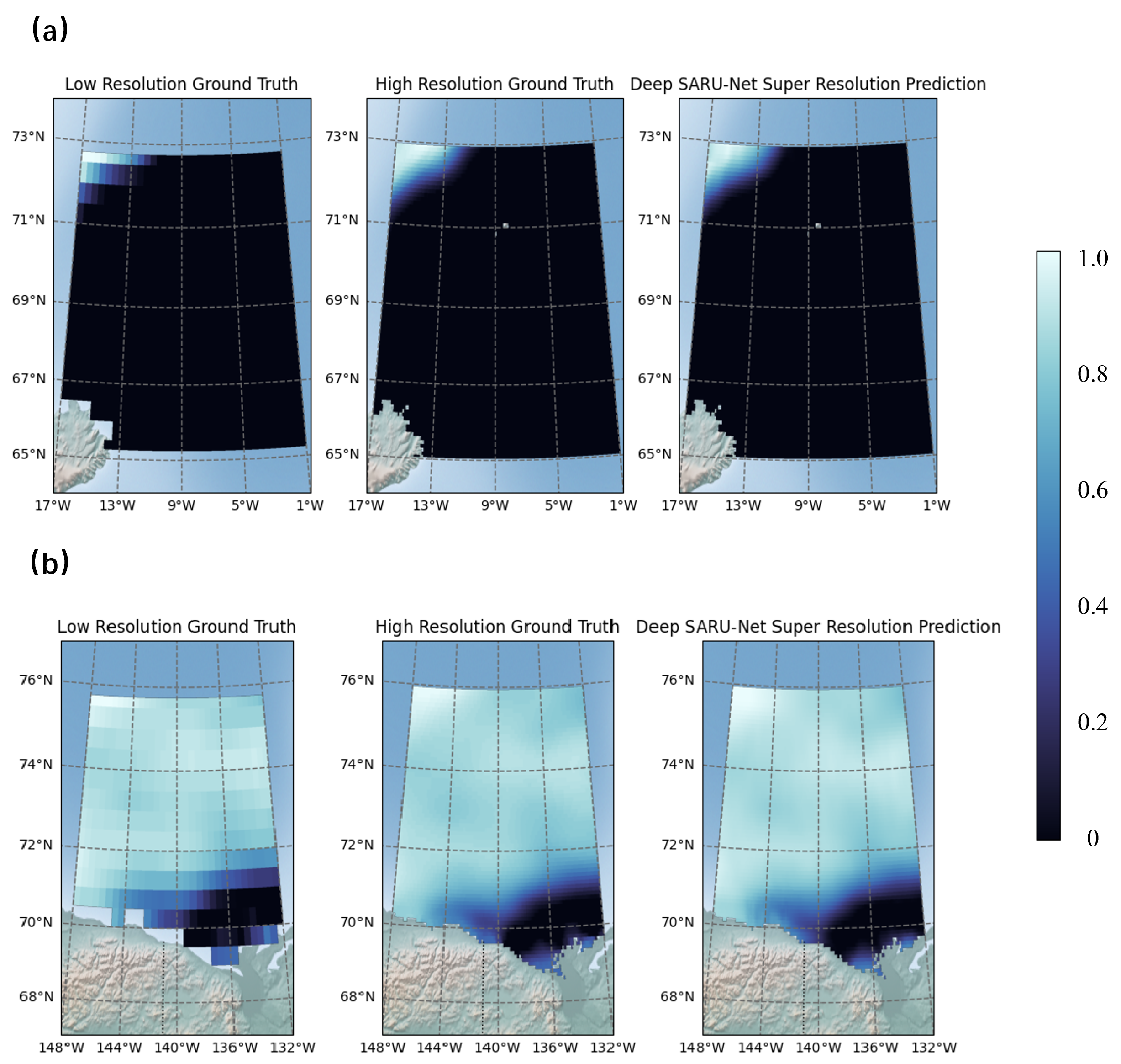
Two additional sea areas, the Beaufort Sea and the Greenland Sea, are chosen for SIC SR estimation studies. The Beaufort Sea, a marginal sea of the Arctic Ocean, remains mostly frozen year-round, with a narrow open-water passage during August to September. Due to Arctic climate change, the ice-free area has expanded, enabling Arctic navigation. The Greenland Sea, part of the Nordic Seas, is important for studies on temperature–salinity circulation and contains potential natural gas and oil resources. These areas were selected to evaluate the model’s generalization performance. OSTIA satellite remote sensing data continue to be selected for the experimental data. The SIC SR results for these regions are shown in Figure 12.

Figure 12 shows the SIC downscaling result by Deep SARU-Net for the two sea regions. In Figure 12a, the model effectively distinguishes sea ice from water, with estimations closely matching HR ground truth and capturing detailed concentration gradients. The model achieves a PSNR of 31.17 dB and an SSIM of 0.9716 in this area. Figure 12b demonstrates the model’s accuracy in capturing the extent and internal concentration of sea ice near Greenland, despite the limited ice coverage, with a PSNR of 40.32 dB and SSIM of 0.9867.

A comprehensive analysis of the SIC SR estimations in these two marine areas shows that our model closely matches HR ground truth, especially in concentration gradients and sea ice distribution continuity. Similar to previous studies in the Chukchi Sea, our model achieves an average RMSE below 0.05 and correlation coefficients above 0.99 across multiple marine areas. This demonstrates that our model’s performance is on par with HR numerical simulations. Additionally, the AI-based Deep SARU-Net model offers significant advantages in terms of parameter efficiency and computational time, while excelling in capturing the detailed distribution and smooth concentration gradients.

In our previous experiments, the SR estimation of SIC was primarily conducted using the OSTIA satellite-derived dataset. Although OSTIA provides relatively high spatial resolution, it is fundamentally generated from passive microwave sensors (e.g., AMSR2, SSMIS) and infrared sensors (e.g., AVHRR) through multi-source data fusion and interpolation. As a result, a substantial portion of the dataset consists of interpolated values rather than direct observations, which reduces its ability to accurately represent fine-scale sea ice structures and ice-edge morphology, particularly under cloudy, harsh-weather, or polar night conditions. In contrast, SAR observations offer significantly higher spatial resolution and, as an active microwave system, can penetrate cloud cover and operate independently of illumination conditions. This enables SAR to capture detailed sea ice texture and ice-edge variations more reliably. However, SAR data also suffer from limited spatial coverage and relatively long revisit intervals, making it difficult to construct large-scale, continuous time-series datasets.

To address these limitations, we adopted a transfer-learning-based strategy: sparse SAR observations were used to retrain and fine-tune the OSTIA-pretrained Deep SARU-Net, enabling us to evaluate its cross-sensor generalization capability and enhance its robustness and applicability for SR estimation under real observational conditions. Specifically, we used 257 days of SAR observations from 2018 to 2021 for fine-tuning. The LR and HR pairs were generated via cubic interpolation of the SAR data. The model was fine-tuned until reconvergence, allowing it to adapt to the spatial patterns and textural characteristics inherent to SAR observations. The fine-tuned model was then applied to the 2022 SAR LR data to estimate SIC, and the results were validated using 64 days of SAR HR data from 2022. The evaluation metrics are summarized in

Table 6. The average RMSE, r, PSNR, and SSIM of SAR observation data for SIC prediction over the 15 days.

Type of Data	RMSE	r	PSNR (dB)	SSIM
SAR	0.0725	0.9744	29.27	0.9361
SAR 56-epochs	0.0535	0.9945	31.22	0.9602
Remote sensing	0.0449	0.9962	32.03	0.9744

.

The results indicate that Deep SARU-Net exhibits strong generalization capability when applied to SAR observations. Using the OSTIA-pretrained weights directly, the model achieved an average RMSE of 0.0725, correlation coefficient r of 0.9744, PSNR of 29.27 dB, and SSIM of 0.9361 on the 2022 validation set, demonstrating that the model can produce reasonably accurate SIC SR estimates even without retraining on SAR data. Furthermore, after fine-tuning with SAR observations, the model required only 56 epochs to reach performance comparable to its OSTIA-based results. The fine-tuned model achieved an RMSE of 0.0535 (a reduction of 26.21%), an r of 0.9945 (an increase of 2.06%), a PSNR of 30.42 dB (an increase of 6.67%), and an SSIM of 0.9602 (an increase of 2.57%). These findings show that Deep SARU-Net can rapidly adapt to SAR-specific characteristics with only limited additional training, achieving SR estimation accuracy similar to that obtained from satellite reanalysis data. This confirms the strong cross-dataset transferability and practical applicability of the proposed model.

4.2.8. Pan-Arctic SR Estimation Performance

Previously, we have validated the capability of Deep SARU-Net for SIC SR estimation in various small Arctic regions. Now, we extend its application to the entire Arctic region to further explore its SR estimation performance on a larger spatial scale. For the study domain, we select the pan-Arctic region (45°N–90°N, −180°W–180°E), which encompasses the Arctic Ocean and its surrounding landmasses, including ecosystems, climate systems, and sociol-economic factors related to the Arctic environment. Conducting SIC SR estimation in this region is crucial for enhancing the precision of Arctic environmental monitoring and estimation.

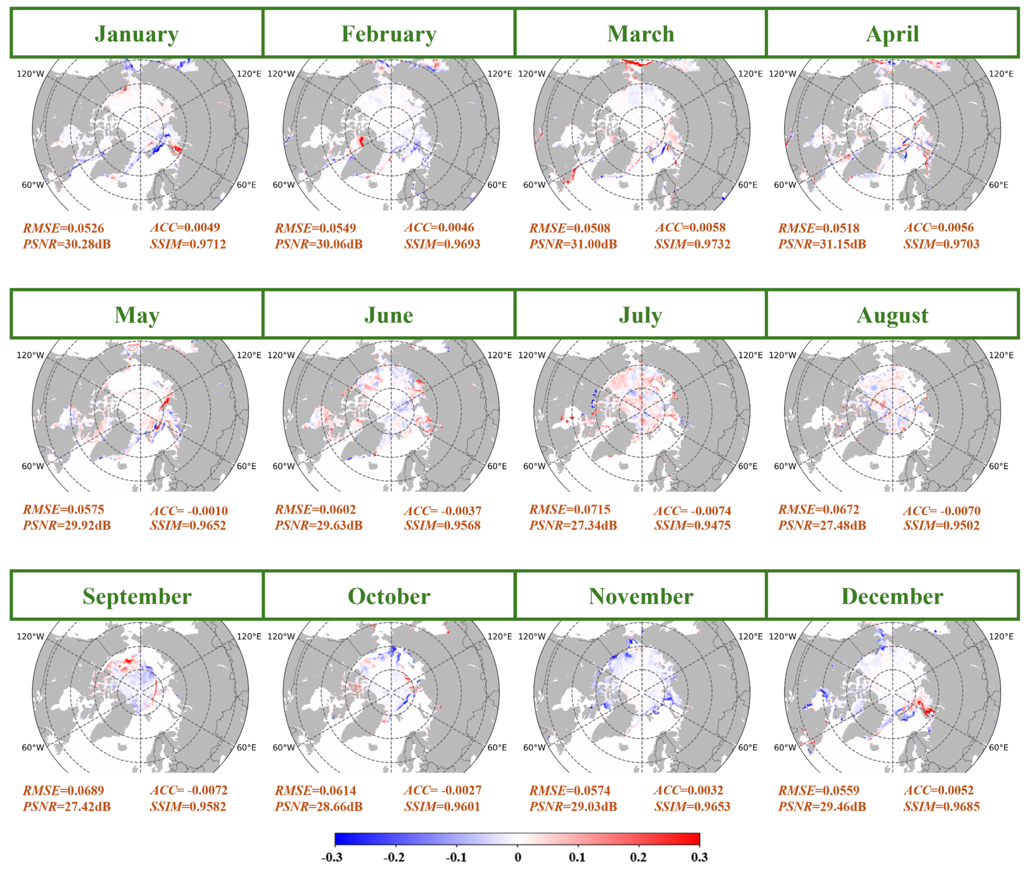
For data selection, we continue to use the OSTIA satellite remote sensing data in our experiments. In earlier stages, a 5× SR factor was adopted to achieve a fine-scale resolution of 1/10° × 1/10° (less than 2 km at high latitudes) to represent detailed SIC structures. However, considering the significant expansion of the study domain, along with constraints on computational cost, hardware resources, and the required level of spatial detail, we have adjusted the SR factor to 2×. Specifically, the LR input data are set to 1/2° × 1/2°, and the HR target data to 1/4° × 1/4°. The Deep SARU-Net is trained under this setting and applied to the pan-Arctic validation set after convergence. Monthly mean estimations are then calculated, and the spatial residuals are visualized in Figure 13.

Although the Pearson correlation coefficient r has been widely used to evaluate overall agreement, it primarily reflects similarity in spatial patterns and is often dominated by the climatological mean. In our experiments, we observed that the monthly average r across the validation set reaches 0.9902, indicating high correlation. However, this high value may mask the model’s ability to capture anomalous sea ice variability, especially during dynamic seasons. To address this limitation, and following the reviewer’s suggestion, we adopt the Anomaly Correlation Coefficient (ACC) as a more meaningful metric. ACC measures the correlation between the reconstructed and observed anomalies—i.e., deviations from the mean state—which better reflects the model’s capacity to reconstruct interannual and spatial fluctuations beyond the climatological baseline. In our analysis, the monthly mean climatology is computed from the training data and subtracted from both the reconstructions and observations before computing ACC.

According to the ACC-based evaluation, Deep SARU-Net demonstrates robust performance across the pan-Arctic region under the 2× SR setting. In winter and spring (January to May), ACC values consistently exceed 0.980, accompanied by RMSE values below 0.0560, PSNR above 30 dB, and SSIM greater than 0.9650—indicating both accurate anomaly reconstruction and high spatial fidelity. During the summer and autumn melting season (June to September), despite greater dynamic complexity, the model still maintains ACC values above 0.960, with RMSE under 0.0750, PSNR above 27 dB, and SSIM above 0.9450. These results confirm that the model effectively captures the evolving deviations from climatology, even under conditions of rapid sea ice retreat.

In terms of spatial residual distribution, the overall residuals of Deep SARU-Net in the 12-month SIC SR estimation range from [−0.3, 0.3], with 95% of the residuals constrained within [−0.2, 0.2]. During January to May and October to December, the residuals in high-latitude regions are nearly zero, with noticeable errors only appearing along the sea ice edges and coastal areas at lower latitudes, primarily within the range of [−0.1, 0.1]. This indicates that the multi-head self-attention mechanism introduced at both the lowest and highest resolution stages effectively enhances the model’s ability to reconstruct variations in SIC, leading to superior performance.

During the melting season from June to September, the rapid retreat of Arctic sea ice significantly increases the difficulty of SR reconstruction. Although the overall sea ice extent decreases, residuals are more widely distributed across the pan-Arctic region. Nevertheless, Deep SARU-Net maintains high estimation accuracy, with errors mostly confined within [−0.15, 0.15] and no significant systematic bias. This suggests that the model effectively constrains the reconstruction of sea ice edges, land-sea transitions, and internal concentration variations, thereby improving the accuracy of spatial distribution reconstruction. These results further confirm that Deep SARU-Net exhibits strong learning capabilities in capturing the spatial distribution patterns of Arctic sea ice, enhancing its SR estimation performance during the melting season, and improving feature representation at sea-land boundaries. These advancements are critical for achieving higher accuracy in SIC SR estimation across the pan-Arctic region.

5. Discussion

In our study, Deep SARU-Net incorporated multi-stage self-attention mechanisms, orthogonal rectangular convolutional kernels, and residual modules. Compared to other SR methods, it significantly improved the predictability of SIC, especially at sea-land boundaries, ice edges, and within regions of SIC variations. This enhancement can be attributed to two main factors. First, data-driven models often introduce prediction biases by relying on correlations without considering physical consistency, leading to deviations from sea ice dynamics. By integrating self-attention, the model can focus on dynamic relationships across time and space, capturing key information related to sea ice processes. Additionally, shallow self-attention mechanisms excel at emphasizing local features, making them effective in reducing biases at coastal boundaries and ice edges.

Despite the significant improvements achieved by Deep SARU-Net, the results reveal a notable seasonal performance disparity: the model performs better in winter (mean RMSE of $0.0337$) compared to summer (RMSE of $0.1274$). This decreased summer predictability can be thoroughly analyzed from both thermodynamic and dynamic perspectives, considering the sea ice heat equation.

$$C_i{\displaystyle \frac{\partial T_i}{\partial t}}=\nabla ·(k_i\nabla T_i)+Q_{net}$$

(7)

where $C_i$ denotes the specific heat capacity of sea ice, $T_i$ is the temperature of sea ice, t is time, $k_i$ represents the heat conductivity coefficient of sea ice and $Q_{net}$ is the net heat flux, taking into account the sum of factors such as solar radiation, atmospheric radiation, and ocean heat exchange.

In summer, increased solar radiation and higher SST lead to greater heat input at both the sea ice surface and the bottom. This accelerates the melting process, altering the temperature gradient within the sea ice system [41]. These changes affect the heat distribution, especially at the sea-land boundaries and sea ice edge, where heat exchange is more frequent [42]. This complexity may contribute to the model’s poorer performance in summer. Furthermore, we then introduce the momentum equation:

$${\rho }_i{\displaystyle \frac{\partial u_i}{\partial t}}=\nabla ·{\sigma }_i+{\rho }_{i}f+F_{\mathrm{ext}}$$

(8)

where ${\rho }_i$ denotes the concentration of sea ice, $u_i$ is the velocity vector of the sea ice, t is time, ${\sigma }_i$ represents the stress tensor, f is the friction within the sea ice and $F_{\mathrm{ext}}$ are external forces exerted on sea ice, such as wind stress and ocean currents.

The Arctic region in summer is prone to strong winds, which generate substantial wind stress and accelerate sea ice movement [43]. Furthermore, higher SST stimulates more vigorous ocean currents, influencing sea ice drift and deformation. These two factors intensify the sea ice velocity and external force terms in the momentum equation, increasing the ice’s speed and deformation and leading to more unstable summer sea ice motion patterns, which further compound the difficulty of summer SIC prediction [44].

To address the summer predictability challenge, we plan to pursue two complementary approaches. On the one hand, from a fully data-driven perspective, future models will incorporate additional proxy features related to sea ice thermodynamic and dynamic processes, including reanalysis-based SST, near-surface air temperature, sea ice velocity, and downward shortwave and longwave radiation. These variables provide critical thermodynamic and dynamic information, potentially alleviating the observed degradation in summer performance. On the other hand, from a physics-constrained perspective, we aim to integrate the sea ice heat and momentum equations (in PDE form) into the SR loss function, introducing thermodynamic and dynamic constraints during neural network optimization to improve summer SIC prediction accuracy.

Beyond the issues mentioned above, our research is also constrained by limitations in the temporal prediction range. Models based on CNNs struggle to capture long-term dependencies in images. Despite the integration of self-attention mechanisms to enhance the model’s focus on temporal scales, significant room for improvement remains in forecasting future multi-day SIC at SR levels. To extend the prediction time range of the model, we plan to incorporate gated units similar to Long Short-Term Memory (LSTM) networks into the current architecture to facilitate the storage and utilization of long-term information. Furthermore, our research will consider integrating Global Navigation Satellite System Reflectometry (GNSS-R) data to enhance sea ice predictive capability [45]. GNSS-R is an emerging remote sensing technique that acquires observational information by receiving echoes from navigation satellite signals (e.g., GPS, Galileo) reflected off the Earth’s surface [46]. Compared to OSTIA data, GNSS-R offers higher spatial resolution. Its L-band signals are highly sensitive to sea ice characteristics and can be used to detect SIC, sea ice thickness, and sea ice extent, particularly in marginal ice zones and regions of newly formed ice, providing unique complementary information. Retraining the model with GNSS-R data could further improve the predictive accuracy and robustness of Deep SARU-Net at fine spatial scales. Finally, we will continue to explore and actively investigate the potential applications of these architectures across diverse prediction tasks.

6. Conclusions

In this study, we propose the Deep SARU-Net architecture to address challenges in reconstructing sea-land boundaries, sea ice edges, and internal concentration variations in sea ice. The architecture incorporates stride convolution with orthogonal rectangular convolution kernels to improve its ability to capture spatial scale information and streamline network parameters. Additionally, residual networks are utilized to preserve as much initial information as possible when spatial scales change, significantly reducing the risk of overfitting. Notably, we also introduce a multi-stage self-attention mechanism to enhance the model’s capacity to capture detailed information and abstract features across different resolution stages.

Firstly, we conduct experiments related to run-time performance and memory requirements. The results demonstrate that the series of structures used in our model effectively decreases the number of trainable parameters without compromising the model’s performance. This method enhances the model’s efficiency and decreases its reliance on computational resources, rendering it more viable. Subsequently, we carry out a sequence of tests to evaluate the model’s performance in the SIC SR estimation task. For comparison, we choose LinearCNN, SRCNN, U-Net, and Attention U-Net as control approaches. Through a thorough analysis of various indicators and estimation results, we determine that the Deep SARU-Net architecture performs well in SIC SR estimation. It is particularly effective in reconstructing the sea-land boundaries, sea ice edges, and internal concentration variations in sea ice. Furthermore, we experimentally identify the parameters of the self-attention mechanism that enable the model to perform optimally, and analyze the reasons for the improved model effectiveness through the results of the self-attention mechanism. In the highest resolution stage, we observed that the attention weights are more focused and primarily highlight the boundaries between the sea and land. This suggests that the network places additional emphasis on the spatial distribution during this stage. At the lowest resolution stage, the model focuses on fewer points of information. These points may represent key information about the input data and may be critical for understanding the overall sea ice distribution. Additionally, we also investigate the generalization of the architecture to different sea areas and prove its universality. The comprehensive experimental results demonstrate that the Deep SARU-Net architecture obtains an RMSE of 0.0449 and a SSIM of 0.9744 for the input sequence length of 5 days, which is a significant improvement relative to other methods. This indicates that the method performs well in reducing the artifact phenomenon and improving the reproduction of image SR reconstruction.

In the Discussion and Outlook sections, we provide a reasonable analysis of the potential factors affecting the model’s performance and discuss possible solutions to the three deficiencies that still exist in the Deep SARU-Net architecture. Particularly, in response to the problem of significant variation in the model’s SR estimation results across different seasons, we begin from the heat and momentum equations of sea ice dynamics. We analyze the reasons for the poor reconstructability effect in summer and propose potential solutions. It is believed that these ideas for solving the problem can provide a favorable reference for future work.

References

1. Jiang, L.; Chen, F.; Yu, D.; Ma, Y.; Zhao, D.; An, D. Automatic High-Accuracy Sea Ice Monitoring in the Arctic Using MODIS Data. IEEE Trans. Geosci. Remote Sens. 2023, 61, 4301413. [Google Scholar] [CrossRef]
2. Meier, W.N.; Hovelsrud, G.K.; van Oort, B.E.; Key, J.R.; Kovacs, K.M.; Michel, C.; Haas, C.; Granskog, M.A.; Gerland, S.; Perovich, D.K.; et al. Arctic sea ice in transformation: A review of recent observed changes and impacts on biology and human activity. Rev. Geophys. 2014, 52, 185–217. [Google Scholar] [CrossRef]
3. Yercan, F.; Ziya Sogut, M. Comparative analysis of entropy and environmental impacts of shipping operations on arctic and international routes. Appl. Ocean Res. 2023, 139, 103707. [Google Scholar] [CrossRef]
4. Liu, J.; Chen, L.; Liu, Y. A statistical downscaling prediction model for winter temperature over Xinjiang based on the CFSv2 and sea ice forcing. Int. J. Climatol. 2022, 42, 8552–8567. [Google Scholar] [CrossRef]
5. Wulf, T.; Buus-Hinkler, J.; Singha, S.; Shi, H.; Kreiner, M.B. Pan-Arctic sea ice concentration from SAR and passive microwave. Cryosphere 2024, 18, 5277–5300. [Google Scholar] [CrossRef]
6. Adler, J.; Kawulok, J.; Kawulok, M. Toward Understanding the Impact of Input Data for Multi-Image Super-Resolution. In Proceedings of the Intelligent Information and Database Systems, Ho Chi Minh City, Vietnam, 28–30 November 2022; Nguyen, N.T., Tran, T.K., Tukayev, U., Hong, T.P., Trawiński, B., Szczerbicki, E., Eds.; Springer Nature: Cham, Switzerland, 2022; pp. 329–342. [Google Scholar] [CrossRef]
7. Feng, T.; Liu, X.; Li, R. Super-Resolution-Aided Sea Ice Concentration Estimation From AMSR2 Images by Encoder–Decoder Networks With Atrous Convolution. IEEE J. Sel. Top. Appl. Earth Obs. Remote Sens. 2023, 16, 962–973. [Google Scholar] [CrossRef]
8. Wilby, R.; Wigley, T. Downscaling general circulation model output: A review of methods and limitations. Prog. Phys. Geogr. 1997, 21, 530–548. [Google Scholar] [CrossRef]
9. Wilby, R.; Wigley, T. Precipitation predictors for downscaling: Observed and general circulation model relationships. Int. J. Climatol. 2000, 20, 641–661. [Google Scholar] [CrossRef]
10. Shukla, R.; Khare, D.; Kumar Dwivedi, A.; Rudra, R.P.; Palmate, S.S.; Ojha, C.S.P.; Singh, V.P. Evaluation of statistical downscaling model’s performance in projecting future climate change scenarios. J. Water Clim. Chang. 2023, 14, 3559–3595. [Google Scholar] [CrossRef]
11. He, J.; Zhao, Y.; Yang, D.; Wang, H.; Deng, X. Physically Constrained Spatiotemporal Deep Learning Model for Fine-Scale, Long-Term Arctic Sea Ice Concentration Prediction. IEEE Trans. Geosci. Remote Sens. 2025, 63, 4300921. [Google Scholar] [CrossRef]
12. Yuan, S.; Zhu, S.; Luo, X.; Mu, B. A deep learning-based bias correction model for Arctic sea ice concentration towards MITgcm. Ocean Model. 2024, 188, 102326. [Google Scholar] [CrossRef]
13. Zhao, Y.; Yang, D.; He, J.; Zhu, K.; Deng, X. Hierarchical stacked spatiotemporal self-attention network for sea surface temperature forecasting. Ocean Model. 2024, 191, 102427. [Google Scholar] [CrossRef]
14. Rocha, M.; Lynch, A.; Bergen, K. Enhancing sea ice concentration resolution in a northern sea route strait using a generative adversarial network. J. Geophys. Res. Mach. Learn. Comput. 2025, 2, e2024JH000281. [Google Scholar] [CrossRef]
15. Karamouz, M.; Nazif, S.; Fallahi, M. Rainfall Downscaling Using Statistical Downscaling Model and Canonical Correlation Analysis: A Case Study. In Proceedings of the World Environmental and Water Resources Congress, Providence, RI, USA, 16–20 May 2010; pp. 4579–4587. [Google Scholar] [CrossRef]
16. Liu, Y.; Fan, K. A new statistical downscaling model for autumn precipitation in China. Int. J. Climatol. 2013, 33, 1321–1336. [Google Scholar] [CrossRef]
17. Liu, X.; Feng, T.; Shen, X.; Li, R. PMDRnet: A Progressive Multiscale Deformable Residual Network for Multi-Image Super-Resolution of AMSR2 Arctic Sea Ice Images. IEEE Trans. Geosci. Remote Sens. 2022, 60, 4304118. [Google Scholar] [CrossRef]
18. Feng, T.; Jiang, P.; Liu, X.; Ma, X. Applications of Deep Learning-Based Super-Resolution Networks for AMSR2 Arctic Sea Ice Images. Remote Sens. 2023, 15, 5401. [Google Scholar] [CrossRef]
19. Men, P.; Guo, H.; An, J.; Li, G. Large-Resolution Difference Heterogeneous SAR Image Sea Ice Drift Tracking Using a Smooth Edge-Guide Super-Resolution Residual Network. IEEE Trans. Geosci. Remote Sens. 2023, 61, 5212519. [Google Scholar] [CrossRef]
20. Li, W.; Hsu, C.Y.; Tedesco, M. Advancing Arctic sea ice remote sensing with AI and deep learning: Now and future. Remote Sens. 2024, 16, 3764. [Google Scholar] [CrossRef]
21. Chen, S.; Li, K.; Fu, H.; Wu, Y.C.; Huang, Y. Sea Ice Extent Prediction with Machine Learning Methods and Subregional Analysis in the Arctic. Atmosphere 2023, 14, 1023. [Google Scholar] [CrossRef]
22. Ronneberger, O.; Fischer, P.; Brox, T. U-Net: Convolutional Networks for Biomedical Image Segmentation. In Proceedings of the Medical Image Computing and Computer-Assisted Intervention—MICCAI 2015, Munich, Germany, 5–9 October 2015; Navab, N., Hornegger, J., Wells, W.M., Frangi, A.F., Eds.; Springer Nature: Cham, Switzerland, 2015; pp. 234–241. [Google Scholar] [CrossRef]
23. He, K.; Zhang, X.; Ren, S.; Sun, J. Deep residual learning for image recognition. In Proceedings of the IEEE Conference on Computer Vision and Pattern Recognition, Las Vegas, NV, USA, 27–30 June 2016; pp. 770–778. [Google Scholar] [CrossRef]
24. Vaswani, A.; Shazeer, N.; Parmar, N.; Uszkoreit, J.; Jones, L.; Gomez, A.N.; Kaiser, L.u.; Polosukhin, I. Attention is All you Need. In Proceedings of the Advances in Neural Information Processing Systems, Long Beach, CA, USA, 4–9 December 2017; Guyon, I., Luxburg, U.V., Bengio, S., Wallach, H., Fergus, R., Vishwanathan, S., Garnett, R., Eds.; Curran Associates, Inc.: New York, NY, USA, 2017; Volume 30. [Google Scholar]
25. Höhlein, K.; Kern, M.; Hewson, T.; Westermann, R. A comparative study of convolutional neural network models for wind field downscaling. Meteorol. Appl. 2020, 27, e1961. [Google Scholar] [CrossRef]
26. Wang, Z.; Bovik, A.; Sheikh, H.; Simoncelli, E. Image quality assessment: From error visibility to structural similarity. IEEE Trans. Image Process. 2004, 13, 600–612. [Google Scholar] [CrossRef]
27. Liu, Z.; Yan, W.Q.; Yang, M.L. Image denoising based on a CNN model. In Proceedings of the 2018 4th International Conference on Control, Automation and Robotics (ICCAR), Auckland, New Zealand, 20–23 April 2018; pp. 389–393. [Google Scholar] [CrossRef]
28. Dong, C.; Loy, C.C.; He, K.; Tang, X. Image Super-Resolution Using Deep Convolutional Networks. IEEE Trans. Pattern Anal. Mach. Intell. 2016, 38, 295–307. [Google Scholar] [CrossRef]
29. Siddique, N.; Paheding, S.; Elkin, C.P.; Devabhaktuni, V. U-Net and Its Variants for Medical Image Segmentation: A Review of Theory and Applications. IEEE Access 2021, 9, 82031–82057. [Google Scholar] [CrossRef]
30. Oktay, O.; Schlemper, J.; Folgoc, L.L.; Lee, M.; Heinrich, M.; Misawa, K.; Mori, K.; McDonagh, S.; Hammerla, N.Y.; Kainz, B.; et al. Attention U-Net: Learning Where to Look for the Pancreas. arXiv 2018, arXiv:1804.03999. [Google Scholar] [CrossRef]
31. Temenos, A.; Temenos, N.; Doulamis, A.; Doulamis, N. On the Exploration of Automatic Building Extraction from RGB Satellite Images Using Deep Learning Architectures Based on U-Net. Technologies 2022, 10, 19. [Google Scholar] [CrossRef]
32. Paszke, A.; Gross, S.; Massa, F.; Lerer, A.; Bradbury, J.; Chanan, G.; Killeen, T.; Lin, Z.; Gimelshein, N.; Antiga, L.; et al. Pytorch: An imperative style, high-performance deep learning library. Adv. Neural Inf. Process. Syst. 2019, 32. [Google Scholar]
33. He, K.; Zhang, X.; Ren, S.; Sun, J. Delving Deep into Rectifiers: Surpassing Human-Level Performance on ImageNet Classification. In Proceedings of the IEEE International Conference on Computer Vision (ICCV), Santiago, Chile, 7–13 December 2015. [Google Scholar] [CrossRef]
34. Ioffe, S.; Szegedy, C. Batch normalization: Accelerating deep network training by reducing internal covariate shift. In Proceedings of the International Conference on Machine Learning, PMLR, Lille, France, 6–11 July 2015; pp. 448–456. [Google Scholar]
35. Kingma, D.P.; Welling, M. Auto-encoding variational bayes. arXiv 2013, arXiv:1312.6114. [Google Scholar] [CrossRef]
36. Srivastava, N.; Hinton, G.; Krizhevsky, A.; Sutskever, I.; Salakhutdinov, R. Dropout: A simple way to prevent neural networks from overfitting. J. Mach. Learn. Res. 2014, 15, 1929–1958. [Google Scholar]
37. Donlon, C.J.; Martin, M.; Stark, J.; Roberts-Jones, J.; Fiedler, E.; Wimmer, W. The Operational Sea Surface Temperature and Sea Ice Analysis (OSTIA) system. Remote Sens. Environ. 2012, 116, 140–158. [Google Scholar] [CrossRef]
38. Good, S.; Fiedler, E.; Mao, C.; Martin, M.J.; Maycock, A.; Reid, R.; Roberts-Jones, J.; Searle, T.; Waters, J.; While, J.; et al. The Current Configuration of the OSTIA System for Operational Production of Foundation Sea Surface Temperature and Ice Concentration Analyses. Remote Sens. 2020, 12, 720. [Google Scholar] [CrossRef]
39. Stark, J.D.; Donlon, C.J.; Martin, M.J.; McCulloch, M.E. OSTIA: An operational, high resolution, real time, global sea surface temperature analysis system. In Proceedings of the Oceans 2007-Europe, Aberdeen, UK, 18–21 June 2007; pp. 1–4. [Google Scholar] [CrossRef]
40. Huang, Y.; Niu, B.; Guan, H.; Zhang, S. Enhancing image watermarking with adaptive embedding parameter and PSNR guarantee. IEEE Trans. Multimed. 2019, 21, 2447–2460. [Google Scholar] [CrossRef]
41. Dai, G.; Mu, M.; Han, Z.; Li, C.; Jiang, Z.; Zhu, M.; Ma, X. The Influence of Arctic Sea Ice Concentration Perturbations on Subseasonal Predictions of North Atlantic Oscillation Events. Adv. Atmos. Sci. 2023, 40, 2242–2261. [Google Scholar] [CrossRef]
42. Polyakov, I.V.; Mayer, M.; Tietsche, S.; Karpechko, A.Y. Climate change fosters competing effects of dynamics and thermodynamics in seasonal predictability of Arctic sea ice. J. Clim. 2022, 35, 2849–2865. [Google Scholar] [CrossRef]
43. Lukovich, J.V.; Stroeve, J.C.; Crawford, A.; Hamilton, L.; Tsamados, M.; Heorton, H.; Massonnet, F. Summer Extreme Cyclone Impacts on Arctic Sea Ice. J. Clim. 2021, 34, 4817–4834. [Google Scholar] [CrossRef]
44. Yi, D.L.; Fan, K.; He, S. Thermodynamic and dynamic contributions to the abrupt increased winter Arctic sea ice growth since 2008. Environ. Res. Lett. 2023, 19, 014048. [Google Scholar] [CrossRef]
45. Munoz-Martin, J.F.; Rodriguez-Alvarez, N.; Bosch-Lluis, X.; Oudrhiri, K. Integrated retrieval of sea-ice salinity, density, and thickness using polarimetric GNSS-R. Remote Sens. Environ. 2025, 318, 114617. [Google Scholar] [CrossRef]
46. Hu, Y.; Hua, X.; Yan, Q.; Liu, W.; Jiang, Z.; Wickert, J. Sea ice detection from GNSS-R data based on local linear embedding. Remote Sens. 2024, 16, 2621. [Google Scholar] [CrossRef]
Figure 1. The convolution operation result after replacing the square 3 × 3 kernel with two rectangular kernels, one of size 3 × 1 and the other of size 1 × 3.
Remotesensing 17 03839 g001
Figure 2. Illustration of multi-head attention mechanisms. Each attention head in the multi-head attention mechanism is an independent attention mechanism. The multi-head attention mechanism allows us to simultaneously focus on different positions in the input sequence.
Remotesensing 17 03839 g002
Figure 3. Network Architecture of Deep SARU-Net.
Remotesensing 17 03839 g003
Figure 4. The primary study domain of this research is the Chukchi Sea, as indicated by Region 1 in the figure. The Beaufort Sea and the Greenland Sea, labeled as Regions 2 and 3, respectively, are used to evaluate the model’s generalization capability.
Remotesensing 17 03839 g004
Figure 5. Boxplots depict the distribution of RMSE on the validation set for various models with input durations of 1 day (top left), 3 days (top right), 5 days (bottom left), and 7 days (bottom right). In the experiments, when the input duration is set to 7 days, the four deep models, U-Net, Attention U-Net, PMDRnet, and Deep SARU-Net, exhibit over-fitting on the validation set.
Remotesensing 17 03839 g005
Figure 6. Performance evaluation results of SIC SR estimation under different attention head numbers. The left vertical axis in the figure represents he total training procedure duration, while the right vertical axis represents the RMSE of the model.
Remotesensing 17 03839 g006
Figure 7. Training and validation loss curves for the Deep SARU-Net. he curve indicates that SSIM stabilizes around 300 epochs, and no noticeable over-fitting is observed across the entire validation dataset.
Remotesensing 17 03839 g007
Figure 8. The spatial distribution maps of SIC SR estimation results are presented in this figure. The left panel corresponds to the first half of 2022 (1 June 2022), while the right panel depicts the second half of 2022 (28 December 2022). The first row displays the SIC LR ground truth, HR ground truth, and the SR estimation results obtained with Deep SARU-Net. The second row, from left to right, presents the results of bilinear interpolation, LinearCNN, and SRCNN. The third row, from left to right, shows the SR estimation results produced by U-Net, Attention U-Net, and PMDRnet.
Remotesensing 17 03839 g008
Figure 9. The spatial distribution maps of residuals for SIC SR estimations. (A) presents the residual outcomes for the first half of 2022 (1 June 2022), while (B) depicts those for the second half of 2022 (28 December 2022). The first row displays the residual distribution produced by Deep SARU-Net. The second row, from left to right, shows the residuals obtained from bilinear interpolation, LinearCNN, and SRCNN. The third row, also from left to right, illustrates the residual distributions generated by U-Net, Attention U-Net, and PMDRnet.
Remotesensing 17 03839 g009
Figure 10. The kernel density estimates (KDE) curves for residual estimations in SIC SR across seven models.
Remotesensing 17 03839 g010
Figure 11. Heat maps of the self-attention mechanism weights. (A) illustrates the situation in the first resolution stage, taking one channel as an example, with a grid size of 80 × 160. (B) depicts the situation in the last resolution stage, also using one channel as an example, with a grid size of 10 × 20.
Remotesensing 17 03839 g011
Figure 12. SIC SR estimation results for the two sea domains. From left to right, the figures represent the LR ground truth, HR ground truth, and the SR estimation result for SIC. (a) corresponds to the region near the Beaufort Sea, while (b) corresponds to the region near the Greenland Sea.
Remotesensing 17 03839 g012
Figure 13. The month average SIC downscaling estimation delta on the validation set. The figure also presents the monthly average RMSE, Anomaly Correlation Coefficient (ACC), PSNR, and SSIM.
Remotesensing 17 03839 g013