Speckle2Self: Learning Self-Supervised Despeckling with Attention Mechanism for SAR Images

Highlights

What are the main findings?

• A novel self-supervised despeckling framework, Speckle2Self, is proposed for SAR images, which learns directly from noisy inputs without requiring clean reference data or temporal image sequences.
• The method models despeckling as a masked pixel estimation problem using a Transformer backbone and attention-guided complementary masks, enabling effective noise suppression while preserving structural details.

What is the implication of the main finding?

• The proposed Speckle2Self achieves despeckling performance comparable to supervised approaches, significantly advancing the feasibility of reference-free SAR image restoration.
• This framework provides a robust and generalizable solution for SAR despeckling, facilitating improved image quality and enhanced performance in downstream remote sensing applications.

Abstract

Despite the in-depth understanding of the synthetic aperture-radar (SAR) speckle and its characteristics, despeckling remains an open issue far from being solved. Deep-learning methods with supervised training have made great progress. However, reliable reference images are inconveniently accessible or even non-existent. In this paper, we propose an end-to-end self-supervised method named Speckle2Self for SAR image despeckling, which learns mapping from noisy input to clean output using only the input noisy image itself for training. We formulate the image despeckling as a masked pixel-estimation problem, where a set of masks is carefully designed. The masked pixel values are predicted by the queries of complementary masks indicating the positions of masked pixels through an attention mechanism. Transformer architecture is employed as the network backbone. In addition, a novel loss function is also derived based on the statistics of SAR images, and meanwhile, image downsampling is used to provide guarantees on the white noise assumption involved in our Speckle2Self. We compare the proposed Speckle2Self with reference methods on both synthetic and real images. Experimental results demonstrate that the proposed Speckle2Self achieves comparable despeckling performance with supervised methods, suppressing noise while maintaining structural details. Even compared with self-supervised methods, the proposed Speckle2Self still has significant advantages in SAR image-despeckling metrics.

1. Introduction

Synthetic aperture radar (SAR) is an important microwave remote-sensing technique, offering complementary information to common optical imaging. Speckle is a physical phenomenon caused by the coherent sum of contributions from different elementary scatterers within the same resolution cell [1,2]. The presence of speckle affects performances in various applications of SAR image processing. For example, it increases the false-alarm rate in target detection [3] and decreases the classification accuracy in terrain classification [4]. To improve the quality of SAR images and promote downstream task performances, speckle has to be reduced.

During the past three decades, many despeckling methods have been proposed. Distinguished from the processing domain, SAR despeckling methods can be broadly categorized into spatial-domain methods and transform-domain methods.

Spatial-domain methods [5,6,7] directly process image pixels and usually operate in a sliding-window fashion. The intensive smoothing of nearly simple average causes the loss of structure information. The minimum mean square error (MMSE) criterion [8,9,10] or the maximum a posteriori (MAP) criterion [11,12,13] are used to perform spatial filtering. These methods improve the preservation of features in speckle filtering, however, artifacts are also introduced along feature boundaries. To overcome this problem, Lee et al. [14] proposed neighboring pixel selection based on scattering characteristics.

Transform-domain methods work with additive noise via homomorphic transformation [15] by taking the logarithm of the noisy image. The denoising methods developed for the additive noise case can be applied to the logarithmic SAR image, such as total variation [16], wavelet shrinkage [17,18], and sparse representation [19,20]. Xu et al. [21] proposed a coarse-to-fine filtering approach via patch ordering in THE transform domain, which was followed by an iterative version [22].

Another research line is about non-local approaches. The basic idea is to take advantage of the self-similarity commonly present in natural as well as SAR images. The pioneering work is represented by the non-local mean (NLM) filter [23]. The NLM algorithm has also been extended to SAR [24,25,26,27] image despeckling. Inspired by the block matching 3-D (BM3D) algorithm [28], Parrilli et al. [29] proposed a SAR version of BM3D, i.e., SAR-BM3D, using local linear-MMSE criterion and undecimated wavelet. SAR-BM3D has exhibited promising performance in despeckling studies.

The great success of deep neural networks (NNs) on many tasks involving image processing has shown its powerful learning capabilities and the remote sensing community is starting to exploit the potential of NNs for SAR image despeckling. The SAR-convolutional neural network (SAR-CNN) [30] was the first attempt to denoise SAR image by applying residual-based CNN. Several subsequent deep-learning works [31,32,33,34] proposed slight variations on the topic by introducing different network architectures and loss functions in supervised framework. In [31], a dilated residual network using skip connections was used to train a deep neural network for SAR image despeckling. More recently, Pan et al. [33] dealt with the unknown noise statistics in SAR images by embedding a CNN model for additive white Gaussian noise reduction with a multi-channel logarithm with Gaussian denoising (MuLoG), first introduced in [35]. Furthermore, Vitale et al. [34] proposed a multi-objective network (MONet) by considering loss function as a balanced combination of the spatial details, speckle statistics, and strong scatterer identification of SAR images.

Since noise-free reference images are not available, it is an important issue to construct simulated data and corresponding references. Wang et al. [36] used natural images to produce SAR-like data. The natural image dataset BSD500 [37] was used in [38,39,40], while Google Maps [41] and the University of California, Merced [42] were employed in [43,44,45,46,47,48], respectively. The data generation offers the possibility to train big models but also implicitly implants fatal flaws into trained models. For example, it requires assuming an a priori speckle-noise model, which may not match real SAR data. In addition, the artificial combination of synthetic noise and natural images does not represent the true appearance of SAR images in plenty of aspects, such as edge and texture scattering. Thus, Cozzolino et al. [49,50], Tan et al. [51], and Tang et al. [52] created reference images by exploiting a temporal series of images: assuming that no change had occurred between acquisitions, the temporal average could be used as a proxy for the reference label. This approach, though appealing, has two obvious limits. First, 25 or even 50 images are not enough to adequately approximate a clean infinite-look reference [53,54]. Second, when the scene under investigation is non-stationary over time, taking the temporal average will result in erroneous estimation of the reference label, greatly limiting the applicability of such approaches.

As discussed, supervised methods suffer the lack of noisy-free references. For this reason, the past year has witnessed growing interest in self-supervised methods [55,56,57,58,59,60,61,62,63,64,65,66,67,68,69]. For instance, an adversarial learning framework was employed in [60] to generate images of the same scene with different speckle realizations. A different solution was presented in [67,68], where the network was trained for initialization using a temporally averaged SAR image as a reference label. After preliminary training, the network was fine-tuned without using any clean reference labels. In addition, the works in [66,69] extended the single-image blind-spot approach of [57,59] and proposed a self-supervised Bayesian framework for SAR despeckling.

Upon reviewing the literature, it is evident that filtering methods for optical images cannot be directly applied to SAR images due to their unique speckle characteristics. Current SAR image filtering methods that rely on supervised training are contingent upon the availability of pristine image references, which are often difficult to acquire or may not exist at all. Existing self-supervised SAR filtering methods have several limitations: they fail to achieve end-to-end training and inference, do not fully consider the specific noise distribution of SAR images, and do not address the issue of white-noise assumptions in self-supervision.

To address existing challenges, we propose Speckle2Self: a self-supervised NN method for SAR image despeckling, which uses input noisy images only for training. Neither synthetic data nor temporal series data are required, avoiding the domain gap caused by the mismatching between training data and real test data. The proposed Speckle2Self is an end-to-end method that does not require pre-processing or post-processing. The speckle characteristics are fully considered and noise-whitening problem is solved through image downsampling. Specifically, we design mask sets for image blinding and employ a Transformer encoder to achieve contextual information pooling of masked images. Complementary masks are innovatively used as queries for masked pixel prediction. Our main contributions can be summarized as follows:

• We propose an end-to-end self-supervised despeckling approach named Speckle2Self for SAR images with Transformer architecture. The proposed Speckle2Self models the image despeckling as a masked-pixel estimation problem, where a set of masks is carefully designed. The final despeckled results are given by the Transformer queries indicating the positions of masked pixels, under the guidance of attention mechanism.
• We introduce a novel loss function that fully considers the statistical properties of SAR images, outperforming traditional $l_1$ and $l_2$ loss functions. Noise whitening is achieved through image downsampling, ensuring the validity of the white-noise assumption in our self-supervised method.
• The proposed Speckle2Self method achieves despeckling performance comparable to supervised methods, effectively suppressing noise while preserving structural details. Compared with the other self-supervised method, Speckle2Self also demonstrates significant advantages.

Among all the literature, the one similar to this article is Speckle2Void, the work in [69]. It is worth mentioning the main differences between them:

• They have different problem formulations. Speckle2Void employs NNs to estimate the parameters of the prior distribution of the noise, and generates despeckled results by combining the estimated parameters and a constructed MMSE estimator. On the contrary, in our method, the network operates directly on image data, taking the noisy image as input and outputting a denoised version.
• They use different loss functions and implementations of blind-spot network structures. The loss function of Speckle2Void is derived in the spatial domain, while ours is derived in the transform domain. And the blind-spot network is implemented by four convolutional neural network branches in Speckle2Void, while we choose a simpler way and implement such a structure through a series of carefully designed masks.
• They have different network architectures. The network mainbody of Speckle2Void is a CNN-based U-net [70], while we use Transformer architecture as the backbone.
• Speckle2Void relies on noise level priors and requires the noise level as an input parameter, while our proposed Speckle2Void is a blind filter, and has wider applications.

The rest of the paper is organized as follows: Section 2 introduces the related work. Section 3 presents the proposed method in detail, including the loss function, network architecture, training and despeckling schemes. Section 4 reports the experimental results and discussions. Finally, Section 5 concludes this paper.

2. Background

2.1. Self-Supervised Denoising with NNs

The authors of Noise2Noise [55] find that it is possible to learn to restore images by only looking at corrupted examples without explicit image priors. Image denoising with NNs can be described as an empirical risk minimization problem:

$$\underset{\theta }{argmin}\sum _i\mathcal{L}\left(f_{\theta }\left({\mathit{y}}_i\right),{\mathit{x}}_i\right),$$

(1)

where $f_{\theta }$ is a parametric family of mapping (e.g., NNs) under the loss function $\mathcal{L}$ and ${\mathit{y}}_i$ and ${\mathit{x}}_i$ are the corrupted input and clean reference of the ith sample pair $({\mathit{y}}_i,{\mathit{x}}_i)$, respectively. With some simple assumptions, the estimate remains unchanged if we replace the target with random variables whose expectations match the target references. This implies that we can corrupt the training references of a neural network with zero-mean noise without changing what the network learns [55]. The minimization problem (1) can be re-expressed as

$$\underset{\theta }{argmin}\sum _i\mathcal{L}\left(f_{\theta }\left({\mathit{y}}_i\right),{\mathit{x}}_i+{\mathit{n}}_i\right),$$

(2)

where ${\mathit{n}}_i$ is zero-mean noise and $\mathbb{E}\left({\mathit{n}}_i\right)=0$. In other words, Noise2Noise [55] attempts to train a network with a large number of pairs $({\mathit{y}}_i,{{\mathit{y}}_i}^{\prime })$, where ${\mathit{y}}_i$ and ${{\mathit{y}}_i}^{\prime }$ are pairs of independently degraded versions of the same training image. Noise2Noise training requires pairs of noisy images of the same clean image, with independent zero-mean noise.

Noise2Void [56] takes the idea of Noise2Noise one step further. It does not use noisy pairs, nor clean reference images, but just noisy images only. Two simple statistical assumptions are made in Noise2Void: (1) the pixel value ${\mathit{x}}_i$ is not pixel-wise independent, (2) the noise ${\mathit{n}}_i$ is conditionally pixel-wise independent given x. Denote the jth pixel of the target reference image ${\mathit{x}}_i$ as $x_i^j$. Equation (1) can be rewritten as

$$\underset{\theta }{argmin}\sum _i\sum _j\mathcal{L}\left(f_{\theta }{\left({\mathit{y}}_i\right)}^j,x_i^j\right),$$

(3)

where $f_{\theta }{\left({\mathit{y}}_i\right)}^j$ is the jth pixel of the network output $f_{\theta }\left({\mathit{y}}_i\right)$. In general, each pixel in the output of the CNN has a certain receptive field upon its input. Following this view,

$$\underset{\theta }{argmin}\sum _i\sum _j\mathcal{L}\left(f_{\theta }\left(y_i^{R{F}_j}\right),x_i^j\right),$$

(4)

where $y_i^{R{F}_j}$ is a patch around pixel j, that is, the receptive field. With the conclusion of Noise2Noise, the clean target $x_i^j$ can be replaced by noisy target $y_i^j\prime =x_i^j+n_i^j\prime$. To make full use of noisy training sample, the authors propose to use $y_i^j$ directly as the noisy target. And the pixel j is masked in the receptive field $y_i^{R{F}_j}$ to prevent the network from learning identity. The network trained in this masked way is called the blind-spot network. Consequently, the CNN is defined as

$$f_{\theta }\left(y_i^{R{F}_j\setminus j}\right)={\widehat{x}}_i^j,$$

(5)

where $y_i^{R{F}_j\setminus j}$ is $y_i^{R{F}_j}$, excluding $y_i^j$. And the CNN is trained by minimizing pixel-wise loss:

$$\underset{\theta }{argmin}\sum _i\sum _j\mathcal{L}\left(f_{\theta }\left(y_i^{R{F}_j\setminus j}\right),y_i^j\right).$$

(6)

2.2. Vanilla Transformer with Attention Mechanism

As a sequence-to-sequence model, the vanilla Transformer [71] consists of an encoder and a decoder, each of which is a stack of identical blocks. Each encoder block is mainly composed of a multi-head self-attention module and a position-wise feed-forward network (FFN) [41]. And residual connections [72] and layer normalizations [73] are also employed. Compared with the encoder blocks, decoder blocks adapt self-attention modules to masked self-attention modules and cross-attention modules by masking and replacing the corresponding inputs. In the following, we shall introduce the key modules of the vanilla Transformer.

2.2.1. Attention Modules

The Transformer adopts scaled dot-product attention, which can be described as mapping queries and a set of key–value pairs to outputs. Given the packed matrix representations of queries $\mathbf{Q}\in {\mathbb{R}}^{N\times d_k}$, keys $\mathbf{K}\in {\mathbb{R}}^{M\times d_k}$, and values $\mathbf{V}\in {\mathbb{R}}^{M\times d_v}$, the attention used is given by

$$\mathrm{Attention}(\mathbf{Q},\mathbf{K},\mathbf{V})=\mathrm{softmax}\left({\displaystyle \frac{\mathbf{Q}{\mathbf{K}}^T}{\sqrt{d_k}}}\right)\mathbf{V},$$

(7)

where N and M denote the lengths of queries and keys (or values), $d_k$ and $d_v$ denote the dimensions of keys (or queries) and values. The dot-products of queries and keys are divided by $\sqrt{d_k}$ to the alleviate gradient vanishing problem of the softmax function.

The Transformer uses the attention module in three different ways [71]:

• Self-attention. In Transformer encoder, we set $\mathbf{Q}=\mathbf{K}=\mathbf{V}=\mathbf{X}$ in (7), where $\mathbf{X}$ is the outputs of the previous layer.
• Masked Self-attention. To prevent leftward information flow in the decoder to preserve the auto-regressive property, the masking out (setting to $-\infty$) of all values in the input of the softmax, which correspond to illegal connections, is implemented inside of scaled dot-product attention.
• Cross-attention. The queries come from the previous decoder layer, and the keys and values come from the output of the encoder.

2.2.2. Position-Wise FFN

The position-wise FFN is a fully connected feed-forward module that operates separately and identically on each position:

$$\mathrm{FFN}\left(\mathbf{X}\right)=max\left(0,\mathbf{X}{\mathbf{W}}_1+{\mathit{b}}_1\right){\mathbf{W}}_2+{\mathit{b}}_2,$$

(8)

where $\mathbf{X}$ is the outputs of previous layer, and ${\mathbf{W}}_1$, ${\mathbf{W}}_2$, ${\mathit{b}}_1$, and ${\mathit{b}}_1$ are trainable parameters.

2.2.3. Residual Connection and Normalization

In order to build a deep model, Transformer employs a residual connection around each module, followed by layer normalization [74]. Each Transformer encoder block can be written as

$$\mathbf{H}=\mathrm{LayerNorm}\left(\mathrm{SelfAttention}\left(\mathbf{X}\right)+\mathbf{X}\right),$$

(9)

$${\mathbf{X}}^{\prime }=\mathrm{LayerNorm}\left(\mathrm{FFN}\left(\mathbf{H}\right)+\mathbf{H}\right),$$

(10)

where $\mathrm{SelfAttention}\left(·\right)$ denotes the self-attention module and $\mathrm{LayerNorm}\left(·\right)$ denotes the layer-normalization operation.

3. Proposed Method

In this section, we first review the statistical model of SAR images. Then, the loss function is derived from the model, followed by the introduction of our Speckle2Self architecture, and a detailed description of the schemes for self-supervised training and denoising.

3.1. Statistics of SAR Images

In SAR images, the intensity $I\in {\mathbb{R}}_{+}$ can be decomposed as a product of the reflectivity $R\in {\mathbb{R}}_{+}$ (related to the radar cross-section) and of a speckle component $S\in {\mathbb{R}}_{+}$ [1]:

$$I=R\times S.$$

(11)

According to Goodman’s model [2], the fully developed speckle S follows a standard gamma distribution $S\sim \mathcal{G}(1;L)$. Thus, the intensity follows a gamma distribution $\mathcal{G}(R;L)$ with a probability density given by

$$p_I\left(I\right|R)={\displaystyle \frac{L^L{I}^{L-1}}{\Gamma \left(L\right)R^L}}exp\left(-L{\displaystyle \frac{I}{R}}\right),$$

(12)

where $L>0$ is the number of looks, and $\Gamma$ is the gamma function. We have

$$\mathbb{E}\left[I\right]=R,\mathrm{Var}\left[I\right]={\displaystyle \frac{R^2}{L}}.$$

(13)

The log-transform $y=logI\in \mathbb{R}$ is often used to convert multiplicative fluctuations to additive ones. From the gamma distribution (12), y follows the Fisher–Tippett distribution defined as

$$p_y\left(y|x\right)={\displaystyle \frac{L^L}{\Gamma \left(L\right)}}exp\left(L(y-x)\right)exp\left(-L{e}^{y-x}\right),$$

(14)

where $x=logR\in \mathbb{R}$. We denote the Fisher–Tippett distribution as $\mathcal{FT}(x;L)$, which models additive corruptions as

$$y=x+s,$$

(15)

$$\mathbb{E}\left[s\right]=\psi \left(L\right)-logL,$$

(16)

$$\mathrm{Var}\left[s\right]=\psi (1,L),$$

(17)

where $s\sim \mathcal{FT}(0;L)$, $\psi (·)$ is the digamma function, and $\psi (·,L)$ is the polygamma function of order L [35].

3.2. Loss Function

Log-transformed speckle follows a Fisher–Tippett distribution, which is quite different from the Gaussian distribution. Loss functions designed for natural image denoising tasks may not be optimal. Here, we derive a new loss function in the MAP framework.

We consider ${\left\{{\mathit{I}}_i\right\}}_1^{num}$ and ${\left\{{\mathit{R}}_i\right\}}_1^{num}$ as the observed and reflectivity image set, respectively, such that ${\mathit{I}}_i\in {\mathbb{R}}_{+}^n$ and ${\mathit{R}}_i\in {\mathbb{R}}_{+}^n$, where $num$ is the number of image samples and n is the number of pixels. Denote ${\mathit{y}}_i\in {\mathbb{R}}^n$ and ${\mathit{x}}_i\in {\mathbb{R}}^n$ as the entry-wise logarithm of ${\mathit{I}}_i$ and ${\mathit{R}}_i$, respectively, i.e., such that

$$\begin{array}{cc}\hfill y_i^j& =log{I}_i^j,\hfill \\ \hfill x_i^j& =log{R}_i^j.\hfill \end{array}$$

(18)

where $y_i^j$ and $x_i^j$ are the jth pixel of the log-transformed images ${\mathit{y}}_i$ and ${\mathit{x}}_i$, respectively. With respect to the speckle $\mathit{s}$, we assume a conditional distribution of the form

$$p\left({\mathbf{s}}_i|{\mathit{x}}_i\right)=\prod _{j}p\left(s_i^j|x_i^j\right).$$

(19)

That is, pixel values $s_i^j$ of the speckle are conditionally independent given $x_i^j$. Since the SAR acquisition and focusing system has a point spread function (PSF) that correlates the data, the assumption may not actually hold. Still, we have to make this assumption to prevent NNs from exploiting the latent correlation to reproduce the noise. And a pre-processing whitening procedure, such as the one proposed by Lapini et al. [75], is applied to decorrelate the speckle, as that in [69].

From a statistical viewpoint, a MAP solver for despeckling with (19) takes the form of

$$\widehat{\mathit{x}}\in \underset{{\mathit{x}}_i\in {\mathbb{R}}^n}{arg min} -log{p}_{{\mathit{y}}_i}\left({\mathit{y}}_i|{\mathit{x}}_i\right)+\mathcal{R}\left({\mathit{x}}_i\right),$$

(20)

where $\mathcal{R}\left({\mathit{x}}_i\right)=-log{p}_{{\mathit{x}}_i}\left({\mathit{x}}_i\right)$ is a prior term based on the prior distribution for the clean image $\mathit{x}$. A general model for the prior distribution $p_{{\mathit{x}}_i}\left({\mathit{x}}_i\right)$ is a Markov random field, which is characterized by

$$p_{{\mathit{x}}_i}\left({\mathit{x}}_i\right)={\displaystyle \frac{1}{Z}}exp\left\{-{\displaystyle \frac{\mathcal{F}\left({\mathit{x}}_i\right)}{\lambda }}\right\},$$

(21)

where Z is the partition function and $\lambda$ is a constant parameter known as the temperature. And the classic choices of the function $\mathcal{F}$, which is often a criterion of smoothness of the recovered image, are the Dirichlet and the total variation y integrals [76]. Under conditionally independent assumption, combining the Fisher0150Tippett distribution, (20) can be rewritten as

$$\widehat{\mathit{x}}\in \underset{{\mathit{x}}_i\in {\mathbb{R}}^n}{arg min} -\sum _{j=1}^{j=n}log{p}_{y_i^j}\left(y_i^j|x_i^j\right)+{\displaystyle \frac{1}{\lambda }}\mathcal{F}\left({\mathit{x}}_i\right),$$

(22)

where

$$-log{p}_{y_i^j}\left(y_i^j|x_i^j\right)=L\left[-\left(y_i^j-x_i^j\right)+exp\left(y_i^j-x_i^j\right)\right]+\mathrm{Cst}.,$$

where Cst. denotes a constant for the optimization problem.

We extend the concept of Noise2Void, and the NN is trained by minimizing the following loss:

$$\underset{\theta }{arg min}\sum _i\sum _j\mathcal{L}\left(f_{\theta }(y_i^{R{F}_j\setminus j}),y_i^j\right),$$

(23)

where

$$\mathcal{L}\left(y,x\right)=x-y+exp\left(y-x\right)+{\displaystyle \frac{1}{\lambda }}\mathcal{F}\left(x\right).$$

(24)

Exponential functions often cause network gradient explosion. In the implementation process, we use the Taylor expansion at $y-x=0$ to approximate the exponential term in (24). That is,

$$\begin{array}{cc}\hfill exp\left(y-x\right)\approx & \left(y-x\right)+{\displaystyle \frac{{\left(y-x\right)}^2}{2}}+{\displaystyle \frac{{\left(y-x\right)}^3}{3!}}+\hfill \\ \hfill & {\displaystyle \frac{{\left(y-x\right)}^4}{4!}}+{\displaystyle \frac{{\left(y-x\right)}^5}{5!}}.\hfill \end{array}$$

Thus, the loss function in (24) can be rewritten as

$$\begin{array}{cc}\hfill \mathcal{L}\left(y,x\right)=& {\displaystyle \frac{{\left(y-x\right)}^2}{2}}+{\displaystyle \frac{{\left(y-x\right)}^3}{3!}}+{\displaystyle \frac{{\left(y-x\right)}^4}{4!}}+\hfill \\ \hfill & {\displaystyle \frac{{\left(y-x\right)}^5}{5!}}+{\displaystyle \frac{1}{\lambda }}\mathcal{F}\left(x\right).\hfill \end{array}$$

The loss function is proposed based on the statistical model of SAR images and conditionally independent assumption. For real SAR images, the validity of fully developed speckle phenomenon requires careful consideration. In addition, the speckle of SAR images acquired by different sensors has widely different statistical properties. Using a single gamma distribution to characterize speckle is probably not accurate enough. Therefore, we will compare the proposed loss function with $l_2$ loss $\mathcal{L}(y,x)={(y-x)}^2$ and $l_1$ loss $\mathcal{L}(y,x)=\left|y-x\right|$ to validate the effectiveness of the proposed loss function.

3.3. Overall Architecture

The architecture of Speckle2Self consists of four modules: image masking, contextual information pooling, masked pixel prediction, and self-supervision, as shown in Figure 1. Briefly, the network backbone is an encoder–decoder NN. The encoder aggregates features and extracts the contextual relationship between the pixel and surrounding pixels, while the decoder gives the predicted filtered values of the target pixels with the queries of masked pixel positions. The network is trained in a self-supervised manner under the guidance of the proposed loss function, using the masked pixel groundtruth as the training label.

Given a log-transformed SAR image $\mathit{y}$, we select certain target pixel positions ${\left\{(u_k,v_k)\right\}}_1^K$, and generate a mask $\mathit{b}$ with the target positions of the mask set to 0 and other positions to 1:

$$b_{mn}=\left\{\begin{array}{ccc}\hfill 0& & m=u_k,n=v_k,\hfill \\ \hfill 1& & \mathrm{otherwise}.\hfill \end{array}\right.$$

(25)

The input image is blinded at the selected positions through element-wise multiplication of the SAR image and the generated mask

$$\widehat{\mathit{y}}=\mathit{y}\odot \mathit{b}.$$

(26)

where ⊙ denotes the element-wise multiplication. The standard Transformer encoder receives, as input, a 1D sequence of token embeddings. To handle 2D images, we perform patch split by reshaping the masked image $\widehat{\mathit{y}}\in {\mathbb{R}}^{H\times W}$ into a sequence of flattened 2D patches ${\widehat{\mathit{y}}}_p\in {\mathbb{R}}^{N\times P^2}$, where $(H,W)$ is the resolution of the original images, $(P,P)$ is the resolution of each patch, and $N=HW/P^2$ is the resulting number of patches, which also serves as the effective input sequence length for the Transformer. Since the Transformer uses constant latent vector size D through all of its layers, like the vision Transformer (ViT) [77], patch embedding and position embedding are performed by flattening the patches, mapping to D dimensions with a trainable linear project, and adding learnable position-vector parameters

$${\mathit{z}}_0=\left[{\widehat{\mathit{y}}}_p^1\mathit{E}; {\widehat{\mathit{y}}}_p^2\mathit{E}; \dots ; {\widehat{\mathit{y}}}_p^N\mathit{E}\right]+{\mathit{E}}_{pos},$$

(27)

where $\mathit{E}\in {\mathbb{R}}^{P^2\times D}$ denotes the learnable projection weight and ${\mathit{E}}_{pos}\in {\mathbb{R}}^{N\times D}$ is the position vector parameter. Then, the embedded feature ${\mathit{z}}_0$ is fed into the Transformer encoder. We have

$${\mathit{z}}_l^{\prime }=\mathrm{LayerNorm}\left(\mathrm{SelfAttention}\left({\mathit{z}}_{l-1}\right)+{\mathit{z}}_{l-1}\right),$$

(28)

$${\mathit{z}}_l=\mathrm{LayerNorm}\left(\mathrm{FFN}\left({\mathit{z}}_l^{\prime }\right)+{\mathit{z}}_l^{\prime }\right),$$

(29)

where $l=1,2,\dots ,Loe$; $Loe$ represents the block length of the Transformer encoder; and the functions $\mathrm{SelfAttention}(·)$, $\mathrm{LayerNorm}(·)$, and $\mathrm{FFN}(·)$ are defined in (7)–(10). The final key–value pairs are given by

$$(keys,values)=({\mathit{z}}_{Loe},{\mathit{z}}_{Loe}).$$

(30)

On the Transformer decoder side, we use a complementary mask as the input. The complementary mask is constructed by

$$\overline{\mathit{b}}=1-\mathit{b}.$$

(31)

The pixel values on the selected positions ($b_{mn}=0$) are erased by the masking operation. The active elements (${\overline{b}}_{mn}=1$) serve as queries, indicting the pixels to be despeckled. With the same patch split and position embedding to those in the encoder, the complementary mask is transformed as

$${\mathit{q}}_{-1}=\left[{\overline{\mathit{b}}}_p^1; {\overline{\mathit{b}}}_p^2; \dots ; {\overline{\mathit{b}}}_p^N\right]+{\mathit{E}}_{pos},$$

(32)

where ${\overline{\mathit{b}}}_p^j$ denotes the jth element of the flattened 2D patches ${\overline{\mathit{b}}}_p$. Then, we use the key–value pairs from the encoder and the queries to perform cross-attention:

$${\mathit{q}}_0^{\prime }=\mathrm{LayerNorm}\left(\mathrm{CrossAttention}\left({\mathit{q}}_{-1},{\mathit{z}}_{Loe},{\mathit{z}}_{Loe}\right)+{\mathit{q}}_{-1}\right),$$

(33)

$${\mathit{q}}_0=\mathrm{LayerNorm}\left(\mathrm{FFN}\left({\mathit{q}}_0^{\prime }\right)+{\mathit{q}}_0^{\prime }\right),$$

(34)

where the function $\mathrm{CrossAttention}(·)$ is defined in Section 2.2. The extracted feature queries ${\mathit{q}}_0$ are fed into the Transformer encoder, which consists of self-attention block and cross-attention block. We have

$${\mathit{q}}_l^{\prime }=\mathrm{LayerNorm}\left(\mathrm{SelfAttention}\left({\mathit{q}}_{l-1}\right)+{\mathit{q}}_{l-1}\right),$$

(35)

$${\mathit{q}}_l^{″}=\mathrm{LayerNorm}\left(\mathrm{FFN}\left({\mathit{q}}_l^{\prime }\right)+{\mathit{q}}_l^{\prime }\right),$$

(36)

$${\mathit{q}}_l^{‴}=\mathrm{LayerNorm}\left(\mathrm{CrossAttention}\left({\mathit{q}}_l^{″},{\mathit{z}}_{Loe},{\mathit{z}}_{Loe}\right)+{{\mathit{q}}_l}^{″}\right),$$

(37)

$${\mathit{q}}_l=\mathrm{LayerNorm}\left(\mathrm{FFN}\left({\mathit{q}}_l^{‴}\right)+{\mathit{q}}_l^{‴}\right),$$

(38)

where $l=1,\dots , Lod$; $Lod$ denotes the block length of the Transformer decoder. The final despeckled image ${\mathit{x}}_{pred}$ is given by a fully connected layer using the output feature of the decoder ${\mathit{q}}_{Lod}$ as input:

$${\mathit{x}}_{pred}=linear\left({\mathit{q}}_{Lod}\right).$$

(39)

3.4. Training Scheme

3.4.1. Image Downsampling

Self-supervised methods including Noise2Noise [55], Noise2Void [56], Noise2Self [57], and Self2Self [58] always have such an assumption: the noise is conditionally independent given the signal. However, the whiteness of this assumption does not always hold in many SAR images. Lapini et al. [75] proposed a pre-processing whitening procedure, which was adopted by Molini et al. [69]. Note that this whitening process is somewhat complicated. Hence, inspired by the image downsampling in the equivalent number of looks estimation proposed by Cui et al. [78], we also used image downsampling to achieve noise whitening.

Equation (15) can be rewritten as

$$y(m,n)=x(m,n)+s(m,n).$$

(40)

Applying a high-pass filter to $y(m,n)$, the output of the filter is

$$v(m,n)=y(m,n)\ast h(m,n),$$

(41)

where $h(m,n)$ is the high-pass filter and * denotes the convolution operation. As for the choice of high-pass filter $h(m,n)$, we adopt the same Laplace operator as in [78], which is given by

$$h(m,n)=\left(\begin{array}{ccc}1& -2& 1\\ -2& 4& -2\\ 1& -2& 1\end{array}\right).$$

(42)

The filtered image $v(m,n)$ is related to the noise process $s(m,n)$ (proved in [78]). Thus, we have

$$v(m,n)\approx s(m,n)\times h(m,n).$$

(43)

Suppose that $R_{ss}(m,n)$ and $R_{vv}(m,n)$ are the autocorrelation functions of $s(m,n)$ and $v(m,n)$, respectively. According to (43),

$$R_{vv}(m,n)\approx R_{ss}(m,n)\times h_1(m,n),$$

(44)

where $h_1(m,n)=h(m,n)\times h(-m,-n)$. It can be easily verified that $h_1(m,n)$ denotes the five-point sequences along the m- and n-axes. If the noise process $s(m,n)$ is not white but spatially correlated, then $R_{ss}(m,n)$ will have several lags. Denote by $l_m$ the lag length along the m-axis. $R_{ss}(m,0)$ should be a $(2l_m+1)$-point sequence and $R_{vv}(m,0)$ should be a $(2l_m+5)$-point sequence. Lag length along the n-axis is the same as that along the m-axis.

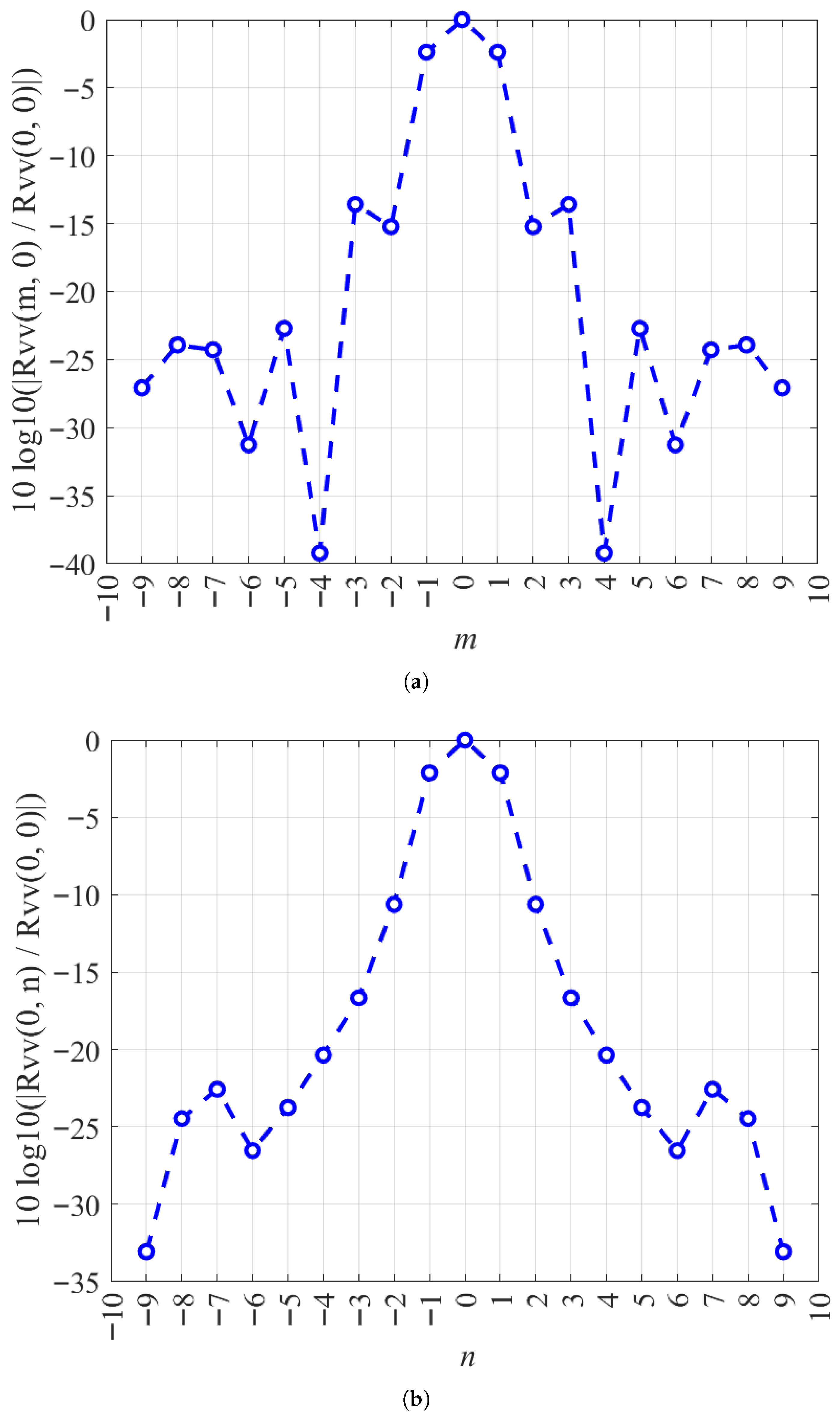
Figure 2 shows the estimated sequences of $R_{vv}(m,0)$ and $R_{vv}(0,n)$ for a HH-polarized SAR image acquired by the TerraSAR-X system over the Flevoland area in Netherlands. For determining the effective length of $R_{vv}(m,0)$ and $R_{vv}(0,n)$, we consider 20 dB as a threshold. We can see that when $\left|x\right|\ge 4,\left|y\right|\ge 4$, $10{log}_{10}\left[\right|R_{vv}(m,0)/R_{vv}(0,0)\left|\right]$ and $10{log}_{10}\left[\right|R_{vv}(0,n)/R_{vv}(0,0)\left|\right]$ will be less than −20dB. As a result, the effective length of $R_{vv}(m,0)$ and $R_{vv}(0,n)$ are both 7. Thus, we have $l_m=1$, $l_n=1$. This motivates us that the downsampling rate for such a SAR image should be $max\left(l_m,l_n\right)+1$, which is two for this TerraSAR-X image.

3.4.2. Mask Design

In the proposed Speckle2Self above, the generation of the mask is not specified, as long as the selected pixels are blinded. Here, we provide a set of regular designed masks to make the blinding operation more efficient, where the target pixels are selected at equal intervals. Denote by $m_{st}$ and $n_{st}$ the pixel step size in the row (m-) and column (n-) direction. The mask set consists of $m_{st}\times n_{st}$ masks. And the jth mask ${\mathit{b}}_{m_{st},n_{st}}^j$ is defined as (25) with the following positions $(u,v)$:

$$u=m_{st}{k}_1+j//n_{st},$$

(45)

$$v=n_{st}{k}_2+\mathrm{mod}(j,m_{st}),$$

(46)

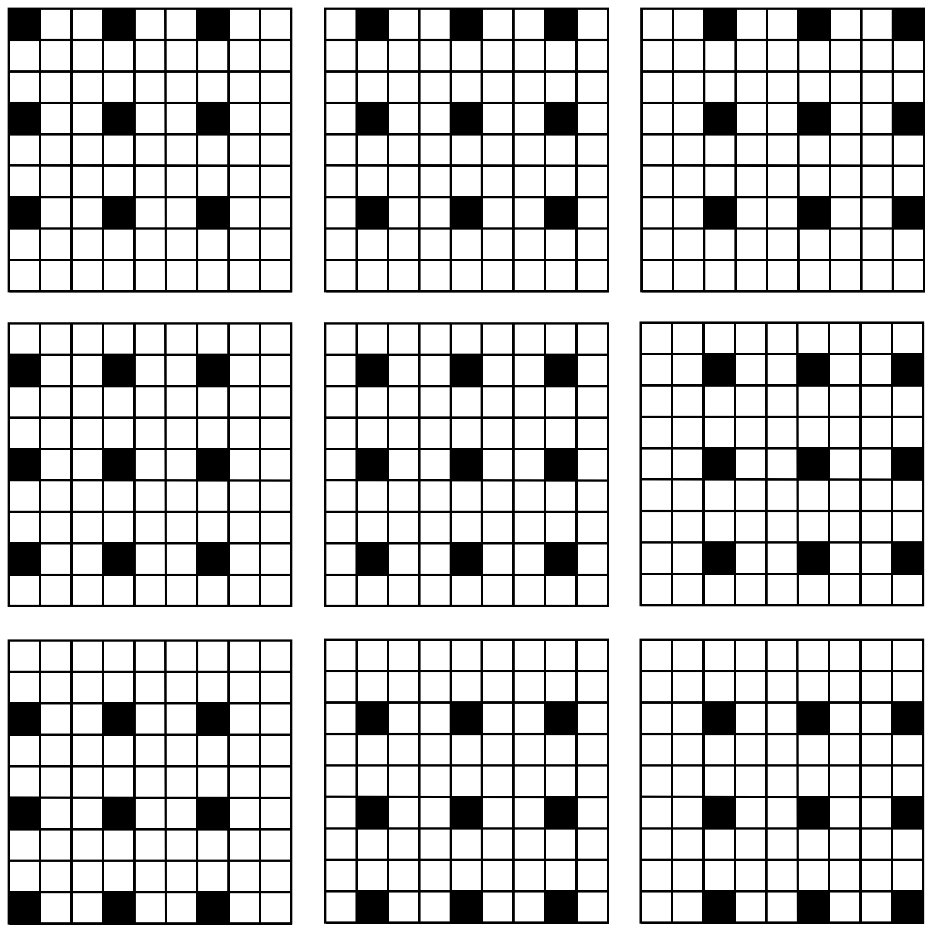
where $//$ represents taking the modulus, $\mathrm{mod}(·)$ represents taking the remainder, and $\forall k_1,k_2,s.t. 0\le u<H,0\le v<W.$ Figure 3 shows the designed mask set ${\left\{{\mathit{b}}_{3,3}^j\right\}}_{j=0}^{j=8}$ for an image with size of $9\times 9$. Any pixel value in the image can be blinded by the nine designed masks. For a given SAR image $\mathit{y}\in {\mathbb{R}}^{H\times W}$, the mask in the masking operation is selected randomly from the designed mask set

$${\left\{{\mathit{b}}_{m_{st},n_{st}}^j\right\}}_{j=0}^{j=m_{st}\times n_{st}-1}$$

(47)

where the set element is given by (25), (45) and (46).

3.4.3. Masked Loss Function

According to (25), the loss function in a vector form is defined as

$$\begin{array}{cc}\hfill \mathcal{L}\left(\mathit{y},\mathit{x}\right)=& \sum _{pixelwise}\left({\displaystyle \frac{{\left(\mathit{y}-\mathit{x}\right)}^2}{2}}+{\displaystyle \frac{{\left(\mathit{y}-\mathit{x}\right)}^3}{3!}}+\right.\hfill \\ \hfill & \left.{\displaystyle \frac{{\left(\mathit{y}-\mathit{x}\right)}^4}{4!}}+{\displaystyle \frac{{\left(\mathit{y}-\mathit{x}\right)}^5}{5!}}+{\displaystyle \frac{1}{\lambda }}\mathcal{F}\left(\mathit{x}\right)\right).\hfill \end{array}$$

where the power exponent of a vector or matrix is defined as the power exponent of each vector or matrix element, and the sum function ${\displaystyle \sum _{pixelwise}}\left(·\right)$ refers to summing each element of a vector or matrix.

In our training scheme, the proposed network predicts the masked pixel only. Hence, the loss function in our training scheme is expressed in a masked form:

$$\mathcal{L}\left(\mathit{y}\odot \overline{\mathit{b}},{\mathit{x}}_{pred}\odot \overline{\mathit{b}}\right),$$

(48)

where ⊙ denotes the element-wise multiplication, $\overline{\mathit{b}}$ is the complementary mask defined in (31), $\mathit{y}$ is the noisy image, and ${\mathit{x}}_{pred}$ is the despeckled image predicted by our network.

3.5. Despeckling Scheme

The trained NN predicts the masked pixel values indicated by the designed mask for despeckling. Since any pixel in the image can be blinded by the nine designed masks without duplication, we can achieve the despeckling of all pixels of the entire image by using the trained network to predict the masked images given by the whole designed mask set. Denote by ${\mathcal{F}}_{\theta }$ the trained network with weight parameters $\mathit{\theta }$, which means ${\mathit{x}}_{pred}={\mathcal{F}}_{\theta }\left(\mathit{y},\mathit{b},\overline{\mathit{b}}\right)$. We have

$${\mathit{x}}^{\ast }=\sum _{\mathit{b}}{\mathcal{F}}_{\theta }\left(\mathit{y},\mathit{b},\overline{\mathit{b}}\right)\odot \overline{\mathit{b}},$$

(49)

where $\mathit{b}\in {\left\{{\mathit{b}}_{m_{st},n_{st}}^j\right\}}_{j=0}^{m_{st}\times n_{st}-1}$, and ${\mathit{x}}^{\ast }$ is the despeckled result for the NN input log-transformed SAR image $\mathit{y}$.

It should be pointed out that the input SAR image $\mathit{y}$ is a downsampled image for whitening consideration. Of course, if whitening downsampling is not required, (49) is the final result. Otherwise, for a full-resolution input image ${\mathit{y}}_{full}$, we downsample it with a given downsampling rate r into sub-images ${\mathit{y}}_1,\dots ,{\mathit{y}}_{r^2}$. For the ith sub-image ${\mathit{y}}_i$, (49) can be rewritten as

$${\mathit{x}}_i^{\ast }=\sum _{\mathit{b}}{\mathcal{F}}_{\theta }\left({\mathit{y}}_i,\mathit{b},\overline{\mathit{b}}\right)\odot \overline{\mathit{b}},$$

(50)

where ${\mathit{x}}_i^{\ast }$ is the ith despeckled sub-image. Based on all the $r^2$ despeckled sub-images, we can recover the full-resolution despeckled image ${\mathit{x}}_{full}^{\ast }$ in an opposite way of the downsampling above. The full-resolution image ${\mathit{x}}_{full}^{\ast }$ is exactly the final despeckled result for the full-resolution input image ${\mathit{y}}_{full}$. The entire despeckling scheme is summarized in Algorithm 1.

Algorithm 1 Speckle2Self Despeckling Scheme

Input: SAR image ${\mathit{y}}_{full}$, mask step size $m_{st}$ and $n_{st}$,

Downsampling rate r, trained NN ${\mathcal{F}}_{\theta }$.

Output: Despeckled result ${\mathit{x}}_{full}^{\ast }$.

1: /*Mask Generation*/   2: Generate a set of regular masks ${\left\{{\mathit{b}}_{m_{st},n_{st}}^j\right\}}_{j=0}^{m_{st}\times n_{st}-1}$ based on (25), (45) and (46).   3: /*Image Downsampling*/   4: Downsample the SAR image ${\mathit{y}}_{full}$ with rate r: ${\mathit{y}}_1,\dots ,{\mathit{y}}_{r^2}$.   5: repeat   6:    Select one sub-testimage ${\mathit{y}}_i$ without duplication.   7:    /*Initialization*/   8:    ${\mathit{x}}_i^{\ast }=0$.   9:    /*Image Despeckling*/ 10:    for $j=0$ to $m_{st}\times n_{st}-1$ do 11:        Choose $\mathit{b}={\mathit{b}}_{m_{st},n_{st}}^j$. 12:        Predict ${\mathit{x}}_{pred}={\mathcal{F}}_{\theta }\left({\mathit{y}}_i,\mathit{b},\overline{\mathit{b}}\right)$. 13:        ${\mathit{x}}_i^{\ast }={\mathit{x}}_i^{\ast }+{\mathit{x}}_{pred}\odot \overline{\mathit{b}}$. 14:     end for 15: until All despeckled sub-images ${\mathit{x}}_1^{\ast },\dots {\mathit{x}}_{r^2}^{\ast }$ are obtained. 16: /*Image Upsampling*/ 17: Upsample the sub-images ${\mathit{x}}_1^{\ast },\dots {\mathit{x}}_{r^2}^{\ast }$ to ${\mathit{x}}_{full}^{\ast }$ in an opposite way of the above downsampling.

4. Experiments and Results

4.1. Parameter Settings and Experimental Details

The algorithm parameter settings are summarized in

Table 1. Algorithm parameter settings.

Algorithm Parameters	Symbols	Values
Full Image Size	$\mathcal{H}\times \mathcal{W}$	$448\times 448$
Downsampling Rate	r	2
Downsampled Image Size	$H\times W$	$224\times 224$
Patch size	P	16
Number of Patches	N	196
Embedding Feature Dimension	D	768
Encoder Depth	$Loe$	12
Decoder Depth	$Lod$	2
Mask Interval in Row Direction	$m_{st}$	3
Mask Interval in Column Direction	$n_{st}$	3

. The input image size of full resolution is $448\times 448$. According to the downsampling criterion mentioned in Section 3.4, the downsampling rate is set as 2, which is effective and sufficient for variety of sensor images in experiments, such as Radarsat-2, ALOS-2, TerraSAR-X and GaoFen-3. Hence, the size of the downsampled image as input to the network is $224\times 224$. The parameters for the network, such as patch size, embedding dimension, and encoder depth, is consistent with the basic parameters of the Transformer-series network. As for mask design, the mask intervals in the row and column directions are set as 3 and corresponding visualization can be found in Figure 3.

In the training process, the weight parameters of the network are initialized by Kaiming Initialization [79]. The batch size is set as 64. The basic learning rate is 2.5 × 10⁻⁴ with 10 epochs for warming up, and the learning rate decreases in cosine schedule. The network is trained for a total of 200 epochs. The SGD optimizer is employed for our experiments, with a weight decay of 0.05. Data augmentation operations include random rotation and random flip. The proposed algorithm is implemented in the Pytorch framework and trained on a server equipped with Ubuntu 20.04, Intel Xeon Gold 6226R processor, 520-GB RAM, and eight Nvidia GeForce RTX 3090 GPUs.

4.2. Training Datasets and Test Images

A synthetic image dataset and a real image dataset are constructed for performance evaluation. The simulated images are synthesized based on natural images and synthetic speckle noise. In classic speckle models, the fully developed speckle is multiplicative and follows a gamma distribution. We select clean images from the Berkeley Segmentation Dataset (BSD), generate random variables as speckle noise, and combine them with multiplication to produce synthetic images. In total, 450 different images from BSD form a training dataset. Several typical images, such as the Monarch and Pepper, are selected for testing, including visualization comparison and quantitative assessment.

For the real image dataset, we employ TerraSAR-X images via the download link provided by [69]. Since the TerraSAR-X images are single-look data, in order to increase the data diversity, images acquired by AIRSAR, RADARSAT-2, and GaoFen-3 are also added to our dataset. Various geographical regions and landcover types are studied in the dataset. These large scene images are sliced into patches of size $448\times 448$. The authors in [69] also provide five TerrSAR-X test images. We selected one of the images (denoted as Image-5) to directly compare our method with reference methods. Furthermore, another four real images taken over Netherlands—Flevoland; China—Dalian; Singapore; and USA—San Francisco are also used. These four images are acquired by AIRSAR, TerraSAR-X, RADARSAT-2, and GaoFen-3, respectively.

4.3. Reference Methods and Evaluation Metrics

4.3.1. Reference Methods

In order to validate the proposed method, experiments have been carried out on both simulated and real data. Between the available approaches, we consider PPB [24], SAR-BM3D [29], ID-CNN [36], and Speckle2Void [69] as reference methods for comparison with our proposed networks. For PPB, SAR-BM3D, and Speckle2Void, we use the code implementation of the authors. ID-CNN has been implemented from scratch, adhering strictly to the guidelines specified in the original paper regarding CNN architecture and hyperparameters. For each method, the parameters have been set according to those suggested in the relative articles. Note that PPB, SAR-BM3D, and ID-CNN are supervised methods, while Speckle2Void is a neural network-based method with self-supervised training. Similarly to Speckle2Void, we do not directly compare with the recent works in [67,68], as they use multi-temporal data for groundtruth generation or as pseudo-label, which would make the setting unfair with respect to the single observation of a scene in our case.

4.3.2. Evaluation Metrics

Considering that the groundtruth of the synthetic image data exists, we use the peak signal-to-noise ratio (PSNR) and the structural similarity (SSIM) to achieve performance evaluation on the synthetic dataset. PSNR allows us to gain a quantitative understanding of the denoising capabilities of our network and other comparative methods. As a supplement to PNSR, SSIM mainly evaluates the recovery performance of image structural information.

In terms of the real-image dataset, several reference-free performance metrics, including equivalent number of looks (ENLs) and moments of the ratio image $({\mu }_r,{\sigma }_r)$, are employed for performance comparison between the proposed method and the reference methods. The ENL is commonly estimated by identifying homogeneous regions in an image, where the speckle is fully developed and contribution of texture is negligible, meaning that the radar cross-section is assumed to be constant [80]. The ENL is estimated over apparently homogeneous areas in the image. For single-channel images, the ENL is defined as the ratio of the square average intensity to the variance. The ratio image is defined as the pixel-wise ratio of the original image to the denoised image.

Moments of the ratio image measure how close the obtained ratio image is to the statistics of pure speckle. The mean ${\mu }_r$ and variance ${\sigma }_r$ of the ratio image indicate the bias and speckle power suppression, respectively. It is desirable for the mean of the ratio image to be as close to 1 as possible. The variance of the ratio image should be close to the reciprocal of the number of looks.

4.4. Results with Synthetic Images

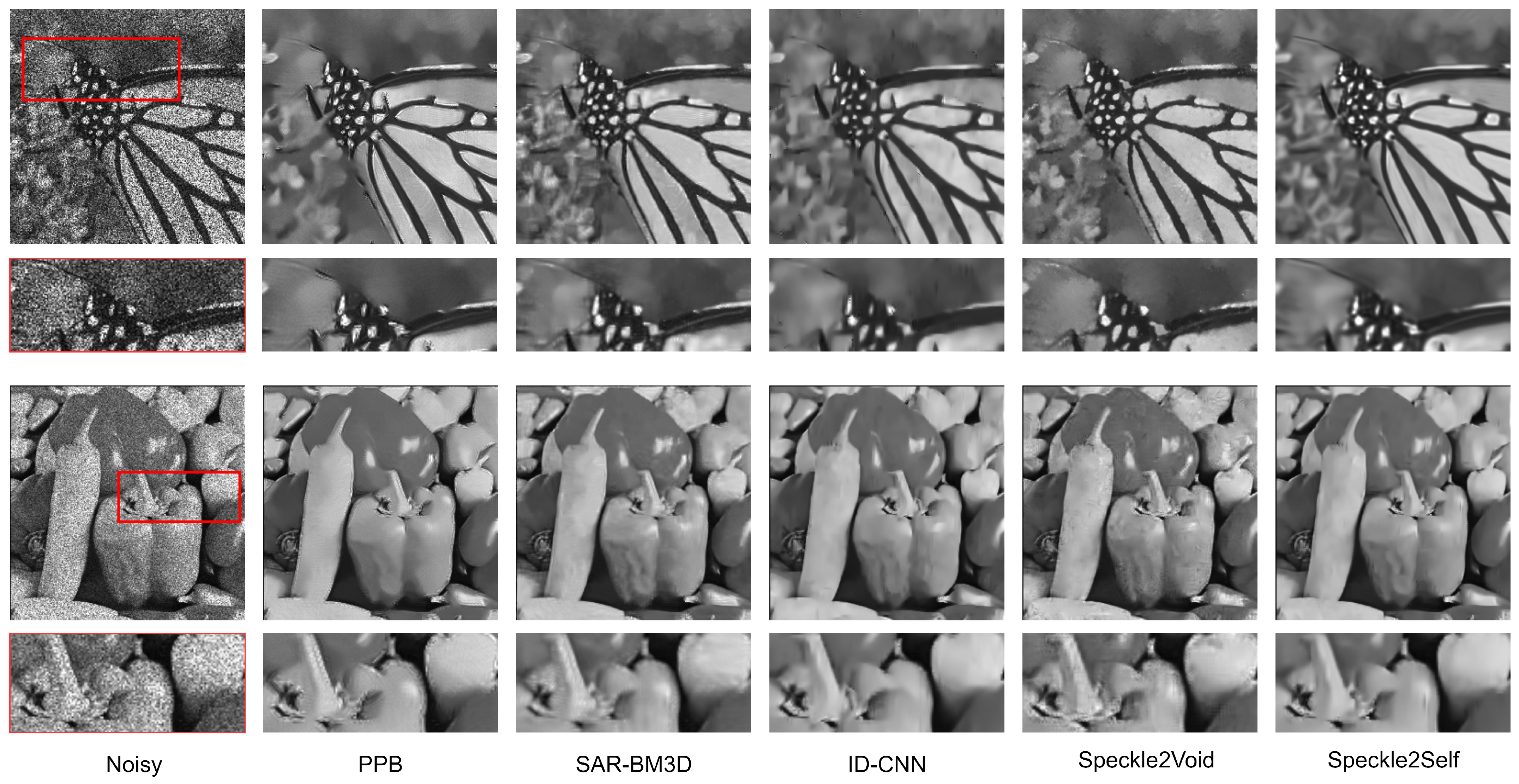
Figure 4 presents the despeckled results of the proposed method and reference methods for the Monarch (top two rows) and Pepper (bottom two rows). The ENL of the noisy images for the Monarch and Pepper are 1 and 4, respectively. The second and fourth rows are enlarged views of the areas in the red boxes in the first and third rows of images, respectively. It can be seen that obvious marks are produced on the edge of the pepper in the despeckled results of PPB and Speckle2Void. In addition, SAR-BM3D, ID-CNN, and the proposed Speckle2Self all have better speckle suppression and detail retention capabilities, and at the same time, produce fewer artifacts. Similar results can also be observed in the results for the Monarch, especially in the tentacle area of the Monarch.

Table 2. PSNR (dB) on the Despeckled Synthetic Images. The best results are emphasized in boldface.

		PPB	SAR-BM3D	ID-CNN	Speckle2Void	Speckle2Self
Monarch	$L=1$	22.74	24.58	23.23	23.15	24.26
	$L=2$	24.27	26.29	26.35	25.67	26.07
	$L=4$	26.02	28.63	28.70	27.96	28.41
	$L=8$	27.39	29.73	29.27	28.94	29.91
	$L=16$	28.93	30.35	30.02	29.97	30.60
Peppers	$L=1$	23.86	24.91	24.06	23.24	24.58
	$L=2$	25.50	26.56	26.40	25.71	26.93
	$L=4$	26.95	27.90	28.27	27.36	28.11
	$L=8$	28.43	29.72	29.04	28.88	30.67
	$L=16$	29.86	31.37	30.63	30.62	31.33

and

Table 3. SSIM on the despeckled synthetic images. The best results are emphasized in boldface.

		PPB	SAR-BM3D	ID-CNN	Speckle2Void	Speckle2Self
Monarch	$L=1$	0.713	0.790	0.752	0.754	0.787
	$L=2$	0.778	0.843	0.845	0.819	0.841
	$L=4$	0.837	0.891	0.890	0.874	0.904
	$L=8$	0.871	0.915	0.914	0.905	0.925
	$L=16$	0.903	0.922	0.920	0.912	0.917
Peppers	$L=1$	0.678	0.747	0.698	0.626	0.737
	$L=2$	0.739	0.798	0.779	0.725	0.788
	$L=4$	0.790	0.824	0.830	0.796	0.838
	$L=8$	0.831	0.872	0.843	0.839	0.877
	$L=16$	0.865	0.897	0.901	0.873	0.896

present the PSNR and SSIM on the despeckled images of the test methods for the Monarch and Pepper. The best results are emphasized in boldface. We can see that SAR-BM3D and ID-CNN perform the best among the supervised methods. Compared with Speckle2Void, the proposed Speckle2Self has considerable improvements in PSNR and SSIM. It is worth mentioning that the proposed Speckle2Self outperforms PPB for all ENL settings and has comparable performance with respect to SAR-BM3D and ID-CNN, which are all supervised despeckling methods. Despite the absence of the true clean images during training, the proposed method achieves good noise suppression and detail–content preservation. Whether in terms of visualization comparison or quantitative evaluation, the performance of Speckle2Self is equivalent to those of the traditional state-of-the-art method SAR-BM3D and the CNN baseline method ID-CNN and is significantly better than that of Speckle2Void.

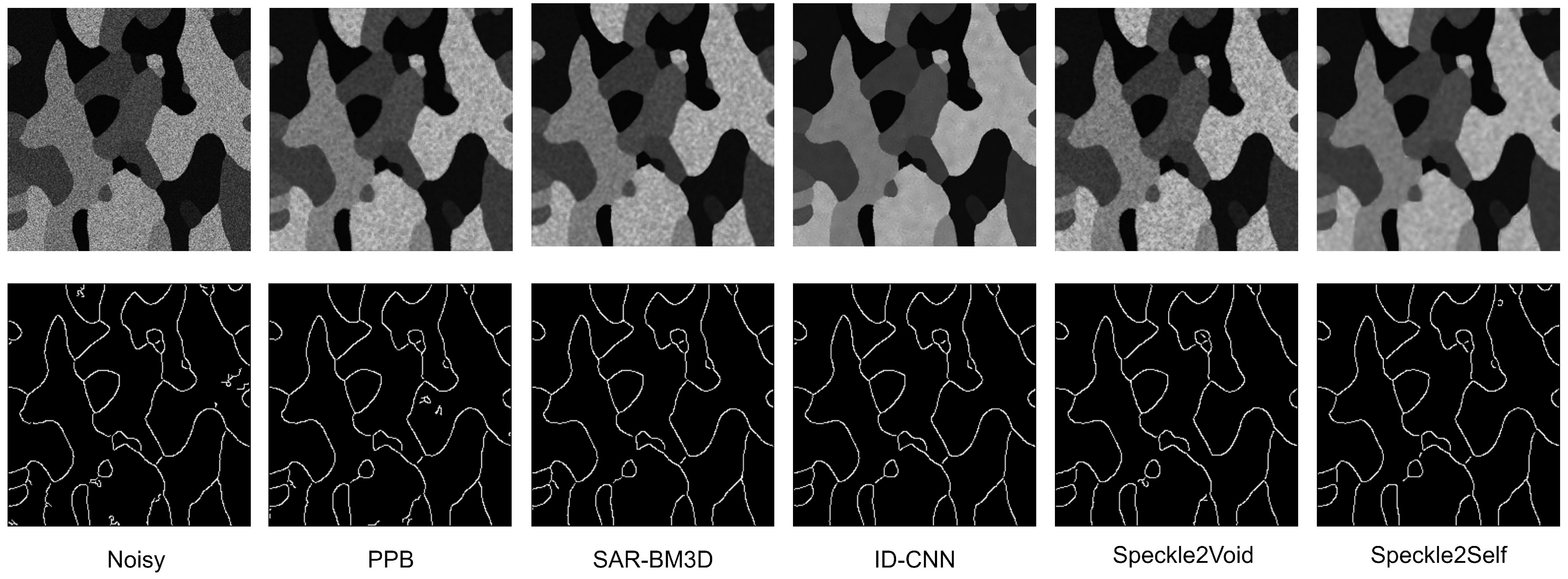
To further assess the influence of different filtering methods on edge-detection performance, we conducted a Monte Carlo simulation experiment. Seven uniform regions were selected from the Netherlands—Flevoland SAR image and corresponding homogeneous regions were generated using their regional means. Noisy pixels were then simulated using the Monte Carlo procedure. The top row of Figure 5 shows the simulated image with $L=2$ and the corresponding despeckled results. The proposed Speckle2Self demonstrates strong speckle suppression while effectively preserving structural details. Although Speckle2Void also suppresses speckle, it introduces noticeable edge blurring.

To evaluate edge preservation, the Canny operator was applied to both the noisy and filtered images, with the results shown in the bottom row of Figure 5. PPB and Speckle2Void produce numerous false edges in homogeneous areas. The proposed method and SAR-BM3D reduce these artifacts but still introduce slight blurring in some fine structures.

Table 4. Boundary F1-scores of the Canny edge-detection results (bottom row of Figure 5). The best results are emphasized in boldface.

PPB	SAR-BM3D	ID-CNN	Speckle2Void	Speckle2Self
92.93	94.55	94.87	93.48	95.12

summarizes the Boundary F1-scores computed from the Canny detection results. Speckle2Self achieves the highest score (95.12), confirming its superior ability to balance speckle suppression and structural-detail preservation.

4.5. Results with Real Images

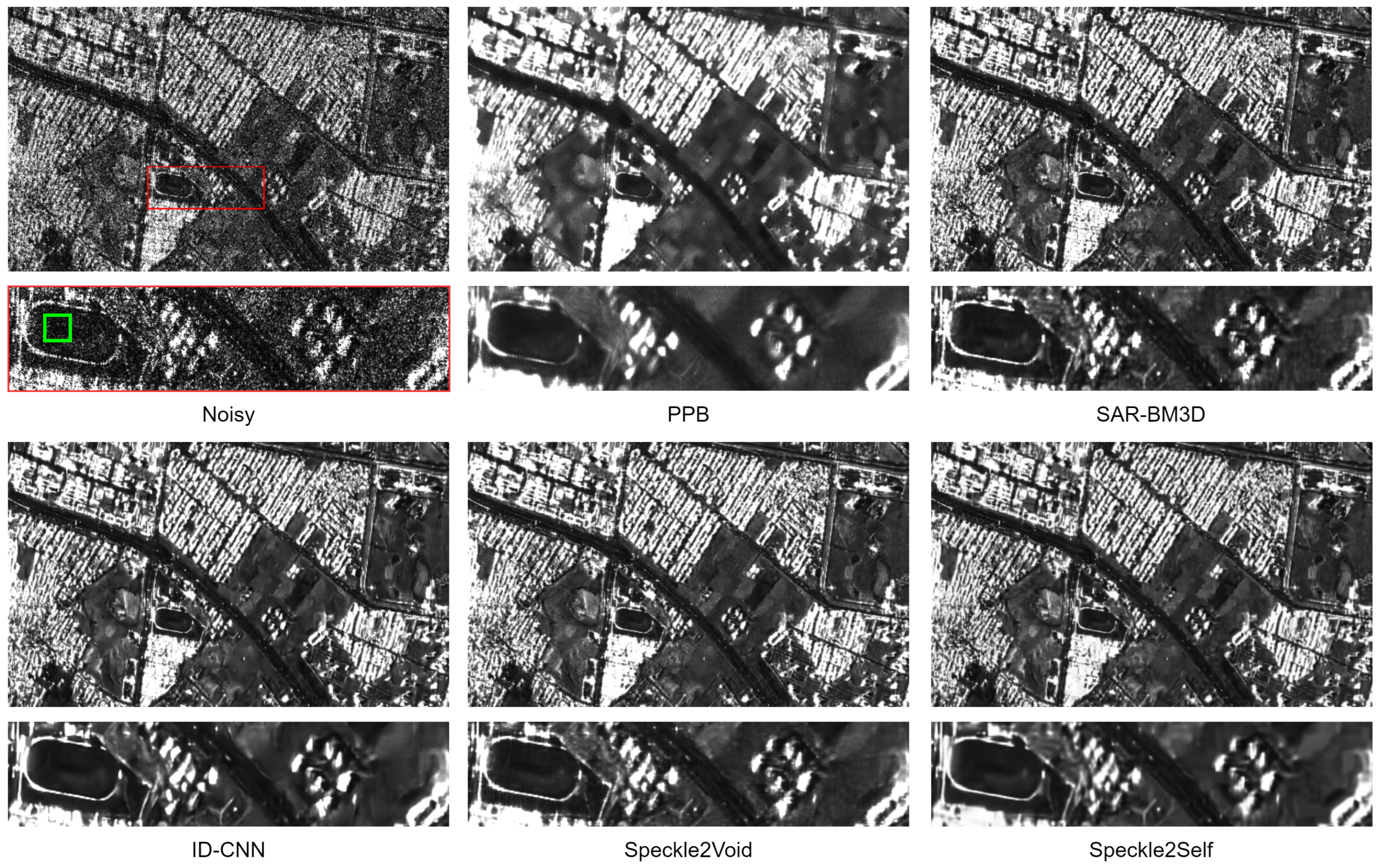
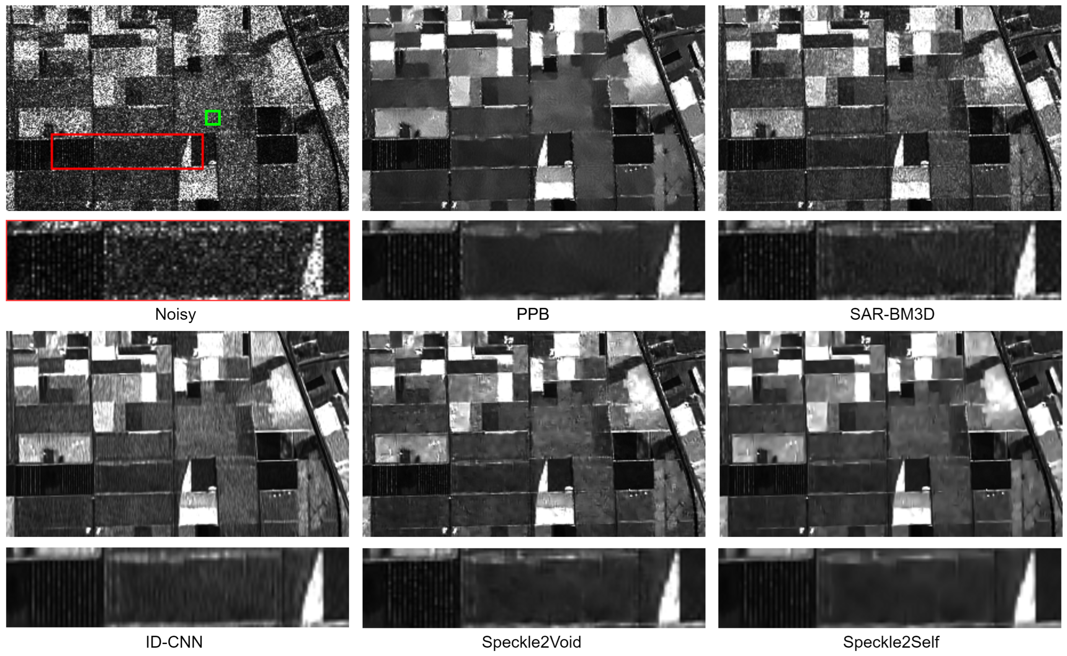
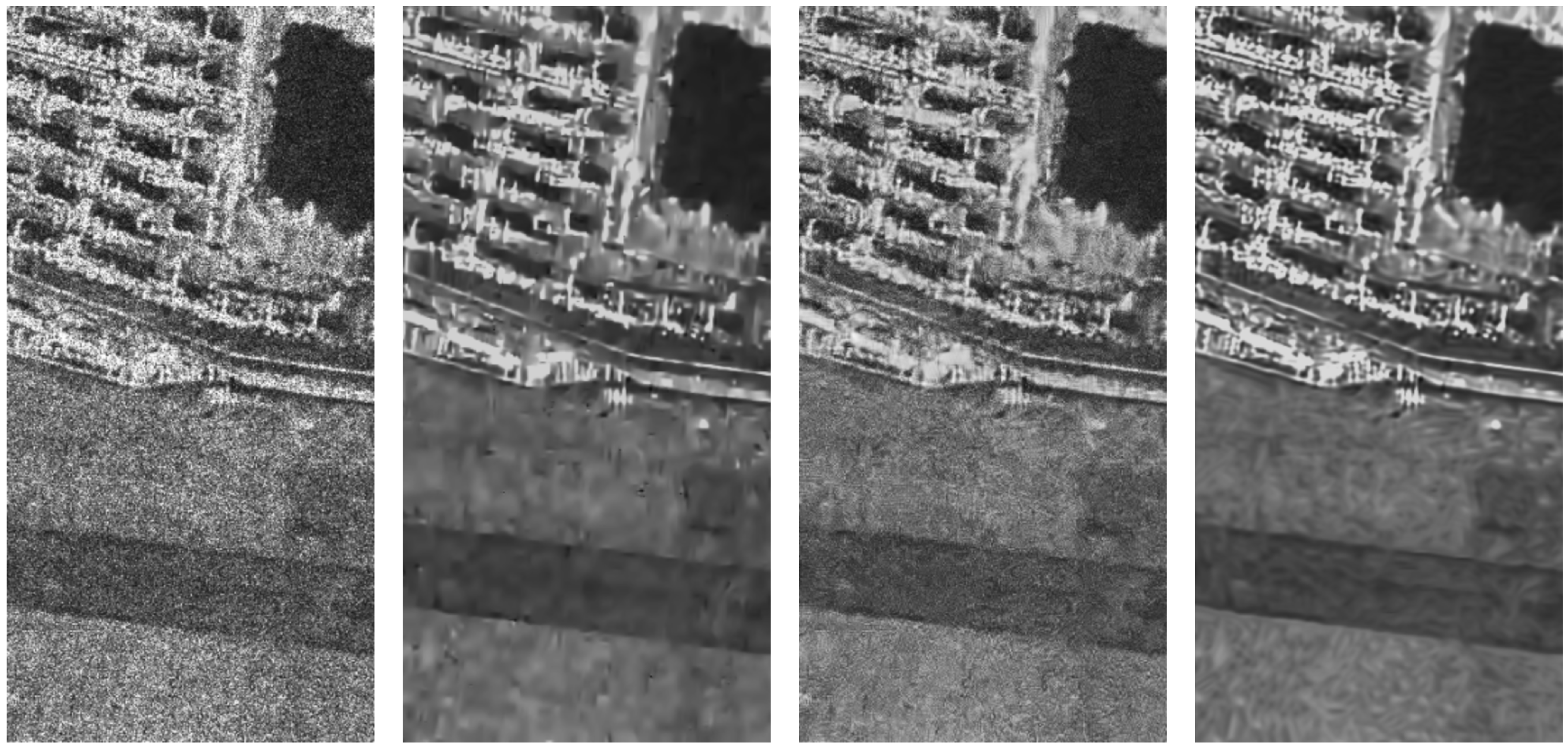
In order to evaluate the despeckling performance of the test methods on real images, we used real images as the input and presented the denoised results for comparison. Figure 6 and Figure 7 show the despeckled results for the Image-5 in [69] and Flevoland. The ENL of the noisy images for these two are $0.87$ and $2.99$, respectively. In each subfigure of both Figure 6 and Figure 7, the top row depicts the overview of the despeckled result and the bottom row presents the local details of the area marked by the red box in the top row. We can see that the result of PPB has the best noise suppression effect and the smoothest picture, but it also loses a lot of details. SAR-BM3D has better ability to maintain details in urban areas, but its ability to suppress speckle noise is much inferior to that in synthetic images. This is because the coherence spots of measured SAR images are spatially correlated, and SAR-BM3D was proposed on the basis of spatially non-correlated noise. The despeckled results of ID-CNN show great speckle suppression, but meanwhile, tend to over-smooth and produce cartoon-like edges, which was mentioned and verified in [69]. In addition, in the detail close-up of Figure 7, we can observe obvious longitudinal anomaly patterns in the flat areas of the ID-CNN results. Speckle2Void produces relatively higher quality images. However, certain artifacts can be seen in the intersection areas of different landcovers in Figure 7 for Flevoland. Contrary to other methods, Speckle2Self avoids introducing artifacts in homogeneous regions, yielding images of superior quality. Compared with alternative reference methods, it generates more realistic details, particularly in texture-rich areas with artificial structures.

We list the metrics for the real-image evaluation in

Table 5. ENL of the despeckled images and moments of corresponding ratio images. The best results are emphasized in boldface.

	Image-5 [69] ($\mathit{L}=0.87$)			Dalian ($\mathit{L}=1.02$)			Flevoland ($\mathit{L}=2.99$)
	ENL	${\mathit{\mu }}_{\mathit{r}}$	${\mathit{\sigma }}_{\mathit{r}}$	ENL	${\mathit{\mu }}_{\mathit{r}}$	${\mathit{\sigma }}_{\mathit{r}}$	ENL	${\mathit{\mu }}_{\mathit{r}}$	${\mathit{\sigma }}_{\mathit{r}}$
PPB	22.93	0.85	0.89	42.49	0.93	0.79	148.91	0.97	0.25
SAR-BM3D	16.24	0.89	0.55	8.98	0.90	0.53	40.83	0.95	0.19
ID-CNN	16.61	0.92	0.66	22.27	0.92	1.69	79.22	0.89	0.31
Speckle2Void	18.90	0.95	0.75	31.46	0.91	0.82	92.85	0.93	0.29
Speckle2Self	19.03	0.96	0.83	46.83	0.97	0.97	133.08	0.99	0.34

, including the ENL of the despeckled images and the moments of corresponding ratio images. The number of looks of the noisy images are marked as L in the first row of Table 5. It can be easily seen that PPB achieves the highest ENL on almost all the three images, which is consistent with the results of visualization comparison in Figure 6 and Figure 7. In terms of the moments of the ratio images, as mentioned in Section 4.3, the mean and ENL of the ratio image of a good despeckling result should be as close as possible to the mean and ENL of the real speckle. Thus, we can see that the proposed Speckle2Self outperforms the reference methods significantly.

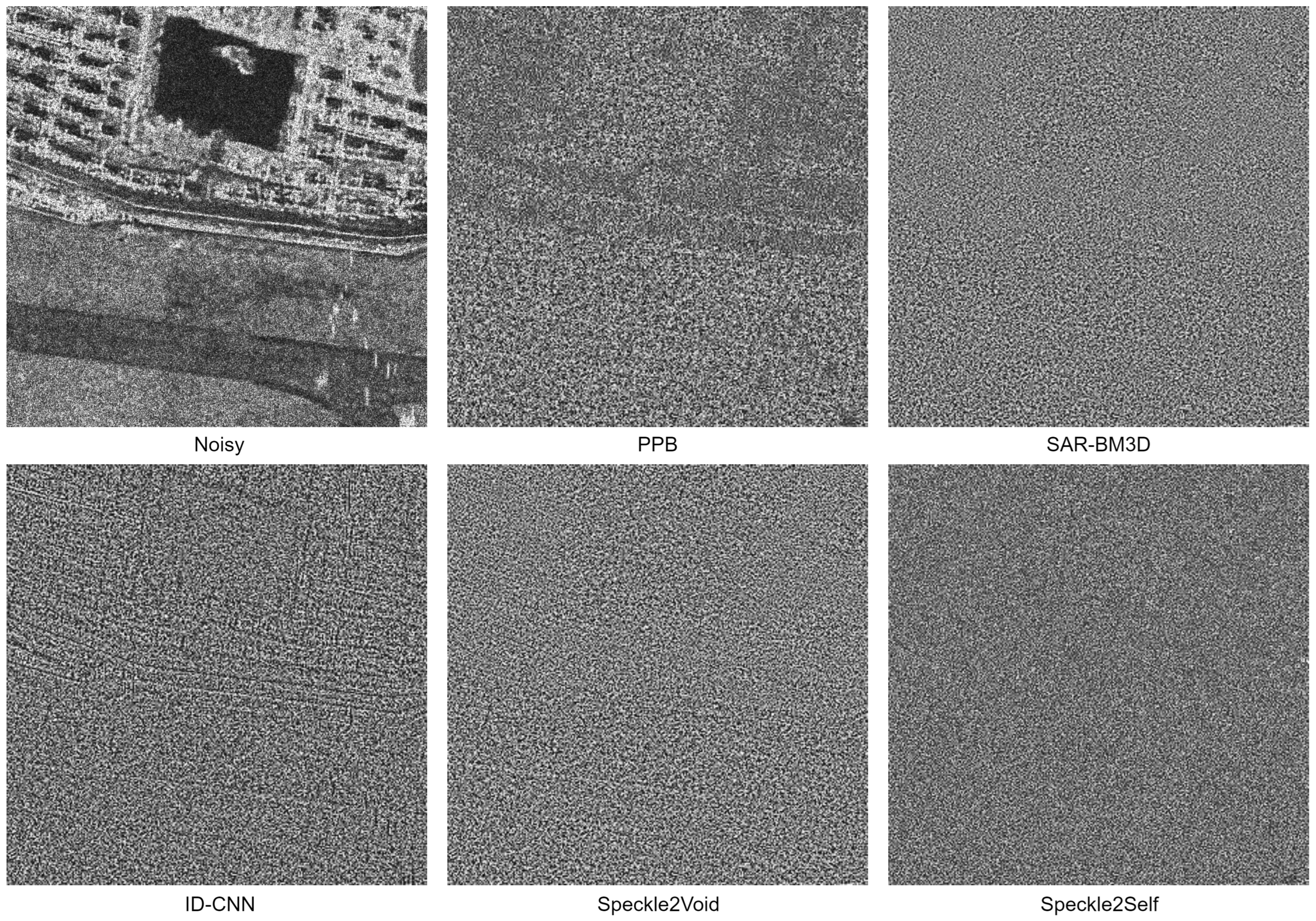
Figure 8 presents the ratio images for Dalian between the noisy and despeckled images. Ideally, no structure should be evident in the ratio images. Obvious low-brightness dark-spot structures can be seen in the ratio image of PPB, while obvious linear edges can be observed in the ratio image of ID-CNN, especially in urban areas. There are fewer structures but still certain heterogeneous lines in the results of SAR-BM3D and Speckle2Void. And we can observe the capability of our proposed Speckle2Void to remove the speckle effectively, with a minimal amount of visible artifacts and patterns.

4.6. Model Complexity and Time Consumption

To assess computational efficiency, we compare the model complexity and runtime of several representative despeckling methods.

Table 6. Quantitative comparison of model complexity in terms of the number of parameters as well as training and inference time consumption per sample.

Method	PPB	SAR-BM3D	ID-CNN	Speckle2Void	Speckle2Self
Parameters (M)	-	-	2.03	5.34	7.95
Execution Time per Sample
for Training (s)	-	-	0.084	0.096	0.097
Execution Time per Sample
for Inference (s)	13.39	38.47	0.076	0.088	0.090

reports the number of trainable parameters and the average execution time per sample for both training and inference. While model-based methods (PPB and SAR-BM3D) require substantial inference time due to iterative procedures, the learning-based methods exhibit significantly faster runtimes. The proposed Speckle2Self, despite having a larger parameter count (7.95 M), achieves training and inference speeds comparable to Speckle2Void, indicating that the introduction of attention mechanisms does not impose excessive computational burden.

4.7. Comparison with Speckle2Void

The reference methods all are supervised despeckling approaches, except Speckle2Void. From the evaluations in Section 4.3 and Section 4.4, we can clearly see that the proposed Speckle2Self achieves comparable performance at least to the supervised method, and significant improvements are obtained when compared with Speckle2Void.

Besides the evaluation metrics used above, blind despeckling is also an important issue. The supervised filters as well as Speckle2Void are non-blind filters, which require prior knowledge of the noise level. The ENL of the noisy image often acts as an input parameter for these filters. Inappropriate parameter settings will degrade filter performances. The blind denoising issue for the supervised methods has been discussed in [81]. Hence, here, we choose Speckle2Void for comparison in terms of blind denoising.

For a noisy SAR image pixel $y_i$, Speckle2Void employs a CNN to estimate the parameters ${\alpha }_i$ and ${\beta }_i$ of a prior distribution of the speckle. The despeckled image pixel is obtained through a MMSE estimator combining a likehood distribution:

$$p(y_i|y_i^{R{F}_j\setminus j})={\displaystyle \frac{L^L{y}_i^{L-1}}{{\beta }_i^{-{\alpha }_i}\mathrm{Beta}\left(L,{\alpha }_i\right){\left({\beta }_i+L{y}_i\right)}^{L+{\alpha }_i}}},$$

(51)

where L denotes the ENL of the noisy image and $\mathrm{Beta}(·)$ denotes the beta function. The final despeckled pixel value is given by

$$x_{pred}={\displaystyle \frac{{\beta }_i+L{y}_i}{L+a_i-1}}.$$

(52)

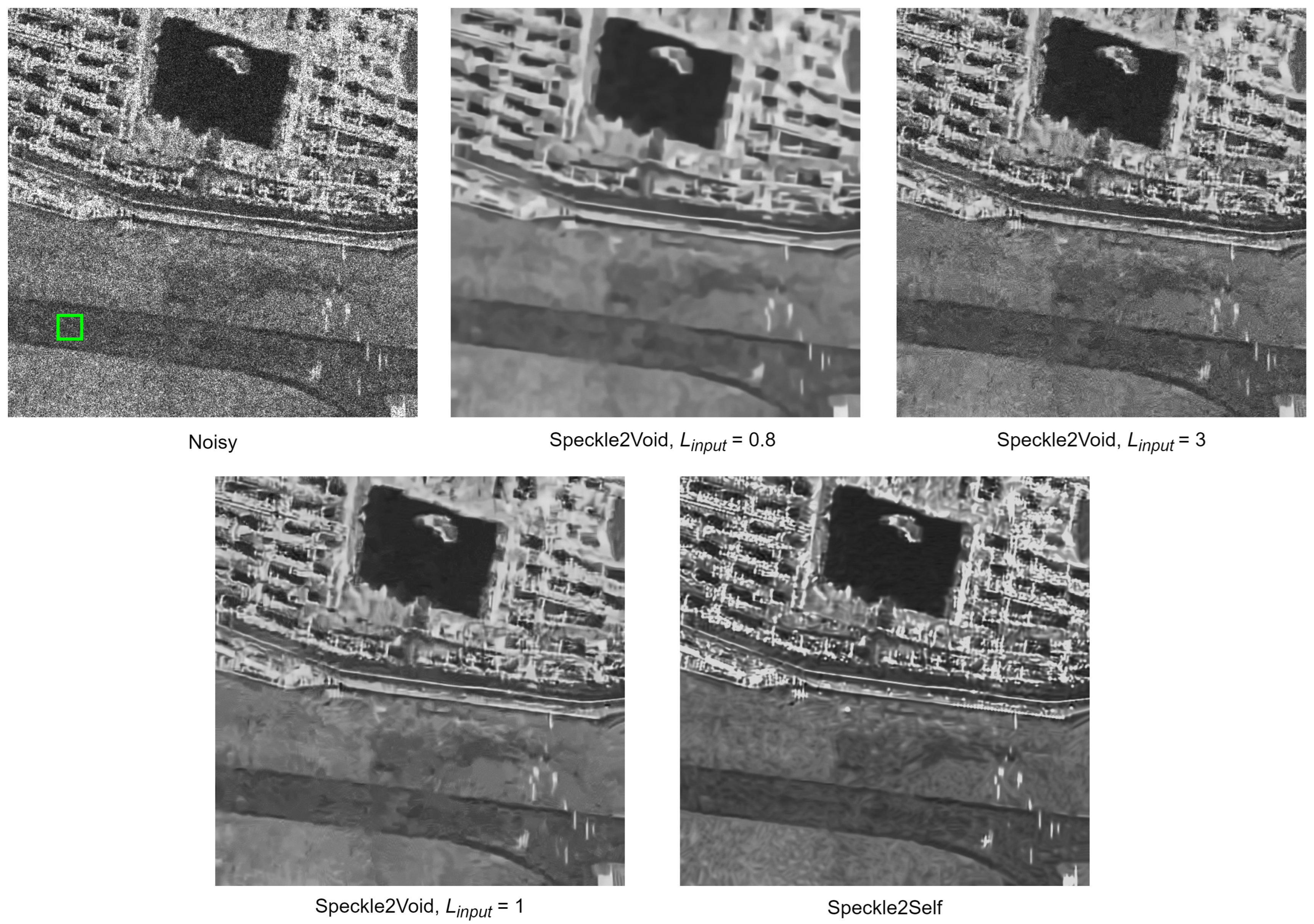
Obviously, we can see that the despeckled value $x_{pred}$ depends on the estimated parameters ${\alpha }_i$, ${\beta }_i$, and the ENL of the noisy image, which reflects the noisy level. The despeckling performances of Speckle2Void is highly related to the input of ENL. Inappropriate ENL settings would severely degrade the despeckling performances of Speckle2Void. Figure 9 shows the despeckled comparison between Speckle2Void with different inputs of ENL, and the proposed Speckle2Self. We can see that setting ENL below its actual value ($L_{input}=0.8$) would smooth out the details while removing the noise, and a too-high ENL setting ($L_{input}=3$) will bring about the problem of insufficient noise removal. Only when the ENL input is very close to the real ENL of the noisy image can Speckle2Void output relatively high-quality denoising results. On the contrary, the proposed Speckle2Self is an end-to-end despeckling approach and does not rely on inputting a prior ENL parameter. By only inputting a noisy SAR image, Speckle2Self produces a final despeckled result that suppresses noise in homogeneous areas and preserve details in structured areas.

4.8. Ablation Study

In the following, we discuss ablation studies in loss function, image downsampling, and regularizer.

4.8.1. Loss Function

In this paper, going one stop further of Noise2Void, we derive a novel loss function based on the statistics of SAR images in MAP framework, which takes the form of (25). The $l_2$ loss and $l_1$ loss are commonly used loss functions. Thus, we replace the proposed loss function with $l_2$ loss and $l_1$ loss for network training, and then use the trained networks for image despeckling. Figure 10 shows the despeckled results using different loss functions. We can see that $l_2$ loss function tends to guide our network to produce blurry images, where structured details are smoothed out too much and artifacts appear. In addition, more residual speckle in the denoised image of using $l_1$ loss can also be observed. In optical image denoising tasks, $l_2$ loss often corresponds to the median statistic, and $l_1$ corresponds to the mean statistic. We find that both loss functions are not optimal for SAR image despeckling. The result on Speckle2Void shows that the proposed loss function is able to achieve stronger speckle suppression while preserving details.

4.8.2. Image Downsampling

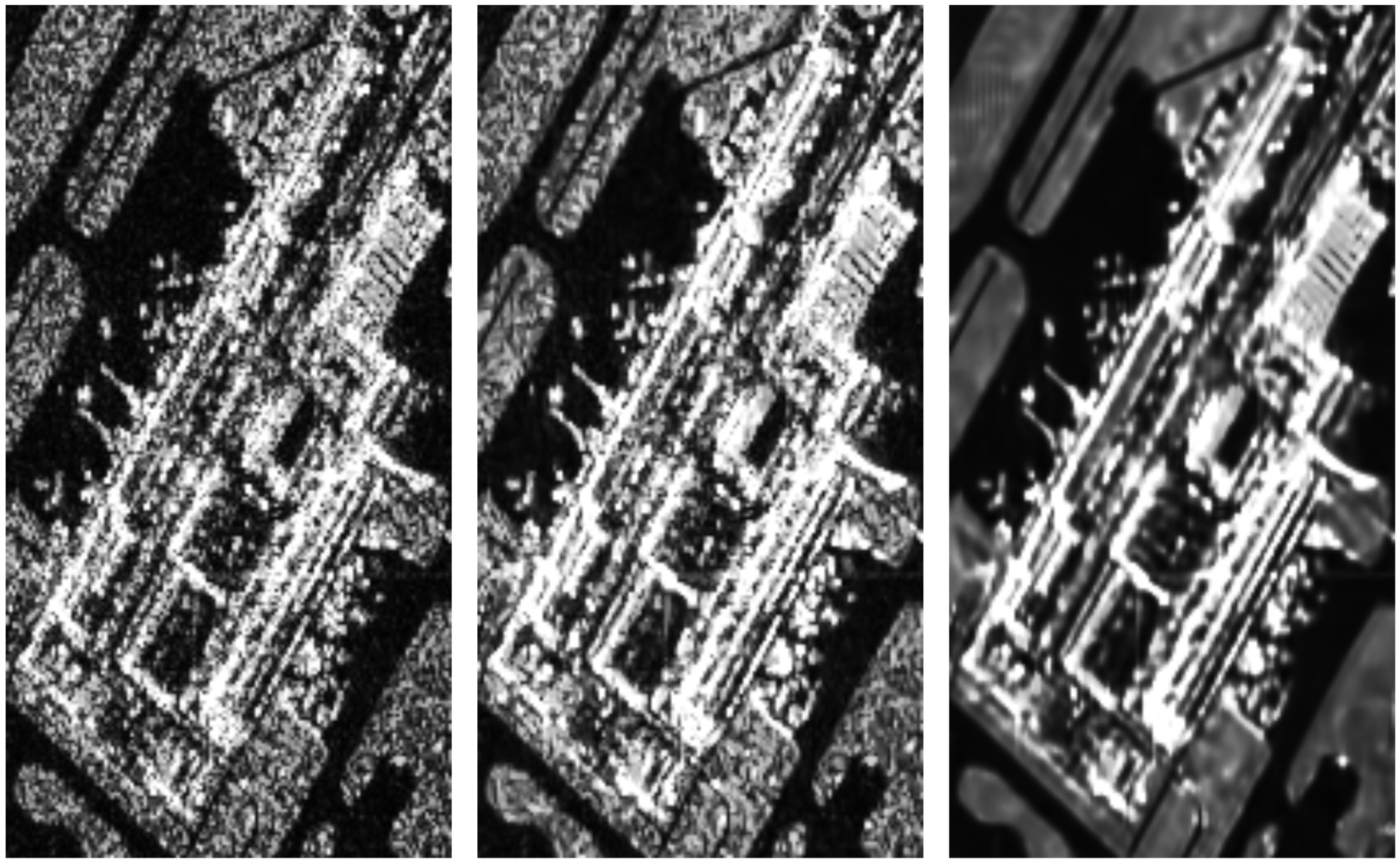
Due to the imaging mechanism of the SAR system, the speckle of SAR images is spatially correlated. We propose to use image downsampling for noise whitening. In order to verify the effectiveness of the image downsampling operation, we use non-downsampling data to training the network, generate despeckled results with the trained network, and compare them with those produced by our Speckle2Self using image downsampling. Figure 11 reports the despeckled results for the part of Singapore with and without image downsampling. Comparing the middle and right images, we can find that no image downsampling will result in serious insufficient noise filtering. Our derivation in (19) is based on the noise-whitening assumption. And noise without whitening will cause our derivation to fail. Hence, we can conclude that image downsampling is quite necessary for image downsampling, and improves despeckling performance significantly.

4.8.3. Regularizer

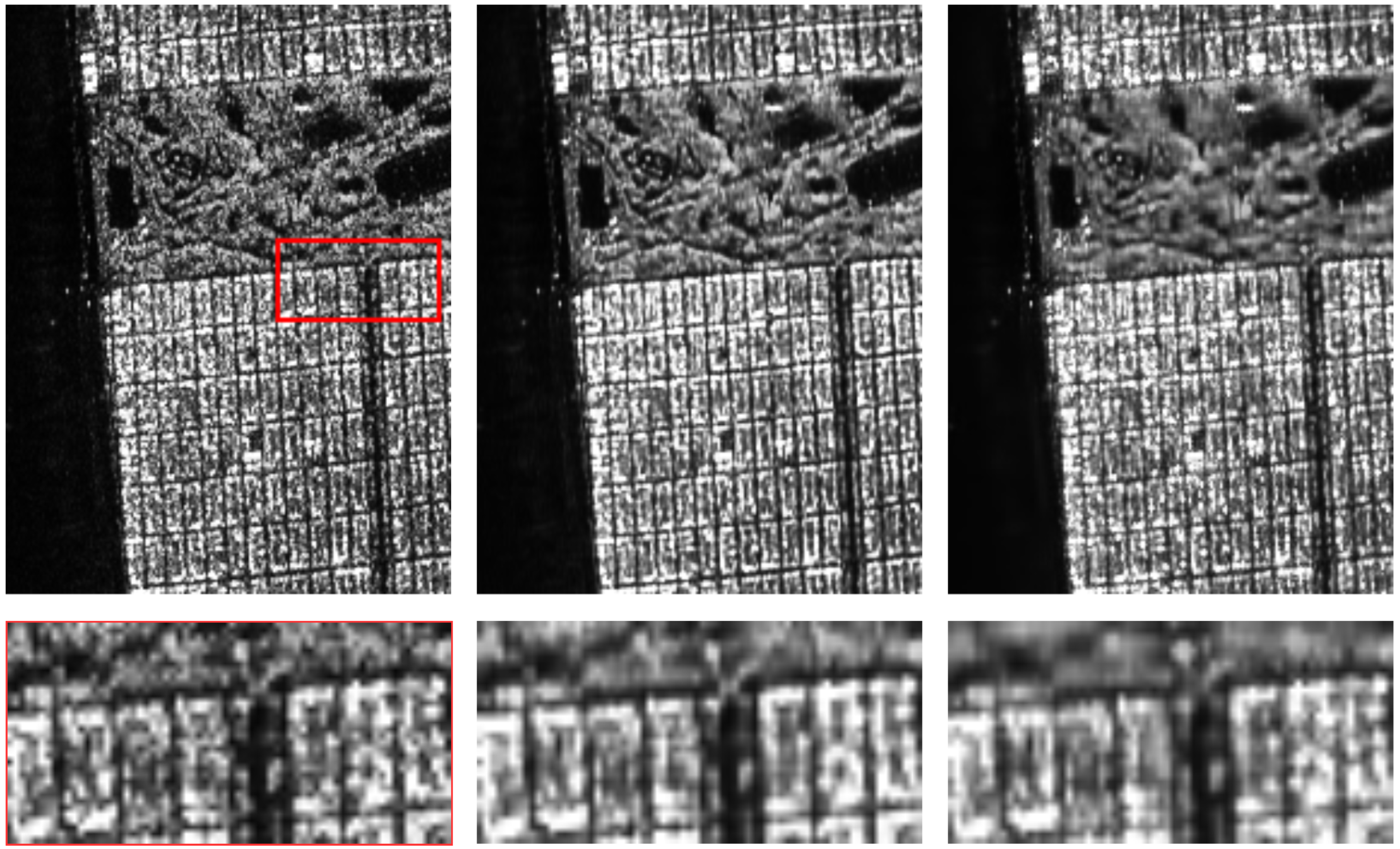
In order to eliminate the interference of the regularizer, and more accurately evaluate the eff of the loss function proposed in this article, we set the temperature parameter $\lambda$ to positive infinity in Speckle2Self. That is, the regularization term is discarded. In Figure 12, we show the despeckled results for the part of San Francisco with Speckle2Self using or not using a total variation (TV) regularizer. For Speckle2Self with TV, the temperature parameter $\lambda$ is set as $1e5$. It can be noticed that the TV regularizer smooths the image and suppresses noise more but at the expense of details. This is also consistent with the principle and consistent performance of the TV regularization term. The regularizer can be used as an adjuster to achieve a balance between smoothness and detail as needed.

5. Conclusions

In this article, we propose a novel self-supervised despeckling method for SAR images named Speckle2Self, which learns to restore images using noisy images only. A set of image masks is designed, and Speckle2Self outputs the despeckled result by predicting masked image pixel through the attention operation in the Transformer architecture. In addition, a loss function is also derived based on the statistics of SAR images, along with image downsampling for noise whitening. We conduct experiments on both synthetic and real image datasets, and experimental results demonstrate that the proposed Speckle2Self achieves comparable despeckling performance with supervised methods, suppressing noise while maintaining structural details (edges, lines). Ablation experiments verify the effectiveness of the proposed loss function and image-downsampling strategy. Compared with Speckle2Void, the proposed Speckle2Self not only has more advantages in the despeckling metrics but also does not rely on noise-level priors and has a wider application range. In the future, we plan to improve despeckling performance further and explore the potential of the proposed method in multi-channel SAR image despeckling.

References

1. Oliver, C.; Quegan, S. Understanding Synthetic Aperture Radar Images; SciTech Publishing: Raleigh, NC, USA, 2004. [Google Scholar]
2. Goodman, J.W. Some fundamental properties of speckle. J. Opt. Soc. Am. 1976, 66, 1145–1150. [Google Scholar] [CrossRef]
3. Touzi, R.; Lopes, A.; Bousquet, P. A statistical and geometrical edge detector for SAR images. IEEE Trans. Geosci. Remote Sens. 1988, 26, 764–773. [Google Scholar] [CrossRef]
4. Lee, J.S.; Grunes, M.R.; De Grandi, G. Polarimetric SAR speckle filtering and its implication for classification. IEEE Trans. Geosci. Remote Sens. 1999, 37, 2363–2373. [Google Scholar]
5. Lee, J.S. Digital image enhancement and noise filtering by use of local statistics. IEEE Trans. Pattern Anal. Mach. Intell. 1980, 30, 165–168. [Google Scholar] [CrossRef]
6. Lee, J.S. Speckle analysis and smoothing of synthetic aperture radar images. Comput. Graph. Image Process. 1981, 17, 24–32. [Google Scholar] [CrossRef]
7. Maji, S.K.; Thakur, R.K.; Yahia, H.M. SAR image denoising based on multifractal feature analysis and TV regularisation. IET Image Process. 2020, 14, 4158–4167. [Google Scholar] [CrossRef]
8. Frost, V.S.; Stiles, J.A.; Shanmugan, K.S.; Holtzman, J.C. A model for radar images and its application to adaptive digital filtering of multiplicative noise. IEEE Trans. Pattern Anal. Mach. Intell. 1982, 18, 157–166. [Google Scholar] [CrossRef]
9. Kuan, D.T.; Sawchuk, A.A.; Strand, T.C.; Chavel, P. Adaptive noise smoothing filter for images with signal-dependent noise. IEEE Trans. Pattern Anal. Mach. Intell. 1985, 37, 165–177. [Google Scholar] [CrossRef] [PubMed]
10. Lopes, A.; Touzi, R.; Nezry, E. Adaptive speckle filters and scene heterogeneity. IEEE Trans. Geosci. Remote Sens. 1990, 28, 992–1000. [Google Scholar] [CrossRef]
11. Kuan, D.; Sawchuk, A.; Strand, T.; Chavel, P. Adaptive restoration of images with speckle. IEEE Trans. Acoust. Speech Signal Process. 1987, 35, 373–383. [Google Scholar] [CrossRef]
12. Lopes, A.; Nezry, E.; Touzi, R.; Laur, H. Maximum a posteriori speckle filtering and first order texture models in SAR images. In Proceedings of the 10th Annual International Symposium on Geoscience and Remote Sensing, College Park, MD, USA, 20–24 May 1990; pp. 2409–2412. [Google Scholar]
13. Lopes, A.; Nezry, E.; Touzi, R.; Laur, H. Structure detection and statistical adaptive speckle filtering in SAR images. Int. J. Remote Sens. 1993, 14, 1735–1758. [Google Scholar] [CrossRef]
14. Lee, J.S.; Grunes, M.R.; Schuler, D.L.; Pottier, E.; Ferro-Famil, L. Scattering-model-based speckle filtering of polarimetric SAR data. IEEE Trans. Geosci. Remote Sens. 2005, 44, 176–187. [Google Scholar]
15. Argenti, F.; Lapini, A.; Bianchi, T.; Alparone, L. A tutorial on speckle reduction in synthetic aperture radar images. IEEE Geosci. Remote Sens. Mag. 2013, 1, 6–35. [Google Scholar] [CrossRef]
16. Bioucas-Dias, J.M.; Figueiredo, M.A. Multiplicative noise removal using variable splitting and constrained optimization. IEEE Trans. Image Process. 2010, 19, 1720–1730. [Google Scholar] [CrossRef] [PubMed]
17. Guo, H.; Odegard, J.E.; Lang, M.; Gopinath, R.A.; Selesnick, I.W.; Burrus, C.S. Wavelet based speckle reduction with application to SAR based ATD/R. In Proceedings of the 1st International Conference on Image Processing, Austin, TX, USA, 13–16 November 1994; Volume 1, pp. 75–79. [Google Scholar]
18. Solbo, S.; Eltoft, T. Homomorphic wavelet-based statistical despeckling of SAR images. IEEE Trans. Geosci. Remote Sens. 2004, 42, 711–721. [Google Scholar] [CrossRef]
19. Foucher, S. SAR image filtering via learned dictionaries and sparse representations. In Proceedings of the IGARSS 2008—2008 IEEE International Geoscience and Remote Sensing Symposium, Boston, MA, USA, 7–11 July 2008; Volume 1, pp. 1–229. [Google Scholar]
20. Jiang, J.; Jiang, L.; Sang, N. Non-local sparse models for SAR image despeckling. In Proceedings of the 2012 International Conference on Computer Vision in Remote Sensing, Xiamen, China, 16–18 December 2012; pp. 230–236. [Google Scholar]
21. Xu, B.; Cui, Y.; Li, Z.; Zuo, B.; Yang, J.; Song, J. Patch ordering-based SAR image despeckling via transform-domain filtering. IEEE J. Sel. Top. Appl. Earth Obs. Remote Sens. 2014, 8, 1682–1695. [Google Scholar] [CrossRef]
22. Xu, B.; Cui, Y.; Li, Z.; Yang, J. An iterative SAR image filtering method using nonlocal sparse model. IEEE Geosci. Remote Sens. Lett. 2015, 12, 1635–1639. [Google Scholar]
23. Buades, A.; Coll, B.; Morel, J.M. A review of image denoising algorithms, with a new one. Multiscale Model. Simul. 2005, 4, 490–530. [Google Scholar] [CrossRef]
24. Deledalle, C.A.; Denis, L.; Tupin, F. Iterative weighted maximum likelihood denoising with probabilistic patch-based weights. IEEE Trans. Image Process. 2009, 18, 2661–2672. [Google Scholar] [CrossRef] [PubMed]
25. Jojy, C.; Nair, M.S.; Subrahmanyam, G.R.S.; Riji, R. Discontinuity adaptive non-local means with importance sampling unscented Kalman filter for de-speckling SAR images. IEEE J. Sel. Top. Appl. Earth Obs. Remote Sens. 2012, 6, 1964–1970. [Google Scholar] [CrossRef]
26. Chen, J.; Chen, Y.; An, W.; Cui, Y.; Yang, J. Nonlocal filtering for polarimetric SAR data: A pretest approach. IEEE Trans. Geosci. Remote Sens. 2010, 49, 1744–1754. [Google Scholar] [CrossRef]
27. Vitale, S.; Cozzolino, D.; Scarpa, G.; Verdoliva, L.; Poggi, G. Guided patchwise nonlocal SAR despeckling. IEEE Trans. Geosci. Remote Sens. 2019, 57, 6484–6498. [Google Scholar] [CrossRef]
28. Dabov, K.; Foi, A.; Katkovnik, V.; Egiazarian, K. Image denoising by sparse 3-D transform-domain collaborative filtering. IEEE Trans. Image Process. 2007, 16, 2080–2095. [Google Scholar] [CrossRef]
29. Parrilli, S.; Poderico, M.; Angelino, C.V.; Verdoliva, L. A nonlocal SAR image denoising algorithm based on LLMMSE wavelet shrinkage. IEEE Trans. Geosci. Remote Sens. 2011, 50, 606–616. [Google Scholar] [CrossRef]
30. Chierchia, G.; Cozzolino, D.; Poggi, G.; Verdoliva, L. SAR image despeckling through convolutional neural networks. In Proceedings of the 2017 IEEE International Geoscience and Remote Sensing Symposium (IGARSS), Fort Worth, TX, USA, 23–28 July 2017; pp. 5438–5441. [Google Scholar]
31. Zhang, Q.; Yuan, Q.; Li, J.; Yang, Z.; Ma, X. Learning a dilated residual network for SAR image despeckling. Remote Sens. 2018, 10, 196. [Google Scholar] [CrossRef]
32. Gui, Y.; Xue, L.; Li, X. SAR image despeckling using a dilated densely connected network. Remote Sens. Lett. 2018, 9, 857–866. [Google Scholar] [CrossRef]
33. Pan, T.; Peng, D.; Yang, W.; Li, H.C. A filter for SAR image despeckling using pre-trained convolutional neural network model. Remote Sens. 2019, 11, 2379. [Google Scholar] [CrossRef]
34. Vitale, S.; Ferraioli, G.; Pascazio, V. Multi-objective cnn-based algorithm for sar despeckling. IEEE Trans. Geosci. Remote Sens. 2020, 59, 9336–9349. [Google Scholar] [CrossRef]
35. Deledalle, C.A.; Denis, L.; Tabti, S.; Tupin, F. MuLoG, or how to apply Gaussian denoisers to multi-channel SAR speckle reduction? IEEE Trans. Image Process. 2017, 26, 4389–4403. [Google Scholar] [CrossRef]
36. Wang, P.; Zhang, H.; Patel, V.M. SAR image despeckling using a convolutional neural network. IEEE Signal Process. Lett. 2017, 24, 1763–1767. [Google Scholar] [CrossRef]
37. Arbelaez, P.; Maire, M.; Fowlkes, C.; Malik, J. Contour detection and hierarchical image segmentation. IEEE Trans. Pattern Anal. Mach. Intell. 2010, 33, 898–916. [Google Scholar] [CrossRef]
38. Gu, F.; Zhang, H.; Wang, C.; Zhang, B. Residual encoder-decoder network introduced for multisource SAR image despeckling. In Proceedings of the 2017 SAR in Big Data Era: Models, Methods and Applications (BIGSARDATA), Beijing, China, 13–14 November 2017; pp. 1–5. [Google Scholar]
39. Liu, S.; Liu, T.; Gao, L.; Li, H.; Hu, Q.; Zhao, J.; Wang, C. Convolutional neural network and guided filtering for SAR image denoising. Remote Sens. 2019, 11, 702. [Google Scholar] [CrossRef]
40. Liu, R.; Li, Y.; Jiao, L. SAR image specle reduction based on a generative adversarial network. In Proceedings of the 2020 International Joint Conference on Neural Networks (IJCNN), Glasgow, UK, 19–24 July 2020; pp. 1–6. [Google Scholar]
41. Isola, P.; Zhu, J.Y.; Zhou, T.; Efros, A.A. Image-to-image translation with conditional adversarial networks. In Proceedings of the IEEE Conference on Computer Vision and Pattern Recognition, Honolulu, HI, USA, 21–26 July 2017; pp. 1125–1134. [Google Scholar]
42. Yang, Y.; Newsam, S. Bag-of-visual-words and spatial extensions for land-use classification. In Proceedings of the 18th SIGSPATIAL International Conference on Advances in Geographic Information Systems, San Jose, CA, USA, 2–5 November 2010; pp. 270–279. [Google Scholar]
43. Wang, P.; Zhang, H.; Patel, V.M. Generative adversarial network-based restoration of speckled SAR images. In Proceedings of the 2017 IEEE 7th international workshop on Computational Advances in Multi-Sensor Adaptive Processing (CAMSAP), Curacao, 10–13 December 2017; pp. 1–5. [Google Scholar]
44. Ferraioli, G.; Pascazio, V.; Vitale, S. A novel cost function for despeckling using convolutional neural networks. In Proceedings of the 2019 Joint Urban Remote Sensing Event (JURSE), Vannes, France, 22–24 May 2019; pp. 1–4. [Google Scholar]
45. Vitale, S.; Ferraioli, G.; Pascazio, V. A new ratio image based CNN algorithm for SAR despeckling. In Proceedings of the IGARSS 2019—2019 IEEE International Geoscience and Remote Sensing Symposium, Yokohama, Japan, 28 July–2 August 2019; pp. 9494–9497. [Google Scholar]
46. Yue, D.X.; Xu, F.; Jin, Y.Q. SAR despeckling neural network with logarithmic convolutional product model. Int. J. Remote Sens. 2018, 39, 7483–7505. [Google Scholar] [CrossRef]
47. Li, J.; Li, Y.; Xiao, Y.; Bai, Y. HDRANet: Hybrid dilated residual attention network for SAR image despeckling. Remote Sens. 2019, 11, 2921. [Google Scholar] [CrossRef]
48. Zhang, J.; Li, W.; Li, Y. SAR image despeckling using multiconnection network incorporating wavelet features. IEEE Geosci. Remote Sens. Lett. 2019, 17, 1363–1367. [Google Scholar] [CrossRef]
49. Cozzolino, D.; Verdoliva, L.; Scarpa, G.; Poggi, G. Nonlocal SAR image despeckling by convolutional neural networks. In Proceedings of the IGARSS 2019—2019 IEEE International Geoscience and Remote Sensing Symposium, Yokohama, Japan, 28 July–2 August 2019; pp. 5117–5120. [Google Scholar]
50. Cozzolino, D.; Verdoliva, L.; Scarpa, G.; Poggi, G. Nonlocal CNN SAR image despeckling. Remote Sens. 2020, 12, 1006. [Google Scholar] [CrossRef]
51. Tan, S.; Zhang, X.; Wang, H.; Yu, L.; Du, Y.; Yin, J.; Wu, B. A CNN-Based Self-Supervised Synthetic Aperture Radar Image Denoising Approach. IEEE Trans. Geosci. Remote Sens. 2021, 60, 1–15. [Google Scholar] [CrossRef]
52. Tang, X.; Zhang, L.; Ding, X. SAR image despeckling with a multilayer perceptron neural network. Int. J. Digit. Earth 2019, 12, 354–374. [Google Scholar] [CrossRef]
53. Fracastoro, G.; Magli, E.; Poggi, G.; Scarpa, G.; Valsesia, D.; Verdoliva, L. Deep learning methods for synthetic aperture radar image despeckling: An overview of trends and perspectives. IEEE Geosci. Remote Sens. Mag. 2021, 9, 29–51. [Google Scholar] [CrossRef]
54. Gomez, L.; Ospina, R.; Frery, A.C. Unassisted quantitative evaluation of despeckling filters. Remote Sens. 2017, 9, 389. [Google Scholar] [CrossRef]
55. Lehtinen, J.; Munkberg, J.; Hasselgren, J.; Laine, S.; Karras, T.; Aittala, M.; Aila, T. Noise2Noise: Learning image restoration without clean data. In Proceedings of the 35th International Conference on Machine Learning, Stockholm, Sweden, 10–15 July 2018; pp. 2965–2974. [Google Scholar]
56. Krull, A.; Buchholz, T.O.; Jug, F. Noise2void-learning denoising from single noisy images. In Proceedings of the IEEE/CVF Conference on Computer Vision and Pattern Recognition, Long Beach, CA, USA, 15–20 June 2019; pp. 2129–2137. [Google Scholar]
57. Batson, J.; Royer, L. Noise2self: Blind denoising by self-supervision. In Proceedings of the International Conference on Machine Learning, PMLR, Long Beach, CA, USA, 9–15 June 2019; pp. 524–533. [Google Scholar]
58. Quan, Y.; Chen, M.; Pang, T.; Ji, H. Self2self with dropout: Learning self-supervised denoising from single image. In Proceedings of the IEEE/CVF Conference on Computer Vision and Pattern Recognition, Seattle, WA, USA, 14–19 June 2020; pp. 1890–1898. [Google Scholar]
59. Laine, S.; Karras, T.; Lehtinen, J.; Aila, T. High-quality self-supervised deep image denoising. In Proceedings of the Advances in Neural Information Processing Systems 32, Vancouver, BC, Canada, 8–14 December 2019. [Google Scholar]
60. Yuan, Y.; Guan, J.; Feng, P.; Wu, Y. A practical solution for SAR despeckling with adversarial learning generated speckled-to-speckled images. IEEE Geosci. Remote Sens. Lett. 2020, 19, 1–5. [Google Scholar] [CrossRef]
61. Ravani, K.; Saboo, S.; Bhatt, J.S. A practical approach for SAR image despeckling using deep learning. In Proceedings of the IGARSS 2019—2019 IEEE International Geoscience and Remote Sensing Symposium, Yokohama, Japan, 28 July–2 August 2019; pp. 2957–2960. [Google Scholar]
62. Yuan, Y.; Guan, J.; Sun, J. Blind SAR image despeckling using self-supervised dense dilated convolutional neural network. arXiv 2019, arXiv:1908.01608. [Google Scholar] [CrossRef]
63. Zhang, G.; Li, Z.; Li, X.; Xu, Y. Learning synthetic aperture radar image despeckling without clean data. J. Appl. Remote Sens. 2020, 14, 026518. [Google Scholar] [CrossRef]
64. Joo, S.; Cha, S.; Moon, T. DoPAMINE: Double-sided masked CNN for pixel adaptive multiplicative noise despeckling. Proc. AAAI Conf. Artif. Intell. 2019, 33, 4031–4038. [Google Scholar] [CrossRef]
65. Deng, J.W.; Li, M.D.; Chen, S.W. Sublook2Sublook: A Self-Supervised Speckle Filtering Framework for Single SAR Images. IEEE Trans. Geosci. Remote Sens. 2024, 62, 5211613. [Google Scholar] [CrossRef]
66. Molini, A.B.; Valsesia, D.; Fracastoro, G.; Magli, E. Towards deep unsupervised SAR despeckling with blind-spot convolutional neural networks. In Proceedings of the IGARSS 2020—2020 IEEE International Geoscience and Remote Sensing Symposium, Waikoloa, HI, USA, 26 September–2 October 2020; pp. 2507–2510. [Google Scholar]
67. Dalsasso, E.; Denis, L.; Tupin, F. SAR2SAR: A semi-supervised despeckling algorithm for SAR images. IEEE J. Sel. Top. Appl. Earth Obs. Remote Sens. 2021, 14, 4321–4329. [Google Scholar] [CrossRef]
68. Mullissa, A.G.; Marcos, D.; Tuia, D.; Herold, M.; Reiche, J. DeSpeckNet: Generalizing deep learning-based SAR image despeckling. IEEE Trans. Geosci. Remote Sens. 2020, 60, 1–15. [Google Scholar] [CrossRef]
69. Molini, A.B.; Valsesia, D.; Fracastoro, G.; Magli, E. Speckle2Void: Deep self-supervised SAR despeckling with blind-spot convolutional neural networks. IEEE Trans. Geosci. Remote Sens. 2021, 60, 1–17. [Google Scholar] [CrossRef]
70. Ronneberger, O.; Fischer, P.; Brox, T. U-net: Convolutional networks for biomedical image segmentation. In Proceedings of the International Conference on Medical Computing and Computer-Assisted Intervention, Munich, Germany, 5–9 October 2015; pp. 234–241. [Google Scholar]
71. Vaswani, A.; Shazeer, N.; Parmar, N.; Uszkoreit, J.; Jones, L.; Gomez, A.N.; Kaiser, Ł.; Polosukhin, I. Attention is all you need. In Proceedings of the Advances in Neural Information Processing Systems 30, Long Beach, CA, USA, 4–9 December 2017. [Google Scholar]
72. He, K.; Zhang, X.; Ren, S.; Sun, J. Deep residual learning for image recognition. In Proceedings of the IEEE Conference on Computer Vision and Pattern Recognition, Las Vegas, NV, USA, 27–30 June 2016; pp. 770–778. [Google Scholar]
73. Ba, J.L.; Kiros, J.R.; Hinton, G.E. Layer normalization. arXiv 2016, arXiv:1607.06450. [Google Scholar] [CrossRef]
74. Lin, T.; Wang, Y.; Liu, X.; Qiu, X. A survey of transformers. arXiv 2021, arXiv:2106.04554. [Google Scholar] [CrossRef]
75. Lapini, A.; Bianchi, T.; Argenti, F.; Alparone, L. Blind speckle decorrelation for SAR image despeckling. IEEE Trans. Geosci. Remote Sens. 2013, 52, 1044–1058. [Google Scholar] [CrossRef]
76. Hamza, A.B.; Krim, H. A variational approach to maximum a posteriori estimation for image denoising. In Proceedings of the International Workshop on Energy Minimization Methods in Computer Vision and Pattern Recognition, Sophia Antipolis, France, 3–5 September 2001; pp. 19–34. [Google Scholar]
77. Dosovitskiy, A.; Beyer, L.; Kolesnikov, A.; Weissenborn, D.; Zhai, X.; Unterthiner, T.; Dehghani, M.; Minderer, M.; Heigold, G.; Gelly, S.; et al. An image is worth 16x16 words: Transformers for image recognition at scale. arXiv 2020, arXiv:2010.11929. [Google Scholar]
78. Cui, Y.; Zhou, G.; Yang, J.; Yamaguchi, Y. Unsupervised estimation of the equivalent number of looks in SAR images. IEEE Geosci. Remote Sens. Lett. 2011, 8, 710–714. [Google Scholar] [CrossRef]
79. He, K.; Zhang, X.; Ren, S.; Sun, J. Delving deep into rectifiers: Surpassing human-level performance on imagenet classification. In Proceedings of the IEEE International Conference on Computer Vision, Santiago, Chile, 7–13 December 2015; pp. 1026–1034. [Google Scholar]
80. Anfinsen, S.N.; Doulgeris, A.P.; Eltoft, T. Estimation of the equivalent number of looks in polarimetric synthetic aperture radar imagery. IEEE Trans. Geosci. Remote Sens. 2009, 47, 3795–3809. [Google Scholar] [CrossRef]
81. Lin, H.; Jin, K.; Yin, J.; Yang, J.; Zhang, T.; Xu, F.; Jin, Y.Q. Residual In Residual Scaling Networks for Polarimetric SAR Image Despeckling. IEEE Trans. Geosci. Remote Sens. 2023, 61, 5207717. [Google Scholar] [CrossRef]
Figure 1. Architecture of the proposed Speckle2Self consists of four modules: image masking, contextual information pooling, masked pixel prediction, and self-supervision. Given a log-transformed SAR image, we first bind the image pixels at selected positions through element-wise multiplication of the SAR image and a designed mask. Then, the masked image is split into patches, and fed into the Transformer encoder for image information pooling. On the other hand, we use another complementary mask as queries, whose non-zero elements indicate the pixels to be despeckled. Similarly, the queries are split into patches, positional embedded, cross-attentioned, and put into the Transformer decoder to predict the despeckled values of the selected target pixels. Finally, the masked pixels, serving as groundtruth, are utilized to cooperate with the despeckled image pixels for self-supervised training, under the guidance of the proposed loss function.
Remotesensing 17 03840 g001
Figure 2. Plots of (a) 10 log 10 [ | R v v ( m , 0 ) / R v v ( 0 , 0 ) | ] and (b) 10 log 10 [ | R v v ( 0 , n ) / R v v ( 0 , 0 ) | ] .
Remotesensing 17 03840 g002
Figure 3. Visualization of the designed mask set b 3 , 3 j j = 0 j = 8 for an image with size 9 × 9 .
Remotesensing 17 03840 g003
Figure 4. Comparison of despeckled results for the Monarch (top two rows) and Pepper (bottom two rows). The ENL of the noisy images for the Monarch and Pepper are 1 and 4, respectively. From left to right: Noisy, PPB, SAR-BM3D, ID-CNN, Speckle2void, Speckle2Self.
Remotesensing 17 03840 g004
Figure 5. Comparison of despeckling results on synthetic SAR images (top row) and the corresponding Canny edge-detection outputs (bottom row). The ENL of the noisy input images is 2. From left to right: Noisy, PPB, SAR-BM3D, ID-CNN, Speckle2Void, and Speckle2Self.
Remotesensing 17 03840 g005
Figure 6. Comparison of the despeckled results for the Image-5 of the test images in [69] ( L = 0.87 ). The homogeneous area marked by the green box is used for ENL estimation. Top-left to bottom-right: Noisy, PPB, SAR-BM3D, ID-CNN, Speckle2void, Speckle2Self.
Remotesensing 17 03840 g006
Figure 7. Comparison of the despeckled results for Flevoland ( L = 2.99 ). The homogeneous area marked by the green box is used for ENL estimation. Top-left to bottom-right: Noisy, PPB, SAR-BM3D, ID-CNN, Speckle2void, Speckle2Self.
Remotesensing 17 03840 g007
Figure 8. Ratio images for Dalian ( L = 1.02 ). Top-left to bottom-right: Noisy, PPB, SAR-BM3D, ID-CNN, Speckle2void, Speckle2Self. PPB exhibits prominent dark-spot artifacts, while ID-CNN reveals distinct linear edges, particularly in urban regions. SAR-BM3D and Speckle2Void reduce structural artifacts but still display some heterogeneous patterns. The proposed Speckle2Self produces the most homogeneous ratio image, indicating effective speckle suppression with minimal residual artifacts.
Remotesensing 17 03840 g008
Figure 9. Comparison between Speckle2Void and the proposed Speckle2Self for Dalian ( L = 1.02 ). The homogeneous area marked by the green box is used for ENL estimation.The despeckling performances of Speckle2Void is highly related to the input of ENL. Inappropriate ENL settings would severely degrade the despeckling performances of Speckle2Void.
Remotesensing 17 03840 g009
Figure 10. Comparison of the despeckled results using different loss functions for the part of Dalian ( L = 1.02 ). From left to right: Noisy, Speckle2Self using l 2 loss function, Speckle2Self using l 1 loss function, Speckle2Self using the proposed loss function.
Remotesensing 17 03840 g010
Figure 11. Comparison of the despeckled results with/without image downsampling for the part of Singapore ( L = 2.48 ). From left to right: Noisy, Speckle2Self without image downsampling, Speckle2Self with image downsampling.
Remotesensing 17 03840 g011
Figure 12. Comparison of the despeckled results with/without TV for the part of San Francisco ( L = 2.73 ). From left to right: Noisy, Speckle2Self without TV, Speckle2Self with TV.
Remotesensing 17 03840 g012