Highlights
What are the main findings?
- A novel multi-scale validation (field, UAV, Landsat) demonstrates that MODIS CI products show good agreement with reference data (R = 0.75, RMSE = 0.05) in a temperate forest. Direct “point-to-pixel” comparisons are highly susceptible to subpixel heterogeneity.
- Semivariogram analysis of the high-resolution CI map reveals that a ~209 m observational footprint is required for a spatially representative sample, critically informing future validation design for coarse-resolution products.
What is the implication of the main finding?
- The study provides a robust framework that enables diagnosis of error sources, distinguishing between uncertainties from satellite retrieval (e.g., land cover misclassification causing errors up to 0.33) and those introduced by the validation process itself (e.g., upscaling method choice).
- Findings confirm the operational utility of MODIS CI while underscoring the necessity for international cooperative campaigns to obtain representative field data and further research on scaling methods for extensive global validation.
Abstract
The clumping index (CI) describes the level of foliage grouping relative to the random distribution within the canopy. It plays a vital role in the derivation of other important parameters (e.g., the leaf area index, (LAI)) that are usually employed in hydrological, ecological and climatological modeling. In recent years, several satellite-based CI products have been developed using multi-angle reflectance data. However, these products have been validated through the use of a “point-to-point” comparison, which rarely involves a quantitative analysis of spatial representativeness for field-measured CIs in most cases. In this study, we developed a methodological framework to validate the MODIS CI at three different data scales on the basis of intense field measurements, high-resolution unmanned aerial vehicle (UAV) observations and Landsat 8 data. This framework was used to understand the impacts of the scale issue and subpixel variance of the CI in the validation of the MODIS CI for a case study of 12 gridded 500 m pixels in Saihanba National Forest Park, Hebei, China. The results revealed that the MODIS CIs in the study area were in good agreement with the upscaled field CIs (R = 0.75, RMSE = 0.05, bias = 0.02) and UAV CIs. Through a comparison of the observed CIs along the 30 m transects with the 500 m MODIS CIs, we gained insight into the uncertainty caused by the direct “point-to-pixel” evaluation method, which ranged from −0.21~+0.27 for the 10th and 90th percentiles of the observed-MODIS CI error distribution for the twelve pixels. Moreover, semivariogram analysis revealed that the representativeness assessments based on high-resolution albedo and CI maps could reflect the spatial heterogeneity within pixels, whereas the CI map provided more information on the variation in vegetation structures. The average observational footprint needed for a spatially representative sample is approximately 209 m according to an analysis of the high-resolution CI map. The uncertainty of mismatched MODIS land cover types can lead to a deviation of 0.33 in CI estimates, and compared with the CLX method, the scaled-up CI method based on simple arithmetic averages tends to overestimate CIs. In summary, various validation efforts in this case study reveal that the accuracy of the MODIS CIs is generally reliable and in good agreement with that of the upscaled field CIs and UAV CIs; however, with the development of surface process modeling and remote sensing technology, substantial measurements of field CIs in conjunction with high-resolution remotely sensed CI maps derived from single-angle advanced methods are urgently needed for further validation and potential applications. Certainly, such a validation effort will help to improve the understanding of MODIS CI products, which, in turn, will further support the methods and applications of global geospatial information.
1. Introduction
The clumping index (CI) is an important structural parameter of vegetation canopies. It characterizes the grouping of foliage in the canopy relative to its random distribution. Foliage CI plays a vital role in accurate estimation of the leaf area index (LAI) [1], the fraction absorbed photosynthetically active radiation (FPAR) [2,3] and the canopy-level gross primary production (GPP) [4,5], which in turn are very important for hydrological, ecological and climatological modeling [6,7,8]. Previous studies have shown that CI is highly spatially variable, even within the same land cover type [9,10]; therefore, providing a credible spatial distribution map of the CI using remote sensing data is highly desirable [8,11]. Chen et al. [12,13] first proposed that an angular index named the normalized difference between hotspot and darkspot (NDHD) has the potential to estimate the CI. This was accomplished by developing the linear NDHD−CI relationship that was in turn generated through a so-called 4-scale geometric-optical (GO) model simulation [13]. Subsequently, several global maps of CI have been successfully derived from multi-angular satellite data on the basis of such a relationship, e.g., the Polarization and Directionality of Earth Reflectances (POLDER) [12,14,15,16], Moderate Resolution Imaging Spectroradiometer (MODIS) [9,17,18,19,20,21,22] and the Multi-angle Imaging Spectroradiometer (MISR) [23] data.
As one of the important parameters determining the interaction between plants and incident radiation, reasonable satellite-based CIs with comprehensive and reliable data validation are needed in studies of biophysical parameter inversions, atmosphere-ecosystem interactions, and global change [4,24,25,26]. For example, a previous study reported that the LAIs measured in conifer stands under the assumption of a random spatial distribution of foliage in plant canopies (i.e., CI = 1.0) were typically 50–70% direct estimates of the true LAI [24]. A typical conifer forest with an LAI of 4 and a CI of 0.5, assuming that the albedos above and below the canopy were 5% and 6%, respectively, would have a relative error of 23.5% in FPAR estimation without considering the CI [8]. Furthermore, ignoring the CI would cause an approximately 12% overestimation of the global GPP, even if accurate LAI data were used [4]. In short, to better serve the needs of the relevant studies mentioned above, accurate estimation and reliable validation of the CI are desperately needed.
Previously, CI validation methods were mostly based on direct “point-to-pixel” comparisons using site observations, somewhat depending on different CI measurement methods [16,17,19], most likely because appropriate high-resolution CI maps are rarely available and intense field CI measurements within validation sites are arduous and time-consuming. In an early effort, Leblanc et al. [15] validated the POLDER CI of Canada using the range of field-measured CIs of nine vegetation cover types observed by Tracing Radiation and Architecture of Canopies (TRAC) and hemispherical photography (HP). Piesk et al. [16] validated the ~6 km global POLDER CI by direct comparison with 32 field CIs measured by TRAC and reported that while the evaluation was inevitably limited because of the lack of high-resolution imagery, CI observations with TRAC were likely an optimum choice for validation, as it could collect data along transects of tens or hundreds of meters. Recently, Zhu et al. [21] validated 500 m MODIS CI in China directly using field measurements of TRAC and reported that spatial scale effects might induce disagreement between measured and retrieved CI. He et al. [17] and Piesk et al. [23] validated 500 m MODIS CI and 275 m MISR CI by directly comparing them with field measurements and reducing the effect of scale difference by using pure pixels and spatially homogeneous sites, which are determined on the basis of field observations and Google Maps. Most recently, Jiao et al. [19] validated the 500 m MODIS CI by first analyzing the spatial representativeness of the 500 m pixels using Landsat reflectance, on the basis of the evaluation method developed by Román et al. [27], and then selected 48 field measurements with spatial representativeness to validate the derived MODIS CIs. In general, these studies have revealed the potential uncertainties caused by the scale effect of “point-to-pixel” comparisons in the process of CI validation. However, owing to the absence of appropriate high-resolution CI data and intense field measurements, the main strategies that these studies adopted to reduce potential uncertainty in the validation of the retrieved CIs at the pixel scale were to choose so-called pure pixels within homogeneous sites determined by a high-resolution reflectance map (instead of a high-resolution CI map). Therefore, analyses of CI variations within pixels have rarely been performed in existing validation efforts.
Despite such a challenge in the validation of CI products, a validation method for other moderate-resolution satellite products (e.g., LAI products, albedo products) has been developed for a relatively reasonable intercomparison framework [27,28,29,30,31,32,33,34,35], which can provide a valuable reference for the assessment of CI products. For example, Fernandes et al. [28] presented the best-practice protocol for LAI validation and reported that the direct validation of moderate-resolution LAI corresponds to the comparison between the temporally and spatially concurrent satellite-derived LAI products and upscale in situ reference LAI estimates. Fang et al. [32] summarized the validation schemes of LAI products and reported that the upscaling process of field LAIs is mainly based on the establishment of a transfer function between the measurements and a high-resolution reference or vegetation index derived from satellite or airborne data. Similarly, owing to the considerable scale difference between satellite-based CI and in situ observations, the validation of satellite-based CI products needs to consider such a method in which the field CI measurements can be scaled up to a comparable pixel scale so that further analysis can be implemented within these validation pixels. Indeed, efforts have already been made to obtain upscale in situ CI estimates in previous studies, e.g., the VALERI project (http://w3.avignon.inra.fr/valeri/, accessed on 24 August 2025), which is dedicated to the validation of biophysical products derived from moderate-resolution satellite sensors. Sites from this project are approximately 3 × 3 km2 in size and flat and relatively homogeneous, and corresponding 30 m CI maps were generated by using the 30 m effective LAI and true LAI maps. The latter two maps are generated by establishing transfer functions to relate the ground measurements of the biophysical variables to those of the high-resolution reflectance or vegetation indices. This dataset was used by Wei and Fang [20] to evaluate the MODIS and MISR CIs at the landscape scale (500 m or 250 m) and site scale (3 km). Two upscaling methods of ground CI, i.e., the arithmetic average (CIAVG) and gap fraction (CIGap) methods, were discussed, and CIGap was ultimately recommended to obtain the upscale ground CI estimates. While the methods mentioned above have been used to improve the understanding of the validation of satellite CI products to some extent, analyses of the variation in CI within moderate-resolution pixels, which is critical for exploring scale issues, have not been comprehensively performed.
A potential way to directly acquire high-resolution CI data that serve as a bridge for “point-to-pixel” comparison is to obtain airborne high-resolution multi-angle reflectance observations, which can obtain high-resolution CI maps similarly to the CI−NDHD relationship [36,37]; however, such data are mainly limited mainly because of the high cost and operational requirements. In recent years, with the development of unmanned aerial vehicle (UAV) technology, obtaining high-resolution multi-angle surface reflectance data for in situ measurements has become relatively feasible. Considering the advantages of the flexibility and high resolution of UAV observations, involving these promising data in the validation and scale effect analysis of satellite-based CIs is meaningful. In addition, various techniques for field CI measurements such as TRAC, digital hemispheric photography (DHP), and optical plant canopy analyzer (PCA), have been developed and frequently used to measure in situ CI. Considering that the scopes of single observations of DHP and PCA are determined mainly by the field of view of the lens of the instrument and are usually smaller than those of TRAC, which in turn relies on the length of the measured transect, CI measurements for a forest validation site using TRAC are more likely to be spatially representative and are thus recommended [16].
In this study, we designed a methodological framework to implement a comprehensive validation for MODIS CI products [19] by using multi-source data collected in Saihanba National Forest Park. Current validation approaches for satellite-derived CI products often rely on limited field measurements, leading to uncertainties in “point-to-pixel” comparisons and insufficient assessment of scale effects and spatial representativeness. To address these issues, our framework integrates field measurements, UAV multi-angle observations, and Landsat 8 reflectance data, enabling cross-scale validation from fine to coarse resolutions. The 500 m MODIS CIs were validated and analyzed at three different data scales, i.e., the 1st scale of field measurements obtained by TRAC with 30 m transects; the 2nd scale of 30 m resolution CI maps derived by using TRAC CIs and Landsat reflectance data; and the 3rd scale of CIs with an equivalent 500 m transect inferred by aggregating gap observations with corresponding tracks. In addition, the UAV multi-angle observations were used to retrieve a series of CIs of 10~100 m resolution on the basis of the CI–NDHD relationships, which were used to explore the scale effect of the CI retrievals by comparison with the corresponding 500 m MODIS CI. This multi-level approach provides a more robust basis for evaluating the accuracy and subpixel variability of MODIS CI. Moreover, the framework systematically analyzes the impact of land cover misclassification on CI retrieval. Our work offers a novel and structured methodology for improving the validation of CI products, with enhanced insights into scale-related uncertainties and spatial consistency.
2. Data
2.1. Field Data
2.1.1. Study Area
The study area is located in the Matikeng forest district of Saihanba National Forest Park (42°24′–42°25′N, 117°19′–117°21′E), northern Hebei Province, China (Figure 1), and contains twelve 500 m gridded MODIS pixels, which are numbered from P0101 to P0304, where “P” is the initial “pixel”, and the first two numbers indicate the rows, while the last two numbers indicate the columns. The field experiment in this study is part of the remote sensing field campaign of the carbon cycle, hydrologic cycle and energy balance, organized by the State Key Laboratory of Remote Sensing Science [38,39]. The Saihanba National Forest Park has the largest plantation in China and is an important nature reserve for endangered animals and plants inhabiting the forest-stepped ecotone. This area has a cold temperate monsoon climate, with long, cold winters and short, cool summers. The annual average temperature is approximately −1.4 °C and the mean annual precipitation is approximately 452 mm, which is concentrated mainly from June to August [40]. The main tree species in the study area are larch (Larix principis-rupprechtii), pine (Pinus sylvestris var. mongolica) and birch (Betula platyphylla), of which the coniferous forests are planted, while the birch grows naturally. The man-made forest was raised in 1964 and retained approximately 375 trees/ha after tending and thinning. The average height of the trees is approximately 20 m, while the mean breast diameter is approximately 25 cm. The study region has an average altitude of 1604 m, which is higher in the northeast and lower in the southwest. Most of the study area is flat, with slopes < 5°, whereas the northeastern and east-central regions are relatively rugged, with slopes reaching ~25°.
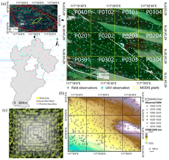
Figure 1.
Location of the study area and distribution of field observations in the Luan River Basin of Hebei Province, China. (a) The location of the study area and the distribution of observation sites. Specifically, the true color remote sensing image is processed using 10 m Sentinel-2B Level 1C data on 5 September, 2018 (50TNM and 50TNN; https://scihub.copernicus.eu/, accessed on 20 March 2023); the twelve 500 m gridded MODIS pixels are labeled “P0X0X”, as shown in the upper-right corner; the arrows indicate the location of the study area within the Xiaoluanhe River Basin, Hebei Province. (b) Digital Elevation Model (DEM) data of the study area, which were processed using 30 m Shuttle Radar Topography Mission (SRTM) data (N42E117; http://dwtkns.com/srtm30m/, accessed on 24 August 2025). (c) Schematic of the upscaling of multi-angle UAV observations to multi-resolution ranging from 10 m to 100 m at 10 m intervals, corresponding to the UAV observation site (★) in grid P0202 in the upper-right subfigure of (a).
2.1.2. TRAC Measurements
The TRAC is an optical instrument that acquires the gap size distribution through recording the photosynthetic photon flux density at a high frequency (32 Hz) [41]. The TRAC operator is required to walk under the canopy with an orientation perpendicular to the sunlight at a steady pace (approximately 0.3 m per second is recommended). On sloping grounds, the direction of the measurement transects was parallel to the slope to reduce the effect of the terrain. Moreover, the recommended solar zenith angle (SZA) of observation is 30–60° to reduce the uncertainties caused by weak radiation, and by approximation of the foliage projection function G(θ), the G-function is always close to 0.5 at a range from 50° to 60° and is essentially invariant at 0.5 over different leaf angle distributions at an SZA = 57.5° [42]. To satisfy these conditions as much as possible, field measurements were conducted from 8:00 a.m. to 6:00 p.m.
As shown in Figure 1, a total of 321 observations were collected in the study area during two time periods, 12–15 June and 24–31 August, and each observation was acquired by TRAC with a 30 m transect with records for locations and land cover types. Given that the grass (~19%) in the study area is too short for TRAC measurement, only forests (~78%) were measured. For each 500 m gridded MODIS pixel, approximately 27 samples were observed on average, and the exact number of samples depended mainly on the proportion of forestland area, the heterogeneity of forestland and the complexity of the terrain (reachability) within the pixel. More details about the field observations can be found in the Appendix A.
2.2. UAV Data
The UAV data used in this study were acquired on 21 August 2019 over a sample plot of larch (Figure 1) by the International Institute for Earth System Science (ESSI) of Nanjing University [43]. The multi-angle reflectance data were acquired using the GaiaSky-mini2-VN hyperspectral imager (Dualix instruments Ltd., Chengdu, Sichuan, China) aboard the DJI Matrice 600 Pro drone. The hyperspectral imager can collect the surface reflectance in the spectral region from 400 to 1000 nm with spectral resolution of 3.5 nm. The data were collected at an altitude of 200 m above ground level, and the swath width of the nadir was approximately 100 m. Observations in the view zenith angle (VZA) every 10° from 60° in the backward scattering direction (VZA = −60°) to 60° in the forward scattering direction, and in the direction of the hotspot (VZA = −30.7°) and darkspot (VZA = 32°) were captured approximately along the solar principal plane with an SZA = 32°. During the drone flight period, the ASD FieldSpec 3 spectroradiometer was used to measure the field spectra of a gray reference panel and typical tree species (i.e., larch) to calibrate the drone-based multi-angle reflectance data. The data were processed by the ESSI of Nanjing University as follows: (1) the calibration files of the hyperspectral imager were used to perform the lens correction; (2) the multi-angle reflectance data were calculated using the field spectra of the gray reference panel; (3) the Savitzky-Golay filter was used to smooth the measured multi-angle hyperspectral reflectance data; and (4) the arithmetic average method was used to scale up the hyperspectral reflectance image to a range of spatial resolution maps from 10 m to 100 m with 10 m intervals (Figure 1). The multi-angle reflectance data of different spatial resolutions of the red band (645 nm) were used to retrieve CIs in this study, to be spectrally consistent with the MODIS CI product in the red band (620–670 nm).
To reconstruct the reflectance in the exact hotspot direction and reduce the uncertainty caused by the potential unstable drone flight attitude, which is susceptible to weather conditions and operations, a hotspot-corrected BRDF model [44] was used to retrieve the bidirectional reflectance factor (BRF) of the hotspot and darkspot. First, the BRDF model was used to fit the reflectance data on the basis of a set of multi-angle reflectance observations. Afterward, the best fitting values of the two hotspot parameters were derived to reconstruct the reflectance in the exact hotspot direction. Once the minimum darkspot reflectance of the observations in the forward scattering direction is determined through the BRDF models, a similar CI–NDHD relationship can be driven to acquire the UAV CIs as the final step.
2.3. MODIS Data
As the MODIS CI products have been released up to 2021, the daily and monthly MODIS CI data consistent with the field observations were calculated by using the same algorithm [19] based on MODIS C006 500 m daily BRDF model parameter product (MCD43A1), daily BRDF quality product (MCD43A2) and yearly land cover type product (MCD12Q1). The daily BRDF model parameter product and its corresponding quality product were generated by weighting high-quality surface reflectance observations acquired from the Terra and Aqua sensors over a 16-day period. The three model parameters (isotropic, volumetric and geometric) from MCD43A1, and the band-dependent BRDF quality flags of the red band from MCD43A2, were used to derive MODIS CI. Furthermore, the International Geosphere-Biosphere Programme (IGBP) land cover data in MCD12Q1 was used as a land cover type flag to determine the canopy crown shape in the CI retrieval algorithm [12,19].
2.4. FROM-GLC Data
In the study area, 30 m LC data are needed to obtain a 30 m CI map for further validation and analysis. To examine subpixel variance within the MODIS IGBP classes, in conjunction with field-observed land cover types, the 30 m LC map can provide finer information to analyze the uncertainties caused by some potentially misclassified IGBP pixels in CI retrievals. The 30 m Finer Resolution Observation and Monitoring Global Land Cover (FROM-GLC) version 2 (2015_v1) data (Figure 2b) were downloaded and compared with field observations. This data was obtained from the Star Cloud Data Service Platform (https://data-starcloud.pcl.ac.cn/, accessed on 9 August 2025) which was derived based on a Random Forest (RF) algorithm using Landsat data [45,46]. Unfortunately, these LC data did not exactly match the field-observed types; thus, the 30 m LC map had to be reproduced through the random forest method by using field observations and Landsat 8 multi-spectral reflectance data in this study area.
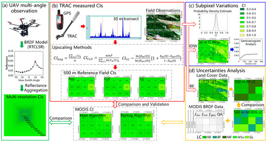
Figure 2.
Validation framework of this case study. The framework includes four major modules, i.e., (a) UAV multi-angle observations, (b) TRAC measured CIs, (c) Subpixel variations, and (d) Uncertainty analysis. The arrows depict the flow of data within the validation framework.
2.5. Landsat 8 OLI Data
The 30 m Landsat 8 Operational Land Imager (OLI) surface reflectance data captured on 15 September 2018 (Figure 3a) were used in this study. The surface reflectance data, as well as their derived spectral indices, were generated by the Landsat 8 Surface Reflectance Code (LaSRC) algorithm and downloaded from the U.S. Geological Survey (USGS) Earth Resources Observation and Science (EROS) Center Science Processing Architecture (ESPA) on-demand interface (https://espa.cr.usgs.gov/, accessed on 9 August 2025) [47]. On the one hand, these data were used to reproduce the 30 m LC map of the study area as mentioned above; on the other hand, they were used to obtain the 30 m CI map of the study area by establishing transfer functions between reflectances and field measured parameters, which were already used in previous studies [20,29,32,48,49,50]. To obtain 30 m CI data by the transfer function method, the 30 m true LAI and effective LAI map were first acquired through developed transform functions between surface reflectance and these two biophysical variables, respectively, on the basis of the least squares principle; then, the CI map was obtained by dividing the effective LAI by the true LAI [12,20]. Because the 30 m CI map calculated by the transform function method was weakly correlated with the field observations, especially for coniferous forest, which accounts for a high percentage of the area in the study region, the spatial interpolation method was ultimately used to obtain a 30 m CI map for further subpixel analysis, given the dense field observations in this specific case study.
3. Methods
3.1. CI Retrieval Algorithm
The retrieval algorithm, which was used to produce the global MODIS CI product [19], was used to calculate the UAV CI in accordance with field observations. This algorithm framework includes the main algorithm and backup algorithm, and constrains the retrieved CIs to the closed interval [0.33, 1.0] through analysis of the theory of BRDF variability for vegetation canopies in the principal plane, which is based on the relationship between NDHD and CI. To retrieve the CI from multi-angle reflectance data, first, the hotspot-adjusted BRDF model with two optimized hotspot parameters was used to fit the BRFs; then, the reflectances in the direction of the hotspot (45° in backward scattering) and darkspot (45° in forward scattering) were reconstructed; finally, the NDHD and CI were calculated in conjunction with the LC data on the basis of the linear relationships established by the 4-Scale model [12,13,36]. In particular, if the derived CI is outside the closed interval [0.33, 1.0], a backup algorithm based on the anisotropic flat index (AFX) [51,52] is adopted to process the so-called outlier.
The original kernel-driven BRDF models were first proposed by Roujean et al. [53] and are generally presented as an empirical, linear combination of three typical scattering components, i.e., isotropic scattering, volumetric scattering, and geometric-optical (GO) scattering [53,54,55]:
where R(θv,θs,Δφ,λ) refers to the BRFs in the waveband λ; Kvol(θv, θs, Δφ) and Kgeo(θv, θs, Δφ) are the kernels of volumetric and GO scattering components, which are designed as trigonometric functions of the view zenith θv, illumination zenith θs and relative azimuth Δφ; fiso(λ), fvol(λ) and fgeo(λ) are spectrally dependent weight coefficients of isotropic, volumetric and GO scattering components, respectively.
Recently, a method has been developed to improve the ability of the hotspot effect of RossThick-LiSparseReciprocal (RTLSR) model, which has been used as the operational MODIS BRDF algorithm [44]. As the RTLSR model was reported to often underestimate the hotspot effect [44,56,57], i.e., hotspot height and hotspot width, an exponential approximation of the hotspot kernel was improved and used to correct the hotspot effect of the volumetric scattering component for the RTLSR model. This hotspot corrected model (i.e., RTCLSR) with two prior hotspot parameter values (i.e., 0.7 and 3.2) was used to reconstruct the BRFs of hotspot (ρHS) and darkspot (ρDS). Then the NDHD can be obtained by:
According to the linear CI–NDHD equations in the red band [12,13], which are derived by the 4-scale model simulation, the CI can ultimately be obtained in association with a priori classification information. For coniferous forests:
For the other vegetation classes:
For the backup algorithm, the AFX was used to find the most similar BRDF archetype of the same land cover type and provide the most likely estimation of the CI for pixels outside the closed interval [0.33, 1.0] in terms of the main algorithm. AFX is calculated using the BRDF model parameters:
where WSA(λ) is the white sky albedo; Hvol and Hgeo are bi-hemispherical integral values of volumetric and GO scattering kernels. Then, corresponding CIs can be found through a CI–AFX look-up-table (LUT) established by using the CI–NDHD relationship based on the average BRDF shape (i.e., BRDF archetype) determined by AFX [19].
As the BRDF and LC data play indispensable roles in the CI retrieval algorithm, the influence of the uncertainties caused by the accuracy of the BRDF parameter data and the LC data on the CI retrievals was analyzed in this case study. Specifically, fully considering the BRDF quality information when applying the MODIS BRDF/albedo data was necessary; otherwise users were susceptible to drawing inaccurate conclusions [30,31,58]. Therefore, the influence of the quality of the BRDF parameters on the CI retrievals was further analyzed in this case study. In addition, the LC classification map must be used as important ancillary information to constrain the application of canopy structure-specific CI–NDHD equations in the algorithm, particularly between the needleleaf and broadleaf species, because the needleleaf forests present an additional hierarchical clumping structure (i.e., needle-to-shoot area ratio). Consequently, the uncertainties in the LC classification map, especially those caused by classification confusion between coniferous forests and other vegetation types, strongly influence the accuracy of CI retrieval in theory. Fortunately, the misclassified coniferous type was not difficult to identify in the field campaign in this case study and was thus further analyzed in a practical way, e.g., by generating a high-accuracy land cover map through the random forest (RF) method (Section 3.2.1) based on these dense field investigation samples as training data. Such a classification map tends to have a higher classification accuracy in the case study, which is, in turn, readily comparable to the use of the current classification product map for further analysis of the uncertainty in class-based CI retrieval.
Notably, considering the potentially seasonal variation in foliage clumping features for vegetation phenology [11,59,60], the field campaign was designed to represent such a seasonal difference in terms of two periods, i.e., 12–15 June and 24–31 August 2018. However, after a statistical hypothesis testing, no significant difference was detected in the measured CIs between these two periods. Therefore, all the field CIs in each 500 m gridded MODIS pixel were equally used in the scale-up process, as shown in Section 3.4 below. Similarly, the monthly MODIS CIs were derived by averaging the daily CIs with the best quality flags within each month from June to August for validation.
3.2. Producing 30 m Resolution Data
3.2.1. Random Forest Classification
To analyze the uncertainty in the CI retrievals caused by the misclassification of the LC product, we used the random forest (RF) method to obtain a high-accuracy 30 m LC map of the study area based on Landsat 8 OLI data and substantial field survey land cover types. RF is a machine learning method proposed by Breiman [61]. It is a strong ensemble classifier that grows multiple decision trees with the bagging method and uses them to vote for the most popular class. Each decision tree is generated using the classification and regression tree (CART) methods. In this study, the surface reflectance data of OLI band 1–7, Normalized Difference Vegetation Index (NDVI) and 287 field survey classification data were used to construct the RF classifier. This classifier was subsequently used to produce a 30 m LC map of the study area. Finally, compared with the FROM-GLC map, the remaining field survey data (71) were used to validate the classification map accuracy. The primary objective of the generation process was to establish a robust baseline for validation within our specific study area, not to benchmark against the FROM-GLC product or to advance classification methodology. On the one hand, the 30 m RF LC data were used in the upscaling of field CIs; on the other hand, both 30 m LC maps were exploited to obtain 500 m resolution LC data according to the IGBP classification system to assess the uncertainty caused by the MODIS LC data in the CI retrievals.
3.2.2. Empirical Transfer Functions
A 30 m spatially continuous CI map is desperately needed to analyze the subpixel variation within the 500 m MODIS pixel (e.g., spatial representativeness) by using the semivariogram technique as described in Section 3.4. Empirical transfer functions have been widely used in the validation of satellite-based biophysical products to generate high spatial resolution maps of products for comparison with moderate and low resolution products [28,29,32]. The method used by the VALERI (VALidation of Land European Remote sensing Instruments) project to generate 30 m resolution CI maps was used in this case study [20,48]. First, this method establishes empirical transfer functions between biophysical measurements (i.e., LAI and effective LAI) and high-resolution reflectance data, on the basis of a robust regression method; then, the 30 m LAI and effective LAI maps are generated, on the basis of high-resolution reflectance images; finally, the 30 m CI map is calculated by dividing the effective LAI by the LAI.
In accordance with the VALERI method [48,62], the reflectance data in bands 1–7 of the Landsat 8 OLI data were used to develop empirical transfer functions with LAI and effective LAI measurements for each land cover type (i.e., needleleaf forests (NF), broadleaf forests (BF) and mixed forests (MF)). The band combination providing the best estimation of the LAI and effective LAI was selected to generate a high-resolution map of the study area separately. The 30 m CI map was finally generated on the basis of the 30 m LAI and effective LAI maps. However, this CI map deviated from the field measurements, especially for the NF, which presented a narrow range of regressed CIs compared with the field observations (as shown in Section 4.2.2).
3.2.3. IDW Interpolation
The empirical transfer function used to acquire the 30 m CI map in previous studies [20,48] is not necessarily appropriate for this case study, particularly for coniferous forest sites in terms of our experimental results. In the study area, an inverse distance weighting (IDW) interpolation method was used to obtain a 30 m CI map within the class. The IDW method [63] is a spatial interpolation method that estimates the value of unsampled points with the weighted average value of measured points to obtain complete coverage of the study area [64]. In this method, the variable is assumed to be continuous in the study region, and the weighted values are generally determined on the basis of the Tobler’s first law [65] such that points with closer distances tend to have higher weights. The interpolation function is as follows:
where zj is the value of point j that needs to be estimated; n is the number of measured points used to estimate zj; dij is the distance between i and j; and k is the power of the distance used to determine the weighting values, k = 1 in this study. The IDW method, which has the merits of low complexity and high calculation efficiency, is especially suitable for dense observations and has been used for the interpolation of biophysical parameters [66,67].
To satisfy the assumption of spatial continuity of the IDW method, the interpolation was conducted within the forest regions of the study area, while the nonforest regions that lacked TRAC measurements were assigned CI values according to prior knowledge. The forestland regions were extracted from the 30 m RF LC map derived in Section 3.2.1, and the regional average MODIS CI of the grassland pixels was used as a prior value to supplement the grassland pixels in the field measurement area because grasses are too short to be measured by the TRAC instrument. Specifically, the grass CI (0.72) was calculated over an ~102 km2 subbasin of the Xiaoluan river in Saihanba National Forest Park during the field observation period on the basis of monthly MODIS CI pixels that belong to the MODIS IGBP grassland type during a 5-year period from 2014 to 2018. This method has been widely used to reduce potential classification confusion in some applications of the MODIS IGBP classification product [68,69,70].
3.3. Field CI Upscaling Strategies
To compare and analyze between the ground-based CIs with moderate-resolution MODIS CIs, three upscaling strategies were designed in this validation framework to obtain reference field CIs at the 500 m pixel scale. In the 1st strategy, equivalent CI measurements along 500 m transects within each 500 m MODIS pixel were obtained by integrating 30 m TRAC measurements at the gap fraction level. All 30 m CI measurements falling within the integrated transects (Figure 1) were readily calculated in terms of the gap fraction distribution method provided by the TRAC tool. This strategy actually allows us to compare and analyze CI values between a 500 m MODIS pixel and several 500 m transects within that pixel and may provide some evidence regarding the upscaling effect from 30 m transects to 500 m transects, relative to the 500 m MODIS CI retrievals. The other two strategies involved scaling up the 30 m CI measurements and all the CI values in the 30 m CI map derived in Section 3.2.3. Obviously, the difference between them is that the 30 m CI map includes some interpolated CI values, which may cause uncertainty relative to the results directly using 30 m CI measurements. To accomplish this, two upscaling methods, the arithmetic average method (“Avg”) and the CLX method [71], were used on all three datasets to obtain reference CIs at the 500 m pixel scale.
The arithmetic average method simply calculates the upscaling CIs by averaging the CI values within the 500 m pixel extent.
where CIk indicates the kth CI on a relatively small scale (i.e., the CIs with 30 m and the equivalent 500 m transects and the CIs on the 30 m pixel scale) within the extent of the target moderate-resolution pixels and n is the number of CIs on a relatively small scale. The CLX method introduces the gap size distribution method [72] into the logarithmic average method [73] to address the heterogeneous distribution of foliage within segments in the calculation of CIs from hemispherical photography. In this study, the method was used to integrate CIs with 30 m and equivalent 500 m transects within the extent of 500 m pixels.
where Pk is the kth gap fraction corresponding to CIk on a relatively small scale and is the average of Pk in the extent of target pixels.
For strategies based on 30 m CIs and equivalent 500 m transects, n depends on the observation numbers within the 500 m MODIS pixels, with an average of 27 and 4 for each of the 12 MODIS pixels, respectively. Considering the nonforest regions where TRAC measurements cannot be performed, the upscaling CIs at the 500 m pixel scale were derived by weighting the CI values with the corresponding areas in the 30 m land cover map using the linear mixture model (Equation (9)).
where m is the number of land cover types within the 500 m gridded MODIS pixels; wi is the area proportion of land cover type i, as a weight coefficient; and CIi is the average CI value of i within the targeted MODIS pixel.
3.4. Subpixel Variation Analysis
The ksdensity function (kernel smoothing function) in MATLAB (MathWorks®) and the semivariogram technique were used in this validation framework to further understand the variation in the CI within the 500 m gridded pixels in this study. The ksdensity function is a nonparametric probability density function estimation method [74] that estimates the probability density function of continuous random variables by using sample data. This function was used to estimate the probability density function of field measured CIs for each 500 m gridded MODIS pixel to determine the characteristics of field observation CIs and thus further understand the validation uncertainties that may be caused by the scale difference between field and MODIS CIs. The semivariogram technique is an important function of the geo-statistics method for describing the spatial autocorrelation of variables [75] and has also been used to assess the spatial representativeness of field observations in validations of MODIS products [28,32,76,77]. Semivariogram analysis was used in this study on a 30 m CI map to further understand the subpixel variation in CIs within 500 m gridded MODIS pixels and estimate the minimum field observation range that should be met for the validation of 500 m gridded pixels.
The semivariogram technique quantifies the MODIS subpixel variability by using three geostatistical attributes, i.e., sill, range and nugget effects. The variogram estimator, γE(h), was used to obtain half the average square difference between CI values within certain distance bins h (i.e., 30 m increments):
where zxi refers to the ith CI at location x; zxi+h refers to the ith CI at another location within a lag distance h; and N(h) refers to the number of pairs of CIs that have a distance of h. As a practical guide, the maximum lag distance used in each variogram is constrained by the half maximum distance of the prescribed subset and must be a factor of the minimum lag. Thus, for a 500 m2 domain and 30 m lag, hmax = 330 m. The variogram model parameters—range, sill, and nugget effect—can then be estimated by fitting the isotropic spherical variogram model [75] to the variogram estimator:
The range (a) defines the distance from a point beyond which there is no further correlation of a variable associated with the location and is regarded as the minimum field observation extent that is needed to capture the spatial variance [32]. The sill (c0+c) is the semivariance value of the range at which the variogram stabilizes to an asymptote and thus describes the maximum variation in the domain. Small sill values usually indicate more homogeneous surfaces. The nugget effect (c0, c0 > 0) refers to the ordinate intercept of the variogram and depends on the variance associated with small scale variability and/or measurement errors [78].
The validation framework of this case study is shown in Figure 2. The field measurements were collected by using the TRAC, a GPS, and a hyperspectral imager aboard a DJI drone, and were further processed in terms of four modules. (1) The UAV multi-angle observations were first atmospherically corrected and aggregated to multi-resolution reflectance of 10–100 m in steps of 10 m. Then, the multi-resolution CIs were estimated by using the CI–NDHD model for further comparison with the 500 m MODIS CIs. This reveals the scale effect of the UAV CIs as a function of increasing spatial resolution of 10–100 m compared with that of the 500 m MODIS CI. (2) The TRAC measured CIs were scaled up to 500 m pixel-scale CIs through three methods, i.e., simple arithmetic average method, CLX method and CC method. This allows us to examine the uncertainties of different upscaling methods on the validation results from 500 m retrieved MODIS CIs in aggregating a set of the same field measurements in this case study. Notably, to date, this strategy has not been designed and implemented in previous studies using substantial field CI measurements. (3) To gain insight into the subpixel CI variations within each MODIS pixel, histogram analysis is performed directly for the TRAC measured CIs within each 500 m MODIS pixel using the ksdensity function. Moreover, the semivariogram technique is used as the geostatistical method to evaluate the spatial representativeness of field CI measurements. This requires an accurate 30 m CI map in the study area that is, in turn, derived by IDW interpolation method, instead of empirical transfer functions between the LAI and the effective LAI, which are based on the dense CI measurements in the study area. (4) To investigate the uncertainties caused by the class confusion between the single year of 2018 and the 5-year composite IGBP classes in the study area, an accurate 30 m land cover map is generated by using the RF classifier. On the basis of substantial field samples and 30 m Landsat 8 OLI reflectance data, this approach generates land cover data that meets the accuracy requirements for MODIS CI subpixel scale heterogeneity analysis in the study area. In addition, the influence of BRDF quality flags on the CI retrievals has been comprehensively investigated.
4. Results
4.1. Analysis of the MODIS CI and Its Uncertainty
4.1.1. 500 m Resolution LC Data
As shown in Figure 3, the FROM-GLC map (Figure 3b) and the RF LC map (Figure 3c) show similar patterns to those of the Landsat image (Figure 3a), and the overall accuracies (OAs) of these two types of classification data are 0.63 and 0.89, respectively. The OA of the FROM-GLC data in the study area is very close to its reported accuracy (67.0%) at the global scale [46,47]. A comparison the two types of classification data revealed that the spatial distributions of forestland and nonforest classes were almost the same, whereas the areas of cropland (CL) and BF were greater than those of GL and NF in the FROM-GLC data. The cumulative percentages of land cover types in the RF LC data for the twelve pixels are shown in Figure 3d. Except for pixels P0204 and P0302, the proportions of forests in these pixels are all greater than 60%, among which six pixels constitute more than 60% of the area of the NF. In accordance with the IGBP classification system, P0204 and P0302 are classified as woody savannas (WSa); P0101, P0102, P0201, P0202, P0303 and P0304 are categorized as NF; and the remaining pixels are sorted into MF. This classification result at the 500 m pixel scale is shown in the last column (“RF”) in Figure 3e which also shows the upscaled LC data based on the 30 m FROM-GLC data, the MODIS LC data from 2014 to 2018 and the most frequent land cover types in these five years (“MAJ”). At the 500 m pixel scale, two NF pixels (P0102 and P0201) and one WSa pixel (P0302) in the RF LC data were classified as MF in the FROM-GLC data, which was caused mainly by parts of the NF that were classified as BF and MF in P0102 and P0201, and parts of the GL were classified as BF in P0302 in the 30 m FROM-GLC map. Compared with the MODIS LC data of a single year, the MAJ LC data are more consistent with the field observations; however, the discrepancies between the latter two data types cannot be ignored in the retrieval of CI. It is critical to emphasize that the land classification in this study was conducted not as a comparative analysis with FROM-GLC, nor as a demonstration of algorithmic superiority. This internally consistent dataset was essential for establishing a reliable validation framework.
The monthly mean MODIS CIs of the 12 pixels based on different LC data during the period coinciding with the field observations (June to August) are shown in Figure 3f. The area graphs and symbols indicate CIs based on different LC data, and the colors of the symbols represent the land cover types of the MODIS pixels. The MODIS CIs of the NF are distributed mainly between 0.5 and 0.6, whereas the CIs of the other land cover types are mostly between 0.6 and 0.8, which are essentially in line with the distribution pattern of the global extent [20]. A comparison of the MODIS CIs based on these three land cover datasets revealed that the CIs based on MODIS LC data of 2018, which were composed of GL and BF, were relatively high, whereas the CIs based on the RF LC data, which contained six pixels of NF, were relatively low. CIs based on the most frequent land cover type of the MODIS LC from 2014 to 2018 (MAJ), which includes two NF pixels and four GL pixels, are in the middle. CIs based on the MODIS LC data of 2018 show a relatively large gap with the CIs of the RF LC data because of the relatively large difference in land cover types, and the average discrepancy in the CIs is 0.07 for the twelve pixels. CIs based on MAJ LC data show relatively small discrepancies with the CIs of the RF LC data as a whole, whereas P0102, P0201, P0303 and P0304 show relatively large differences in the CIs (0.09–0.14).

Figure 3.
The LC data and MODIS CI of the study area. (a) True color image (band 4-3-2) of the Landsat 8 OLI data obtained on 15 September 2018. (b) The 30 m LC map based on the FROM-GLC v2 dataset. (c) The 30 m LC map produced by the RF method based on the Landsat reflectance data and (d) The cumulative percentage of different land cover types in the 12 MODIS pixels of these LC data. (e) Differences in the land cover types at the 500 m pixel scale for the 12 pixels being validated. The abscissa indicates different LC data, and from left to right are the MODIS IGBP LC data from 2014 to 2018, the most frequent land cover types over these five years (MAJ), and the land cover types derived from the 30 m FROM-GLC and RF LC data according to the IGBP classification system. (f) Monthly mean MODIS CIs of the 12 pixels based on different LC data (i.e., the 2018 MODIS LC data, the MAJ LC data and the 500 m pixel scale LC data derived from RF LC data) during the period coinciding with the field observations (June to August). The color of the area graph indicates the CIs based on different LC data, while the symbols represent the land cover types of the MODIS pixels by different colors that are the same as those in (e).
Consequently, the uncertainties caused by the LC data in CI retrievals are due to the difference in vegetation structures, especially for coniferous forest and broadleaf vegetation types, which leads to distinct relationships between the CI and the anisotropic reflection characteristics (e.g., NDHD and AFX). According to Equations (3) and (4), classifications that confuse coniferous forestland and other land cover types can cause errors of up to 0.33 for the main algorithm of CI retrievals. On the other hand, this error can be corrected by recalculating CIs on basis of the right LC data if explicit land cover types can be obtained.
4.1.2. Quality of the BRDF Data
The quality data are an integral component of the MODIS BRDF products, which indicates the accuracy of the retrieved model parameters that are related to the atmospheric corrections of the surface reflectance, number and sample distribution of cloud-free observations and inversion methods [59,79,80,81]. To reasonably use the MODIS CI products, a quality flag band is provided for each pixel in the output CI data, which indicates the quality of input the MODIS BRDF parameters and the algorithm used for CI retrievals. In addition to the marking of non-vegetation (QA = 32,765, 32,766) and fill value (QA = 32,767) pixels, four quality assurance (QA) flags in the MODIS CI V006 products differ slightly from those in the V005 product. QA = 0 and 1 indicate retrievals using the main algorithm based on BRDF data with corresponding quality flags that represent full inversion (BRDF QA = 0) and magnitude inversion (BRDF QA = 1), respectively. Q = 2 refers to retrievals using the backup algorithm regardless of the quality flags of the BRDF data. QA = 3 represents retrievals for a snow-covered pixel by using the backup algorithm based on the snow-cover information of the MCD43A2 product.
The monthly mean CIs calculated from the daily MODIS CIs with different quality flags during the field observation periods (i.e., June to August, 2018) of the twelve pixels in the study area are shown in Figure 4. The bar graph shows the number of days with different quality flags of the daily CIs during the three months. The majority of daily CIs of the twelve MODIS pixels are good quality during this growing season with an average of 63 days of retrieval with QA = 0, except for P0304, whose QA = 1 for the entire three months. There is one fill value (QA = 32,767) in P0203 and nine backup algorithm retrievals in P0302. The monthly mean CIs based on the daily CIs of QA = 0 are lower than those of QA = 1 overall, and the latter have stronger correlations (R = 0.73 for QA = 0; R = 0.83 for QA = 1) but slightly greater deviations (RMSE = 0.047 for QA = 0; RMSE = 0.048 for QA = 1) than the field reference CIs do. The lower correlation between the CIs of QA = 0 and the field reference CIs may be attributed to the relatively narrow range and small variance of the former. The monthly mean CI of the backup algorithm daily retrievals in P0302 is slightly greater than that of the daily CIs, with QA = 0,1 and the field reference CI. Consequently, the accuracy of the monthly mean CI of QA = 0 is similar to that of QA = 1, while the latter shows relatively higher variance.
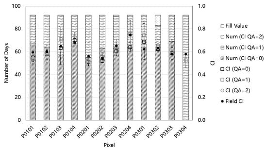
Figure 4.
MODIS monthly mean CIs calculated by daily CIs with different quality flags and the number of days of different quality flags for the twelve 500 m gridded pixels in the study area during the field observation period, i.e., from June to September 2018. The bar graph shows the number of different quality flags of the MODIS daily CIs, and the squares, diamonds and triangles represent the monthly average MODIS CIs calculated by the daily CIs with QA = 0, 1, and 2, respectively. The error bars represent the standard deviations of CIs with different quality flags. The black dots designate the field reference CIs scaled up from TRAC observations by the CLX method.
4.2. Validation of the MODIS CI Products
4.2.1. MODIS CIs vs. UAV CIs
As shown in Figure 5a, the RTCLSR BRDF model fits the UAV observations at different resolutions fairly well, and the root mean squared error (RMSE) reaches a minimum (~0.0002) at 70–80 m, up to a maximum (~0.0026) at 10 m. Multi-resolution UAV reflectances were obtained using the arithmetic average of observations surrounding the nadir point (Figure 1c). Although data at lower resolution tend to provide more stable multi-angle reflectance, as the error caused by the unstable attitude of the UVA can be smoothed by the aggregation process, satisfying the consistency of the VZA within the pixel is difficult to achieve with overly coarse resolutions of multi-angle reflectance. This occurs because the VZA discrepancy of the center and edge in the pixel with 100 m resolution can reach approximately 13°. Moreover, the observed reflectance near the direction of the darkspot (VZA = 32°) is almost the same as the modeled reflectance, whereas the observed reflectance near the direction of the hotspot (VZA = −30.7°) is smaller than the modeled reflectance, which can be attributed to the deviation of the direction between the observation VZA (−30.7°) and the SZA (32°). The BRFs in the hotspot, darkspot and CI directions at different resolutions based on the UAV observations and BRDF model data are shown in Figure 5b. Consistent with the results above, for different spatial resolutions from 10 m to 100 m, the BRFs in the direction of the darkspot essentially remain constant over different resolutions, whereas the BRFs in the direction of the hotspots decrease with increasing pixel resolution. Moreover, the CIs retrieved by using UAV observations and BRDF model data are almost the same, and both increase with increasing pixel resolution, which can be ascribed to the smoothing of the hotspot effect and thus the isotropic distribution of reflectances caused by the average aggregation in coarser resolution pixels.
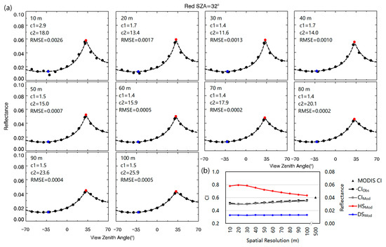
Figure 5.
Fitting UAV multi-angle reflectance data using the RTCLSR BRDF model and estimating UAV CIs of different spatial resolutions. (a) Fitting BRDF shapes of different resolution UAV reflectance data. The multi-angle observations are shown as black dots, and the reflectance values in the hotspot and darkspot directions of the BRDF models are marked as blue dots and red dots, respectively. The optimal values of C1 and C2 of the RTCLSR model are used to minimize the RMSE between the fitted BRDF and observed reflectance. (b) BRFs of hotspot (HSMod), darkspot (DSMod) and CIs calculated by using UAV observations (CIObs) and accordant RTCLSR model data (CIMod) in different spatial resolutions. The MODIS CI corresponds to the extent of the UAV observations.
Furthermore, the upscaled field CIs based on 30 m transect observations within the 100 m × 100 m UAV observation extent were obtained by the CLX and Avg methods (CICLX = CLAvg = 0.57), and the accordant 500 m resolution MODIS CI was calculated by using monthly (CI = 0.60, in August 2019) and daily (CI = 0.61, on 21 August 2019) data. As the quality of the MODIS daily CI was not the best (QA = 1), the MODIS monthly CI calculated by using the best quality data was used. The UAV CIs (CIObs = 0.56; CIMod = 0.55; at the 100 m scale) and upscale field CI are in good agreement with the UAV observations. The accordant 500 m resolution MODIS CI is slightly higher than the 100 m resolution UAV CI, but it tends to increase with increasing spatial resolution.
4.2.2. MODIS CIs vs. TRAC CIs
The validation result of the MODIS CI in the study area is shown in Figure 6, which is obtained by comparing the MODIS CI with the upscaled 500 m pixel-scale reference CIs obtained by using three upscaling strategies based on the TRAC measurements with 30 m transects. The 30 m CI maps obtained by using empirical transfer functions (TFs) and IDW interpolation methods are shown in Figure 6a,b, and the scatter plots of the two 30 m CI maps and field CIs with 30 m transects are shown in Figure 6c,d, respectively. Compared with the two 30 m CI maps, the one obtained by using the IDW interpolation method (Figure 6b,d) is more consistent with the field CIs (R = 0.97; RMSE = 0.02; bias = −0.0005), and there is no distinct variance in the accuracy of the CIs at the 30 m pixel scale among the different land cover types.
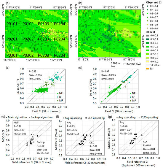
Figure 6.
Validation of the MODIS CI in the study area by using 500 m pixel-scale reference CIs scaled up from field observations by three different upscaling strategies. (a,b) show the 30 m CI maps of the study area by empirical transfer functions (TFs) and inverse distance weighting (IDW) methods based on field observations and Landsat 8 OLI surface reflectance data. (c,d) show the scatter plots of CIs in the above two 30 m CI maps and field observation CIs with 30 m transects, and the colors of the dots indicate different forest types. (e–g) display the validation results of the MODIS CI in the study area by comparing the MODIS CI and field reference CI at the 500 m pixel scale based on the three upscaling strategies. The MODIS CIs of the twelve pixels in the study area retrieved by the main and backup algorithms are compared with the field reference CIs in (e), and only the former are used in (f,g). The field reference CI in (e) is scaled up from the 30 m CI map by the Avg method, and the 30 m CI map is obtained by using the IDW interpolation method (b). The reference CIs in (f,g) are scaled up from field CIs with 30 m transects and the equivalent 500 m transects by using the Avg and CLX methods, and CIs with equivalent 500 m transects are calculated by integrating gap observations based on the TRAC measurements with 30 m transects. In (c–g), the black dashed line represents the 1:1 line, and the gray dashed lines represent the ±0.1 deviation lines.
As shown in the scatter plot of the CI map (Figure 6d), two 30 m NF pixels are overestimated because there is a path passing the observation sites, leading to small values of CI measurements, and two pixels are underestimated—one belonging to BF and the other belonging to MF—because there are coniferous forests surrounding the sites, leading to the lower values obtained by interpolation. The interpolation results are highly dependent on the surrounding observations, and 97% of the 30 m pixels of the CI map are calculated by observations within the range of 90 m. For the 30 m CI map obtained by using empirical transfer functions, this map shows a more homogeneous distribution of the CI in the study area, especially for the same land cover type (e.g., P0202), and its scatter plot has a relatively narrow range of 30 m pixel-scale CIs compared with field CIs, especially for the NF, which has a range of 0.4–0.7 for field CIs and narrows to 0.5–0.6 for 30 m pixel-scale CIs. The deviation between field CIs and the 30 m pixel-scale CIs estimated by the empirical transfer function method implies that reflectance data without multi-angle observations may be insufficient to retrieve vegetation structural characteristics because of the lack of knowledge of surface anisotropic properties. Consequently, the 30 m CI map obtained by the IDW method was used in the validation of the MODIS CI.
The validation results of the MODIS CI obtained by using 500 m pixel-scale reference CIs scaled up from field observations based on three upscaling strategies, including scaling up directly from TRAC CIs with 30 m transects and scaling up from 30 m CI maps and CIs with equivalent 500 m transects obtained by using field observations, are shown in Figure 6e–g. For the MODIS CIs of the twelve pixels in the study area, the monthly mean CIs in accordance with field observations (i.e., June to August) were used for validation to reduce the impact of the fill value and poor quality data of the daily CIs. The 500 m pixel-scale reference CIs scaled up from the 30 m CI map obtained by the IDW interpolation method were calculated by the Avg method and compared with the MODIS CIs retrieved by the main and backup algorithms (Figure 6e). Compared with the CIs based on the backup algorithm, the range of CIs calculated by the main algorithm is relatively narrow, and the CI values are lower but deviate less from the field CIs. The MODIS CIs retrieved by the backup algorithm correlate better with the field CIs, which is mainly due to the larger range of the retrieved CIs.
The field reference CIs scaled up from the TRAC CIs with 30 m transects and the equivalent 500 m transects are calculated by using the Avg and CLX methods (Figure 6f,g), and these data are compared with the MODIS CIs retrieved by main algorithm. The CIs with equivalent 500 m transects are obtained by integrating the gap observations of the TRAC measurements in the extent of the 500 m transects, and an average of 6 TRAC measurements are contained in one equivalent 500 m transect. Two to five equivalent 500 m transects are obtained in each 500 m gridded MODIS pixel according to the number of field observations within the pixel. The reference field CIs based on the 30 CI map are similar to the CIs scaled up from the 30 m transects by the Avg method, which reflects that the 30 CI map is in better agreement with the field observations. The 500 m pixel-scale reference CIs scaled up from the CIs with 30 m transects are lower than the CIs scaled up from the CIs with the equivalent 500 m transects, while these two data values are similar to the MODIS CIs. The higher CIs scaled up from CIs with equivalent 500 m transects can be attributed to the more heterogeneous distribution of leaves in the equivalent 500 m transects than in the 30 m transects in the study area.
The field reference CIs scaled up by the Avg method are greater than the CIs scaled up by the CLX method, and the MODIS CIs are more strongly correlated with the latter. Considering that the Avg method tends to smooth the variance of CIs in the upscaling pixels and thus leads to higher CIs, the CLX method is recommended in the upscaling of TRAC measured CIs. The overestimation of the Avg method in the upscaling of field CIs was also deduced in the analysis of UAV CIs in Section 4.2.1 and in previous studies conducted by Fang et al. [61] and Wei and Fang [21]. Compared with those in previous studies, the MODIS CIs in this validation framework are generally in better agreement with the validation data [20], as the field reference CIs at the 500 m pixel scale are much more comparable to the moderate-resolution products than the field CIs at the its original scale are.
4.3. Analysis of Subpixel CI Variations
4.3.1. Analysis Based on the TRAC CIs
To further understand the subpixel variance of CIs for moderate-resolution data and assess the possible validation uncertainties caused by the resolution deviations in the “point-to-pixel” comparison, the frequency density distribution of the difference between monthly MODIS CIs and CIs with 30 m transects as well as CIs with equivalent 500 m transects were analyzed for the twelve pixels. As shown in Figure 7, the discrepancies between the MODIS CIs and TRAC CIs are widest ranging from −0.5 to 0.5, which is a considerable error given that the CI varies from 0.33 to 1.0. If only one field observation is selected randomly that coincides with the 10th or 90th percentiles of the distribution, the MODIS-TRAC CI error can reach −0.27 or +0.18 on average for the CIs of the 30 m transects and −0.08 to 0.36 for the CIs of the equivalent 500 m transects. Approximately 54% of the CIs with 30 m transects were greater than the MODIS CI, and 73% of the CIs with the equivalent 500 m transects were less than the MODIS CI for an average of twelve pixels. CIs with equivalent 500 m transects that were calculated by integrating gap measurements were less than the CIs with 30 m transects overall, and the former showed a relatively narrow distribution. Both CIs within P0203 have relatively large ranges and dispersed distributions because of the heterogeneity of the surface. P0103, P0104 and P0204 also show relatively large ranges of MODIS-TRAC CI errors for the CIs of the 30 m transects, which may be attributed to the heterogeneous distribution of coniferous and non-coniferous forests within these pixels. The relatively rough terrain within these four pixels may also result in the higher variance of the TRAC CIs. P0204 shows a relatively concentrated distribution of the differences between MODIS CI and TRAC CIs with equivalent 500 m transects because this pixel contains less forestland area and only two CIs.
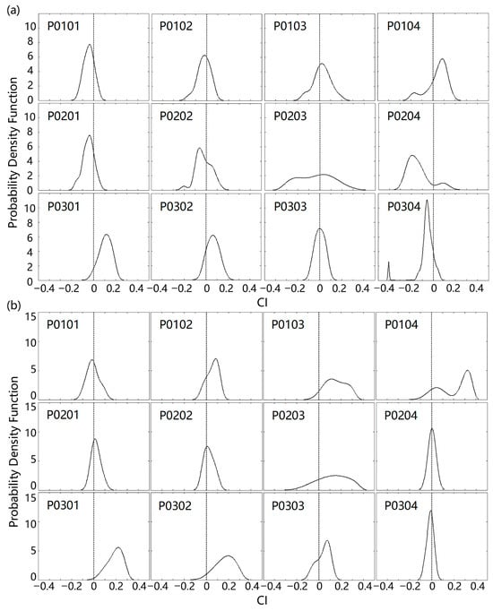
Figure 7.
Normalized frequency distributions of the MODIS CI minus (a) field CIs with 30 m transects and (b) CIs with equivalent 500 m transects for twelve 500 m gridded MODIS pixels in the study area. The vertical lines in the figure represent the points where the discrepancy between the MODIS CIs and the TRAC CIs is 0.
For the CIs with 30 m transects, if only one field observation was used for validation, the MODIS CIs are likely to be overestimated in P0103, P0104, P0301, and P0302, and underestimated in P0101, P0102, P0201, P0202, P0203, P0204 and P0304, whereas the MODIS CI in P0303 has the highest probability of obtaining a good evaluation result. Since the 500 m pixels always contain mixed information of multiple land cover types, the MODIS CIs of mixed pixels classified as coniferous tend to be less than the field CIs of non-coniferous pixels (i.e., P0101, P0102, P0201, and P0202), whereas the MODIS CIs of mixed pixels classified as non-coniferous pixels are prone to be greater than the measured CIs of coniferous pixels (i.e., P0103, P0104, P0301, and P0302). For P0204, most of the observed CIs of forest in this pixel are lower than the MODIS CI, as the pixel was classified as WSa because it contains approximately 53% of the GL, which has higher CIs. The observed CIs in P0203 show a relatively large range, while the MODIS CI is very close to its median. With respect to CIs with equivalent 500 m transects, except for P0101 and P0304, the MODIS CIs are likely overestimated in the remaining pixels, whereas the MODIS CIs of P0101, P0201, P0202, P0204, and P0304 are more likely to be evaluated as high quality data. CIs with equivalent 500 m transects integrated by using the gap measurements of 30 m transects tend to have a concentrated distribution of CI values for fewer CIs with longer transects. The distribution of gaps within the 30 m transect is relatively homogeneous in planted forests, whereas the integrated gaps of the equivalent 500 m transects are relatively heterogeneous, especially for forests with different tree species, which leads to smaller CIs for the equivalent 500 m transects.
4.3.2. Analysis Based on the 30 m CI Map
The semivariograms of twelve 500 m gridded MODIS pixels in the study area are estimated on the basis of the 30 m CI map using the interpolation method (Figure 8a and Table 1). P0203 has the highest sill and variance, which indicates a relatively heterogeneous distribution of CIs in this pixel, in line with the conclusions drawn from the subpixel variance analysis based on the TRAC CIs (Section 4.3.1). The semivariances of 30 m pixel-scale CIs in P0303 are not suitable for the spherical model. Although the CIs in this pixel show lower semivariances, the semivariance increases linearly without a plateau in the extent of the 500 m gridded pixel. As shown in Table 1, the order of the sills of these twelve pixels is almost the same as that of the variances, and the lower sills and variances represent more stable values of 30 m pixel-scale CIs within 500 m of the MODIS pixels. P0102, P0103 and P0204 have the same sills, while their ranges vary from 88.73 m to 276.21 m. P0103 has the smallest range (88.75 m), which indicates that the difference between the CIs of two locations more than approximately 90 m away will remain relatively stable, and field observations that can cover an extent greater than a circle with 90 m diameter are likely to validate the 500 m resolution CI data reasonably well. P0102 has the largest range of these three pixels, and the variance in range is highly dependent on the spatial pattern of the 30 m CIs within the pixels. Pixels with relatively even spatial patterns of CIs tend to obtain small ranges and thus can be evaluated by observations to a relatively small extent, and vice versa. In addition, P0101, P0201, P0202, and P0301 have relatively low sills and ranges, while P0104, P0304, and P0302 have relatively high sills and ranges. On average, except for P0303, the sill of all the eleven pixels is 0.006, and the range is 209 m. Moreover, the analysis of Section 4.2.1 partly confirms that the UAV CIs and MODIS CI become closer as the spatial resolution increases from 10 m to 100 m for the UAV CIs in P0202, which has a range of 163.54 m.
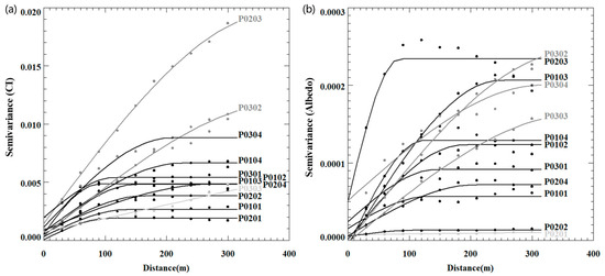
Figure 8.
Semivariograms with 30 m lags obtained by using a 30 m CI map (a) produced by the spatial interpolation method and a 30 m albedo map (b) derived from Landsat 8 OLI reference data of twelve 500 m gridded MODIS pixels in the study area. The dots present the calculated variogram estimators and the solid curves indicate the fitting semivariogram based on the spherical model by using 30 m maps of the 500 m pixel extent. The black symbols indicate that the range of semivariance for the pixel is less than 300 m, while the dark gray symbols indicate that the range is greater than 300 m, and the light gray symbols indicate that the spherical model is not fit for the pixel.

Table 1.
Characteristics of the 12 MODIS pixels and the related details. Num.: number of observations. MN: mean. Std: standard deviation. Avg and CLX indicate the two upscaling methods used to estimate the 500 m reference CIs: Avg is the arithmetic average; CLX is an aggregation of fine resolution pixels based on the CLX method. RF: random forest classification. LC: land cover. NF: needleleaf forests. BF: broadleaf forests. MF: mixed forests. GL: grasslands. WSa: woody savannas. “Maj.” denotes the most frequent land cover type of the MODIS IGBP data in the past 5 years, i.e., 2014–2018. “CI (Main)” and “CI (Backup)” represent the MODIS CIs derived from the main and backup algorithms, respectively. “QA” indicates the quality flag of the MODIS CI. Var.: variance. “Model Not Fit” indicates that the semivariance distribution is incompatible with the isotropic spherical model used in the semivariogram analysis.
The semivariograms obtained based on a 30 m albedo map based on Landsat 8 OLI surface reflectance data by using a widely used narrowband-to-broadband albedo conversion method [82,83] of the twelve 500 m gridded MODIS pixels in the study area are shown in Figure 8b. Compared with the semivariograms of the 30 m CI map (Figure 8 and Table 1), there is a similar order of heterogeneous distribution of subpixel variance for the twelve pixels. P0101, P0201 and P0202 have lower sills and ranges that mainly consist of NF; P0203, P0302 and P0304 have higher sills and ranges that contain different land cover types with relatively irregular distributions, and the others are in the middle. Compared with the albedo map, P0203 has a greater range in the CI map, which implies a more heterogeneous distribution of subpixel CIs than does the albedo map because the CI values of forests vary largely even for the same land cover type, while the albedo changes slightly. P0103 and P0303 show relatively high variances and heterogeneity in the 30 m albedo map compared with the CI map. Within these two pixels, the CIs of forestland area change slightly (Figure 6b), and the difference in albedo between forestland and GL in these pixels may be greater than that of the CIs. Consequently, the representative analysis of CI field observations using high-resolution albedo data can improve the reasonableness of the validation results to some extent, while high-resolution CI data can further specify the subpixel variance of CIs and thus improve the validation of moderate-resolution CI products.
5. Discussion
The TRAC instrument takes advantage of measurements along a transect of tens to hundreds of meters [18,72], which are considered the most appropriate field measurements for the validation of remote sensing data. Thirty-meter observation transects were used in this study to ensure that the transects were perpendicular to the sun. While grassland is too short to be measured by TRAC instruments, the average MODIS CIs of the GL pixels within the Luanhe River Basin are used as a priori knowledge of the GL CIs of 30 m pixels. This approximation introduces uncertainties to this study for the influence of the scale effect, terrain changes and surface heterogeneities, but the uncertainty is limited for the relatively constant value of the GL CIs on the global extent (~0.8) [20]. For the forest measurements, the needle-to-shoot ratio and woody-to-total area ratio of the similar tree species obtained from previous studies were used in the process of TRAC observations, which introduced errors to the validation [84]. Additionally, the TRAC CIs are increase with increasing solar zenith angle [18] and change with the observation height [12]. The field measurements in this study were conducted between 8:00 a.m. and 18:00 p.m., with an observation height of approximately 1 m, and further observations are needed to obtain more specific surface information and conduct further validations.
As for topographic influences, although field observations with slopes between 20–25° constitute less than 10% of the total, topography may introduce uncertainties in MODIS CI validation. In this study, TRAC transects were aligned along the slope direction to minimize topographic effects on canopy gap fraction observations. This approach limited the direct impact of terrain on in situ TRAC CIs. However, topography can influence vegetation growth patterns and distribution, leading to increased spatial heterogeneity of CI values. This is evidenced by the higher standard deviations in CI measurements from pixels P0104 and P0204 (Table 1; 0.09 and 0.10, respectively), where steeper slopes are predominantly concentrated. In terms of satellite-based CI retrieval, topography affects BRDF measurements and subsequent MODIS CI estimation. Compared to flat terrain, topographic shading enhances the reflectance contrast between hotspot and darkspot directions, potentially leading to underestimation of the retrieved CI [17,85]. The standard MODIS BRDF product used in this study is not explicitly corrected for topographic effects. In pixel P0204, the MODIS CI was underestimated (Table 1; ~0.1 lower) compared to the 500 m pixel-scale reference CIs scaled up from the 30 m CI map. P0104 exhibits a different pattern, with a slight overestimation of MODIS CI. This can be attributed to the dominance of coniferous forests (55% coverage), which typically exhibit higher clumping characteristics (lower CI values). The application of non-coniferous CI-NDHD retrieval algorithms at the MODIS pixel scale for the mixed forest cover resulted in an overestimate of MODIS CI [86,87], thereby counteracting the topographic influence in this pixel.
The accuracy of the MODIS CI product is inevitably affected by the upstream data. The MODIS BRDF product is produced by using pseudo-multi-angle reflectance data that is accumulated from 16-day observations and a semi-empirical kernel-driven BRDF model [81], and the quality of observations and the performance of the BRDF model are closely related to the accuracy of the CI retrievals. Thus, the quality flags of the CI product that take the BRDF quality flags into account should be fully considered in the applications. The land cover type data determine the crown shapes used to estimate the CIs, which influence the CI retrievals by using the CI–NDHD equations (main algorithm) and land cover type based LUT (backup algorithm). In this case study, the MODIS IGBP data of 2018 disagree with the field observations, and the domain land cover type of the past five years (2014–2018) shows limited improvement over the LC data of 2018, while the upscaled 30 m FROM-GLC data are relatively similar to the LC data from field observations at the 500 m pixel scale. Given that the NF has a special shoot structure and thus differs from the other land cover types in the retrievals, the errors in the main algorithm can reach 0.33 by confusing the NF with other land cove types. Therefore, caution should be taken when considering the influence of land cover types on CI retrievals in relevant analyses.
High-resolution remote sensing CI maps are urgently needed for the further validations and applications of CI data. This study produced 30 m resolution CI maps of the study area on the basis of substantial field measurements using the TF and IDW methods. The 30 m CI map deviated by the TF method presented a narrow range of values compared to that derived from the IDW method, particularly for the NF. This limitation may be attributed to the fact that the field observations used to derive the empirical transfer functions inadequately represented the full spectrum of canopy clumping conditions. Moreover, as the input data were predominantly collected from coniferous forests, which likely contributed to a suboptimal performance in the study area. However, the IDW method produced a more realistic distribution of CI values. This can be attributed to the relatively continuous and gradual variations in canopy structure and topography, combined with the availability of dense field measurements. Notably, 97% of the IDW-interpolated CI values were derived from field observations located within a three-pixel radius of the target location. Given its strong dependence on dense sampling, the IDW method should be applied with caution in regions with limited field campaigns. Furthermore, the Kriging interpolation method underperformed (R = 0.74; RMSE = 0.06; bias = −0.0005) compared to IDW in the study area. This is likely because the small-scale, high-density clustering of the field observations led to overfitting during the variogram fitting process.
Regarding CI retrieval algorithms, the predominant approach for existing products remains the CI–NDHD method. The acquisition of high-accuracy CI relies heavily on precise hotspot data, which is particularly challenging for the limited MODIS angular sampling. With the ongoing updates of MODIS products, future efforts could valuably explore CI retrievals using data from Visible Infrared Imaging Radiometer Suite (VIIRS) [88]. Similarly, deriving high-resolution CI maps is another promising direction. Such data would not only provide more detailed structural information but also serve as a crucial reference for validating moderate-resolution CI products. For instance, Zhao et al. [89] have demonstrated the potential of spaceborne LiDAR system for obtaining 30 m forest CI. Furthermore, the development of algorithms to retrieve CI from 10 m or higher-resolution satellite data constitutes a significant and necessary area for future research. Additionally, systematic and organized field campaigns for CI validation and further studies of the scale effect between field observations and satellite-based CI products will shed light on the extensive validation and application of CI.
6. Conclusions
This study developed a validation scheme by using multi-source data at multiple spatial scales, including field measurements, UAV observations, Landsat 8 OLI data and MODIS products. Three upscaling strategies were used to obtain 500 m pixel-scale reference CIs from field measurements, and multi-resolution CIs were calculated by UAV multi-angle reflectance; then, these data were used to validate the corresponding MODIS CIs, and the scale effect of the CI retrievals was explored. Transfer functions and interpolation methods were used to obtain a 30 m CI map with the upscaling strategies. These data and field observations were further used to analyze the subpixel variances within 500 m resolution pixels on the basis of the probability density function and semivariogram technique. Additionally, 30 m LC data and 5-year MODIS IGBP time series were used to assess the impacts of LC data on CI retrievals.
Through the validation scheme used in this case study, we found that the MODIS CIs were strongly correlated with the upscaled field CIs (R = 0.75; RMSE = 0.05; bias = 0.02 for the main algorithm; R = 0.80; RMSE = 0.06; bias = 0.05 for the backup algorithm), with higher RMSE and bias but lower R values than the stated accuracy of this product [20]. The narrow range of CIs in this study, consisting of relatively few land cover types compared with the global scale, led to a lower statistical significance for the correlation between the MODIS CIs and field reference CIs. The MODIS CI also showed good agreement with the UAV CI, which tended to increase with increasing pixel resolution. The average upscaling method overestimated the CIs at lower resolution, and CLX was a better choice for the upscaling of field CIs. In addition, field observations were used to assess the uncertainty of validation through direct comparisons between single-field observations and the MODIS CI. Further quantifying extreme cases (10th and 90th percentiles of the error probability density distributions) revealed that the average error can be as large as −0.21 or +0.27, which is a considerable error given that CIs vary from 0.33 to 1.0. Moreover, a variogram analysis using a 30 m CI map revealed that the average observational footprint needed for a spatially representative sample was approximately 209 m for these twelve pixels, which highlights the importance of determining the subpixel variance for validation between satellite retrievals and in situ measurements. In addition, we analyzed the influence of LC and BRDF data on the derivation of the CI. The mismatch of LC data could cause up to 0.33 error in the estimation of the CI for the main algorithm, and CIs derived from the best quality BRDF data through the main algorithm (QA = 0) were recommended for relevant applications.
This study demonstrates a promising multi-scale approach for validating moderate-resolution CI products, with a specific focus on the upscaling field observations to high-to-moderate satellite pixel resolutions and the associated scale effect arising from surface heterogeneity. However, the extensive validation of satellite-based global CI products remains challenging because of the lack of well-organized field observations with globally representative locations and temporal coverage for systematic validation [90]. Furthermore, high-resolution CI maps are urgently needed to provide detailed structural information and to serve as a crucial validation benchmark for moderate-resolution products.
Author Contributions
Conceptualization, Z.J. and S.Y.; methodology, Z.J., Y.D. and L.C.; software, A.D. and X.Z.; validation, S.Y. and Z.J.; formal analysis, S.Y. and Z.J.; investigation, J.G., R.X., Y.T., Z.Z., S.L. and C.W.; resources, Z.J.; data curation, F.Q., Q.Z. and Y.Z.; writing—original draft preparation, S.Y.; writing—review and editing, Z.J.; visualization, S.Y.; supervision, Z.J. and Y.D.; project administration, Z.J.; funding acquisition, Z.J. and J.J. All authors have read and agreed to the published version of the manuscript.
Funding
This research was funded by the National Natural Science Foundation of China (No. 42471352), the Major Program of the Natural Science Foundation of China (No. 42090013), the National Natural Science Foundation of China (No. 41971288) and the Beijing Natural Science Foundation (No. QY25415).
Data Availability Statement
The MODIS BRDF/Albedo Model Parameter product and Land Cover product with a spatial resolution of 500 m can be downloaded from https://lpdaac.usgs.gov/product_search/?view=cards&sort=title, accessed on 9 August 2025. The 30 m Finer Resolution Observation and Monitoring Global Land Cover (FROM-GLC) version 2 (2015_v1) data can be downloaded from https://data-starcloud.pcl.ac.cn/, accessed on 9 August 2025. The MODIS CI data can be downloaded from https://www.geodata.cn/data/datadetails.html?dataguid=214951029475816&docid=7534, accessed on 9 August 2025. The Landsat 8 Surface Reflectance data can be downloaded from https://espa.cr.usgs.gov/, accessed on 9 August 2025.
Acknowledgments
The MODIS data were obtained from the NASA EOSDIS Land Processes Distributed Active Archive Center (LP DAAC). The Landsat 8 data were obtained from the U.S. Geological Survey (USGS) Earth Resources Observation and Science (EROS) Center Science Processing Architecture (ESPA). The Finer Resolution Observation and Monitoring Global Land Cover (FROM-GLC) version 2 (2015_v1) data were obtained from the Star Cloud Data Service Platform. The Shuttle Radar Topography Mission (SRTM) Digital Elevation Model (DEM) data were obtained from the National Aeronautics and Space Administration (NASA) and the National Geospatial-Intelligence Agency (NGA—previously known as the National Imagery and Mapping Agency, or NIMA). The Sentinel-2B Level 1C data were obtained from the European Space Agency (ESA).
Conflicts of Interest
The authors declare no conflicts of interest.
Appendix A
Table A1.
Field observations conducted in the Matikeng forest district of Saihanba National Forest Park, Hebei, China. during 12–15 June and 24–31 August. Num.: number of observations. LC: land cover. DNF: deciduous needleleaf forests. DBF: deciduous broadleaf forests. MF: mixed forests. ENF: evergreen needleleaf forests. CI: clumping index.
| Num. | Longitude | Latitude | LC | CI | Date |
|---|---|---|---|---|---|
| 1 | 117.3170 | 42.4089 | DNF | 0.43 | 12 June 2018 |
| 2 | 117.3170 | 42.4095 | DNF | 0.48 | 12 June 2018 |
| 3 | 117.3170 | 42.4098 | DNF | 0.46 | 12 June 2018 |
| 4 | 117.3167 | 42.4101 | DNF | 0.44 | 12 June 2018 |
| 5 | 117.3162 | 42.4103 | DNF | 0.53 | 12 June 2018 |
| 6 | 117.3124 | 42.4124 | DNF | 0.59 | 13 June 2018 |
| 7 | 117.3124 | 42.4114 | DNF | 0.54 | 13 June 2018 |
| 8 | 117.3130 | 42.4108 | DNF | 0.55 | 13 June 2018 |
| 9 | 117.3142 | 42.4112 | DNF | 0.66 | 13 June 2018 |
| 10 | 117.3141 | 42.4104 | DNF | 0.47 | 13 June 2018 |
| 11 | 117.3130 | 42.4103 | DNF | 0.53 | 13 June 2018 |
| 12 | 117.3119 | 42.4103 | DNF | 0.60 | 13 June 2018 |
| 13 | 117.3112 | 42.4097 | DNF | 0.55 | 13 June 2018 |
| 14 | 117.3118 | 42.4111 | DNF | 0.68 | 13 June 2018 |
| 15 | 117.3150 | 42.4106 | DNF | 0.59 | 13 June 2018 |
| 16 | 117.3148 | 42.4115 | DNF | 0.60 | 13 June 2018 |
| 17 | 117.3149 | 42.4124 | DNF | 0.46 | 13 June 2018 |
| 18 | 117.3155 | 42.4129 | DNF | 0.55 | 13 June 2018 |
| 19 | 117.3145 | 42.4131 | DNF | 0.58 | 13 June 2018 |
| 20 | 117.3128 | 42.4123 | DNF | 0.65 | 13 June 2018 |
| 21 | 117.3129 | 42.4096 | DNF | 0.55 | 14 June 2018 |
| 22 | 117.3135 | 42.4094 | DNF | 0.60 | 14 June 2018 |
| 23 | 117.3143 | 42.4093 | DNF | 0.57 | 14 June 2018 |
| 24 | 117.3201 | 42.4125 | DNF | 0.60 | 14 June 2018 |
| 25 | 117.3193 | 42.4123 | DNF | 0.59 | 14 June 2018 |
| 26 | 117.3187 | 42.4125 | DNF | 0.59 | 14 June 2018 |
| 27 | 117.3188 | 42.4117 | DNF | 0.59 | 14 June 2018 |
| 28 | 117.3175 | 42.4113 | DNF | 0.59 | 14 June 2018 |
| 29 | 117.3167 | 42.4120 | DNF | 0.61 | 14 June 2018 |
| 30 | 117.3161 | 42.4126 | DNF | 0.56 | 14 June 2018 |
| 31 | 117.3161 | 42.4114 | DNF | 0.59 | 14 June 2018 |
| 32 | 117.3175 | 42.4109 | DNF | 0.54 | 14 June 2018 |
| 33 | 117.3182 | 42.4106 | DNF | 0.51 | 14 June 2018 |
| 34 | 117.3183 | 42.4100 | DNF | 0.51 | 14 June 2018 |
| 35 | 117.3191 | 42.4096 | DNF | 0.48 | 14 June 2018 |
| 36 | 117.3187 | 42.4091 | DNF | 0.57 | 14 June 2018 |
| 37 | 117.3194 | 42.4096 | DNF | 0.58 | 14 June 2018 |
| 38 | 117.3194 | 42.4104 | DNF | 0.58 | 14 June 2018 |
| 39 | 117.3189 | 42.4106 | DNF | 0.61 | 14 June 2018 |
| 40 | 117.3189 | 42.4114 | DNF | 0.61 | 14 June 2018 |
| 41 | 117.3203 | 42.4129 | DNF | 0.61 | 14 June 2018 |
| 42 | 117.3211 | 42.4128 | DNF | 0.63 | 14 June 2018 |
| 43 | 117.3217 | 42.4123 | DNF | 0.55 | 14 June 2018 |
| 44 | 117.3226 | 42.4121 | DNF | 0.45 | 14 June 2018 |
| 45 | 117.3214 | 42.4115 | DNF | 0.46 | 14 June 2018 |
| 46 | 117.3207 | 42.4117 | DNF | 0.72 | 14 June 2018 |
| 47 | 117.3205 | 42.4112 | DNF | 0.50 | 14 June 2018 |
| 48 | 117.3210 | 42.4108 | DNF | 0.50 | 14 June 2018 |
| 49 | 117.3213 | 42.4104 | DNF | 0.47 | 14 June 2018 |
| 50 | 117.3204 | 42.4100 | DNF | 0.48 | 14 June 2018 |
| 51 | 117.3205 | 42.4104 | DNF | 0.58 | 14 June 2018 |
| 52 | 117.3207 | 42.4087 | DNF | 0.60 | 14 June 2018 |
| 53 | 117.3207 | 42.4085 | DNF | 0.33 | 14 June 2018 |
| 54 | 117.3220 | 42.4099 | DNF | 0.63 | 14 June 2018 |
| 55 | 117.3218 | 42.4105 | DBF | 0.90 | 14 June 2018 |
| 56 | 117.3223 | 42.4111 | DNF | 0.59 | 14 June 2018 |
| 57 | 117.3227 | 42.4115 | DNF | 0.58 | 14 June 2018 |
| 58 | 117.3236 | 42.4110 | DNF | 0.63 | 14 June 2018 |
| 59 | 117.3238 | 42.4113 | MF | 0.79 | 14 June 2018 |
| 60 | 117.3189 | 42.4044 | DNF | 0.54 | 24 August 2018 |
| 61 | 117.3192 | 42.4050 | DNF | 0.48 | 24 August 2018 |
| 62 | 117.3197 | 42.4047 | DNF | 0.52 | 24 August 2018 |
| 63 | 117.3178 | 42.4044 | DNF | 0.55 | 24 August 2018 |
| 64 | 117.3175 | 42.4044 | DNF | 0.58 | 24 August 2018 |
| 65 | 117.3167 | 42.4044 | DNF | 0.62 | 24 August 2018 |
| 66 | 117.3161 | 42.4044 | DNF | 0.58 | 24 August 2018 |
| 67 | 117.3150 | 42.4044 | DNF | 0.54 | 24 August 2018 |
| 68 | 117.3156 | 42.4050 | DNF | 0.59 | 24 August 2018 |
| 69 | 117.3167 | 42.4056 | DNF | 0.60 | 24 August 2018 |
| 70 | 117.3179 | 42.4061 | DNF | 0.55 | 24 August 2018 |
| 71 | 117.3178 | 42.4050 | DNF | 0.60 | 24 August 2018 |
| 72 | 117.3191 | 42.4052 | DNF | 0.66 | 24 August 2018 |
| 73 | 117.3203 | 42.4050 | DNF | 0.57 | 24 August 2018 |
| 74 | 117.3208 | 42.4056 | DBF | 0.93 | 24 August 2018 |
| 75 | 117.3208 | 42.4061 | DNF | 0.58 | 24 August 2018 |
| 76 | 117.3206 | 42.4064 | DNF | 0.57 | 24 August 2018 |
| 77 | 117.3181 | 42.4056 | DNF | 0.60 | 24 August 2018 |
| 78 | 117.3175 | 42.4056 | DNF | 0.60 | 24 August 2018 |
| 79 | 117.3169 | 42.4064 | DNF | 0.60 | 24 August 2018 |
| 80 | 117.3169 | 42.4069 | DNF | 0.58 | 24 August 2018 |
| 81 | 117.3183 | 42.4069 | DNF | 0.51 | 24 August 2018 |
| 82 | 117.3186 | 42.4067 | DNF | 0.50 | 24 August 2018 |
| 83 | 117.3194 | 42.4067 | DNF | 0.53 | 24 August 2018 |
| 84 | 117.3197 | 42.4058 | DNF | 0.63 | 24 August 2018 |
| 85 | 117.3211 | 42.4064 | DNF | 0.58 | 24 August 2018 |
| 86 | 117.3211 | 42.4069 | DNF | 0.58 | 24 August 2018 |
| 87 | 117.3208 | 42.4075 | DNF | 0.57 | 24 August 2018 |
| 88 | 117.3217 | 42.4072 | DNF | 0.58 | 24 August 2018 |
| 89 | 117.3208 | 42.4078 | DNF | 0.60 | 24 August 2018 |
| 90 | 117.3194 | 42.4078 | DNF | 0.55 | 24 August 2018 |
| 91 | 117.3186 | 42.4081 | DNF | 0.61 | 24 August 2018 |
| 92 | 117.3183 | 42.4081 | DNF | 0.56 | 24 August 2018 |
| 93 | 117.3175 | 42.4083 | DNF | 0.53 | 24 August 2018 |
| 94 | 117.3164 | 42.4078 | DNF | 0.54 | 24 August 2018 |
| 95 | 117.3156 | 42.4075 | DNF | 0.53 | 24 August 2018 |
| 96 | 117.3164 | 42.4072 | DNF | 0.57 | 24 August 2018 |
| 97 | 117.3175 | 42.4072 | DNF | 0.60 | 24 August 2018 |
| 98 | 117.3192 | 42.4075 | DNF | 0.55 | 24 August 2018 |
| 99 | 117.3186 | 42.4089 | DNF | 0.54 | 24 August 2018 |
| 100 | 117.3194 | 42.4086 | DNF | 0.45 | 25 August 2018 |
| 101 | 117.3203 | 42.4092 | DNF | 0.63 | 25 August 2018 |
| 102 | 117.3206 | 42.4094 | DBF | 0.77 | 25 August 2018 |
| 103 | 117.3214 | 42.4089 | DNF | 0.56 | 25 August 2018 |
| 104 | 117.3222 | 42.4097 | DNF | 0.60 | 25 August 2018 |
| 105 | 117.3228 | 42.4097 | DBF | 0.82 | 25 August 2018 |
| 106 | 117.3236 | 42.4094 | DBF | 0.84 | 25 August 2018 |
| 107 | 117.3250 | 42.4094 | DBF | 0.86 | 25 August 2018 |
| 108 | 117.3253 | 42.4094 | DBF | 0.87 | 25 August 2018 |
| 109 | 117.3272 | 42.4094 | MF | 0.78 | 25 August 2018 |
| 110 | 117.3281 | 42.4094 | DBF | 0.76 | 25 August 2018 |
| 111 | 117.3289 | 42.4097 | DBF | 0.77 | 25 August 2018 |
| 112 | 117.3300 | 42.4106 | DBF | 0.84 | 25 August 2018 |
| 113 | 117.3289 | 42.4106 | DNF | 0.53 | 25 August 2018 |
| 114 | 117.3283 | 42.4100 | DNF | 0.58 | 25 August 2018 |
| 115 | 117.3261 | 42.4100 | MF | 0.91 | 25 August 2018 |
| 116 | 117.3253 | 42.4100 | DBF | 0.78 | 25 August 2018 |
| 117 | 117.3242 | 42.4103 | DBF | 0.82 | 25 August 2018 |
| 118 | 117.3228 | 42.4106 | DBF | 0.75 | 25 August 2018 |
| 119 | 117.3208 | 42.4100 | MF | 0.86 | 25 August 2018 |
| 120 | 117.3289 | 42.4108 | MF | 0.70 | 25 August 2018 |
| 121 | 117.3286 | 42.4106 | DBF | 0.84 | 25 August 2018 |
| 122 | 117.3281 | 42.4108 | DBF | 0.74 | 25 August 2018 |
| 123 | 117.3272 | 42.4108 | MF | 0.81 | 25 August 2018 |
| 124 | 117.3267 | 42.4108 | DBF | 0.85 | 25 August 2018 |
| 125 | 117.3264 | 42.4111 | DBF | 0.86 | 25 August 2018 |
| 126 | 117.3256 | 42.4111 | DBF | 0.83 | 25 August 2018 |
| 127 | 117.3253 | 42.4111 | DBF | 0.71 | 25 August 2018 |
| 128 | 117.3244 | 42.4111 | MF | 0.78 | 25 August 2018 |
| 129 | 117.3242 | 42.4108 | DBF | 0.80 | 25 August 2018 |
| 130 | 117.3214 | 42.4136 | DNF | 0.54 | 25 August 2018 |
| 131 | 117.3217 | 42.4133 | DNF | 0.60 | 25 August 2018 |
| 132 | 117.3219 | 42.4128 | DNF | 0.59 | 25 August 2018 |
| 133 | 117.3219 | 42.4133 | DNF | 0.58 | 25 August 2018 |
| 134 | 117.3203 | 42.4144 | DNF | 0.57 | 25 August 2018 |
| 135 | 117.3197 | 42.4144 | DNF | 0.61 | 25 August 2018 |
| 136 | 117.3189 | 42.4142 | DNF | 0.55 | 25 August 2018 |
| 137 | 117.3178 | 42.4139 | DNF | 0.53 | 25 August 2018 |
| 138 | 117.3172 | 42.4142 | DNF | 0.52 | 25 August 2018 |
| 139 | 117.3158 | 42.4139 | DNF | 0.64 | 25 August 2018 |
| 140 | 117.3153 | 42.4142 | DNF | 0.58 | 25 August 2018 |
| 141 | 117.3158 | 42.4133 | DNF | 0.63 | 25 August 2018 |
| 142 | 117.3167 | 42.4136 | DNF | 0.59 | 25 August 2018 |
| 143 | 117.3178 | 42.4133 | DNF | 0.63 | 25 August 2018 |
| 144 | 117.3181 | 42.4131 | DNF | 0.59 | 25 August 2018 |
| 145 | 117.3194 | 42.4136 | DNF | 0.63 | 25 August 2018 |
| 146 | 117.3169 | 42.4147 | DNF | 0.52 | 27 August 2018 |
| 147 | 117.3172 | 42.4150 | DNF | 0.51 | 27 August 2018 |
| 148 | 117.3172 | 42.4147 | DNF | 0.62 | 27 August 2018 |
| 149 | 117.3181 | 42.4147 | DNF | 0.55 | 27 August 2018 |
| 150 | 117.3194 | 42.4150 | DNF | 0.59 | 27 August 2018 |
| 151 | 117.3200 | 42.4153 | DNF | 0.56 | 27 August 2018 |
| 152 | 117.3203 | 42.4147 | DNF | 0.60 | 27 August 2018 |
| 153 | 117.3206 | 42.4156 | DNF | 0.58 | 27 August 2018 |
| 154 | 117.3214 | 42.4142 | DNF | 0.56 | 27 August 2018 |
| 155 | 117.3211 | 42.4153 | DNF | 0.65 | 27 August 2018 |
| 156 | 117.3203 | 42.4158 | DNF | 0.56 | 27 August 2018 |
| 157 | 117.3200 | 42.4164 | DNF | 0.67 | 27 August 2018 |
| 158 | 117.3197 | 42.4165 | DNF | 0.64 | 27 August 2018 |
| 159 | 117.3194 | 42.4161 | MF | 0.69 | 27 August 2018 |
| 160 | 117.3214 | 42.4158 | DNF | 0.59 | 27 August 2018 |
| 161 | 117.3222 | 42.4158 | DNF | 0.61 | 27 August 2018 |
| 162 | 117.3231 | 42.4156 | DNF | 0.59 | 27 August 2018 |
| 163 | 117.3242 | 42.4158 | MF | 0.69 | 27 August 2018 |
| 164 | 117.3239 | 42.4161 | DNF | 0.62 | 27 August 2018 |
| 165 | 117.3236 | 42.4164 | DNF | 0.57 | 27 August 2018 |
| 166 | 117.3231 | 42.4164 | MF | 0.66 | 27 August 2018 |
| 167 | 117.3217 | 42.4164 | MF | 0.65 | 27 August 2018 |
| 168 | 117.3133 | 42.4128 | DNF | 0.60 | 29 August 2018 |
| 169 | 117.3133 | 42.4122 | DNF | 0.56 | 29 August 2018 |
| 170 | 117.3139 | 42.4125 | DNF | 0.51 | 29 August 2018 |
| 171 | 117.3131 | 42.4114 | DNF | 0.55 | 29 August 2018 |
| 172 | 117.3114 | 42.4117 | DNF | 0.60 | 29 August 2018 |
| 173 | 117.3118 | 42.4122 | DNF | 0.52 | 29 August 2018 |
| 174 | 117.3106 | 42.4111 | DNF | 0.55 | 29 August 2018 |
| 175 | 117.3108 | 42.4108 | DNF | 0.48 | 29 August 2018 |
| 176 | 117.3106 | 42.4106 | DNF | 0.58 | 29 August 2018 |
| 177 | 117.3106 | 42.4103 | DNF | 0.53 | 29 August 2018 |
| 178 | 117.3106 | 42.4100 | DNF | 0.55 | 29 August 2018 |
| 179 | 117.3103 | 42.4094 | DNF | 0.49 | 29 August 2018 |
| 180 | 117.3086 | 42.4094 | DNF | 0.58 | 29 August 2018 |
| 181 | 117.3072 | 42.4092 | DNF | 0.60 | 29 August 2018 |
| 182 | 117.3079 | 42.4102 | DNF | 0.51 | 29 August 2018 |
| 183 | 117.3085 | 42.4105 | DNF | 0.56 | 29 August 2018 |
| 184 | 117.3069 | 42.4089 | DNF | 0.58 | 29 August 2018 |
| 185 | 117.3064 | 42.4086 | DNF | 0.56 | 29 August 2018 |
| 186 | 117.3069 | 42.4086 | DNF | 0.54 | 29 August 2018 |
| 187 | 117.3075 | 42.4089 | DNF | 0.52 | 29 August 2018 |
| 188 | 117.3086 | 42.4089 | DNF | 0.50 | 29 August 2018 |
| 189 | 117.3083 | 42.4086 | DNF | 0.60 | 29 August 2018 |
| 190 | 117.3094 | 42.4086 | DNF | 0.62 | 29 August 2018 |
| 191 | 117.3100 | 42.4089 | DNF | 0.55 | 29 August 2018 |
| 192 | 117.3114 | 42.4089 | DNF | 0.57 | 29 August 2018 |
| 193 | 117.3117 | 42.4083 | DNF | 0.61 | 29 August 2018 |
| 194 | 117.3125 | 42.4083 | DNF | 0.50 | 29 August 2018 |
| 195 | 117.3131 | 42.4089 | DNF | 0.40 | 29 August 2018 |
| 196 | 117.3142 | 42.4089 | DNF | 0.56 | 29 August 2018 |
| 197 | 117.3144 | 42.4083 | DNF | 0.57 | 29 August 2018 |
| 198 | 117.3150 | 42.4083 | DNF | 0.47 | 29 August 2018 |
| 199 | 117.3164 | 42.4061 | DNF | 0.61 | 29 August 2018 |
| 200 | 117.3156 | 42.4056 | DNF | 0.62 | 29 August 2018 |
| 201 | 117.3142 | 42.4050 | DNF | 0.52 | 29 August 2018 |
| 202 | 117.3139 | 42.4047 | DNF | 0.59 | 29 August 2018 |
| 203 | 117.3131 | 42.4047 | DNF | 0.65 | 29 August 2018 |
| 204 | 117.3125 | 42.4047 | DNF | 0.55 | 29 August 2018 |
| 205 | 117.3114 | 42.4050 | DNF | 0.65 | 29 August 2018 |
| 206 | 117.3122 | 42.4050 | DNF | 0.62 | 29 August 2018 |
| 207 | 117.3131 | 42.4056 | DNF | 0.66 | 29 August 2018 |
| 208 | 117.3136 | 42.4064 | DNF | 0.58 | 29 August 2018 |
| 209 | 117.3144 | 42.4069 | DNF | 0.62 | 29 August 2018 |
| 210 | 117.3144 | 42.4075 | DNF | 0.54 | 29 August 2018 |
| 211 | 117.3150 | 42.4078 | DNF | 0.59 | 29 August 2018 |
| 212 | 117.3144 | 42.4081 | DNF | 0.58 | 29 August 2018 |
| 213 | 117.3136 | 42.4075 | DNF | 0.61 | 29 August 2018 |
| 214 | 117.3128 | 42.4072 | DNF | 0.54 | 29 August 2018 |
| 215 | 117.3117 | 42.4067 | DNF | 0.57 | 29 August 2018 |
| 216 | 117.3111 | 42.4064 | DNF | 0.60 | 29 August 2018 |
| 217 | 117.3106 | 42.4056 | DNF | 0.64 | 29 August 2018 |
| 218 | 117.3106 | 42.4053 | DNF | 0.61 | 29 August 2018 |
| 219 | 117.3089 | 42.4058 | DNF | 0.62 | 29 August 2018 |
| 220 | 117.3108 | 42.4061 | DNF | 0.52 | 29 August 2018 |
| 221 | 117.3114 | 42.4061 | DNF | 0.57 | 29 August 2018 |
| 222 | 117.3122 | 42.4064 | DNF | 0.57 | 29 August 2018 |
| 223 | 117.3131 | 42.4072 | DNF | 0.55 | 29 August 2018 |
| 224 | 117.3139 | 42.4075 | DNF | 0.60 | 29 August 2018 |
| 225 | 117.3144 | 42.4081 | DNF | 0.62 | 29 August 2018 |
| 226 | 117.3131 | 42.4081 | DNF | 0.56 | 29 August 2018 |
| 227 | 117.3131 | 42.4078 | DNF | 0.57 | 29 August 2018 |
| 228 | 117.3125 | 42.4075 | DNF | 0.64 | 29 August 2018 |
| 229 | 117.3117 | 42.4072 | DNF | 0.56 | 29 August 2018 |
| 230 | 117.3111 | 42.4067 | DNF | 0.45 | 29 August 2018 |
| 231 | 117.3106 | 42.4061 | DNF | 0.65 | 29 August 2018 |
| 232 | 117.3094 | 42.4058 | DNF | 0.54 | 29 August 2018 |
| 233 | 117.3092 | 42.4058 | DNF | 0.55 | 29 August 2018 |
| 234 | 117.3103 | 42.4067 | DNF | 0.50 | 30 August 2018 |
| 235 | 117.3100 | 42.4067 | DNF | 0.53 | 30 August 2018 |
| 236 | 117.3106 | 42.4078 | DNF | 0.51 | 30 August 2018 |
| 237 | 117.3094 | 42.4078 | DNF | 0.50 | 30 August 2018 |
| 238 | 117.3089 | 42.4078 | DNF | 0.53 | 30 August 2018 |
| 239 | 117.3083 | 42.4075 | DNF | 0.57 | 30 August 2018 |
| 240 | 117.3078 | 42.4072 | DNF | 0.62 | 30 August 2018 |
| 241 | 117.3067 | 42.4069 | DNF | 0.59 | 30 August 2018 |
| 241 | 117.3067 | 42.4069 | DNF | 0.59 | 30 August 2018 |
| 242 | 117.3058 | 42.4061 | DNF | 0.51 | 30 August 2018 |
| 243 | 117.3056 | 42.4058 | DNF | 0.62 | 30 August 2018 |
| 244 | 117.3047 | 42.4058 | DNF | 0.50 | 30 August 2018 |
| 245 | 117.3053 | 42.4064 | DNF | 0.57 | 30 August 2018 |
| 246 | 117.3058 | 42.4067 | MF | 0.61 | 30 August 2018 |
| 247 | 117.3064 | 42.4072 | DNF | 0.53 | 30 August 2018 |
| 248 | 117.3078 | 42.4078 | DNF | 0.53 | 30 August 2018 |
| 249 | 117.3081 | 42.4078 | DNF | 0.58 | 30 August 2018 |
| 250 | 117.3075 | 42.4078 | DNF | 0.53 | 30 August 2018 |
| 251 | 117.3067 | 42.4078 | DNF | 0.54 | 30 August 2018 |
| 252 | 117.3058 | 42.4072 | DNF | 0.60 | 30 August 2018 |
| 253 | 117.3053 | 42.4067 | ENF | 0.63 | 30 August 2018 |
| 254 | 117.3042 | 42.4058 | DNF | 0.59 | 30 August 2018 |
| 255 | 117.3031 | 42.4058 | DNF | 0.56 | 30 August 2018 |
| 256 | 117.3025 | 42.4061 | DNF | 0.56 | 30 August 2018 |
| 257 | 117.3031 | 42.4067 | ENF | 0.59 | 30 August 2018 |
| 258 | 117.3036 | 42.4072 | ENF | 0.51 | 30 August 2018 |
| 259 | 117.3044 | 42.4075 | DNF | 0.66 | 30 August 2018 |
| 260 | 117.3053 | 42.4078 | DNF | 0.49 | 30 August 2018 |
| 261 | 117.3039 | 42.4075 | DNF | 0.60 | 30 August 2018 |
| 262 | 117.3025 | 42.4069 | DNF | 0.65 | 30 August 2018 |
| 263 | 117.3019 | 42.4064 | DNF | 0.53 | 30 August 2018 |
| 264 | 117.3011 | 42.4058 | DNF | 0.56 | 30 August 2018 |
| 265 | 117.3 | 42.4056 | DNF | 0.68 | 30 August 2018 |
| 266 | 117.2997 | 42.4056 | DNF | 0.59 | 30 August 2018 |
| 267 | 117.2986 | 42.4044 | DNF | 0.69 | 30 August 2018 |
| 268 | 117.2986 | 42.4042 | MF | 0.63 | 30 August 2018 |
| 269 | 117.3303 | 42.4142 | DNF | 0.59 | 30 August 2018 |
| 270 | 117.3294 | 42.4139 | DNF | 0.65 | 30 August 2018 |
| 271 | 117.3286 | 42.4142 | DNF | 0.45 | 30 August 2018 |
| 272 | 117.3289 | 42.4144 | DNF | 0.68 | 30 August 2018 |
| 273 | 117.33 | 42.4153 | DNF | 0.62 | 30 August 2018 |
| 274 | 117.3311 | 42.4153 | MF | 0.75 | 30 August 2018 |
| 275 | 117.3319 | 42.4161 | MF | 0.77 | 30 August 2018 |
| 276 | 117.3322 | 42.4161 | DNF | 0.51 | 30 August 2018 |
| 277 | 117.3317 | 42.4164 | MF | 0.64 | 30 August 2018 |
| 278 | 117.3301 | 42.4166 | DNF | 0.64 | 30 August 2018 |
| 279 | 117.3289 | 42.4164 | DNF | 0.53 | 30 August 2018 |
| 280 | 117.3281 | 42.4164 | DNF | 0.52 | 30 August 2018 |
| 281 | 117.3267 | 42.4164 | DNF | 0.63 | 30 August 2018 |
| 282 | 117.3258 | 42.4164 | DNF | 0.53 | 30 August 2018 |
| 283 | 117.3261 | 42.4161 | DNF | 0.60 | 30 August 2018 |
| 284 | 117.3272 | 42.4156 | MF | 0.64 | 30 August 2018 |
| 285 | 117.3286 | 42.4156 | DNF | 0.55 | 30 August 2018 |
| 286 | 117.33 | 42.4156 | DNF | 0.58 | 30 August 2018 |
| 287 | 117.3297 | 42.415 | DNF | 0.56 | 30 August 2018 |
| 288 | 117.3294 | 42.4142 | DNF | 0.52 | 30 August 2018 |
| 289 | 117.3289 | 42.4142 | DNF | 0.67 | 30 August 2018 |
| 290 | 117.3281 | 42.4136 | DNF | 0.59 | 30 August 2018 |
| 291 | 117.3269 | 42.4142 | DNF | 0.63 | 30 August 2018 |
| 292 | 117.3269 | 42.4147 | MF | 0.74 | 30 August 2018 |
| 293 | 117.3275 | 42.415 | MF | 0.59 | 30 August 2018 |
| 294 | 117.3261 | 42.415 | MF | 0.65 | 30 August 2018 |
| 295 | 117.3256 | 42.4147 | MF | 0.65 | 30 August 2018 |
| 296 | 117.3244 | 42.4147 | DNF | 0.57 | 30 August 2018 |
| 297 | 117.3353 | 42.4133 | DNF | 0.60 | 31 August 2018 |
| 298 | 117.3361 | 42.4136 | DNF | 0.65 | 31 August 2018 |
| 299 | 117.3375 | 42.4142 | DNF | 0.59 | 31 August 2018 |
| 300 | 117.3383 | 42.415 | MF | 0.89 | 31 August 2018 |
| 301 | 117.3389 | 42.415 | DNF | 0.64 | 31 August 2018 |
| 302 | 117.3397 | 42.4161 | DBF | 0.85 | 31 August 2018 |
| 303 | 117.3405 | 42.4166 | DBF | 0.78 | 31 August 2018 |
| 304 | 117.3394 | 42.4161 | DBF | 0.73 | 31 August 2018 |
| 305 | 117.3389 | 42.4158 | MF | 0.72 | 31 August 2018 |
| 306 | 117.3378 | 42.4156 | DNF | 0.64 | 31 August 2018 |
| 307 | 117.3375 | 42.4164 | DNF | 0.67 | 31 August 2018 |
| 308 | 117.3369 | 42.4164 | MF | 0.68 | 31 August 2018 |
| 309 | 117.3331 | 42.4158 | DNF | 0.54 | 31 August 2018 |
| 310 | 117.3328 | 42.4153 | DNF | 0.63 | 31 August 2018 |
| 311 | 117.33 | 42.4133 | DNF | 0.59 | 31 August 2018 |
| 312 | 117.3314 | 42.4142 | DNF | 0.59 | 31 August 2018 |
| 313 | 117.3325 | 42.4144 | DNF | 0.66 | 31 August 2018 |
| 314 | 117.3333 | 42.4144 | DNF | 0.61 | 31 August 2018 |
| 315 | 117.3344 | 42.4144 | DNF | 0.58 | 31 August 2018 |
| 316 | 117.3336 | 42.4136 | DNF | 0.62 | 31 August 2018 |
| 317 | 117.3331 | 42.4131 | DNF | 0.54 | 31 August 2018 |
| 318 | 117.3339 | 42.4133 | DNF | 0.67 | 31 August 2018 |
| 319 | 117.3344 | 42.4136 | DNF | 0.62 | 31 August 2018 |
| 320 | 117.335 | 42.4139 | DNF | 0.61 | 31 August 2018 |
| 321 | 117.335 | 42.4142 | DNF | 0.58 | 31 August 2018 |
References
- Chen, J.M. Optically-based methods for measuring seasonal variation of leaf area index in boreal conifer stands. Agric. For. Meteorol. 1996, 80, 135–163. [Google Scholar] [CrossRef]
- Chen, Q.; Baldocchi, D.; Gong, P.; Dawson, T. Modeling radiation and photosynthesis of a heterogeneous savanna woodland landscape with a hierarchy of model complexities. Agric. For. Meteorol. 2008, 148, 1005–1020. [Google Scholar] [CrossRef]
- Liu, R.Y.; Ren, H.Z.; Liu, S.H.; Liu, Q.; Li, X.W. Modelling of fraction of absorbed photosynthetically active radiation in vegetation canopy and its validation. Biosyst. Eng. 2015, 133, 81–94. [Google Scholar] [CrossRef]
- Chen, J.M.; Mo, G.; Pisek, J.; Liu, J.; Deng, F.; Ishizawa, M.; Chan, D. Effects of foliage clumping on the estimation of global terrestrial gross primary productivity. Glob. Biogeochem. Cycles 2012, 26, 18. [Google Scholar] [CrossRef]
- Li, Z.; Jiao, Z.; Wang, C.; Yin, S.; Guo, J.; Tong, Y.; Gao, G.; Tan, Z.; Chen, S. Seasonal Effect of the Vegetation Clumping Index on Gross Primary Productivity Estimated by a Two-Leaf Light Use Efficiency Model. Remote Sens. 2023, 15, 5537. [Google Scholar] [CrossRef]
- Chen, J.M.; Black, T.A. Foliage area and architecture of plant canopies from sunfleck size distributions. Agric. For. Meteorol. 1992, 60, 249–266. [Google Scholar] [CrossRef]
- Li, C.W.; Lu, H.; Leung, L.R.; Yang, K.; Li, H.Y.; Wang, W.; Han, M.L.; Chen, Y.Y. Improving Land Surface Temperature Simulation in CoLM over the Tibetan Plateau Through Fractional Vegetation Cover Derived from a Remotely Sensed Clumping Index and Model-Simulated Leaf Area Index. J. Geophys. Res.-Atmos. 2019, 124, 2620–2642. [Google Scholar] [CrossRef]
- Chen, J.M.; Liu, J.; Leblanc, S.G.; Lacaze, R.; Roujean, J.L. Multi-angular optical remote sensing for assessing vegetation structure and carbon absorption. Remote Sens. Environ. 2003, 84, 516–525. [Google Scholar] [CrossRef]
- Pisek, J.; Chen, J.M.; Nilson, T. Estimation of vegetation clumping index using MODIS BRDF data. Int. J. Remote Sens. 2011, 32, 2645–2657. [Google Scholar] [CrossRef]
- Gao, G.; Jiao, Z.; Li, Z.; Wang, C.; Guo, J.; Zhang, X.; Ding, A.; Tan, Z.; Chen, S.; Yang, F.; et al. A Phenologically Simplified Two-Stage Clumping Index Product Derived from the 8-Day Global MODIS-CI Product Suite. Remote. Sens. 2025, 17, 233. [Google Scholar] [CrossRef]
- Pisek, J.; Govind, A.; Arndt, S.K.; Hocking, D.; Wardlaw, T.J.; Fang, H.; Matteucci, G.; Longdoz, B. Intercomparison of clumping index estimates from POLDER, MODIS, and MISR satellite data over reference sites. ISPRS J. Photogramm. Remote Sens. 2015, 101, 47–56. [Google Scholar] [CrossRef]
- Chen, J.M.; Menges, C.H.; Leblanc, S.G. Global mapping of foliage clumping index using multi-angular satellite data. Remote Sens. Environ. 2005, 97, 447–457. [Google Scholar] [CrossRef]
- Chen, J.M.; Leblanc, S.G. A four-scale bidirectional reflectance model based on canopy architecture. IEEE Trans. Geosci. Remote Sens. 1997, 35, 1316–1337. [Google Scholar] [CrossRef]
- Lacaze, R.; Chen, J.M.; Roujean, J.L.; Leblanc, S.G. Retrieval of vegetation clumping index using hot spot signatures measured by POLDER instrument. Remote Sens. Environ. 2002, 79, 84–95. [Google Scholar] [CrossRef]
- Leblanc, S.G.; Chen, J.M.; White, H.P.; Latifovic, R.; Lacaze, R.; Roujean, J.L. Canada-wide foliage clumping index mapping from multiangular POLDER measurements. Can. J. Remote Sens. 2005, 31, 364–376. [Google Scholar] [CrossRef]
- Pisek, J.; Chen, J.M.; Lacaze, R.; Sonnentag, O.; Alikas, K. Expanding global mapping of the foliage clumping index with multi-angular POLDER three measurements: Evaluation and topographic compensation. ISPRS J. Photogramm. Remote Sens. 2010, 65, 341–346. [Google Scholar] [CrossRef]
- He, L.M.; Chen, J.M.; Pisek, J.; Schaaf, C.B.; Strahler, A.H. Global clumping index map derived from the MODIS BRDF product. Remote Sens. Environ. 2012, 119, 118–130. [Google Scholar] [CrossRef]
- He, L.M.; Liu, J.; Chen, J.M.; Croft, H.; Wang, R.; Sprintsin, M.; Zheng, T.R.; Ryu, Y.; Piseke, J.; Gonsamo, A.; et al. Inter- and intra-annual variations of clumping index derived from the MODIS BRDF product. Int. J. Appl. Earth Obs. Geoinf. 2016, 44, 53–60. [Google Scholar] [CrossRef]
- Jiao, Z.T.; Dong, Y.D.; Schaaf, C.B.; Chen, J.M.; Roman, M.; Wang, Z.S.; Zhang, H.; Ding, A.X.; Erb, A.; Hill, M.J.; et al. An algorithm for the retrieval of the clumping index (CI) from the MODIS BRDF product using an adjusted version of the kernel-driven BRDF model. Remote Sens. Environ. 2018, 209, 594–611. [Google Scholar] [CrossRef]
- Wei, S.S.; Fang, H.L. Estimation of canopy clumping index from MISR and MODIS sensors using the normalized difference hotspot and darkspot (NDHD) method: The influence of BRDF models and solar zenith angle. Remote Sens. Environ. 2016, 187, 476–491. [Google Scholar] [CrossRef]
- Zhu, G.; Ju, W.; Chen, J.M.; Gong, P.; Xing, B.; Zhu, J. Foliage Clumping Index over China’s Landmass Retrieved from the MODIS BRDF Parameters Product. IEEE Trans. Geosci. Remote Sens. 2012, 50, 2122–2137. [Google Scholar] [CrossRef]
- Hill, M.J.; Roman, M.O.; Schaaf, C.B.; Hutley, L.; Brannstrom, C.; Etter, A.; Hanan, N.P. Characterizing vegetation cover in global savannas with an annual foliage clumping index derived from the MODIS BRDF product. Remote Sens. Environ. 2011, 115, 2008–2024. [Google Scholar] [CrossRef]
- Pisek, J.; Ryu, Y.; Sprintsin, M.; He, L.M.; Oliphant, A.J.; Korhonen, L.; Kuusk, J.; Kuusk, A.; Bergstrom, R.; Verrelst, J.; et al. Retrieving vegetation clumping index from-Multi-angle Imaging SpectroRadiometer (MISR) data at 275 m resolution. Remote Sens. Environ. 2013, 138, 126–133. [Google Scholar] [CrossRef]
- Chen, J.M.; Rich, P.M.; Gower, S.T.; Norman, J.M.; Plummer, S. Leaf area index of boreal forests: Theory, techniques, and measurements. J. Geophys. Res.-Atmos. 1997, 102, 29429–29443. [Google Scholar] [CrossRef]
- Chen, B.; Liu, J.; Chen, J.M.; Croft, H.; Gonsamo, A.; He, L.; Luo, X. Assessment of foliage clumping effects on evapotranspiration estimates in forested ecosystems. Agric. For. Meteorol. 2016, 216, 82–92. [Google Scholar] [CrossRef]
- Ryu, Y.; Baldocchi, D.D.; Kobayashi, H.; van Ingen, C.; Li, J.; Black, T.A.; Beringer, J.; van Gorsel, E.; Knohl, A.; Law, B.E.; et al. Integration of MODIS land and atmosphere products with a coupled-process model to estimate gross primary productivity and evapotranspiration from 1 km to global scales. Glob. Biogeochem. Cycles 2011, 25, 24. [Google Scholar] [CrossRef]
- Román, M.O.; Schaaf, C.B.; Woodcock, C.E.; Strahler, A.H.; Yang, X.Y.; Braswell, R.H.; Curtis, P.S.; Davis, K.J.; Dragoni, D.; Goulden, M.L.; et al. The MODIS (Collection V005) BRDF/albedo product: Assessment of spatial representativeness over forested landscapes. Remote Sens. Environ. 2009, 113, 2476–2498. [Google Scholar] [CrossRef]
- Fernandes, R.; Plummer, S.; Nightingale, J.; Baret, F.; Camacho, F.; Fang, H.; Garrigues, S.; Gobron, N.; Lang, M.; Lacaze, R.; et al. Global Leaf Area Index Product Validation Good Practices. In Best Practice for Satellite-Derived Land Product Validation; Version 2.0; Schaepman-Strub, G., Román, M., Nickeson, J., Eds.; Land Product Validation Subgroup (WGCV/CEOS): Madrid, Spain, 2014. [Google Scholar] [CrossRef]
- Morisette, J.T.; Baret, F.; Privette, J.L.; Myneni, R.B.; Nickeson, J.E.; Garrigues, S.; Shabanov, N.V.; Weiss, M.; Fernandes, R.A.; Leblanc, S.G. Validation of global moderate-resolution LAI products: A framework proposed within the CEOS land product validation subgroup. IEEE Trans. Geosci. Remote Sens. 2006, 44, 1804–1817. [Google Scholar] [CrossRef]
- Wang, Z.S.; Schaaf, C.B.; Chopping, M.J.; Strahler, A.H.; Wang, J.D.; Roman, M.O.; Rocha, A.V.; Woodcock, C.E.; Shuai, Y.M. Evaluation of Moderate-resolution Imaging Spectroradiometer (MODIS) snow albedo product (MCD43A) over tundra. Remote Sens. Environ. 2012, 117, 264–280. [Google Scholar] [CrossRef]
- Wang, Z.S.; Schaaf, C.B.; Strahler, A.H.; Chopping, M.J.; Roman, M.O.; Shuai, Y.M.; Woodcock, C.E.; Hollinger, D.Y.; Fitzjarrald, D.R. Evaluation of MODIS albedo product (MCD43A) over grassland, agriculture and forest surface types during dormant and snow-covered periods. Remote Sens. Environ. 2014, 140, 60–77. [Google Scholar] [CrossRef]
- Fang, H.L.; Baret, F.; Plummer, S.; Schaepman-Strub, G. An Overview of Global Leaf Area Index (LAI): Methods, Products, Validation, and Applications. Rev. Geophys. 2019, 57, 739–799. [Google Scholar] [CrossRef]
- Peng, J.J.; Liu, Q.; Wen, J.G.; Liu, Q.H.; Tang, Y.; Wang, L.Z.; Dou, B.C.; You, D.Q.; Sun, C.K.; Zhao, X.J.; et al. Multi-scale validation strategy for satellite albedo products and its uncertainty analysis. Sci. China-Earth Sci. 2015, 58, 573–588. [Google Scholar] [CrossRef]
- Wu, X.D.; Xiao, Q.; Wen, J.G.; You, D.Q.; Hueni, A. Advances in quantitative remote sensing product validation: Overview and current status. Earth-Sci. Rev. 2019, 196, 102875. [Google Scholar] [CrossRef]
- Wu, X.D.; Wen, J.G.; Xiao, Q.; Youe, D.Q. Upscaling of Single-Site-Based Measurements for Validation of Long-Term Coarse-Pixel Albedo Products. IEEE Trans. Geosci. Remote Sens. 2020, 58, 3411–3425. [Google Scholar] [CrossRef]
- Leblanc, S.G.; Bicheron, P.; Chen, J.M.; Leroy, M.; Cihlar, J. Investigation of directional reflectance in boreal forests with an improved four-scale model and airborne POLDER data. IEEE Trans. Geosci. Remote Sens. 1999, 37, 1396–1414. [Google Scholar] [CrossRef]
- Simic, A.; Chen, J.M.; Freemantle, J.R.; Miller, J.R.; Pisek, J. Improving Clumping and LAI Algorithms Based on Multiangle Airborne Imagery and Ground Measurements. IEEE Trans. Geosci. Remote Sens. 2010, 48, 1742–1759. [Google Scholar] [CrossRef]
- Zhao, T.; Shi, J.; Xu, H.; Sun, Y.; Chen, D.; Cui, Q.; Jia, L.; Huang, S.; Niu, S.; Li, X.; et al. Comprehensive remote sensing experiment of water cycle and energy balance in the Shandian river basin. J. Natl. Remote Sens. Bull. 2021, 25, 871–887. [Google Scholar] [CrossRef]
- Mu, X.; Yan, G.; Zhou, H.; Pang, Y.; QIU, F.; Zhang, Q.; Zhang, Y.; Xie, D.; Zhou, Y.; Zhao, T.; et al. Airborne comprehensive remote sensing experiment of forest and grass resources in Xiaoluan River Basin. J. Natl. Remote Sens. Bull. 2021, 25, 888–903. [Google Scholar] [CrossRef]
- Min, X. Situation and countermeasures of forest fire prevention in Saihanba Forestry Farm in Hebei Province. Anhui Agric. Sci. Bull. 2017, 23, 79+100. [Google Scholar]
- Leblanc, S.G. Correction to the plant canopy gap-size analysis theory used by the Tracing Radiation and Architecture of Canopies instrument. Appl. Opt. 2002, 41, 7667–7670. [Google Scholar] [CrossRef]
- Myneni, R.B.; Ross, J.; Asrar, G. A review on the theory of photon transport in leaf canopies. Agric. For. Meteorol. 1989, 45, 1–153. [Google Scholar] [CrossRef]
- Qiu, F.; Huo, J.W.; Zhang, Q.; Chen, X.H.; Zhang, Y.G. Observation and analysis of bidirectional and hotspot reflectance of conifer forest canopies with a multiangle hyperspectral UAV imaging platform. Natl. Remote Sens. Bull. 2021, 25, 1013–1024. [Google Scholar]
- Jiao, Z.T.; Schaaf, C.B.; Dong, Y.D.; Roman, M.; Hill, M.J.; Chen, J.M.; Wang, Z.S.; Zhang, H.; Saenz, E.; Poudyal, R.; et al. A method for improving hotspot directional signatures in BRDF models used for MODIS. Remote Sens. Environ. 2016, 186, 135–151. [Google Scholar] [CrossRef]
- Gong, P.; Wang, J.; Yu, L.; Zhao, Y.C.; Zhao, Y.Y.; Liang, L.; Niu, Z.G.; Huang, X.M.; Fu, H.H.; Liu, S.; et al. Finer resolution observation and monitoring of global land cover: First mapping results with Landsat TM and ETM+ data. Int J. Remote Sens. 2013, 34, 2607–2654. [Google Scholar] [CrossRef]
- Li, C.C.; Gong, P.; Wang, J.; Zhu, Z.L.; Biging, G.S.; Yuan, C.; Hu, T.Y.; Zhang, H.Y.; Wang, Q.; Li, X.C.; et al. The first all-season sample set for mapping global land cover with Landsat-8 data. Sci. Bull. 2017, 62, 508–515. [Google Scholar] [CrossRef]
- Vermote, E.; Justice, C.; Claverie, M.; Franch, B. Preliminary analysis of the performance of the Landsat 8/OLI land surface reflectance product. Remote Sens. Environ. 2016, 185, 46–56. [Google Scholar] [CrossRef]
- Baret, F.; Weiss, M.; Allard, D.; Garrigues, S.; Leroy, M.; Jeanjean, H.; Fernandes, R.; Myneni, R.B.; Privette, J.L.; Morisette, J.; et al. VALERI: A network of sites and a methodology for the validation of medium spatial resolution land satellite products. Remote Sens. Environ. 2003, 76, 36–39. [Google Scholar]
- Garrigues, S.; Allard, D.; Baret, F.; Weiss, M. Influence of landscape spatial heterogeneity on the non-linear estimation of leaf area index from moderate spatial resolution remote sensing data. Remote Sens. Environ. 2006, 105, 286–298. [Google Scholar] [CrossRef]
- Camacho, F.; Cemicharo, J.; Lacaze, R.; Baret, F.; Weiss, M. GEOV1: LAI, FAPAR essential climate variables and FCOVER global time series capitalizing over existing products. Part 2: Validation and intercomparison with reference products. Remote Sens. Environ. 2013, 137, 310–329. [Google Scholar] [CrossRef]
- Jiao, Z.; Zhang, H.; Dong, Y.; Liu, Q.; Xiao, Q.; Li, X. An Algorithm for Retrieval of Surface Albedo from Small View-Angle Airborne Observations Through the Use of BRDF Archetypes as Prior Knowledge. IEEE J.-Stars 2015, 8, 3279–3293. [Google Scholar] [CrossRef]
- Jiao, Z.T.; Hill, M.J.; Schaaf, C.B.; Zhang, H.; Wang, Z.S.; Li, X.W. An Anisotropic Flat Index (AFX) to derive BRDF archetypes from MODIS. Remote Sens. Environ. 2014, 141, 168–187. [Google Scholar] [CrossRef]
- Roujean, J.L.; Leroy, M.; Deschamps, P.Y. A bidirectional reflectance model of the earths surface for the correction of remote-sensing data. J. Geophys. Res.-Atmos. 1992, 97, 20455–20468. [Google Scholar] [CrossRef]
- Lucht, W.; Schaaf, C.B.; Strahler, A.H. An algorithm for the retrieval of albedo from space using semiempirical BRDF models. IEEE Trans. Geosci. Remote Sens. 2000, 38, 977–998. [Google Scholar] [CrossRef]
- Wanner, W.; Li, X.; Strahler, A.H. On the Derivation of Kernels for Kernel-Driven Models of Bidirectional Reflectance. J. Geophys. Res.-Atmos. 1995, 100, 21077–21089. [Google Scholar] [CrossRef]
- Chen, J.M.; Cihlar, J. A hotspot function in a simple bidirectional reflectance model for satellite applications. J. Geophys. Res.-Atmos. 1997, 102, 25907–25913. [Google Scholar] [CrossRef]
- Maignan, F.; Breon, F.M.; Lacaze, R. Bidirectional reflectance of Earth targets: Evaluation of analytical models using a large set of spaceborne measurements with emphasis on the Hot Spot. Remote Sens. Environ. 2004, 90, 210–220. [Google Scholar] [CrossRef]
- Schaaf, C.B.; Wang, Z.; Strahler, A.H. Commentary on Wang and Zender-MODIS snow albedo bias at high solar zenith angles relative to theory and to in situ observations in Greenland. Remote Sens. Environ. 2011, 115, 1296–1300. [Google Scholar] [CrossRef]
- Fang, H.L.; Li, W.J.; Wei, S.S.; Jiang, C.Y. Seasonal variation of leaf area index (LAI) over paddy rice fields in NE China: Intercomparison of destructive sampling, LAI-2200, digital hemispherical photography (DHP), and AccuPAR methods. Agric. For. Meteorol. 2014, 198, 126–141. [Google Scholar] [CrossRef]
- Fang, H.L.; Liu, W.W.; Li, W.J.; Wei, S.S. Estimation of the directional and whole apparent clumping index (ACI) from indirect optical measurements. ISPRS J. Photogramm. Sens. 2018, 144, 1–13. [Google Scholar] [CrossRef]
- Breiman, L. Random Forests. Mach. Learn. 2001, 45, 5–32. [Google Scholar] [CrossRef]
- Rossello, P.; Weiss, M.; Baret, F. A Methd to Improve the Relation Between the Biophysical Variables. 2005. Available online: http://w3.avignon.inra.fr/valeri/table_methods/new_linear.pdf (accessed on 24 August 2025).
- Shepard, D. A two-dimensional interpolation function for irregularly-spaced data. In Proceedings of the 1968 23rd ACM National Conference, Las Vegas, NV, USA, 27–29 August 1968; pp. 517–524. [Google Scholar]
- Smith, M.J.d.; Goodchild, M.F.; Longley, P.A. Geospatial Analysis: A Comprehensive Guide to Principles, Techniques and Software Tools; Troubador Publishing: Leicester, UK, 2007. [Google Scholar]
- Tobler, W.R. A Computer Movie Simulating Urban Growth in the Detroit Region. Econ. Geogr. 1970, 46, 234–240. [Google Scholar] [CrossRef]
- Feng, M.C.; Xiao, L.J.; Zhang, M.J.; Yang, W.D.; Ding, G.W. Integrating Remote Sensing and GIS for Prediction of Winter Wheat (Triticum aestivum) Protein Contents in Linfen (Shanxi), China. PLoS ONE 2014, 9, e80989. [Google Scholar] [CrossRef] [PubMed]
- Kaptue, T.A.T.; Roujean, J.-L.; Faroux, S. ECOCLIMAP-II: An ecosystem classification and land surface parameters database of Western Africa at 1 km resolution for the African Monsoon Multidisciplinary Analysis (AMMA) project. Remote Sens. Environ. 2010, 114, 961–976. [Google Scholar] [CrossRef]
- Sulla-Menashe, D.; Friedl, M.A. User Guide to Collection 6 MODIS Land Cover (MCD12Q1 and MCD12C1) Product. 2018. Available online: https://lpdaac.usgs.gov/documents/101/MCD12_User_Guide_V6.pdf (accessed on 24 August 2025).
- Sulla-Menashe, D.; Gray, J.M.; Abercrombie, S.P.; Friedl, M.A. Hierarchical mapping of annual global land cover 2001 to present: The MODIS Collection 6 Land Cover product. Remote Sens. Environ. 2019, 222, 183–194. [Google Scholar] [CrossRef]
- Kempeneers, P.; Sedano, F.; Strobl, P.; McInerney, D.O.; San-Miguel-Ayanz, J. Increasing Robustness of Postclassification Change Detection Using Time Series of Land Cover Maps. IEEE Trans. Geosci. Remote Sens. 2012, 50, 3327–3339. [Google Scholar] [CrossRef]
- Leblanc, S.G.; Chen, J.M.; Fernandes, R.; Deering, D.W.; Conley, A. Methodology comparison for canopy structure parameters extraction from digital hemispherical photography in boreal forests. Agric. For. Meteorol. 2005, 129, 187–207. [Google Scholar] [CrossRef]
- Chen, J.M.; Cihlar, J. Plant canopy gap-size analysis theory for improving optical measurements of leaf-area index. Appl. Opt. 1995, 34, 6211–6222. [Google Scholar] [CrossRef]
- Lang, A.R.G.; Xiang, Y.Q. Estimation of leaf-area index from transmission of direct sunlight in discontinuous canopies. Agric. For. Meteorol. 1986, 37, 229–243. [Google Scholar] [CrossRef]
- Silverman, B.W. Density Estimation for Statistics and Data Analysis, 1st ed.; CRC Press: Boca Raton, FL, USA, 1998. [Google Scholar]
- Matheron, G. Principles of geostatistics. Econ. Geol. 1963, 58, 1246–1266. [Google Scholar] [CrossRef]
- Wang, Z.; Schaaf, C.B.; Sun, Q.; Kim, J.; Erb, A.M.; Gao, F.; Román, M.O.; Yang, Y.; Petroy, S.; Taylor, J.R.; et al. Monitoring land surface albedo and vegetation dynamics using high spatial and temporal resolution synthetic time series from Landsat and the MODIS BRDF/NBAR/albedo product. Int. J. Appl. Earth Obs. 2017, 59, 104–117. [Google Scholar] [CrossRef]
- Moustafa, S.E.; Rennermalm, A.K.; Román, M.O.; Wang, Z.; Schaaf, C.B.; Smith, L.C.; Koenig, L.S.; Erb, A. Evaluation of satellite remote sensing albedo retrievals over the ablation area of the southwestern Greenland ice sheet. Remote Sens. Environ. 2017, 198, 115–125. [Google Scholar] [CrossRef]
- Noreus, J.P.; Nyborg, M.R.; Hayling, K.L. The gravity anomaly field in the Gulf of Bothnia spatially characterized from satellite altimetry and in situ measurements. J. Appl. Geophys. 1997, 37, 67–84. [Google Scholar] [CrossRef]
- Lucht, W.; Lewis, P. Theoretical noise sensitivity of BRDF and albedo retrieval from the EOS-MODIS and MISR sensors with respect to angular sampling. Int. J. Remote Sens. 2000, 21, 81–98. [Google Scholar] [CrossRef]
- Roy, D.P.; Lewis, P.; Schaaf, C.B.; Devadiga, S.; Boschetti, L. The global impact of clouds on the production of MODIS bidirectional reflectance model-based composites for terrestrial monitoring. IEEE Geosci. Remote Sens. Lett. 2006, 3, 452–456. [Google Scholar] [CrossRef]
- Schaaf, C.B.; Gao, F.; Strahler, A.H.; Lucht, W.; Li, X.W.; Tsang, T.; Strugnell, N.C.; Zhang, X.Y.; Jin, Y.F.; Muller, J.P.; et al. First operational BRDF, albedo nadir reflectance products from MODIS. Remote Sens. Environ. 2002, 83, 135–148. [Google Scholar] [CrossRef]
- Liang, S.L. Narrowband to broadband conversions of land surface albedo I Algorithms. Remote Sens. Environ. 2001, 76, 213–238. [Google Scholar] [CrossRef]
- Liang, S.L.; Shuey, C.J.; Russ, A.L.; Fang, H.L.; Chen, M.Z.; Walthall, C.L.; Daughtry, C.S.T.; Hunt, R. Narrowband to broadband conversions of land surface albedo: II. Validation. Remote Sens. Environ. 2003, 84, 25–41. [Google Scholar] [CrossRef]
- Pisek, J.; Lang, M.; Nilson, T.; Korhonen, L.; Karu, H. Comparison of methods for measuring gap size distribution and canopy nonrandomness at Jarvselja RAMI (RAdiation transfer Model Intercomparison) test sites. Agric. For. Meteorol. 2011, 151, 365–377. [Google Scholar] [CrossRef]
- Zhu, G. Spatial-temporal characteristics of foliage clumping index in China during 2000–2013. Chin. Sci. Bull. 2016, 61, 1595–1603. [Google Scholar] [CrossRef]
- Ma, Q.; Li, J.; Liu, Q.; Liu, Q. Mixed-pixel clumping index calculation and scale analysis. J. Remote Sens. 2012, 16, 895–908. [Google Scholar]
- Xie, R.; Jiao, Z.; Dong, Y.; Cui, L.; Yin, S.; Zhang, X.; Chang, Y.; Guo, J. An improved method for estimating clumping index in mixed coniferous and broadleaved forests using BRDF shape of surface ecotype as constraints. J. Natl. Remote Sens. Bull. 2024, 28, 995–1009. [Google Scholar] [CrossRef]
- Wang, C.; Jiao, Z.; Feng, Y.; Guo, J.; Li, Z.; Gao, G.; Tan, Z.; Yang, F.; Chen, S.; Dong, X. Evaluation of MODIS and VIIRS BRDF Parameter Differences and Their Impacts on the Derived Indices. Remote. Sens. 2025, 17, 1803. [Google Scholar] [CrossRef]
- Zhao, X.; Chen, J.M.; Zhang, Y.; Jiao, Z.; Liu, L.; Qiu, F.; Zang, J.; Cao, R. Global mapping of forest clumping index based on GEDI canopy height and complementary data. ISPRS J. Photogramm. Sens. 2024, 209, 1–16. [Google Scholar] [CrossRef]
- Wei, S.S.; Fang, H.L.; Schaaf, C.B.; He, L.M.; Chen, J.M. Global 500 m clumping index product derived from MODIS BRDF data (2001–2017). Remote Sens. Environ. 2019, 232, 111296. [Google Scholar] [CrossRef]
Disclaimer/Publisher’s Note: The statements, opinions and data contained in all publications are solely those of the individual author(s) and contributor(s) and not of MDPI and/or the editor(s). MDPI and/or the editor(s) disclaim responsibility for any injury to people or property resulting from any ideas, methods, instructions or products referred to in the content. |
© 2025 by the authors. Licensee MDPI, Basel, Switzerland. This article is an open access article distributed under the terms and conditions of the Creative Commons Attribution (CC BY) license (https://creativecommons.org/licenses/by/4.0/).