Article

A Robust and Reliable Positioning Method for Complex Environments Based on Quality-Controlled Multi-Sensor Fusion of GNSS, INS, and LiDAR

1
School of Instrument Science and Engineering, Southeast University, Nanjing 210096, China
2
State Key Laboratory of Comprehensive PNT Network and Equipment Technology, Shijiazhuang 050081, China
3
The 54th Research Institute of China Electronics Technology Group Corporation, Shijiazhuang 050081, China
*
Author to whom correspondence should be addressed.
Remote Sens. 2025, 17(22), 3760; https://doi.org/10.3390/rs17223760
Submission received: 9 October 2025 / Revised: 7 November 2025 / Accepted: 14 November 2025 / Published: 19 November 2025

Highlights

What are the main findings?
  • A robust and reliable positioning method based on quality-controlled multi-sensor fusion of GNSS, INS, and LiDAR is proposed for large-scale tunnel, urban, campus, and mountain environments.
  • The proposed algorithm reduces the risk of degradation and demonstrates superior adaptability in large-scale, long-duration complex environments, significantly enhancing both reliability and robustness.
What is the implication of the main finding?
  • This study can improve the reliability and robustness of positioning of unmanned vehicles in real-world complex environments.
  • This study provides a new method for solving the localization of lidar point cloud in scenes with sparse features and repeated features.

Abstract

The multi-source fusion localization algorithm demonstrates advantages in achieving continuous localization. However, its reliability and robustness could not be guaranteed and still with some insufficiencies in complex environments, especially for severe occlusions and low-texture scenes in non-cooperative scenarios. In this paper, we propose a GNSS/INS/LiDAR multi-source fusion localization framework. To enhance the algorithm’s performance, availability of different sensors is evaluated quantitatively through GNSS/INS status detection, and LiDAR-data-feature repeatability quality control is implemented at the front end. Both the variability of the standard deviation of differences of features and the standard deviation of real-time features are designed as major considerations and proposed to characterize the repeatability of 3D point clouds of LiDAR. The prior probability of the sensor covariance within the factor graph improves the algorithm’s fusion weight adjustment capability. Finally, a GNSS/INS/LiDAR multi-sensor positioning test platform is developed, and experiments are conducted in sheltered and semi-sheltered environments, such as urban, tunnel, campus, and mountainous environments. The results show that, compared with state-of-the-art methods, the proposed algorithm exhibits superior adaptability, significantly enhancing both reliability and robustness in four different typical real, complex environments, and our algorithm improves the robust running time by 44% in terms of availability in large-scale urban tests. In addition, the algorithm demonstrates superior positioning accuracy compared with those of other methods, achieving a positioning accuracy (RMSE) of 0.18 and 0.21 m in large-scale, long-duration urban and mountainous settings, respectively.

1. Introduction

High-precision and reliable positioning is essential for robots, unmanned vehicles, and autonomous driving. However, satellite navigation positioning [1,2] is subject to limitations in terms of availability and stability in shaded areas, such as tunnels, urban canyons, and mountainous regions. It has been established that this poses something of a challenge with regard to satisfying the real-time continuous positioning requirements of platforms operating within unknown environments [3]. The multi-source fusion positioning system [4,5] can be effectively integrated into autonomous navigation systems such as unmanned vehicles, making it a focal point in the research domain. In complex environments, the deployment of unmanned platforms necessitates the assurance of elevated levels of mobility, safety, operational reliability, and positioning accuracy. In general, multi-sensory data quality is known to be subject to variation when collected in different environments. Satellite navigation systems are susceptible to signal multipath interference in sheltered environments. The issue of sparse features and feature repetition has been identified as a significant challenge in the realm of SLAM-based LiDAR systems, particularly in real-world environments. This challenge manifests in scenarios such as large-scale scene switching and narrow tunnels, where degradation frequently occurs and can result in the collapse of the positioning system. Consequently, it is imperative to implement a rigorous data quality control process for multi-sensors to enhance the reliability of multi-source fusion systems.
Currently, sensors that are utilized within the domain of fusion positioning systems encompass a diverse array of technologies, including satellite navigation systems, inertial navigation systems, LiDAR, optical cameras, and odometers. In comparison with single-sensor approaches, multi-sensor fusion positioning offers enhanced stability and reliability. The utilization of LiDAR-inertial odometry (LIO) has been demonstrated to exhibit significant advantages over the application of LiDAR-SLAM, particularly with regard to online calibration, laser odometry state prediction, and inertial navigation error correction. Furthermore, it is also very necessary to integrate other absolute positioning factors, such as GNSS and UWB. The incorporation of absolute position information has been demonstrated to effectively improve the system’s ability to calibrate positioning deviations, thereby enhancing the overall practicality and robustness of the navigation solution. VINS-Mono [6] is a classical real-time VIO (Visual–Inertial Odometry) framework, demonstrating strong performance in autonomous state estimation and feedback control for UAVs. ORB-SLAM3 [7], which relies on feature point matching, also supports tight coupling between vision and inertial measurement units (IMU). However, optical flow algorithms and feature point matching methods all struggle to achieve ideal performance in variable weather conditions, large-scale outdoor environments, and low-texture scenes. LiDAR, with its capabilities of three-dimensional ranging, high range accuracy, and low sensitivity to illumination variations, has the advantage of application in large-scale, long-duration complex environments.
The utilization of Kalman filter techniques for the integration of Global Navigation Satellite System (GNSS) and Inertial Navigation System (INS) has been thoroughly evidenced in the development and application of navigation systems [8,9]. With the assistance of network augmentation systems, pseudorange differential positioning solutions combined with inertial short-term accuracy provide nearly ideal complementary characteristics for integrated navigation and positioning technology. In complex environments such as urban canyons [10], frequent GNSS signal outages can significantly degrade the positioning accuracy and robustness of tightly-coupled GNSS/INS integration. Communication interruptions further complicate RTK convergence and lead to a substantial decline in satellite navigation accuracy.
The quality control strategy can be divided into two areas: the front end and the back end. The front end mainly involves feature extraction and sensor status monitoring. Researchers commonly employ the ICP (Iterative Closest Point) algorithm [11,12] as a front-end registration method. The proposed odometry estimation approach is based on point-to-point ICP integrated with an adaptive threshold for correspondence matching. However, an accurate initial registration value is a necessary condition of the ICP algorithm. HDL_GRAPH_SLAM [13,14] is a straightforward yet effective framework that utilizes NDT(Normal Distributions Transform) matching and integrates IMU, GNSS, and ground detection information as additional constraints for graph optimization. However, due to insufficient inter-frame matching accuracy, the positioning accuracy remains suboptimal. Additionally, the feature detection method imposes limitations on its adaptability to large-scale scenarios. Currently, the LOAM, F-LOAM, LeGO_LOAM [15,16,17] algorithm framework, which performs matching and positioning by extracting edge and planar features from LiDAR scans, has gained significant popularity. The approach utilizes high-frequency but low-precision lidar odometry in conjunction with low-frequency mapping corrections to achieve loosely-coupled real-time positioning and mapping. Nevertheless, the aforementioned algorithms are deficient in terms of quality control methodologies for feature sparsity and feature repeatability. This deficiency directly results in the occurrence of matching errors and degradation on a frequent basis.
The quality control process, which is based on back-end optimization, primarily concentrates on fusion methods and weight distribution strategies. Factor graph optimization (FGO) [18] has been shown to be advantageous when confronted with large-scale SLAM problems based on sparse structure optimization. The method based on graph optimization has the capacity to be compatible with different types of sensors and to achieve flexible mathematical modeling. Furthermore, it has been demonstrated to exhibit enhanced numerical stability. Consequently, factor graph optimization has emerged as the prevailing back-end optimization approach for multi-source fusion localization. The tightly-coupled LIO-SAM [19] system, as a state-of-the-art algorithm framework with superior performance, incorporates lidar-inertial odometry as relative measurement values and GNSS factors as absolute measurement values into the FGO to achieve global constraints, but this algorithm suffer from degradation in feature sparsity and repetitive scenarios. FAST_LIO [20] and FAST_LIO2 [21] enhance the existing state estimation framework by introducing a novel Kalman gain calculation formula and an Extended Iterative Error State Kalman Filter (ESIKF) based on LINS [22], which simplifies the Jacobian matrix and improves computational efficiency. Additionally, algorithms such as LVI_SAM [23] and FAST-LIVO [24] have been proposed for LiDAR-IMU-Vision tightly coupled odometry. In these approaches, LIO and VIO operate independently; while VIO primarily serves as a backup to replace degraded LIO performance, the actual improvement in positioning accuracy predominantly relies on the LIO performance. Although the aforementioned algorithm can improve robustness in certain well-illuminated testing environments through visual compensation techniques, significant challenges exist when applied to large-scale real-world scenarios: these challenges include relative localization error drift, slam degradation in feature repetition scenarios, and sudden false GNSS absolute localization forced constraints due to multipath effects.
This paper focuses on the mainstream framework of multi-source fusion localization algorithms, with an emphasis on reliability and robustness in real, complex environments. However, none of the above algorithms effectively evaluate the status of GNSS factors, nor do they employ strategies to avoid lidar odometry degradation in scenarios with sparse or repetitive features. On the other hand, existing algorithms cannot provide sensor weight evaluations and lack the ability to dynamically adjust to multi-source sensors. This paper proposes a GNSS/INS/LiDAR multi-source fusion positioning framework that incorporates quality control mechanisms to monitor the front-end and optimizes the back-end fusion methodology. In detail, the ‘quality-controlled mechanism’ can be divided into two logical parts. (1) At the front end, the paper proposes a new feature repeatability detection algorithm to avoid LIO degradation in repetition scenarios based on the standard deviation variability of differences of features and the standard deviation variability of features. Sensor availability is evaluated through GNSS/INS availability status monitoring and LiDAR data feature repeatability detection. (2) In terms of back-end optimization, the inverse weight of the uncertainty model is provided. The prior probability of sensor covariance within the factor graph improves the fusion weight adjustment capability of the algorithm, reducing the risk of large-scale drift and degradation.

2. System Overview

2.1. The Primary Contributions of This Paper

This paper primarily focuses on achieving robust positioning in complex environments by leveraging a framework that integrates satellite navigation, inertial navigation, and LiDAR, and the system framework is shown in Figure 1.
(1)
The uncertainty measurement weights in real time and quality-control fusion positioning framework are proposed, which include GNSS/INS integrated navigation for absolute position measurement and LIO (LiDAR-Inertial Odometry) for relative motion estimation.
(2)
The front-end is augmented with a GNSS availability status monitoring model and a LIO quality control model, enhancing the adaptability of sensors in complex environments.
(3)
A verification platform has been developed for satellite navigation, inertial navigation, and LiDAR, enabling synchronized timing among sensors. Real-time processing is facilitated by software implemented on the platform computer.
(4)
Experiments are conducted in real-world environments, including mountainous areas, tunnels, campus, and urban environments, and the robustness and reliability of the algorithm are verified on the experimental vehicle platform.

2.2. Platform System

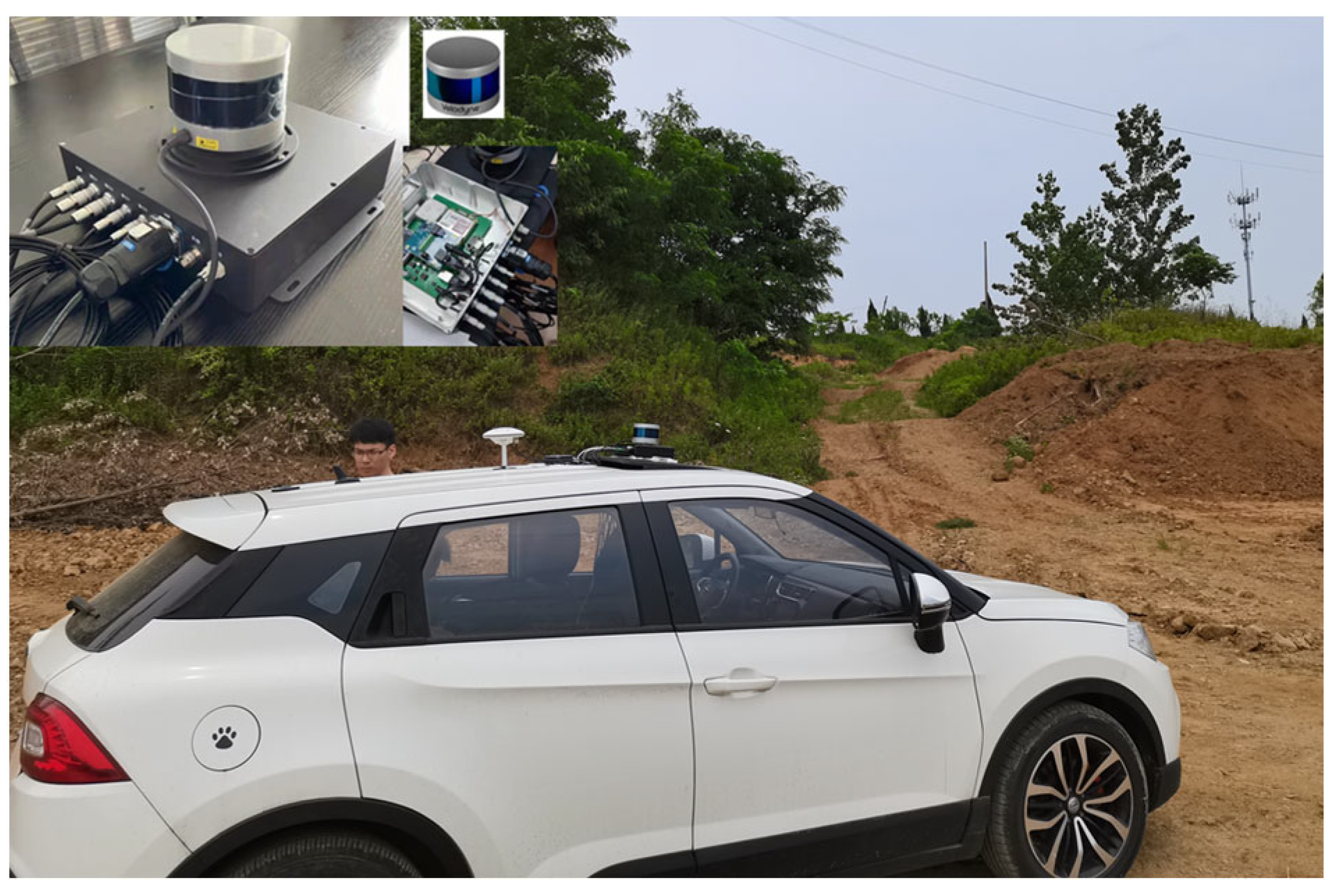
As shown in Figure 2, the vehicle platform incorporated a satellite navigation receiver, a 6-axis MEMS inertial navigation system and a 16-thread mechanical LiDAR. The LiDAR scanning frequency was 10 Hz, while the IMU output frequency was 100 Hz. The 1PPS signal from the satellite navigation receiver was synchronized with the UTC output time and its frequency was doubled to 10 Hz and 100 Hz, respectively, providing time synchronization services for the LiDAR and IMU and ensuring temporal alignment among the three sensors. Data processing was carried out using a small computer equipped with a 4-core Intel i7-8gen CPU.

2.3. Unified Coordinate System

First, transfer the IMU coordinate system to the LiDAR coordinate system, and then convert the GNSS/IMU combined absolute positioning results from WGS84 coordinate system (latitude, longitude, elevation) to the UTM (Universal Transverse Mercator) grid coordinate system. Finally, the GNSS results are transferred to the world coordinate system by fusing the original IMU with the extended Kalman filter estimator.

3. Fusion Methods

3.1. GNSS/INS Factor

GNSS raw observations can be utilized to obtain latitude, longitude, and elevation via RTK. GNSS/INS integrated navigation methods exhibit complementary characteristics. Therefore, integrated navigation is essential in multi-source fusion systems in complex environments.
GNSS/INS loose coupling usually uses a Kalman filter to address the system’s nonlinearities. The primary error parameters of the inertial sensors are incorporated into the system state vector of the Kalman filter. The GNSS/INS integrated navigation is based on the INS error equation [25]:
δ r ˙ = ω e n × δ r + δ v δ v ˙ = ( ω i e ω i n ) × δ v δ ψ × f + δ ψ ˙ = ω i n × δ ψ + ε = u , ε = u ε
δ r , δ v and δ ψ denote the position, velocity, and orientation error vectors, respectively. ω e n represents the rotation angular velocity vector of the navigation coordinate system with respect to the earth coordinate system. ω i e is the rotation angular velocity vector of the Earth coordinate system with respect to the inertial coordinate system. ω i n represents the rotation angular velocity vector of the navigation coordinate system with respect to the inertial coordinate system. f denotes the specific force vector measured by the accelerometer. and ε denote the acceleration random error vector and the gyro random error vector. u , u ε denotes white Gaussian noise.
For the velocity v g and position r g of the GNSS motion state at time t, the vector of the combined system is expressed as the difference between the velocity and position of IMU and GNSS. v i and r i are based on the mechanical arrangement of the IMU acceleration and angular rate:
z = v g v i , r g r i
The covariance matrix is constructed as follows:
P k = v v v r r v r r
The extended Kalman filter [26] is used to obtain the positioning results from loosely integrated navigation data fusion.

3.2. LIO Factor

3.2.1. Distortion Correction

The LIO factor is based on the improved LIO_SAM algorithm [19]. The low scanning frequency of LiDAR necessitates consideration of the impact of the vehicle platform’s speed on data acquisition. By leveraging the high-precision and short-term advantages of the IMU, motion compensation for scanning is performed, and a short-time approximate uniform-motion compensation model is established.
X i t = q X ^ i t + τ i τ t τ τ t r t
Here, τ , τ i , τ t represents a complete scanning period, scanning point time, and starting scanning time, respectively, and the point motion state matrix X ^ i t is the estimated value of X i t . The initial frame of lidar odometry is initialized using the rotation and translation obtained from IMU pre-integration [27]. The initial reference value for the subsequent frame is determined by adding the pose optimized through system fusion to the incremental rotation and translation obtained from IMU pre-integration at the current time.
The velocity v t + Δ t , position r t + Δ t , and rotation q t + Δ t state estimation models are calculated based on IMU measurements.
v t + Δ t = v t + g Δ t + q t W B a t b t a n t a Δ t r t + Δ t = r t + v t Δ t + 1 2 g Δ t 2 + 1 2 q t W B a t b t a n t a Δ t 2 q t + Δ t = q t exp ω t b t ω n t ω Δ t
Here, a t , ω t is the acceleration and angular velocity measurements at time t , respectively. b t a , n t a is the measurement deviation of acceleration measurement and random white noise. b t ω , n t ω is the measurement deviation of angular velocity and random white noise. g is the acceleration of gravity in the world coordinate system W . q t W B is the rotation of the inertial body coordinate system to the world coordinate system.

3.2.2. Feature Extraction

The different types of features in a 3D point cloud are distinguished by calculating the curvature threshold c t h , thereby extracting edge points and planar point features [15]. Points with curvature values greater than the threshold are classified as edge features, while those with curvature values less than the threshold are categorized as planar features.
The odometer identifies the corresponding feature of the current feature set F e t ,   F p t within the feature set F e t 1 ,   F p t 1 of the previous scan and estimates the sensor motion by conducting continuous scan matching for point-to-edge and point-to-plane features. Let d e , d p represent the distances from the point to the edge feature and from the point to the plane feature, respectively.

3.2.3. LiDAR Odometer

Using the 6-DoF representation, the Euler angles are transformed into a rotation matrix, and the Rodriguez formula is applied to perform the transformation.
R = e ω ^ θ = I + ω ^ sin θ + ω ^ 2 1 cos θ
Here, θ = r o l l , p i t c h , y a w , ω = T T , T = x , y , z .
Formulas for point-to-edge and point-to-plane constraints are derived, and the nonlinear Levenberg-Marquardt algorithm [28] is employed to solve the resulting equations.
f e θ , T = d e , f p θ , T = d p

3.3. Quality Control

3.3.1. GNSS/INS Quality Control

The latitude, longitude, and elevation of GNSS measurements are obtained via RTK. However, maintaining a fixed solution for these measurements can be challenging due to the influence of sheltered environments such as terrain and trees. It is essential to evaluate the availability of GNSS measurements using a multi-system GPS/BDS signal solution monitoring system. Fortunately, most receivers are equipped with signal solution state monitoring capabilities, which can provide feedback on the GNSS analysis state to the fusion system as a prior quality control strategy. The possible solution states include the following: (1) NONE; (2) SINGLE; (3) NARROW_FLOAT; (4) NARROW_INT. Generally, the ideal solution is NARROW_INT, which can either participate in the fusion solution or be directly utilized as the final localization result. However, even if integer ambiguities remain unresolved and the positioning result corresponds to a floating-point solution (e.g., NARROW_FLOAT), it can still participate in the fusion positioning process. This paper involves utilizing the covariance of GNSS/INS integrated navigation solutions as a prior probability judgment for GNSS/INS factors.

3.3.2. LIO Quality Control

It is assumed that features are repeatable in the scene and show a small change in the number of features between adjacent frames. This paper newly proposes the difference and approximate derivative variability of features and the standard deviation variability of features to characterize the repeatability of features in the scene, which is used as the prior discrimination of the availability of LIO.
Edge points and plane points have been found to perform well in a variety of settings, including schools and parks. However, the resolution of LiDAR is inherently limited. During high-speed motion, the actual sparsity of plane points derived from adjacent feature points can vary significantly. For example, in environments with few features, such as tunnels, the number of effective feature points decreases substantially. This can directly compromise odometry accuracy due to feature mismatching. To address this issue, the current frame is discarded if the number of extracted feature points falls below a predefined threshold, thus preventing degradation. To maintain system stability, the weight assigned to keyframes at a high risk of degradation should be reduced. Furthermore, a measure of uncertainty is introduced for matching feature value errors, in order to assess the associated risk of inaccurate feature matching during the fusion process.
The standard deviation variability of differences of features: σ d i f f :
n f e a t u r e A , e p o c h = c a r d ( A ) d i f f f e a t u r e i = n f e a t u r e i n f e a t u r e i 1 σ d i f f = s t d ( d i f f )
The standard deviation variability of features, σ A , n f e a t u r e i , represents the number of features at epoch i , and n f e a t u r e i equals 6 in the experiment of Section 4 below:
σ A = s t d ( A ) / n f e a t u r e i , n f e a t u r e A , e p o c h = c a r d ( A )

3.4. Fusion

3.4.1. Factor Graph Optimization

Factor graph optimization is well-suited to large-scale problems with sparse structures in real-world complex environments [29,30,31]. The Huber kernel function is used to address potential outliers in the input data of the least squares problem that may be caused by incorrect measurements. Using the loss function effectively mitigates the influence of these outliers on the optimization process. Specifically, the LossFunction minimizes the impact of large residuals on the final optimization result by reducing the weight assigned to them. The Schur complement method is utilized for the resolution of the optimization problem. In this approach, the block diagonal part of the Hessian matrix is computed using the sparse Cholesky decomposition method, while the remaining parts are handled using the dense QR decomposition method.
The residuals of the odometer in LIO are formulated as the errors in the rotation matrix R i j and translation vector t i j of adjacent frame motions. Specifically, the rotation matrix is represented as a quaternion, while the translation vector corresponds to positional displacements.
Δ l = min x i j 1 2 i ρ i f R i j , t i j 2
f R i j , t i j = q i   x j , q i   y j , q i   z j , q i   w j , t i   x j , t i   y j , t i   z j
The residuals of GNSS/INS are formulated as the positional errors in the northeast-down direction between adjacent frames within the UTM coordinate system. The integrated navigation result from GNSS/INS is utilized as the absolute position factor.
χ g k = X g 1 , X g 1 , , X g k
X g k = x g k , y g k , z g k

3.4.2. Inverse Weight of Uncertainty

In response to the divergent performance of satellite navigation and LiDAR sensors across a range of environments, sensor weights are dynamically adjusted by defining the prior factor for the newly proposed uncertainty measurement. For the GNSS/INS factor, the covariance matrix r r follows a Gaussian distribution and can therefore serve as the prior factor for uncertainty measurement in Gaussian error modeling. Position r g is the GNSS motion state, and position r I is calculated based on IMU measurements. The details are in Section 3.1.
ξ G N S S / I N S = r r = d i a g ε x g , ε y g , ε z g
r r = C o v ( r g , r I )
In order to prevent degradation and collapse resulting from feature repetition and sparsity, forced constraints on the inverse weight of the uncertainty metric are applied for LIO. When the LIO (LiDAR-Inertial Odometry) is operational, the uncertainty measurement corresponds to the standard deviation of the current static environment. If this value exceeds the predefined threshold Q σ d i f f and Q σ A , the uncertainty measure approaches infinity. The value of Q σ d i f f is 30 and Q σ A is 1.0%, respectively, in the experiment of Section 4 below. Let equaling 10,000 represent infinity.
ξ L I O = s t d ( T ) , σ d i f f Q σ d i f f &   σ A Q σ A , σ d i f f < Q σ d i f f σ A < Q σ A
T = x , y , z is the transition matrix of LIO in the current static environment. Q σ d i f f denotes the threshold of the standard deviation variability of differences of features σ d i f f . Q σ A denotes the threshold of the standard deviation variability of differences of features σ A . The reference threshold values were obtained by analyzing the results of feature repeatability in different environments, the details are in Section 5.

4. Experiments and Analysis

In order to verify the adaptability of the algorithm in complex environments, this study conducted positioning experiments in four representative scenarios: namely, tunnel, urban, campus, and mountainous environments. In the tunnel environment, the reliability and stability of the algorithm were assessed to evaluate the effectiveness of the quality control mechanism in scenarios characterized by sparse and repetitive features. The positioning accuracy of the algorithm was validated by comparison with existing multi-source fusion algorithms, such as FAST-LIO and LIO-SAM, between urban and campus scenes. In the mountainous environment, the continuity and robustness of the algorithm under complex conditions were examined. Concurrently, an analysis was conducted of the sparsity and repeatability of features extracted from lidar data across diverse scenarios. Furthermore, an assessment was undertaken of the impact of the quality control algorithm on sensor performance in varying environmental conditions.

4.1. Tunnel Environment Experiment

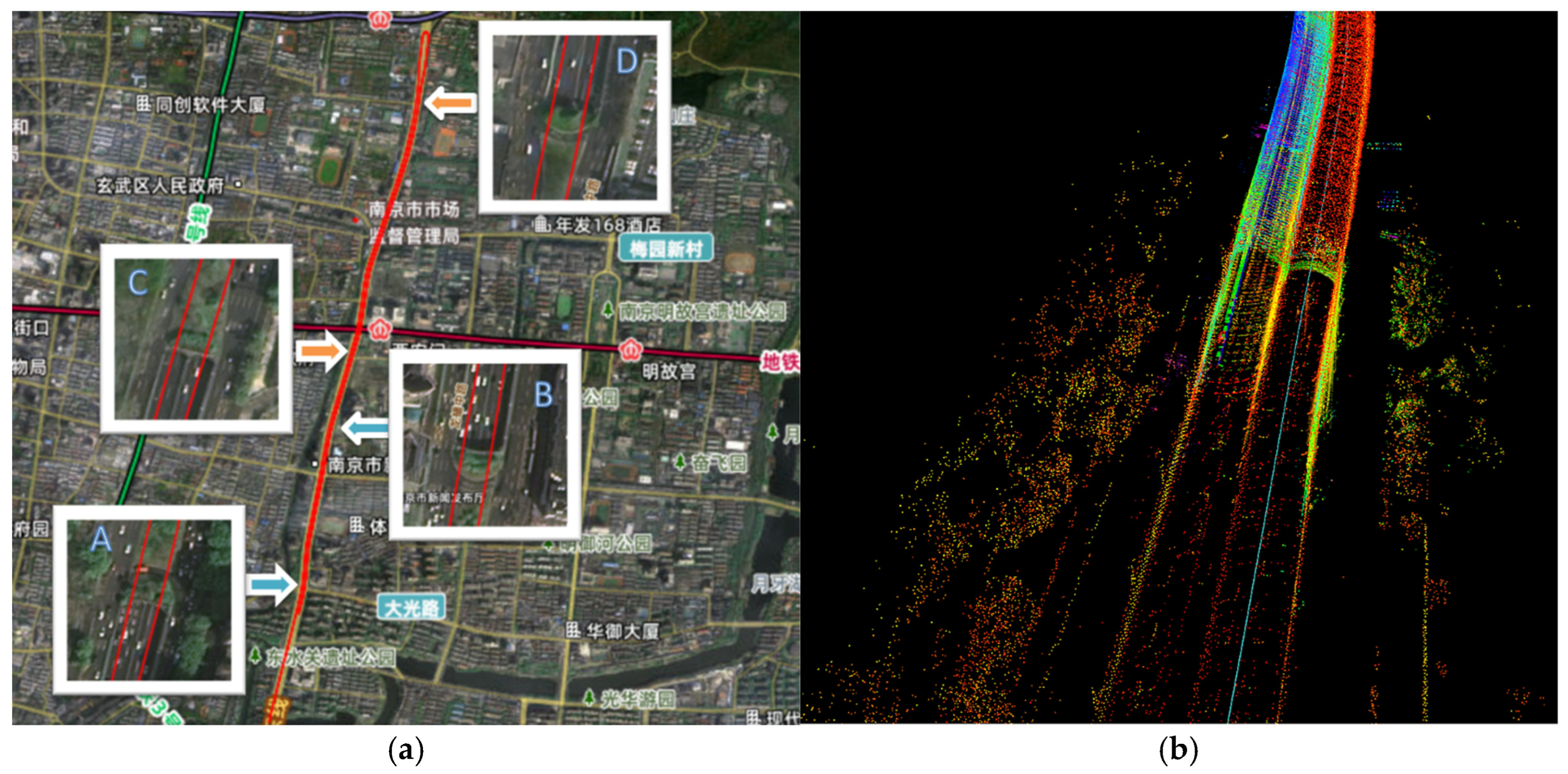
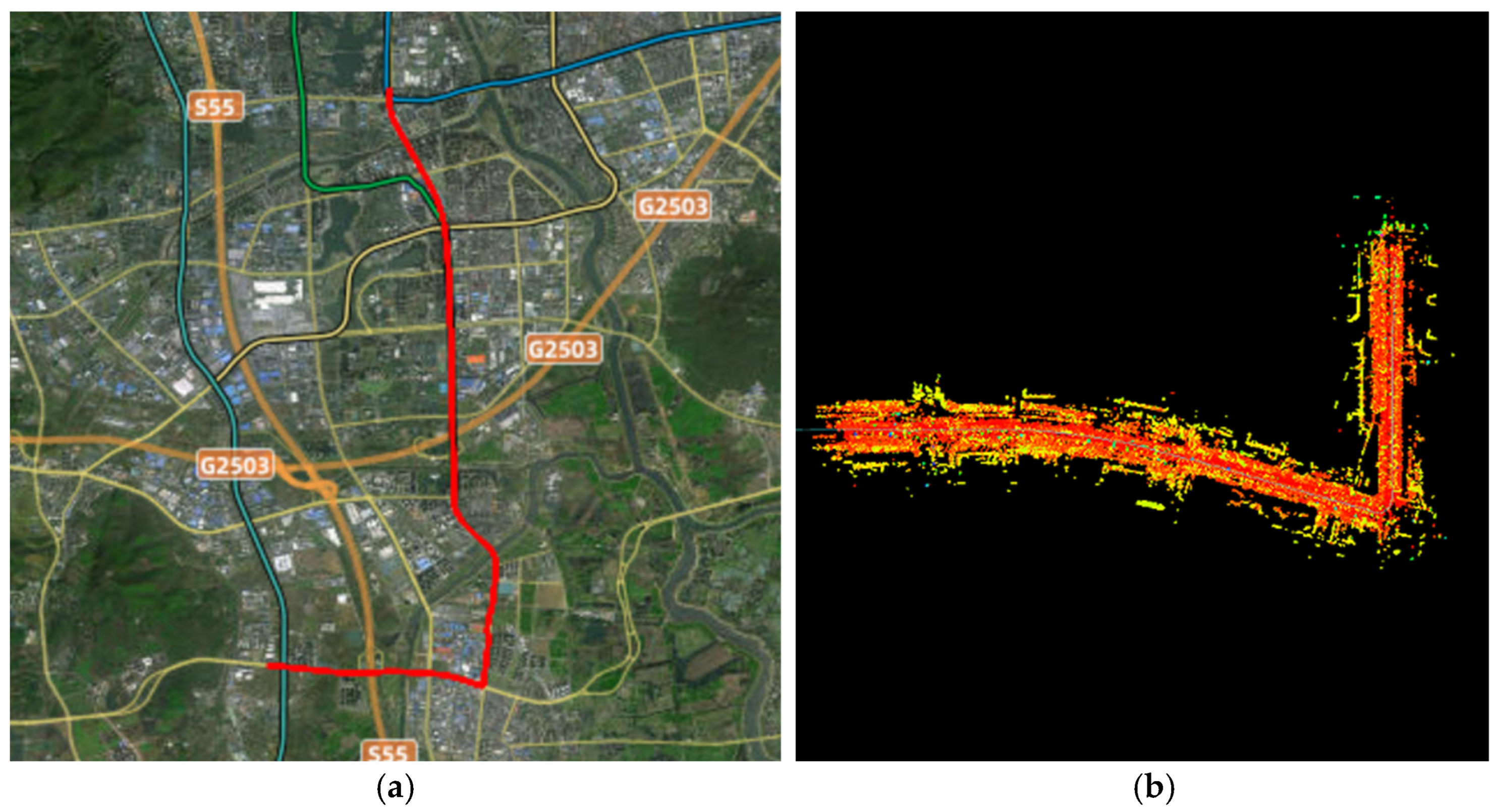
Initially, an experiment was conducted to ascertain the positioning of the tunnel environment. The vehicle successfully traversed the Tongjimen Tunnel (see Figure 3a(A,B), 1.0 km) and the Xi’anmen Tunnel (see Figure 3a(C,D), 1.84 km) at an average effective speed in excess of 40 km/h. The entire test section extended for approximately 8 km, with a total testing duration of 10 min. The positioning trajectory is illustrated in the figure. The findings demonstrate that the algorithm maintains continuous and smooth positioning in real time as the vehicle navigates through complex urban road conditions, including when entering and exiting tunnels.
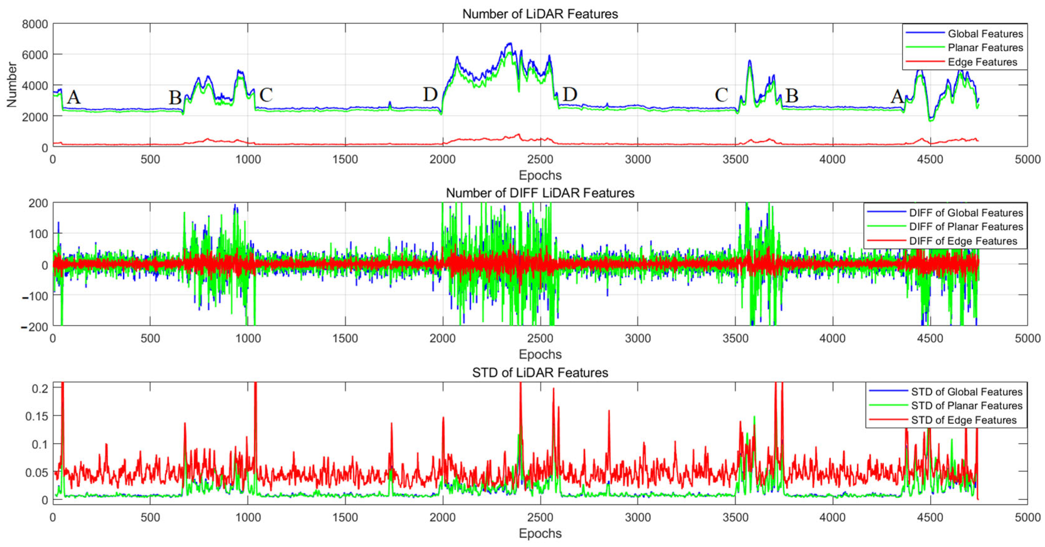
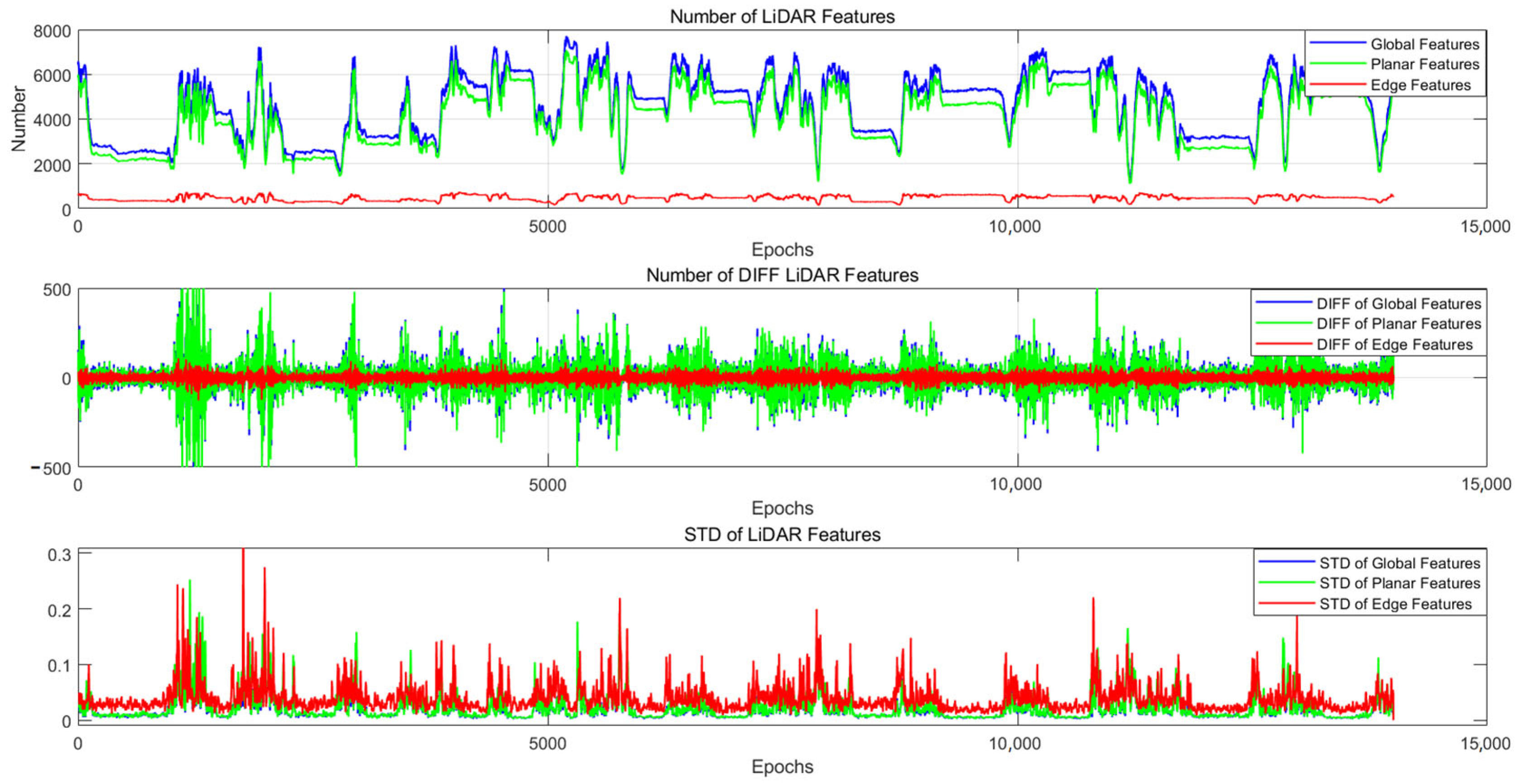
As demonstrated in Figure 4, within the primary section of the inner ring road, the number of LiDAR edge and planar feature points is comparatively elevated, and the distribution of the variation in the number of feature points between successive scanning frames is discernible. The standard deviation variability of differences of planar feature σ d i f f p is more than 90, and the standard deviation variability of planar feature’s σ A p average feature fluctuation rate is higher than 3.06%. The edge feature σ d i f f e is more than 90, and the σ A e average feature fluctuation rate is 5.11%. The average characteristic variability σ A is about 2.86%; this indicates that the feature repeatability is relatively low. Conversely, in the tunnel scenario, the number of LiDAR edge and planar feature points decreases, while the distribution of the standard deviation variability of differences of feature points remains relatively stable, suggesting that the scanning frame features exhibit a degree of repetitiveness. The standard deviation variability of differences of global tunnel feature σ d i f f is 23.73, the standard deviation variability of global tunnel feature σ A is about 0.79%, the planar feature σ d i f f p is 21.73, and the planar feature variability σ A p is 0.78%.
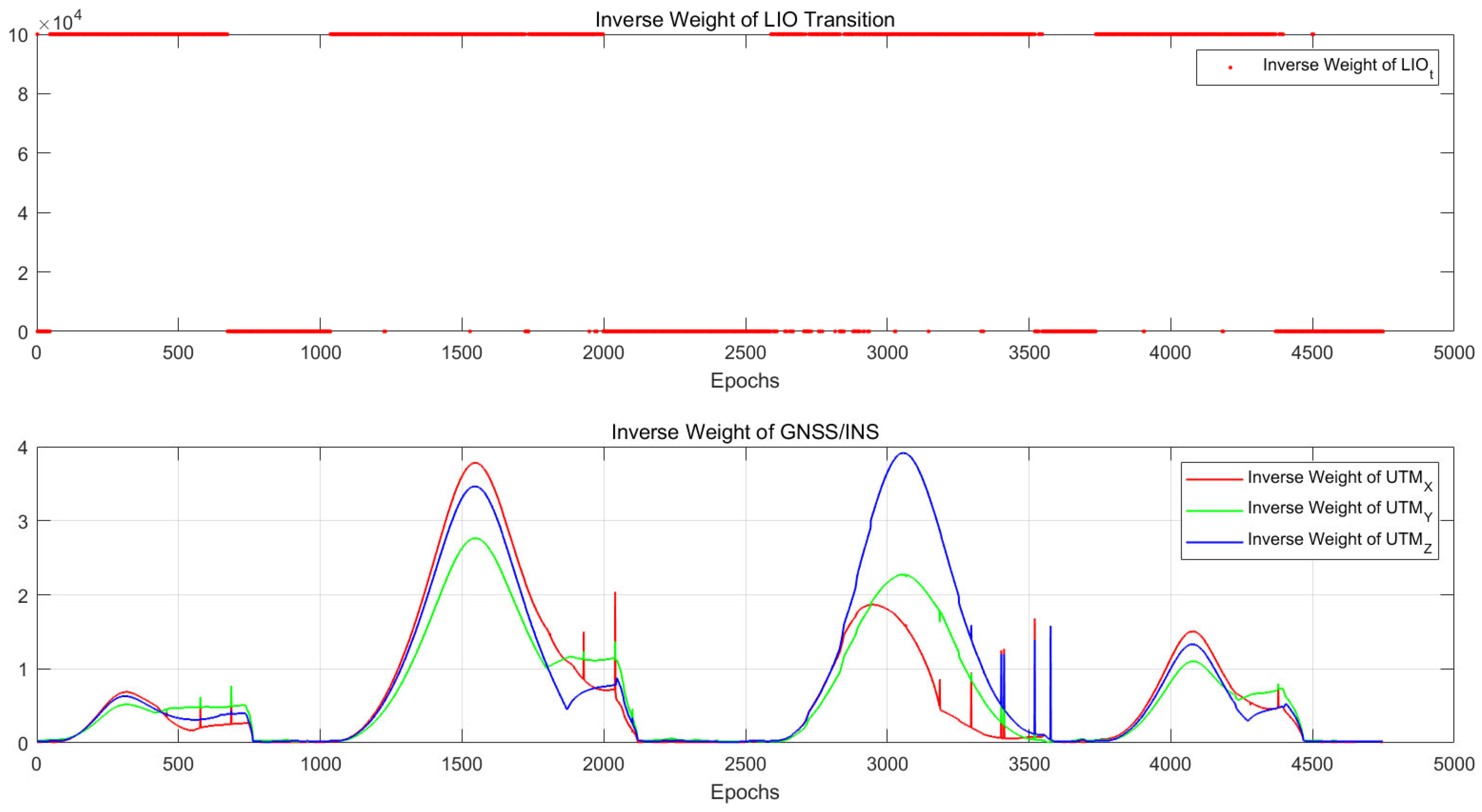
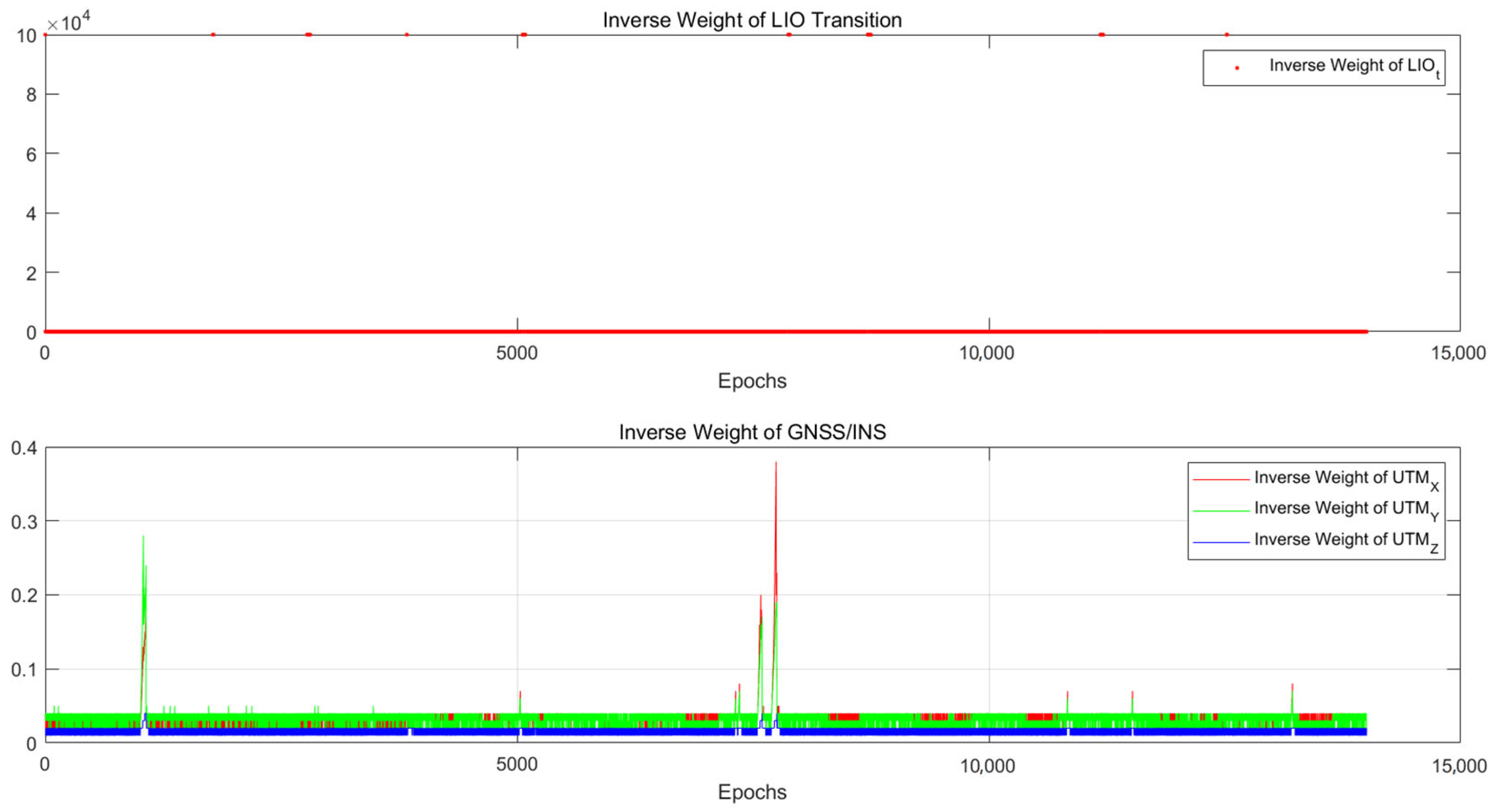
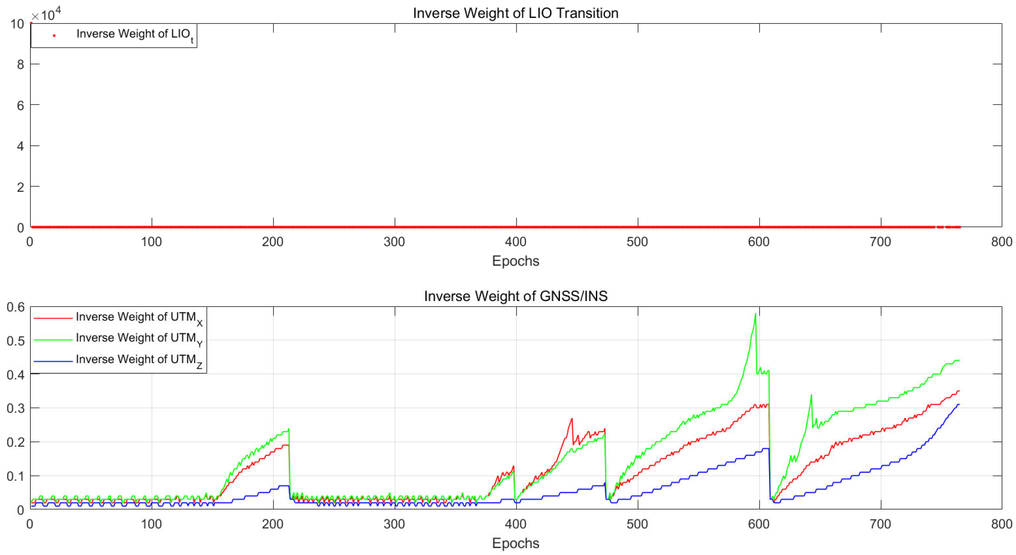
The value is significantly lower than that of the urban road segment, with higher feature repeatability and lower availability of LIO. Consequently, the corresponding inverse weight is increased or even becomes unavailable. When the vehicle traverses complex urban road conditions and tunnels, the weights of LIO and GNSS/INS positioning are specifically adjusted. The inverse weight serves as the prior Gaussian noise input value. As illustrated in Figure 5, under urban road conditions visible to navigation satellites, the inverse weight of GNSS/INS integrated navigation remains at a relatively low level, with an average value not exceeding 0.1. In the tunnel, the LIO maintains a relatively high inverse weight to avoid degradation and negative positioning performance.

4.2. Urban Environment Experiment

The vehicle traversed urban roads, traffic intersections, billboards, and viaducts at an average effective speed exceeding 40 km/h in Nanjing City, covering a total distance of approximately 15 km over a test duration of 30 min. The positioning trajectory is illustrated in Figure 6. The results indicate that the algorithm maintains continuous and smooth real-time positioning even after traversing complex urban road conditions, including viaducts, with a positioning accuracy (RMSE) better than 0.18 m.
As illustrated in Figure 7 and Figure 8, the number of LiDAR edge and planar feature points is comparatively high in an urban environment, and the distribution of the difference in the number of feature points between scanning frames exhibits significant variation. The planar feature σ d i f f p is close to 80, the average characteristic variability of σ A p is higher than 2.23%, the edge feature σ d i f f e is more than 20, and the average characteristic variability of σ A e is 3.92%. The average characteristic variability of σ A is about 2.10%. The findings indicate that the reproducibility of features is diminished, the accessibility of LIO is augmented, and the associated inverse weight is diminished.

4.3. Campus Environment Experiment

The vehicle traversed the campus road, which was closed to traffic, at an average effective speed of approximately 17 km/h, covering a total distance of about 0.85 km in 3 min. The positioning trajectory is illustrated in the Figure 9. The results indicate that the algorithm maintains continuous and smooth real-time positioning even after the vehicle passes through campus road conditions, with a positioning accuracy (RMSE) better than 0.23 m.
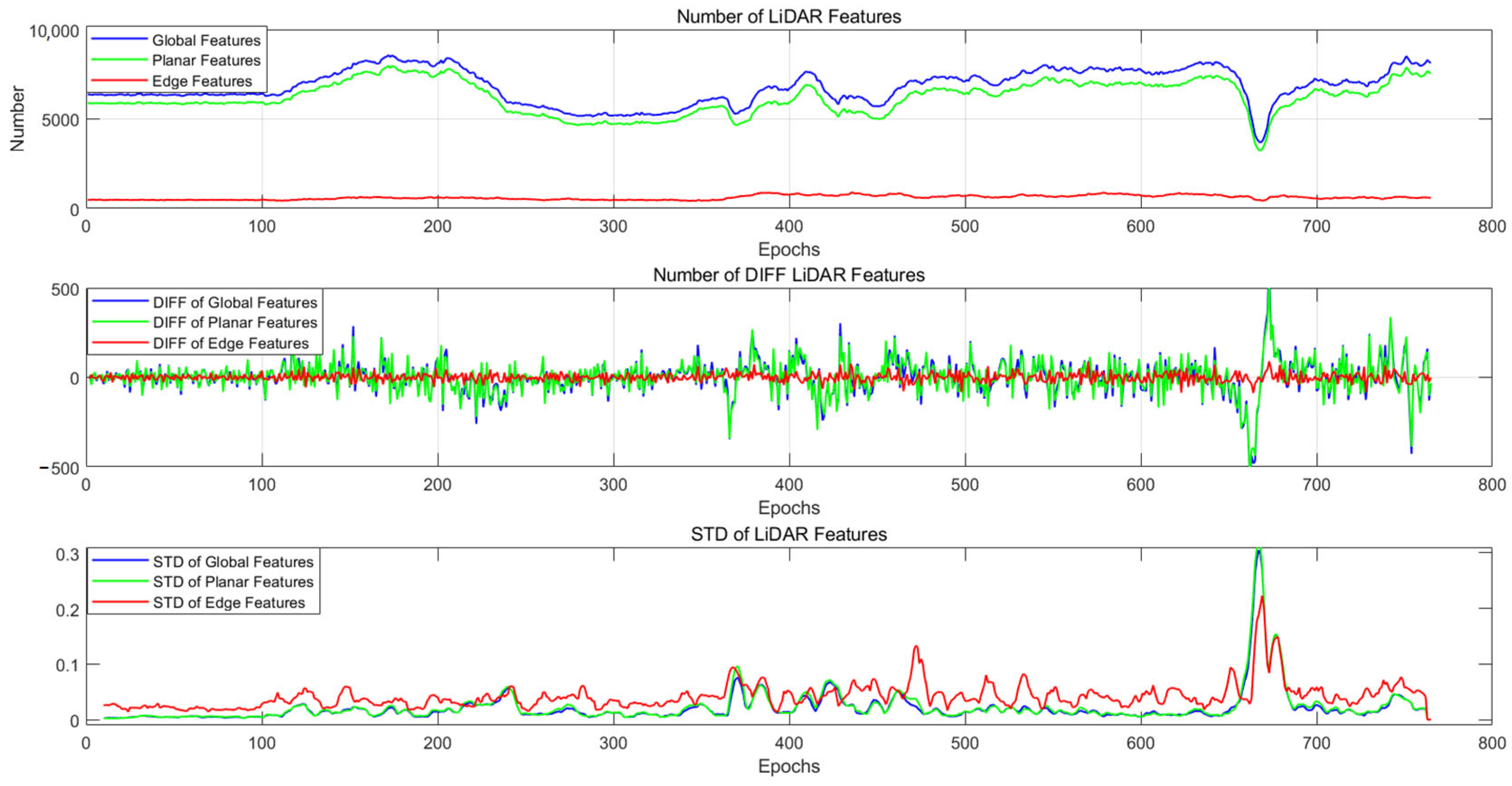
As illustrated in Figure 10 and Figure 11, the campus road section features a rigid and regular building structure. The number of LiDAR edge and planar feature points is relatively high, and the distribution of the difference in the number of scanning frame feature points shows significant variation. Specifically, the planar feature σ d i f f p exceeds 90, with an average characteristic variability of σ A p higher than 2.28%. The edge feature σ d i f f e exceeds 25, with an average characteristic variability of σ A e at 4.16%. The overall average characteristic variability of σ A is approximately 2.14%. These findings indicate a reduction in feature repeatability, increased availability of LIO, and a corresponding decrease in inverse weighting. Furthermore, the positioning accuracy of GNSS/INS integrated navigation diverges in road sections covered by buildings, accompanied by a synchronous increase in inverse weighting.

4.4. Mountain Environment Experiment

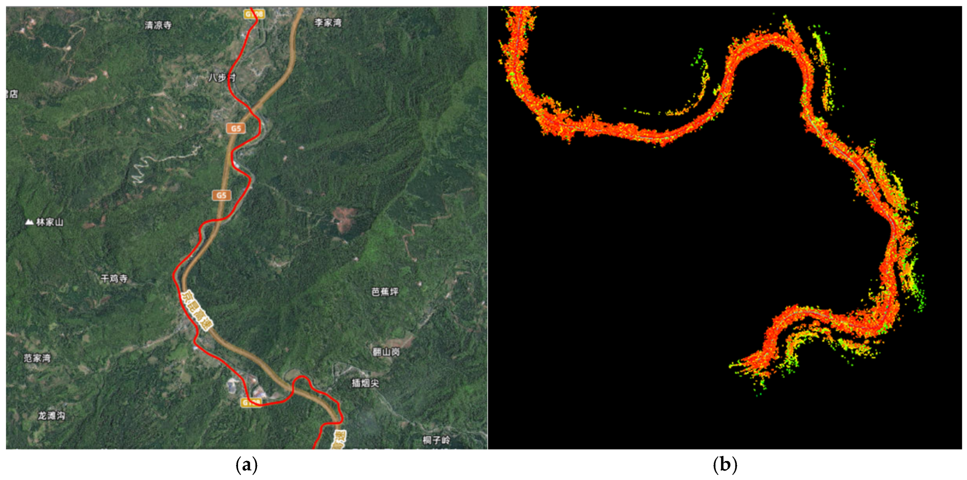
The vehicle finally proceeded along a winding mountain road at an average effective speed of approximately 40 km/h. The total distance covered was about 8.5 km, with the journey taking 12 min. The positioning trajectory is illustrated in Figure 12. The results indicate that the algorithm can maintain continuous and smooth positioning in real time even when the vehicle passes through complex mountainous terrain and is impeded by mountains. The positioning accuracy (RMSE) is better than 0.21 m.
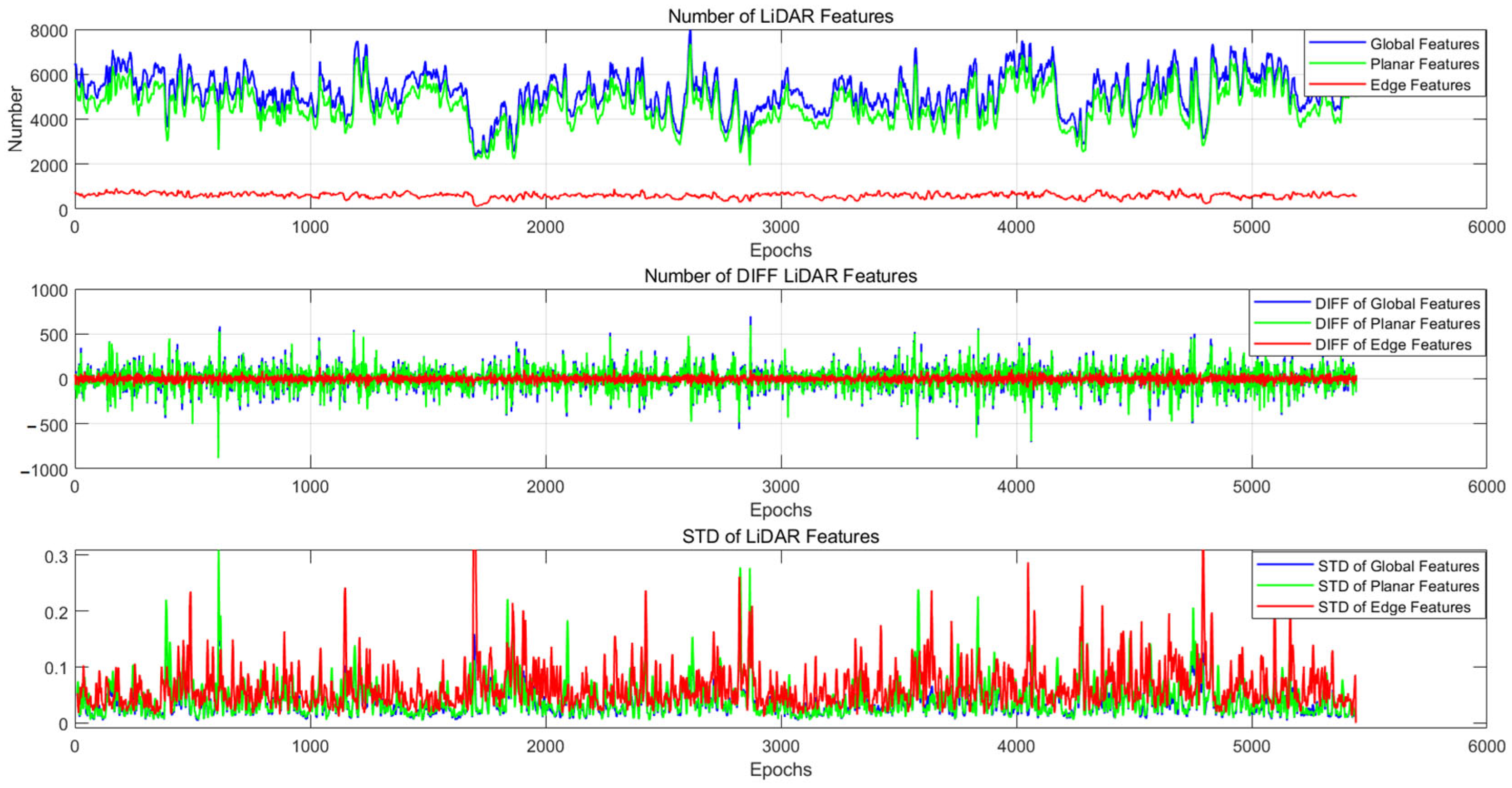
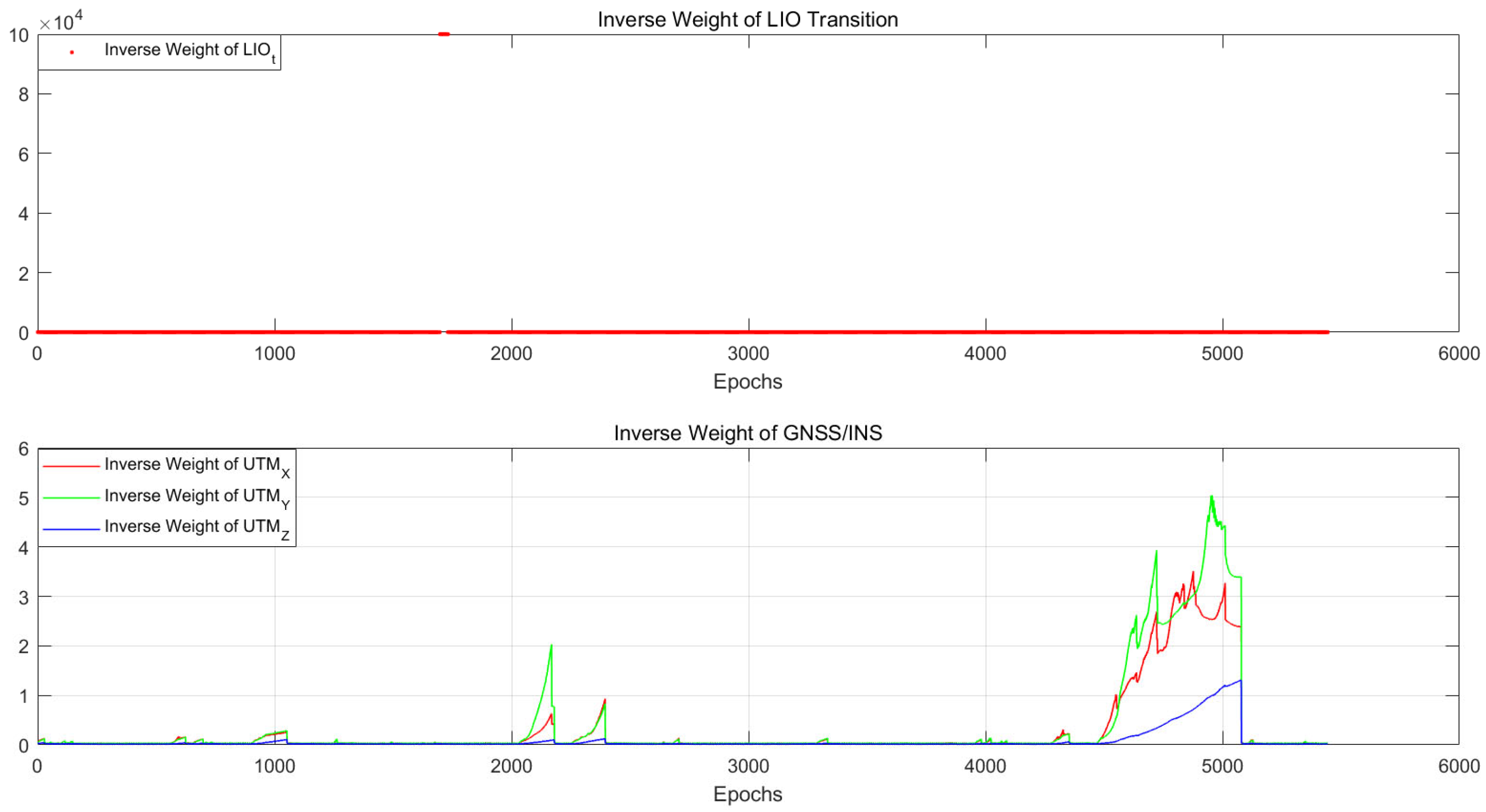
As illustrated in Figure 13 and Figure 14, within a mountainous environment, the environmental structure exhibits rigidity. The number of LiDAR edge and planar feature points is relatively high, and the distribution of differences in the number of scanning frame feature points is notably distinct. Specifically, the planar feature count σ d i f f p exceeds 110, with an average standard deviation fluctuation rate exceeding 4.20%. The edge feature count σ d i f f e is approximately 30, accompanied by an average standard deviation variability of 6.43%. The overall average characteristic variability of σ A is approximately 3.95%. These observations indicate a reduction in feature repeatability. However, the availability of LIO remains high, with the corresponding inverse weight being consistently low. In contrast, for some mountainous roads sheltered from GNSS signals, the positioning accuracy of the GNSS/INS integrated navigation system diverges, while the inverse weight increases synchronously.

4.5. Accuracy of Positioning and Mapping

As demonstrated in Table 1, the present article undertakes a comparative analysis of the algorithm in question with regard to its positioning accuracy, reliability, and robustness. This is undertaken against the backdrop of state-of-the-art algorithms, including LIO_SAM, FAST_LIO, and LEGO_LOAM. Comparative studies have been designed between scenarios with the quality-control module (OURS) and without the quality-control module (LIO_SAM or LIO_SAM (gps)), because the framework of this paper is based on the improved LIO_SAM algorithm. Firstly, with regard to reliability and robustness, the algorithm in question was demonstrated to display versatility in four distinct real-world environments, namely tunnel, urban, campus, and mountainous settings. It has been observed to exhibit robust performance, characterised by integrity and smoothness, in the aforementioned environments. In contrast, other algorithms have proven to be incapable of completing large-scale scene positioning tests, due to the presence of large-scale drifting and system degradation, with the exception of the campus environment. Compared with the LIO_SAM algorithm, our algorithm improves the robust running time by 44% in terms of availability in large-scale urban (2014s) tests. In addition, the algorithm exhibits superior positioning accuracy compared to other methods, achieving a positioning accuracy (RMSE) of 0.18 and 0.21 m in large-scale, long-duration urban and mountainous settings, respectively. Although adding GPS factors to the LIO_SAM algorithm can improve positioning accuracy in some small-scale scenarios, it can also increase the risk of system degradation caused by forced constraints.
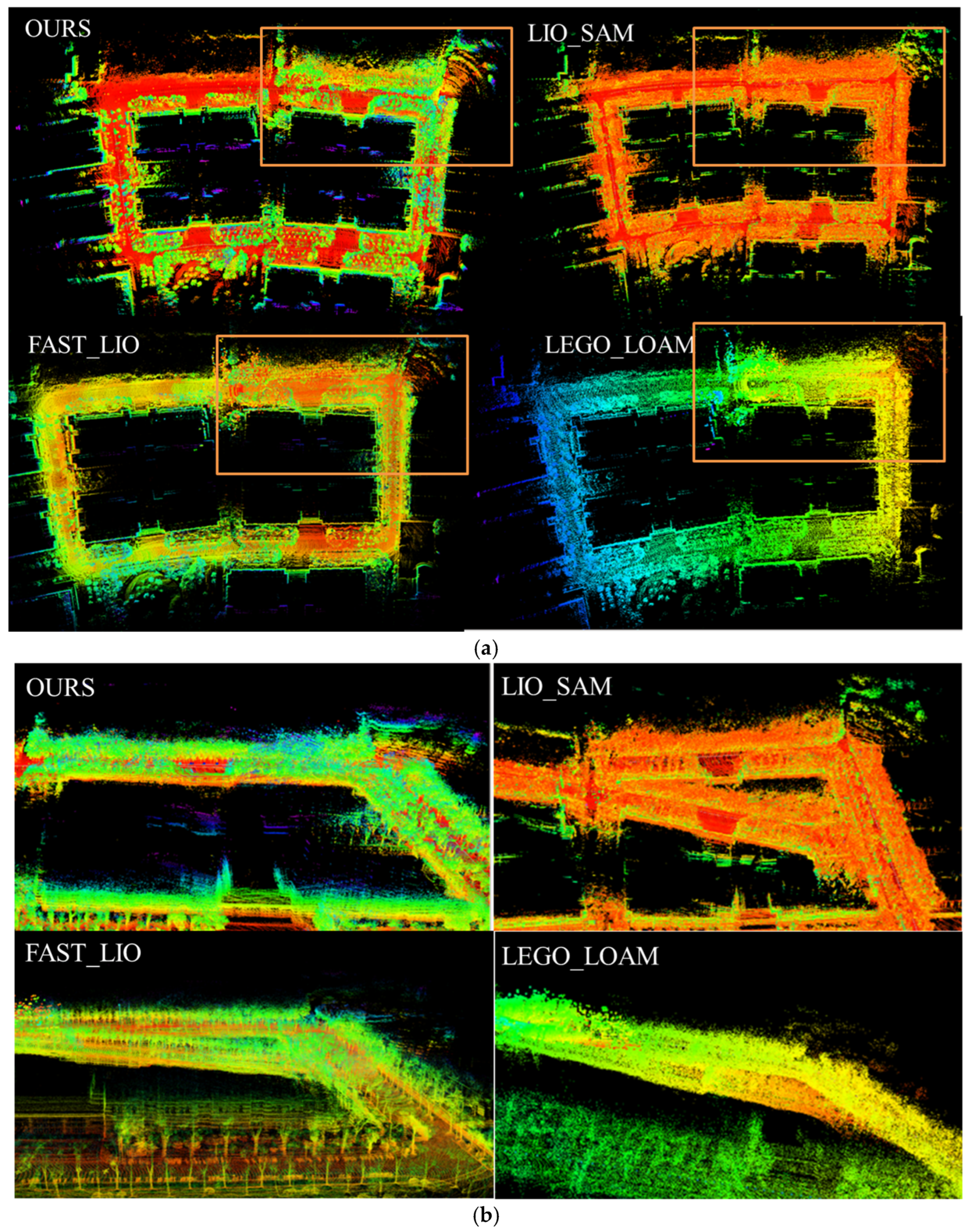
As illustrated in Figure 15, with regard to the accuracy of mapping in a closed-loop campus environment, while all the comparison algorithms attain horizontal closure of real-time mapping upon returning to the initial point, there are evident mapping errors in the vertical direction. The algorithm presented in this article demonstrates a superior capacity for convergence in the elevation direction when compared to alternative algorithms.

5. Discussion

The repeatability of point cloud features is an important cause of LIO system degradation due to the inability to correctly estimate the position and orientation in the environment. Should repetitive features be correctly extracted, the methods will demonstrate their application potential in real, complex environments. The quality control strategy can be divided into two aspects: front-end and back-end. The front end of the system is primarily responsible for feature extraction or sensor status monitoring. The primary focus of back-end optimization is the fusion method and weight distribution strategies employed. In this paper, we calculate the difference and approximate derivative variability and the standard deviation variability derived from LiDAR point clouds across four real environments: tunnel, urban, campus, and mountainous environments. These calculations aim to monitor the repeatability of features within every scene and serve as a prior indicator for assessing the availability of LIO.
As shown in Table 2, the mechanical LiDAR data exhibit high repeatability in tunnel environments, with significantly lower feature variability compared to other environments such as urban and campus ones, so there are differences in the availability of LiDAR sensors in different environments. In tunnel environments, the planar feature variability is less than 22, the edge feature variability is below 10, and the average standard deviation percentage of the planar feature is less than 0.8%. Conversely, in mountainous environments, the repeatability of lidar features is relatively low and the planar feature count exceeds 110, with an average standard deviation variability exceeding 4.20%. The edge feature count is approximately 30, accompanied by an average standard deviation variability of 6.43%.
A comprehensive analysis of positioning accuracy and availability is presented in Table 1, while feature repeatability statistics are presented in Table 2. The weight of the LIO must be carefully adjusted if the reference threshold values Q σ d i f f and Q σ A are used as constraints to reduce the risk of degradation by less than 30 and 1.0%, respectively. The purpose of weight adjustment is to prevent the multi-source fusion system from failing due to large-scale offsets and LIO degradation. Furthermore, the absence of weight adjustment across varying environments renders the tunnel environment susceptible to system degradation, attributable to the reproducibility of lidar features and the paucity of point clouds. In order to ensure effective quality control of the system, it is necessary to adjust the weights with stringent constraints. In contrast, in large-scale, long-duration environments such as urban and mountain canyons, lidar point cloud features exhibit significant fluctuations. This enables the utilization and complementary capabilities of LIO. Although GNSS factors can improve positioning accuracy in certain small-scale scenarios, they also increase the risk of system degradation resulting from forced constraints, such as LIO_SAM (gps). Satellite navigation systems are prone to divergence due to multipath effects. In such scenarios, real-time weight adjustment is essential to ensure reliability and robustness.

6. Conclusions

Despite the advancement of multi-source fusion positioning frameworks in enhancing positioning accuracy, the reliability and robustness of multi-source fusion positioning algorithms remain substantial challenges in real, complex environments. These include system degradation in feature repetition scenarios and sudden forcing false absolute localization constraints. To address these challenges, this paper proposes the standard deviation variability of differences of features σ d i f f and the standard deviation variability of features σ A to evaluate the repeatability of LiDAR features in environments. In the back end, the Gaussian uncertainty measurement weights within the factor graph are dynamically updated in real time, allowing for adaptive adjustment of sensor fusion weights in different environments. In conclusion, sensor quality control plays a crucial role in ensuring reliability and robustness of multi-source fusion localization. It is evident that, despite the capacity of GNSS factors to enhance the precision of positioning in certain limited contexts, they concomitantly engender an escalation in the vulnerability of the system to degradation, a consequence of the imposition of constraints. The quality control of GNSS positioning is also of crucial importance in the context of multi-source fusion. The development of research methods for GNSS quality control is therefore paramount, with a view to enhancing the robustness of multi-source fusion localization. Potential approaches in this regard include GNSS state assessment and error suppression based on other sensors.

Author Contributions

Z.Z. conceived the idea and designed the experiments with C.S. and X.W., Z.Z. and C.S. wrote the main manuscript. S.P. and J.Z. reviewed the paper. B.Y. provided technical support. All components of this research study were carried out under the supervision of C.S. All authors have read and agreed to the published version of the manuscript.

Funding

This research was funded by the Science and Technology Innovation Program of Xiongan New Area (Grant No.2023XAGG0081) “A New-Generation Space-Ground Cooperative Integrated PNT Network and Its Application System in Xiongan”.

Data Availability Statement

Dataset Availability Statements are available in the section “National Public Science and Technology Center for Basic Disciplines-2019YFC1511504” at https://www.nbsdc.cn/archive (accessed on 10 June 2023).

Acknowledgments

This work is also supported by the Hebei Province Strategic Technology Special Fund Project (no.23319902L), University Research Collaboration Project, the GNSS/LEO Integrated Cloud Processing Platform for rapid and High-Precision Positioning Services, SKX202010044.

Conflicts of Interest

The authors Ziteng Zhang, Chuanzhen Sheng, Xingxing Wang, Jingkui Zhang, and Baoguo Yu were employed by The 54th Research Institute of China Electronics Technology Group Corporation. The remaining authors declare that the research was conducted in the absence of any commercial or financial relationships that could be construed as a potential conflict of interest.

References

  1. Li, X.; Xu, Q.; Li, X.; Xin, H.; Yuan, Y.; Shen, Z.; Zhou, Y. Improving PPP-RTK-based vehicle navigation in urban environments via multilayer perceptron-based NLOS signal detection. GPS Solut. 2023, 28, 15. [Google Scholar] [CrossRef]
  2. Liu, H.; Zhang, Z.; Sheng, C.; Yu, B.; Gao, W.; Meng, X. Fast and Reliable Network RTK Positioning Based on Multi-Frequency Sequential Ambiguity Resolution under Significant Atmospheric Biases. Remote Sens. 2024, 16, 2320. [Google Scholar] [CrossRef]
  3. Kim, J.; Sukkarieh, S. 6DOF SLAM aided GNSS/INS navigation in GNSS denied and unknown environments. J. Glob. Position. Syst. 2005, 4, 120–128. [Google Scholar] [CrossRef]
  4. Li, L.; Nie, W.; Zong, W.; Xu, T.; Li, M.; Jiang, N.; Zhang, W. High-Precision Multi-Source Fusion Navigation Solutions for Complex and Dynamic Urban Environments. Remote. Sens. 2025, 17, 1371. [Google Scholar] [CrossRef]
  5. Xu, B.; Zhang, S.; Wang, J.; Li, J. An innovation-based cycle-slip, multipath estimation, detection and mitigation method for tightly coupled GNSS/INS/Vision navigation in urban areas. arXiv 2024, arXiv:2409.03433. [Google Scholar] [CrossRef]
  6. Qin, T.; Li, P.; Shen, S. VINS-Mono: A Robust and Versatile Monocular Visual-Inertial State Estimator. IEEE Trans. Robot. 2018, 34, 1004–1020. [Google Scholar] [CrossRef]
  7. Campos, C.; Elvira, R.; Rodriguez, J.J.G.; Montiel, J.M.M.; Tardos, J.D. ORB-SLAM3: An Accurate Open-Source Library for Visual, Visual-Inertial and Multi-Map SLAM. IEEE Trans. Robot. 2021, 37, 1874–1890. [Google Scholar] [CrossRef]
  8. Zhang, X.; Zhu, F.; Tao, X.; Duan, R. New optimal smoothing scheme for improving relative and absolute accuracy of tightly coupled GNSS/SINS integration. Gps Solut. 2017, 21, 861–872. [Google Scholar] [CrossRef]
  9. Yan, G.; Wang, J.; Zhou, X. High-Precision Simulator for Strapdown Inertial Navigation Systems Based on Real Dynamics from GNSS and IMU Integration. In Proceedings of the China Satellite Navigation Conference (CSNC), Xi’an, China, 13–15 May 2015; Springer: Berlin/Heidelberg, Germany, 2015. [Google Scholar] [CrossRef]
  10. Obst, M.; Bauer, S.; Reisdorf, P.; Wanielik, G. Multipath Detection with 3D Digital Maps for Robust Multi-Constellation GNSS/INS Vehicle Localization in Urban Areas. In Proceedings of the Intelligent Vehicles Symposium (IV), Madrid, Spain, 3–7 June 2012. [Google Scholar] [CrossRef]
  11. Kim, S.H.; Jho, C.W.; Hong, H.K. Automatic Registration Method for Multiple 3D Range Data Sets. J. KISS Softw. Appl. 2003, 30, 1239–1246. [Google Scholar]
  12. Dellenbach, P.; Deschaud, J.-E.; Jacquet, B.; Goulette, F. CT-ICP: Real-time Elastic LiDAR Odometry with Loop Closure. In Proceedings of the 2022 International Conference on Robotics and Automation (ICRA), Philadelphia, PA, USA, 23–27 May 2022. [Google Scholar] [CrossRef]
  13. Koide, K.; Miura, J.; Menegatti, E. A Portable 3D LIDAR-based System for Long-term and Wide-area People Behavior Measurement. Int. J. Adv. Robot. Syst. 2019, 16, 1729881419841532. [Google Scholar] [CrossRef]
  14. Koide, K.; Miura, J.; Menegatti, E. Hdl_Graph_Slam[EB/OL]. 2018. Available online: https://github.com/koide3/hdl_graph_slam (accessed on 5 December 2020).
  15. Zhang, J.; Singh, S. Low-drift and Real-time LiDAR Odometry and Mapping. Auton. Robot. 2017, 41, 401–416. [Google Scholar] [CrossRef]
  16. Wang, H.; Wang, C.; Chen, C.; Xie, L. F-LOAM: Fast LiDAR Odometry and Mapping. In Proceedings of the 2021 IEEE/RSJ International Conference on Intelligent Robots and Systems (IROS), Prague, Czech Republic, 27 September–1 October 2021; pp. 4390–4396. [Google Scholar]
  17. Shan, T.; Englot, B. Lego-loam: Lightweight and ground-optimized LiDAR odometry and mapping on variable terrain. In Proceedings of the 2018 IEEE/RSJ International Conference on Intelligent Robots and Systems (IROS), Madrid, Spain, 1–5 October 2018; pp. 4758–4765. [Google Scholar]
  18. Kaess, M.; Johannsson, H.; Roberts, R.; Ila, V.; Leonard, J.J.; Dellaert, F. iSAM2: Incremental smoothing and mapping using the Bayes tree. Int. J. Robot. Res. 2021, 31, 216–235. [Google Scholar] [CrossRef]
  19. Shan, T.; Englot, B.; Meyers, D.; Wang, W.; Ratti, C.; Rus, D. LIO-SAM: Tightly-coupled Lidar Inertial Odometry via Smoothing and Mapping. In Proceedings of the 2020 IEEE/RSJ International Conference on Intelligent Robots and Systems (IROS), Las Vegas, NV, USA, 24 October 2020–24 January 2021. [Google Scholar] [CrossRef]
  20. Xu, W.; Zhang, F. FAST-LIO: A Fast, Robust LiDAR-inertial Odometry Package by Tightly-Coupled Iterated Kalman Filter. IEEE Robot. Autom. Lett. 2021, 6, 3317–3324. [Google Scholar] [CrossRef]
  21. Xu, W.; Cai, Y.; He, D.; Lin, J.; Zhang, F. FAST-LIO2: Fast Direct LiDAR-Inertial Odometry. IEEE Trans. Robot. 2022, 38, 2053–2073. [Google Scholar] [CrossRef]
  22. Qin, C.; Ye, H.; Pranata, C.E.; Han, J.; Zhang, S.; Liu, M. LINS: A LiDAR-Inertial State Estimator for Robust and Efficient Navigation. In Proceedings of the 2020 IEEE International Conference on Robotics and Automation (ICRA), Paris, France, 31 May–31 August 2020; pp. 8899–8906. [Google Scholar]
  23. Shan, T.; Englot, B.; Ratti, C.; Rus, D. LVI-SAM: Tightly-coupled LiDAR-Visual-Inertial Odometry via Smoothing and Mapping. In Proceedings of the 2021 IEEE International Conference on Robotics and Automation (ICRA), Xi’an, China, 30 May–5 June 2021. [Google Scholar] [CrossRef]
  24. Zheng, C.; Zhu, Q.; Xu, W.; Liu, X.; Guo, Q.; Zhang, F. FAST-LIVO: Fast and Tightly-coupled Sparse-Direct LiDAR-Inertial-Visual Odometry. In Proceedings of the 2022 IEEE/RSJ International Conference on Intelligent Robots and Systems (IROS), Kyoto, Japan, 23–27 October 2022. [Google Scholar] [CrossRef]
  25. Titterton, D.; Weston, J. Strapdown Inertial Navigation Technology, 2nd ed.; IET: London, UK, 2005; Volume 20, pp. 33–34. [Google Scholar] [CrossRef]
  26. Niu, X.J.; Zhang, Q.; Gong, L.L.; Liu, C.; Zhang, H.; Shi, C.; Wang, J.; Coleman, M. Development and evaluation of GNSS/INS data processing software for position and orientation systems. Surv. Rev. 2014, 47, 87–98. [Google Scholar] [CrossRef]
  27. Forster, C.; Carlone, L.; Dellaert, F.; Scaramuzza, D. On-Manifold Preintegration for Real-Time Visual-Inertial Odometry. IEEE Trans. Robot. 2016, 33, 1–21. [Google Scholar] [CrossRef]
  28. Triggs, B.; McLauchlan, P.F.; Hartley, R.I.; Fitzgibbon, A.W. Bundle adjustment—A modern synthesis. In Proceedings of the International Workshop on Vision Algorithms, Corfu, Greece, 21–22 September 1999; Springer: Berlin/Heidelberg, Germany, 1999; pp. 298–372. [Google Scholar]
  29. Indelman, V.; Williams, S.; Kaess, M.; Dellaert, F. Information Fusion in Navigation Systems via Factor Graph Based Incremental Smoothing. Robot. Auton. Syst. 2013, 61, 721–738. [Google Scholar] [CrossRef]
  30. Agarwal, S.; Mierle, K. Ceres-Solver[EB/OL]. 2015. Available online: http://www.ceres-solver.org (accessed on 10 May 2022).
  31. Kaess, M.; Ranganathan, A.; Dellaert, F. iSAM: Incremental Smoothing and Mapping. IEEE Trans. Robot. 2008, 24, 1365–1378. [Google Scholar] [CrossRef]
  32. Sturm, J.; Engelhard, N.; Endres, F.; Burgard, W.; Cremers, D. A benchmark for the evaluation of RGB-D SLAM systems. In Proceedings of the 2012 IEEE/RSJ International Conference on Intelligent Robots and Systems, Vilamoura-Algarve, Portugal, 7–12 October 2012. [Google Scholar] [CrossRef]
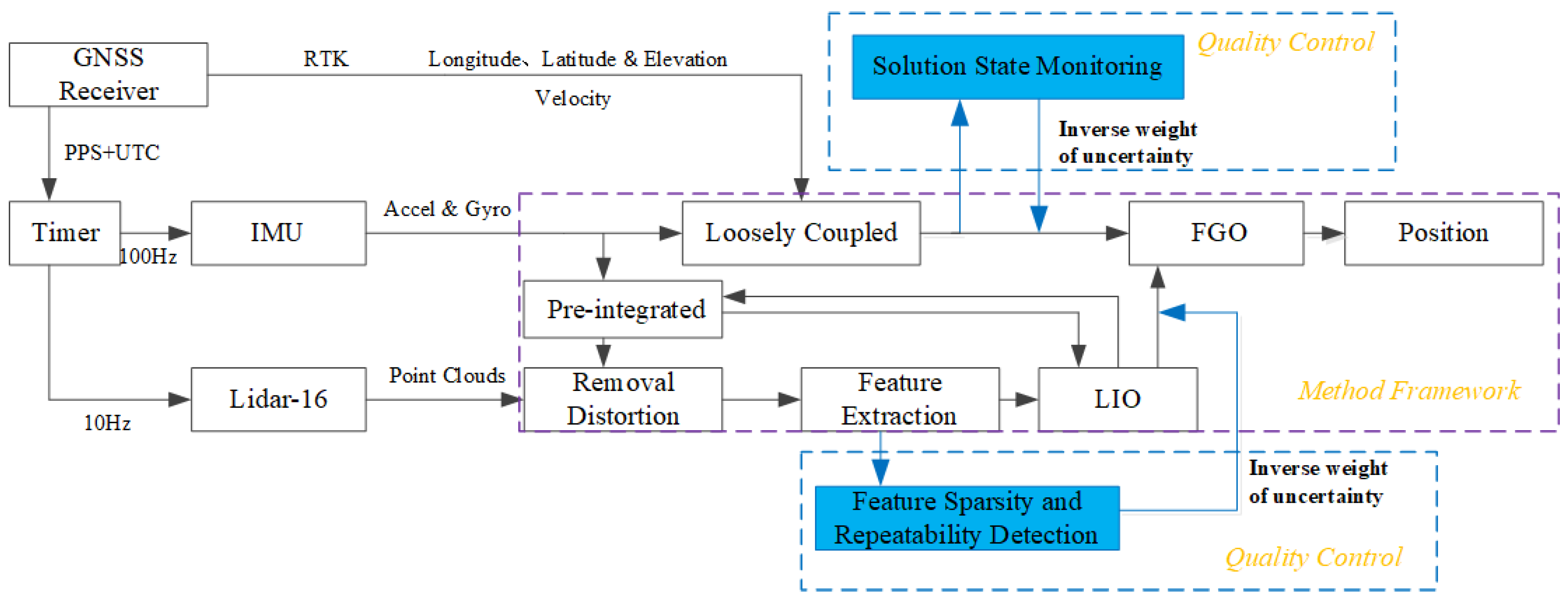
Figure 1. Framework of multi-source fusion algorithm based on quality control.
Remotesensing 17 03760 g001
Figure 2. Experimental platform system on the vehicle.
Remotesensing 17 03760 g002
Figure 3. (a) Positioning result of urban tunnels environment (WGS84 coordinate projection, Red Line): (A,B) is Tongjimen Tunnel; (C,D) is Xi‘anmen Tunnel; (b) mapping of Xi’anmen Tunnel.
Remotesensing 17 03760 g003
Figure 4. LiDAR feature quality assessment: (A,B) is the Tongjimen Tunnel; (C,D) is Xi’an men Tunnel.
Remotesensing 17 03760 g004
Figure 5. Inverse weight of sensor weights between LIO and GNSS/INS in urban tunnel positioning results.
Remotesensing 17 03760 g005
Figure 6. (a) Positioning result of urban environment (WGS84 coordinate projection, Red Line); (b) mapping of sections of the road.
Remotesensing 17 03760 g006
Figure 7. LiDAR feature quality assessment of urban environment.
Remotesensing 17 03760 g007
Figure 8. Inverse weight of sensor weights between LIO and GNSS/INS in urban positioning results.
Remotesensing 17 03760 g008
Figure 9. (a) Positioning result of Southeast University campus environment (WGS84 coordinate projection, Red Line); (b) mapping of campus.
Remotesensing 17 03760 g009
Figure 10. LiDAR feature quality assessment of campus environment.
Remotesensing 17 03760 g010
Figure 11. Inverse weight of sensor weights between LIO and GNSS/INS in campus positioning results.
Remotesensing 17 03760 g011
Figure 12. (a) Positioning result of mountain environment (WGS84 coordinate projection, Red Line); (b) mapping of sections of the road.
Remotesensing 17 03760 g012
Figure 13. LiDAR feature quality assessment of mountain environment.
Remotesensing 17 03760 g013
Figure 14. Inverse weight of sensor weights between LIO and GNSS/INS in mountain positioning results.
Remotesensing 17 03760 g014
Figure 15. (a) Accuracy assessment of campus environment mapping; (b) mapping of sections of the campus.
Remotesensing 17 03760 g015
Table 1. APE w.r.t Transition (m) [32] in different environments.
DatasetOURS
(With QC Module)
LIO_SAM
(Without QC Module)
LIO_SAM (gps)
(Without QC Module)
FAST-LIOLEGO_LOAM
RMSEMaxMinRMSEMaxMinRMSEMaxMinRMSEMaxMinRMSEMaxMin
Tunnel
(628s)
Continuous and smoothFalse (16s)False (7s)FalseFalse
Urban
(2014s)
0.180.480.01False (1133s)False (165s)False>1000
Urban
(180s)
0.140.240.1119.7328.9810.03False (74s)27.2263.863.04143.96196.9235.99
Campus
(180s)
0.230.290.151.822.581.220.490.770.244.178.131.701.311.860.92
Mountain
(760s)
0.211.760.01>1000False>1000>1000
False (ts) denotes the system degradation at time t. QC is the abbreviation of quality control.
Table 2. Repeatability statistics of LiDAR features for different scenes.
DatasetUrbanTunnelCampusMountain
GlobalPlanarEdgeGlobalPlanarEdgeGlobalPlanarEdgeGlobalPlanarEdge
σ d i f f 80.6679.3820.5123.7321.739.64999.194.6225119.311430
σ A 2.10%2.23%3.92%0.79%0.78%4.68%2.14%2.28%4.16%3.95%4.20%6.43%
Disclaimer/Publisher’s Note: The statements, opinions and data contained in all publications are solely those of the individual author(s) and contributor(s) and not of MDPI and/or the editor(s). MDPI and/or the editor(s) disclaim responsibility for any injury to people or property resulting from any ideas, methods, instructions or products referred to in the content.