Uncertainty Mixture of Experts Model for Long Tail Crop Type Mapping

Highlights

What are the main findings?

• The DMoE-ViT framework addresses the intra-class long tail problem by stratifying samples and employing a Vision Transformer-based multi-expert network, achieving an accuracy of 96.40%, a recall of 0.964, an F1-score of 0.964, and a Kappa coefficient of 0.960 in Study Area 1.
• Both qualitative and quantitative analyses confirm the robustness of this framework when addressing complex agricultural environments characterized by sample imbalance and intra-class variability.

What are the implications of the main findings?

• The DMoE-ViT framework enhances crop type mapping accuracy by addressing long tail distributions and employing a multi-expert network, thereby reducing overfitting and enabling precise crop mapping.
• By integrating uncertainty quantification techniques, the DMoE-ViT model enhances reliability, enabling precise crop monitoring under diverse environmental conditions.

Abstract

Accurate global crop type mapping is essential to ensure food security. However, large-scale crop-type mapping still poses challenges to commonly used classification strategies. Specifically, variation within crop types downgrades classification performance due to unbalanced samples with different levels of difficulty. Recent studies have focused on adaptive classification models based on sample difficulty to address challenges associated with complex crops grown under diverse conditions. However, these models still face challenges, as intra-class variability and imbalanced training samples lead to intra-class long tail distribution issues that affect performance. We propose the Difficulty-based Mixture of Experts Vision Transformer (DMoE-ViT) framework, which utilizes stratified sample partitioning, a multi-expert mechanism, and uncertainty quantification to address the long tail problem within a class and enhance classification accuracy. By assigning samples of varying difficulty to specialized expert networks, DMoE-ViT mitigates overfitting and enhances robustness, resulting in superior crop classification performance in complex agricultural environments. The DMoE-ViT framework outperforms baseline deep learning models, achieving an accuracy of 96.40%, a Recall of 0.964, an F1-score of 0.964, and a Kappa Coefficient of 0.960 in Study Area 1. Qualitative analysis of sample outputs and uncertainties, alongside quantitative evaluation of sample imbalance effects, demonstrates the framework’s robustness in complex agricultural environments.

1. Introduction

Agriculture is essential for sustaining human existence [1]. Humanity must urgently confront the majority of issues associated with food production [2,3,4]. Prompt and precise access to agricultural data can enhance crop management and address challenges related to food production and food security. Remote sensing supplants field surveys to acquire data on crop dynamics, offering an efficient method for mapping crop types on a large scale [5]. Specifically, due to the enhanced spatial and temporal resolution of remotely sensed imagery, it has emerged as the predominant technique for classifying crop types [6]. The efficacy of remote sensing technology for crop type identification is frequently limited by intraspecific variability due to uneven training samples, resulting in a long-tailed distribution of intraspecific data. This ultimately hinders the efficacy of classification methods and undermines the precision of crop mapping.

In recent years, significant progress has been made in crop classification [7]. Traditional methods, such as Random Forest [8] and Support Vector Machine (SVM) [9,10], rely on mono-temporal static spectral features, which make it challenging to adapt to dynamic changes during crop growth. With the development of deep learning techniques, particularly the application of Convolutional Neural Networks [11], classification accuracy has increased dramatically, and these models can effectively extract spectral-spatial feature representations for various crops. However, mono-temporal models overlook the temporal features of crop growth and cannot fully account for long-term trends and seasonal fluctuations [12,13,14]. To address this limitation, time-series-based deep learning models, such as LSTM [15] and Transformer [16], along with their variants [17,18], have emerged. These models utilise remote sensing time series that capture dynamic changes in the crop growth cycle, enabling the accurate analysis of both short-term fluctuations and long-term trends [19,20]. This analysis enhances classification accuracy, particularly when handling complex temporal dependencies [21]. In recent years, the application of the Transformer in remote sensing crop classification has expanded rapidly. It is not only used for sequence modelling but also for multimodal fusion and multi-scale feature extraction [17,18], significantly enhancing the representation ability of complex agricultural scenes. However, the improvement of agrarian classification accuracy depends not only on the classification method but also on the quality and quantity of training samples [22,23,24]. The boundaries of the training dataset are predominantly influenced by intra-class variability [25,26], arising from diverse growth conditions attributable to environmental factors (e.g., maize exhibiting varying phenological patterns due to topographical differences) [27]. These factors lead to significant differences in the spectral and temporal domains, even for the same crop type [25,28,29]. On the other hand, deep learning models tend to focus more on easily distinguishable samples while ignoring confusing or hard samples [30,31]. This leads to an overfitting phenomenon on easy samples during the training process, while the model may perform poorly on difficult ones [32]. The long tail distribution issue caused by unbalanced intra-class variation leads to overfitting, significantly reducing the model’s classification performance (i.e., increasing prediction uncertainty), particularly when dealing with complex crop environments in the real world. Therefore, we require a robust crop classification method that accounts for the long tail distribution of samples within classes to generate reliable crop mapping information. Recent studies have begun to focus on uncertainty modeling to alleviate the above problems. For instance, Ref. [33] proposed an uncertainty-aware dynamic fusion network (UDFNet), which quantifies the confidence level of multimodal remote sensing data using an energy function to achieve adaptive feature fusion and performs well in land cover classification with significant intra-class variation. Ref. [34] introduces dual-uncertainty (randomness and cognition) modelling for detecting architectural changes, significantly enhancing the Transformer’s robustness in scenarios with high intra-class variation. A systematic assessment of the uncertainty of the Earth observation segmentation model was conducted, verifying the effectiveness of the integrated and random reasoning methods in the semantic segmentation of satellite images, which can be transferred to the crop classification task [35].

To date, researchers have paid little attention to intra-class variation or unbalanced sampling, which leads to long tail distribution issues during model training and prediction for crop mapping tasks [27]. To address the problem of intra-class variation, Sun et al. classified winter wheat by leveraging a time series of vegetation indices to measure the similarity between crops [36]. Although this method can effectively capture crop growth characteristics, it still cannot adequately address the diversity of crop growth conditions and intra-class variability through time curves. Another strategy is to utilise biorhythmic features (quantified by measuring various biorhythms (e.g., start, peak, and end times) in the vegetation index time series) to improve crop classification performance. For example, Qiu et al. identified winter wheat by analysing the variations that occurred before and after the heading date [29]. However, the multivariate nature of biorhythmic features has not effectively solved the problem of intra-class sample variability. As intra-class variability increases, the feature space of crop samples becomes more complex, and the boundaries between samples gradually become blurred, resulting in unbalanced samples with varying levels of difficulty. Consequently, this variability is evident not only in the feature disparities within the spectral-temporal domain but also in the quantity of within-class samples across varying levels of difficulty. For instance, some samples may be more challenging to identify due to different growing conditions, such as on higher elevations, or even missing data in time series. To address these challenges, Zeng et al. optimised the sampling process by introducing an adaptive weight function that adjusts the sampling weights based on the degree of data imbalance, thereby significantly improving classification accuracy [37]. This enables the model to focus more on highly confusing and difficult-to-recognise samples while minimising its reliance on easily classifiable ones. This approach effectively mitigates the overfitting of easy-to-categorise samples while improving the model’s adaptability to handle “more difficult” samples. By incorporating an adaptive learning mechanism, the model can dynamically adjust its learning strategy in response to the crop’s growth conditions and environmental characteristics, thereby improving its classification ability for complex samples and enhancing the model’s robustness and generalisation ability. Although adaptive learning can improve crop mapping performance by focusing on complex samples, the imbalance between easy and hard sample instances still poses a challenge for single-branch deep learning frameworks. This is because single models typically rely on one-time, fixed decision boundaries. When confronted with imbalanced samples, those boundaries often fail to accommodate the diversity and complexity of sample feature representations [38,39].

Recent research has employed the Mixture-of-Experts (MoE) framework to tackle this issue. The MoE establishes a network of various specialists, each concentrating on a particular task or data subset, and employs a gating mechanism to select the appropriate experts for classification dynamically. This method can effectively manage sample heterogeneity and improve classification accuracy. In this respect, Lei et al. introduced a multi-level fine-grained crop classification method utilising multi-expert knowledge distillation to tackle classification issues arising from the similarity of crop biological parameters [40]. Nevertheless, conventional Mixture of Experts (MoE) encounters certain constraints when addressing extremely ambiguous or challenging data, particularly when intra-class difficulty differences are inadequately acknowledged. This may result in the incorrect assignment of hard samples to experts who are unsuitable for them. To overcome this problem, the MoE structure incorporates intra-class difficulty partitioning to ensure that multiple experts train complex samples with varying levels of difficulty. The more challenging examples are allocated to different experts for iterative learning and optimisation, enabling each expert to concentrate on samples of variable difficulty levels. This improvement effectively addresses the shortcomings of traditional MoE in dealing with intra-class sample variations, thereby enhancing the model’s performance in handling highly complex and confusing samples [41,42,43]. Despite these improvements, the MoE still faces the challenge of slow convergence, resulting from the conflicting predictions of multiple experts. Moreover, the introduction of numerous experts significantly expands the model’s parameter space, resulting in longer training times and increased computational resource consumption. To mitigate these problems, we incorporate an uncertainty measurement mechanism that dynamically adjusts the weighting factor by evaluating the prediction confidence of each sample. This innovation combines the strengths of the MoE with uncertainty quantification to provide a more efficient and accurate solution, especially in complex agricultural classification tasks.

We propose a Difficulty-based Mixture of Experts Vision Transformer framework (DMoE-ViT), which assigns intra-class samples of varying difficulty levels to different expert networks, enabling precise crop classification. The proposed framework consists of three main components: first, a stratified partitioning of samples based on their difficulty levels; second, a multi-expert mechanism to solve the long tail distribution problem caused by the imbalance in sample difficulty distribution; and finally, the incorporation of uncertainty analysis to further enhance classification accuracy. The main contributions of the research are as follows:

(1)

We propose a difficulty-induced sample quantification strategy to address the long tail distribution of intra-class sample difficulty, thereby improving the training performance of crop classifiers.

(2)

The multi-expert mechanism dynamically learns weights by focusing on samples at different difficulty levels, thereby improving crop mapping.

The rest of this paper is organized as follows: Section 2 introduces the proposed DMoE-ViT model. Section 3 describes the study area, along with the data collection and pre-processing methods for optical and SAR satellite time-series data. Section 4 details the experimental setup and model parameters. Section 5 presents the experimental results and their accuracy. Section 6 analyzes the labeling of the same sample by multiple experts and the effect of sample difficulty classification on the results. Finally, Section 7 concludes the paper.

2. Materials and Methods

2.1. Proposed Model for Fine Crop Mapping

The proposed DMoE-ViT model comprises three submodules. The first part is the Difficulty-based Long Tail Sample Classification Module, the second part is the Personalized Learning Module, and the last part is the Feature Filter and Classification Module, as shown in Figure 1.

Figure 1 presents a schematic overview of the proposed three-stage crop classification framework. In the first Stage (Difficulty-based Long Tail Sample Classification Module), pre-processed remote sensing data is reconstructed using an encoder–decoder architecture, where samples are automatically categorised into easy, moderate, or hard groups based on their reconstruction loss—a detailed formulation of which is provided in Section 2.2. The second Stage (Personalized Learning Module) dynamically routes these difficulty-grouped samples to three specialized Vision Transformer (ViT) experts: Expert 1 (x₁) receives all samples, Expert 2 (x₂) processes moderate and hard samples, and Expert 3 (x₃) focuses exclusively on hard samples. A trainable gating mechanism G(x) adaptively fuses features extracted by these experts within a Mixture-of-Experts (MoE) structure. Finally, the third Stage (Feature Filter and Classification Module) incorporates an uncertainty estimation module that identifies high-uncertainty samples from the fused features, subsequently refining the feature representation and calibrating the classification output to enhance robustness and accuracy.

2.2. Difficulty-Based Long Tail Sample Classification Module

As shown in the first module of Figure 1, we present a difficulty-aware classification pipeline based on an autoencoder. This pipeline employs a CNN-based encoder–decoder architecture, where the encoder progressively compresses the input image into bottleneck-layer features through successive stacks of convolutional layers, batch normalisation, and activation functions. The decoder, in turn, reconstructs the original image from these features using inverse operations such as deconvolution.

The core of this design lies in utilising reconstruction loss as a quantitative metric for assessing sample difficulty, with its theoretical foundation rooted in the inherent learning characteristics of autoencoders. During training, the autoencoder preferentially fits the distribution patterns of the most frequently occurring samples in the dataset. This property enables reconstruction loss to effectively reflect the representational difficulty of a sample relative to the current model and task: for standard samples that align with the learned distribution, the model achieves accurate reconstruction with low loss values; in contrast, for anomalous samples that deviate from the dominant patterns, reconstruction error rises significantly due to insufficient feature representation capacity. Thus, the magnitude of the reconstruction loss directly reflects the degree to which a sample’s features deviate from the dominant distribution, naturally serving as a reliable measure for difficulty stratification: higher reconstruction loss indicates greater learning difficulty, thereby enabling effective differentiation between easy and hard samples in long tail data distributions. Treating X as the set of all sample instances, where each instance $x\in X$, given a finite training set with index $m$ consisting of only a few samples $(x^m,l^m)$,$l^m\in L=\{1,\dots ,|K\left|\right\}$ is the label index for $x^m$, K represents the number of classes. Multiple convolutional layers, along with batch normalization (BN) and rectified linear units (ReLU), work together as an effective encoder $f_e(·)$ to extract spectral-spatial features z from the samples [44].

$$z=f_e\left(x\right)$$

(1)

In the encoder, the output of a convolutional layer ${\mathrm{\varnothing }}_{conv}(·)$ can be simplified as

$$x_{{\mathrm{f}}_{conv}}=f_{conv}\left(x\right)$$

(2)

After being processed by BN, ReLU activation function, and Conv, the input $x_{{\mathrm{\varnothing }}_{conv}}$ undergoes normalization, activation, and convolution sequentially to extract richer feature representations.

$$z=Conv\left(ReLU\left(BN\left(x_{f_{conv}}\right)\right)\right)$$

(3)

To enable the network to directly distinguish the difficulty of long tail samples within each class, we introduce a reconstruction task. We compute the reconstruction loss by comparing the reconstructed image with each instance x, and we assess the difficulty of the long tail sample based on the magnitude of this loss.

$$\widehat{x}=fr\left(z\right)$$

(4)

where $\widehat{x}$ is the reconstructed instance, $fr(·)$ is the reconstruction function or named the decoder, and y is the output latent features from the encoder $f_e(·)$. Here, we utilize the L2 norm as the reconstruction loss, which quantifies the difference between the original input sample and its reconstruction. Smaller values of this loss indicate better reconstruction quality.

$$dist\left(x,\widehat{x}\right)=\sqrt{\sum _{j=1}^n{\left(x-\widehat{x}\right)}^2}$$

(5)

In the decoder, the key element is the deconvolutional layer, also called the transposed convolutional layer. We consider it as the inverse of a convolutional layer, denoted as ${\mathrm{\varnothing }}_{conv}^T(·)$, resulting in

$$x={\mathrm{f}}_{conv}^T\left({\mathrm{f}}_{conv}\left(x\right)\right)$$

(6)

The transposed convolution operation in this model transforms the image from low-resolution feature maps to high-resolution images, enabling the network to perform the reconstruction task more effectively. This allows the network to learn and assess the complexity of the input images during the training process. In the autoencoder-based difficulty-aware classification pipeline, the reconstruction loss serves as an unsupervised mechanism for quantifying sample complexity, allowing the network to accurately assess the complexity of each sample and differentiate between difficulty levels during training. We achieve this through three key advantages: (1) it eliminates the need for manual prior annotations, thereby avoiding subjective bias; (2) its deep integration with the feature learning process allows dynamic capture of anomalies in sample distribution; and (3) it provides a continuous and differentiable difficulty metric that supports differentiated learning strategies based on the difficulty spectrum. By identifying high-difficulty samples via elevated reconstruction loss, the network can adaptively adjust its learning strategy. This difficulty stratification mechanism not only enhances the model’s ability to recognise and handle challenging samples but also significantly improves overall generalisation performance on long tail data distributions.

2.3. Mixture of Experts Classification Module

Figure 2 details the architecture of the Personalised Learning Module (Stage II) and its integration with both the preceding Difficulty-based Long Tail Sample Classification Module (Stage I) and subsequent Feature Filter and Classification Module (Stage III). The module takes as input the complete set of study area samples, pre-categorised in Stage I using reconstruction loss into easy, moderate, and hard subsets. These subsets are strategically reorganised into expert-specific datasets xᵢ (where i denotes expert index), following our specialised distribution scheme: Expert 1 processes all samples (x₁), Expert 2 handles moderate and hard samples (x₂), and Expert 3 focuses exclusively on hard samples (x₃). Each expert network processes its respective dataset, and we adaptively fuse the extracted features through a trainable gating mechanism G(x). We forward the integrated features to Stage III, where we perform uncertainty estimation to identify high-uncertainty components and apply selective weighting to refine the final feature representation for optimal classification performance. This design enables targeted processing of samples according to their difficulty levels while maintaining feature coherence through learned fusion and uncertainty-based calibration.

The core idea of the Mixture of Experts (MoE) model is to assign input data to different “expert” networks based on different features, and the “gating network” determines the contribution weight of each expert. We show the structure diagram of the model in Figure 2, and we divide its main formulas into the following parts: The MoE model consists of multiple expert networks, where each expert, $E_i$ is an independent sub-network that focuses on specific features or tasks. Through independent training, each expert learns more targeted feature representations, adapting to different types of data inputs.

Let there be M experts, where each expert network $E_i$ produces a prediction based on the input x:

$$y_i=E_i\left(x\right),i=\mathrm{1,2},\dots ,M$$

(7)

The primary function of the gating network is to dynamically assign weights to each expert based on the input data x. It uses a neural network to compute the weights $g_i\left(x\right)$, which represents the importance of each expert $i$ in the final output. The output of the gating network is typically normalized using the softmax function, ensuring that the sum of all weights is equal to 1, thereby facilitating a weighted average, as described by the following condition:

$$\sum _{i=1}^M{g}_i\left(x\right)=1$$

(8)

2.3.1. Single Expert Learning Process

For the data allocation strategy in expert networks, we designed a structured data routing mechanism to establish a division-of-labour system that progresses from easy to complex tasks. Given a training set, where X represents the data and Y represents the corresponding labels, the samples are classified into three categories based on difficulty: easy, moderately easy, and difficult, denoted as $\{n_1,n_2,n_3\}$. The experts are $\{E_1,E_2,E_3\}$, with a total of 3 experts. We evenly divide the three categories of samples into three subsets based on the number of experts and denote them as ${\theta }_1=\{D_1,D_2,D_3\}$ [45]. The training data for different experts is allocated based on the difficulty level of the long tail samples. The data assigned to the expert $E_1$ is denoted as ${\theta }_1=\{D_1,D_2,D_3\}$, the data assigned to the expert $E_2$ is denoted as ${\theta }_2=\{D_2,D_3\}$, and the data assigned to the expert $E_3$ is denoted as ${\theta }_3=\left\{D_3\right\}$, which is expressed as

$${\theta }_i=\left\{\begin{array}{c}\left\{D_1,D_2,D_3\right\}, i=1\\ \left\{D_2,D_3\right\}, i=2\\ \left\{D_3\right\}, i=3\end{array}\right.$$

(9)

Specifically, Expert E₁ utilises the entire dataset {D₁, D₂, D₃} to establish a general feature base; E₂ employs {D₂, D₃} to focus on discriminative features for moderate-to-hard difficulty samples; E₃ exclusively uses {D₃} to specialise in learning sparse discriminative features within hard samples. In this approach, the network training focuses on moderate and hard samples. Each network can specialise in its respective data characteristics by providing different datasets of varying difficulty to different expert networks, thereby enhancing recognition performance and improving learning efficiency.

For each expert, the Vision Transformer (ViT) model processes an input image $X\in {\mathbb{R}}^{H\times W\times C}$ by dividing it into $N={\displaystyle \frac{H}{P}}\times {\displaystyle \frac{W}{P}}$ fixed-size patches, where H, W, and C denote the height, width, and number of channels of the input image, respectively, and P is the patch size. Each patch $X_i\in {\mathbb{R}}^{P\times P\times C}$ represents a spatial region of size $P\times P$ pixels across all C channels, allowing the model to recognise detailed features in the local areas. This approach avoids the limitations of local convolutional kernels in traditional convolutional neural networks (CNNs) and enhances the ability to extract global features. To efficiently learn the key information from each patch, the ViT model applies a linear transformation to compress the high-dimensional features of each patch into a lower-dimensional embedding vector [46].

$$Z_i=Linear\left(Flatten\left(X_i\right)\right)$$

(10)

Considering that the growth patterns and spatial distribution of crops are typically closely related to their position in the image, the ViT model also adds positional encoding (PE) to the embedding vectors $Z_i$ of each patch, resulting in a positionally encoded embedding matrix.

$$Z^{\text{'}}=Z_i+PE$$

(11)

PE helps to understand the layout and relative positioning of crops in the imagery, as well as to distinguish subtle differences between different species more effectively. Nonetheless, considerable variety frequently exists in the morphology, hue, and growth duration of crops in remotely sensed photography, typically linked to the spatial dependency of geographic locations. Using the self-attention mechanism, the ViT model can better capture the relationships between these regions. It processes the positionally encoded embedding matrix $Z^{\text{'}}$ using a Transformer structure, producing a global feature matrix $H_{enc}$,

$$H_{enc}=Transformer\left(Z^{\text{'}}\right)$$

(12)

which effectively captures global information from the image. To aggregate the local features from all patches, the ViT model employs global average pooling (GAP) to summarise all patch features into a single global feature vector for the entire image.

$$\mathrm{v}=\mathrm{G}\mathrm{A}\mathrm{P}\left(H_{enc}\right)$$

(13)

This enables the model to integrate local information from each patch into a global representation, allowing for crop classification based on overall global features. Finally, the ViT model inputs the global feature vector v into a fully connected layer and outputs the probability distribution for each crop class through a Softmax function,

$$\widehat{y}=Softmax\left(W·v+b\right)$$

(14)

where W and b are the weight matrix and bias term of the classification layer, respectively, completing the crop classification task. The final model output $y_{moe}$ is the weighted average of each expert’s output $y_i$ from each expert, i.e.:

$$y_{moe}=\sum _{i=1}^M{g}_i\left(x\right)·y_i$$

(15)

2.3.2. Estimating Evidence-Based Uncertainty

By introducing uncertainty evaluation, the model can identify samples with higher uncertainty, reduce its reliance on these samples, and more effectively allocate weights during training, thereby focusing on distinguishing subtle differences between classes and improving classification accuracy. Therefore, for intra-class sample classification, we introduce evidence-based uncertainty (EvU) under the Dempster-Shafer theory (DST) to enhance both confidence and efficiency [47].

DST is an extension of Bayesian probability theory, designed to better handle uncertainty and ambiguous information. Unlike the Bayesian approach, DST not only provides the probability of an event but also measures how much we believe in that event. Subjective logic (SL) is based on DST and focuses on the reliability of information sources and cognitive uncertainty. In DST, the quality of beliefs represents confidence in each category, with the total quality of beliefs summing to 1. Higher quality of beliefs indicates a greater likelihood that the category is correct. We consider a uniform distribution of belief quality across multiple categories to demonstrate a high degree of uncertainty in the prediction. Formally, the subjective logic defines the belief assignment over a Dirichlet distribution:

$$D\left(p|\alpha \right)={\displaystyle \frac{1}{B\left(\alpha \right)}}\prod _{k=1}^K\begin{array}{c}{p}_k^{{\alpha }_k-1} for p\in {∆}_k, and 0 otherwise\\ \end{array}$$

(16)

The parameters $\alpha$ define the distribution, while B(·) represents the Beta function, and ${∆}_k$ represents the Beta function, and $p_1+p_2+\dots +p_K=1 and p_k\ge 0$ for each k. The level of uncertainty is governed by these parameters, as follows:

$$u={\displaystyle \frac{K}{S}} and b_k={\displaystyle \frac{{\alpha }_k-1}{S}}$$

(17)

where K denotes the number of classes, $S={\sum }_{k=1}^K{\alpha }_k$ represents the Dirichlet strength, and ${\alpha }_k=e_k+1$ is the Dirichlet parameter for the k-th class with $e_k$ being its corresponding evidence. The evidence of each class $e=[e_1,e_2,\dots ,e_K]$ can be obtained directly from the output of neural networks by replacing the softmax layer with a non-negative activation function. The uncertainty mass u decreases as the total evidence strength S increase, while the belief mass $b_k$ for each class scales with its respective evidence. This formulation ensures $u+{\sum }_{k=1}^K{b}_k=1$, providing a theoretically grounded approach to uncertainty estimation that avoids over-confidence by considering the distribution of evidence across all classes rather than relying solely on predicted probabilities.

After weighting the output of each expert through the MOE gating mechanism $g_i\left(x\right)$ to obtain the final result $y_{moe}$ of MOE, the uncertainty $u_i$ of each expert’s output is added. The result is

$$y=\sum _{i=1}^M{g}_i\left(x\right)·y_i·u_i$$

(18)

During training, the loss function of the MoE model is typically the weighted sum of the losses from all experts, given by:

$$L=\sum _{i=1}^M{g}_i\left(x\right)·L_i\left(y_i,y_{true}\right)$$

(19)

Among them, $L_i$ represents the loss of the i-th expert, and $y_{true}$ is the true label. The MoE model employs a gating network to direct the input data to select different experts, thereby effectively handling complex tasks and enhancing the model’s generalization ability.

We propose a novel Mixture-of-Experts (MoE) network that, through a meticulously designed data allocation strategy, establishes a differentiated dominance pattern across experts for easy, moderate, and hard samples. This architecture fully exploits the pronounced feature disparities in crop classification tasks—manifest in shape, color, and texture—by integrating three pivotal mechanisms to ensure model efficacy: First, a gating network dynamically evaluates sample difficulty and adaptively assigns expert weights; second, shared low-level parameters maintain feature space consistency, supplemented by regularization to mitigate overfitting; and third, an uncertainty-weighted ensemble calibration is introduced during inference to refine the integrated output. This synergistic framework effectively alleviates the underrepresentation of hard samples in long tail data, preserving baseline classification performance while significantly enhancing recognition accuracy for moderate- and high-difficulty instances.

3. Study Areas and Data Acquisition Instructions

3.1. Introduction to the Study Areas

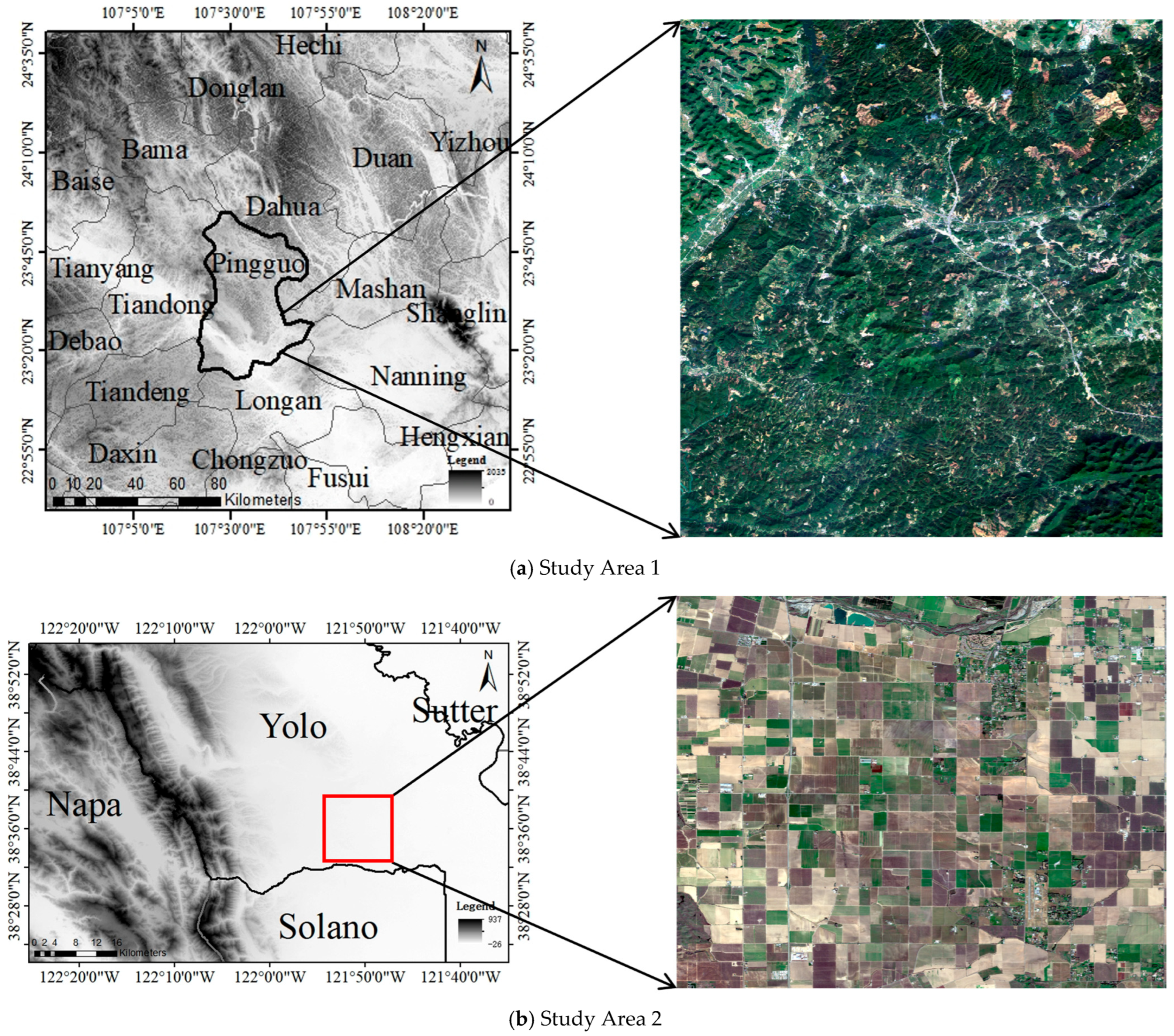
The first study area is located in Pingguo City, in the western region of Guangxi Province, which Baise City governs. The geographical coordinates are 107°21′ to 107°51′ east longitude and 23°12′ to 23°51′ north latitude. It is one of the locations characterised by intricate and varied agricultural planting systems in China. Pingguo City contains a varied topography, distinguished by mountains, hills, and river valleys. The terrain is significantly fragmented, characterised by a variety of farming types, predominantly featuring dry land. The region is a low-latitude tropical zone, located on either side of the Tropic of Cancer, distinguished by a typical subtropical monsoon climate. Both bright and rainy conditions characterize summers, while winters are warm. Precipitation predominantly occurs from May to September, creating optimal conditions for agricultural development in terms of water and temperature. in Pingguo City, agrarian land accounts for almost one-fourth of the county’s total area, primarily located in the northern, western, and southeastern regions. The predominant type is dryland, succeeded by paddy fields and a small proportion of wetland. The principal crops include rice, corn, sugarcane, and citrus fruits.

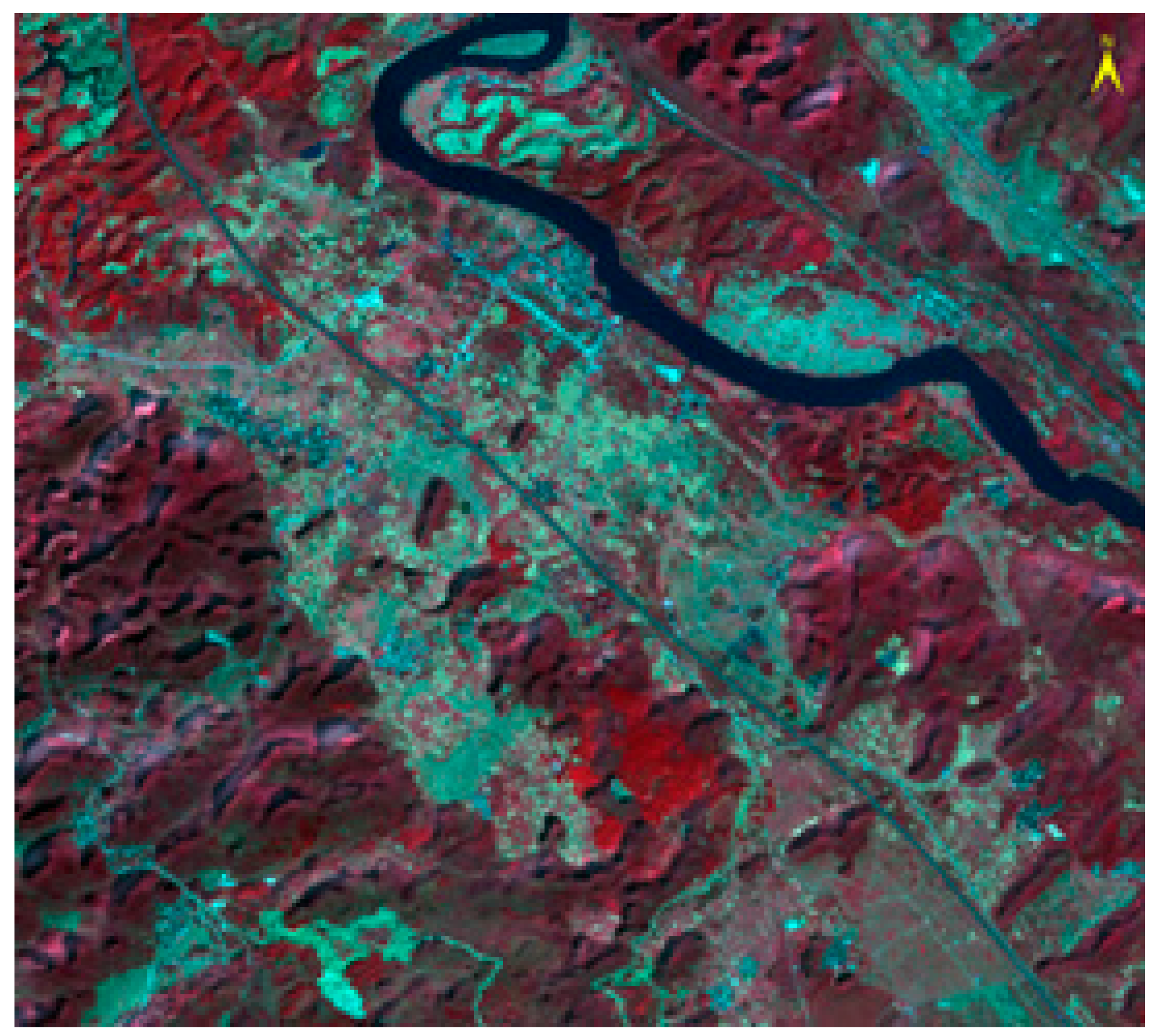
The second research area is located in the Sacramento Valley region of central California, USA. The area adjoins Sacramento and Napa counties and is situated within California’s Central Plains. The region is recognised for its arable land and is a significant agricultural zone in California. Yolo County exhibits a temperate Mediterranean climate, marked by moderate, moist winters and arid, sweltering summers. The region’s agriculture is highly diverse, yielding several cash crops, including almonds, grapes, tomatoes, olives, and lucerne. Grape and almond production significantly bolsters the local agricultural economy. Figure 3 illustrates the physical and geographic distribution of the two regions. Figure 3 illustrates the geographical and landscape characteristics of the two study regions: (a) Study Area 1 and (b) Study Area 2.

3.2. Data Acquisition Methods and Image Pre-Processing

3.2.1. Satellite Time-Series

This study utilized the interferometric wide swath (IW) observation mode and dual-polarization (VV + VH) ground range detection (GRD) products of Sentinel-1, which are available through the Google Earth Engine (GEE) remote sensing cloud platform (COPERNICUS/S1_GRD). The proposed method uses two characteristic representations of Sentinel-1 (S1) data: backscatter and polarization-decomposed data. The data format used is the SLC format in the interferometric wide swath IW scanning mode. All data utilised were obtained from the NASA Alaska Satellite Facility (ASF) Data Centre, encompassing the period from January to December 2023. The images were multi-look processed, thermal noise removed, radiometrically calibrated, and terrain corrected. In the study area 1, 25 available Sentinel-1 images were acquired throughout the year, including 25 vertical-vertical polarization backscatter VV images and 25 vertical-horizontal polarization backscatter VH images. In the study area 2, a total of 56 available Sentinel-1 images were acquired throughout the year, including 56 vertical-vertical polarization backscatter VV images and 56 vertical-horizontal polarization backscatter VH images.

The optical data used in this study comes from Sentinel-2 (S2), and the data format is atmospherically corrected Level-2A. The COPERNICUS/S2_SR data is declouded (images with cloud cover greater than 15% are removed), and the corresponding normalized difference vegetation index (NDVI) image is calculated. Considering factors such as image acquisition orbit and cloud cover, the images of Study Area 1 are merged into a synthetic image every six months to obtain two images for the whole year; the images of Study Area 2 are merged into a synthetic image every quarter to get four images for the entire year, from which NDVI is extracted. The NDVI calculation formula is as follows:

$$NDVI={\displaystyle \frac{{\rho }_{B8}-{\rho }_{B4}}{\left({\rho }_{B8}+{\rho }_{B4}\right)}}$$

(20)

In the formula, ${\rho }_{B8}$ and ${\rho }_{B4}$ represent the NIR and Red bands of the S2_SR dataset, respectively. Figure 4 shows the temporal distribution of different data types in the two study areas. By stacking the pre-processed Sentinel imagery, including NDVI, VV, and VH bands at three hierarchical levels (upper, middle, and lower), a multidimensional composite image was ultimately obtained.

3.2.2. Ground Reference Data

Crop type data for Pingguo City, Guangxi, were provided by the relevant and presented in vector data format. The crop types include seven categories: corn, sisal, citrus, dry rice, double-season rice, early rice, and sugarcane. Alternative land cover types, including structures and natural flora, were sourced from the Google Earth Engine (GEE) data product (https://developers.google.com/earth-engine/datasets/catalog/GOOGLE_DYNAMICWORLD_V1, accessed on 24 September 2025), yielding three classifications: buildings, woodland, and grassland. Using 2 m high-resolution imagery of Pingguo City, Guangxi, as reference data, the crop types in Pingguo City were divided into 10 distinct classes. To create the sample set for crop types from vector data, the total area of each crop planting region was initially computed, and the number of points to be allocated within each region was established based on this total area. These points served as labels. The points were transformed into pixel points using ArcMap 10.8 software and subsequently exported as TIFF images to function as label maps. In the spatial domain, square image patches of defined dimensions were randomly extracted along the temporal axis, with the central pixel associated with the CDL data assigned as the label. A segment of the label data was obtained from the 10 m classification product of the Google Earth Engine (GEE) platform. By acquiring the CDL imagery for 2023, various crop types were identified, and the corresponding target numbers for each type were extracted to generate image patch sample labels. These generated labels were subsequently entered into the model suggested in this study for training and prediction.

3.2.3. Sample Set Generation and Division

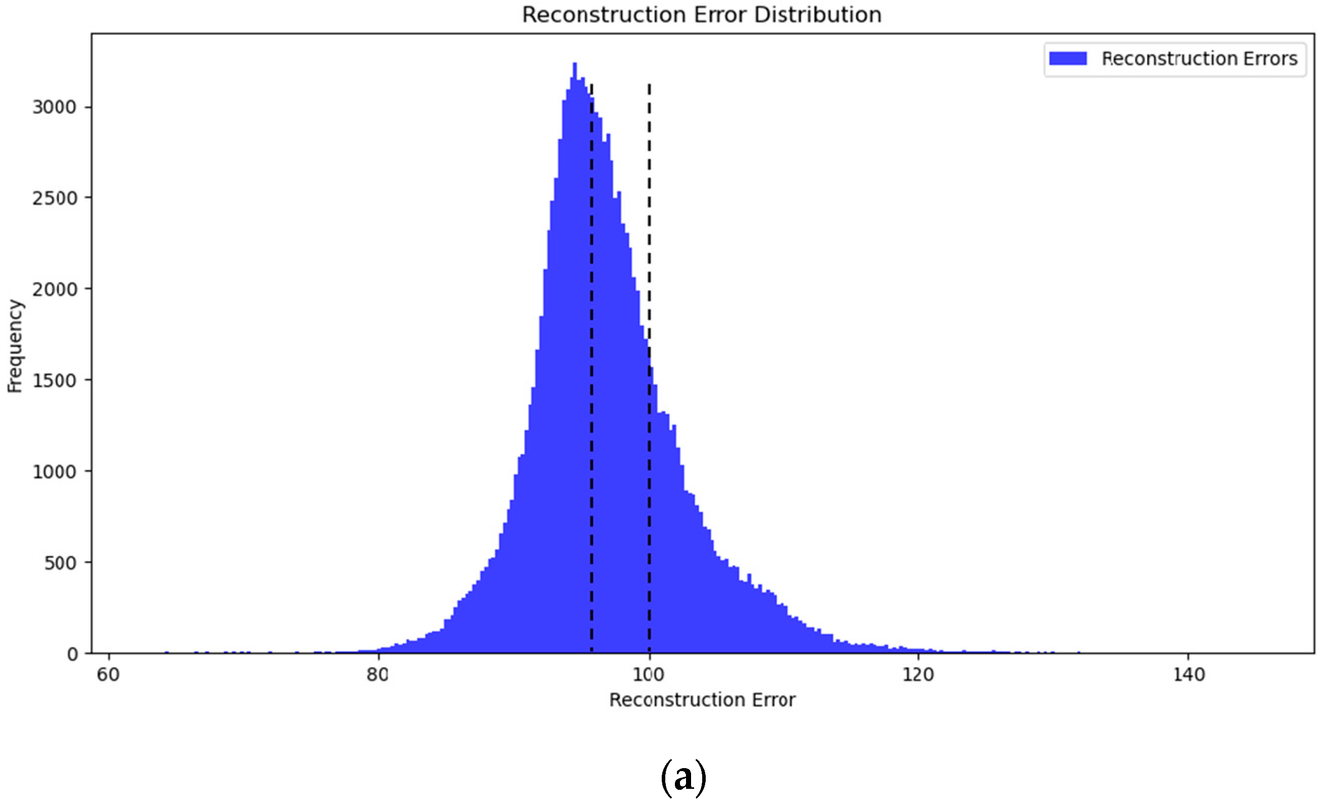
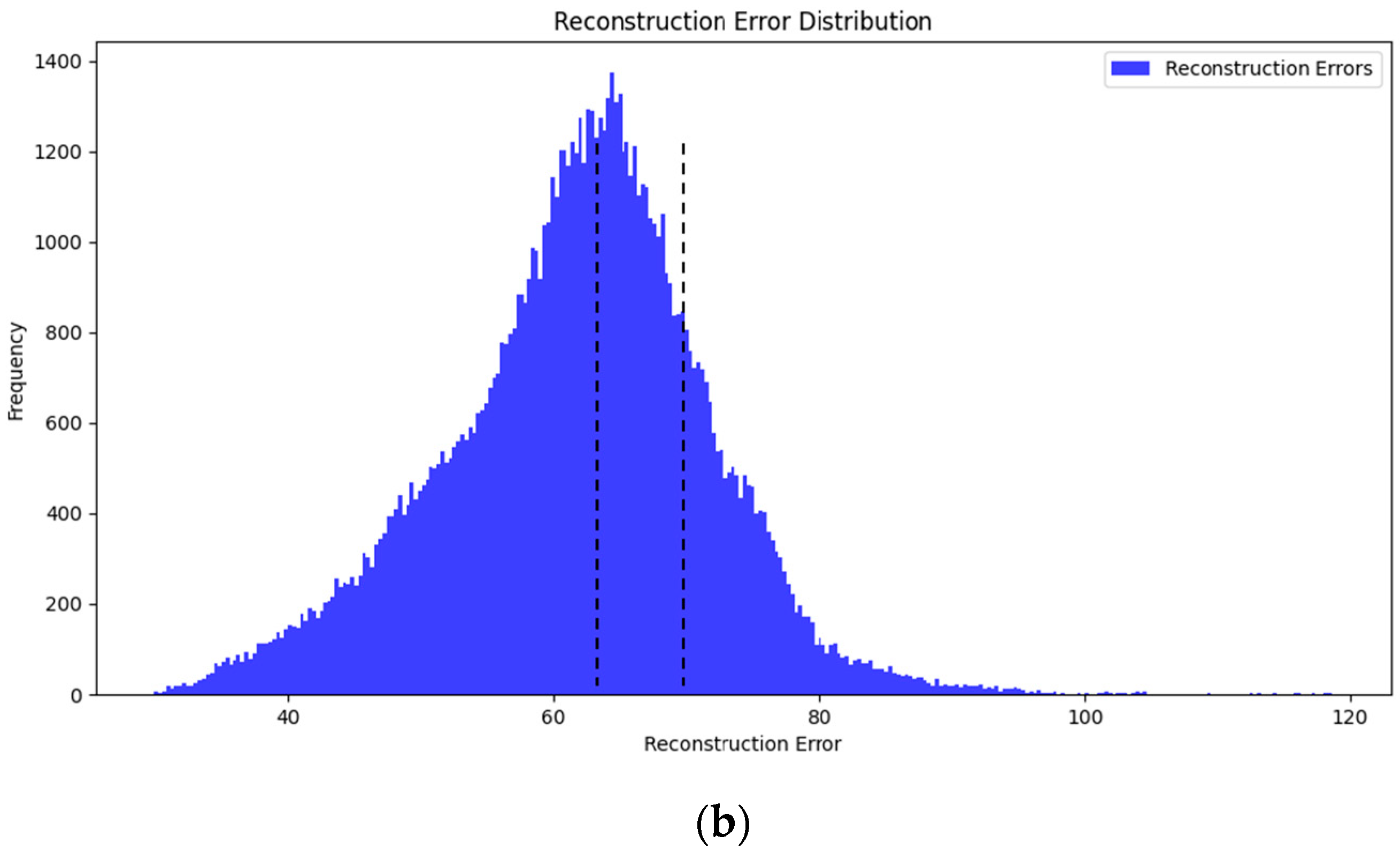
The area of various crops in the two research regions was evaluated using ground reference data. The primary crops in Research Area 1, determined by their area proportion, were identified as corn, sugarcane, sisal, citrus, dry rice, double-season rice, early rice, grassland, and woodland. Conversely, the predominant crops in research area 2 included corn, rice, sunflower, winter wheat, alfalfa, other hay types, tomatoes, fallow land, almonds, walnuts, developed land, plums, low-density regions, pastures, and olive trees. The “others” encompass crops beyond the primary categories (e.g., citrus, chickpeas, rye, cherries), resulting in a more complex class composition. Subsequently, random sampling was conducted in each research region, and 18 × 18 patches were extracted with the designated sites as the center for analysis. The retrieved samples were partitioned into distinct training and validation sets at an 80:20 ratio. The complexity level of each sample (easy, moderate, or hard) was ascertained by the reconstruction loss. The difficulty levels of long tail samples in Study Area 1 and Study Area 2 are classified according to a 3:2:1 ratio of sample quantities, as indicated by the dashed lines in Figure 5.

Table 1. Sample set distribution in the study area. Based on the magnitude of reconstruction loss, samples in each category are divided into three difficulty levels—easy, moderate, and hard—according to their quantitative proportions.

Area 1				Area 2
Classes	Easy	Moderate	Hard	Classes	Easy	Moderate	Hard
Corn	1090	721	285	Others	3336	2483	2029
Buildings	923	751	418	Corn	3879	2263	1821
Sisal	1160	545	386	Rice	4563	1738	1508
Citrus	1034	807	247	Sunflower	3685	2451	1732
Dry Rice	1060	600	429	Winter Wheat	3333	2455	2059
2S-Rice	622	516	512	Alfalfa	3421	2139	2072
Early Rice	698	576	562	OtherHay	5268	1677	581
Sugar Cane	1146	710	240	Tomatoes	3134	2546	2089
Grassland	1044	815	236	Fallow	3879	2510	1601
Woodland	940	646	514	Almonds	3352	2906	1625
				Walnuts	3430	3223	1208
				Dev-OpenSpace	3301	2511	2168
				Prunes	2829	2562	2469
				DevLowIntensity	3216	2844	1804
				Grassland Pasture	4342	2268	1217
				Olives	5599	1284	921

illustrates the number of samples for each difficulty level associated with the crop type.

4. Experimental Design

To better evaluate the proposed method’s classification performance, we compared it with five currently used deep learning networks: CNN, LSTM, CNN-Attention (CNN-Att), UNet, and ViT. Finally, we give a method for evaluating the model’s classification results.

4.1. Experiment Parameter Setting and Configuration

We first set the sample crop size of the proposed model to 18. Each expert uses 2D convolution to extract spatial information from the input samples. For the temporal feature extraction of crops, based on experimental findings and existing data, the encoder depth is set at 2, the number of MSA heads is fixed at 12, and the FFN input nodes are preset to 1296.

All models mentioned above are trained using the PyTorch 2.0 framework, with Adam as the optimiser, an initial learning rate of 0.00001, a batch size of 96, and a training duration of 35 epochs. Model training is conducted on a server utilising the CentOS 7.6 operating system, which is equipped with two NVIDIA Tesla V100 GPUs (16GB) and an Intel Xeon^® Gold 5118 CPU. Utilisation of Python version 3.6 is indicated.

4.2. Model Evaluation Methods

To better analyze the classification results and model capabilities, we used five commonly used accuracy assessment metrics: overall classification accuracy (OA), kappa coefficient, confusion matrix, F1-score, and Recall. OA indicates the proportion of correctly classified samples among all samples and is used to assess the classifier’s performance. The kappa coefficient reflects the consistency of the classification results, while the confusion matrix shows the classification performance for each crop type. The F1-score combines precision and Recall and is defined as their reconciled mean. Recall is a standard metric for assessing the performance of classification models.

5. Result

5.1. Ablation Experiments

5.1.1. Evaluating the Impact of Expert Framework on Classification Model Performance

This study compares the performance of traditional Convolutional Neural Network (CNN) and Vision Transformer (ViT) in crop classification, with a focus on evaluating the impact of these two architectures on classification accuracy. As shown in Figure 6 and Figure 7 and

Table 2. Ablation experiment results of study area 1.

Classes	ViT + MOE + Uncertainty	CNN + MOE + Uncertainty	ViT + MOE
Corn	100.00%	98.10%	99.80%
Buildings	86.80%	97.50%	87.20%
Sisal	100.00%	86.40%	99.20%
Citrus	100.00%	99.00%	100.00%
Dry Rice	96.50%	90.20%	99.40%
Double-season Rice	99.30%	71.60%	97.50%
Early Rice	97.40%	84.70%	91.60%
Sugar Cane	99.80%	83.70%	99.80%
Grassland	89.30%	83.60%	85.00%
Woodland	100.00%	98.10%	100.00%
OA	96.40%	89.70%	96.00%
Recall	0.964	0.869	0.960
F1-score	0.964	0.875	0.960
Kappa	0.960	0.854	0.955

using a CNN instead of the ViT model significantly reduces classification accuracy. While CNN excels at extracting local features and processing low-dimensional image data, it is inferior to ViT in managing crop classification tasks that involve intricate spatial patterns and long-range connections. ViT, with its self-attention mechanism, effectively captures global information and spatial linkages within images, offering a significant advantage, especially in differentiating complicated categories with nuanced distinctions.

In contrast to CNNs, which rely on localized convolution operations, ViT can recognize long-range correlations within the image, resulting in enhanced classification accuracy. In categories such as Double-season Rice and Sugar Cane, which exhibit intricate spatial interactions, ViT has improved classification capabilities. CNN concurrently fails to capture global information, leading to diminished classification accuracy.

5.1.2. Evaluating the Impact of Uncertainty on Classification Model Performance

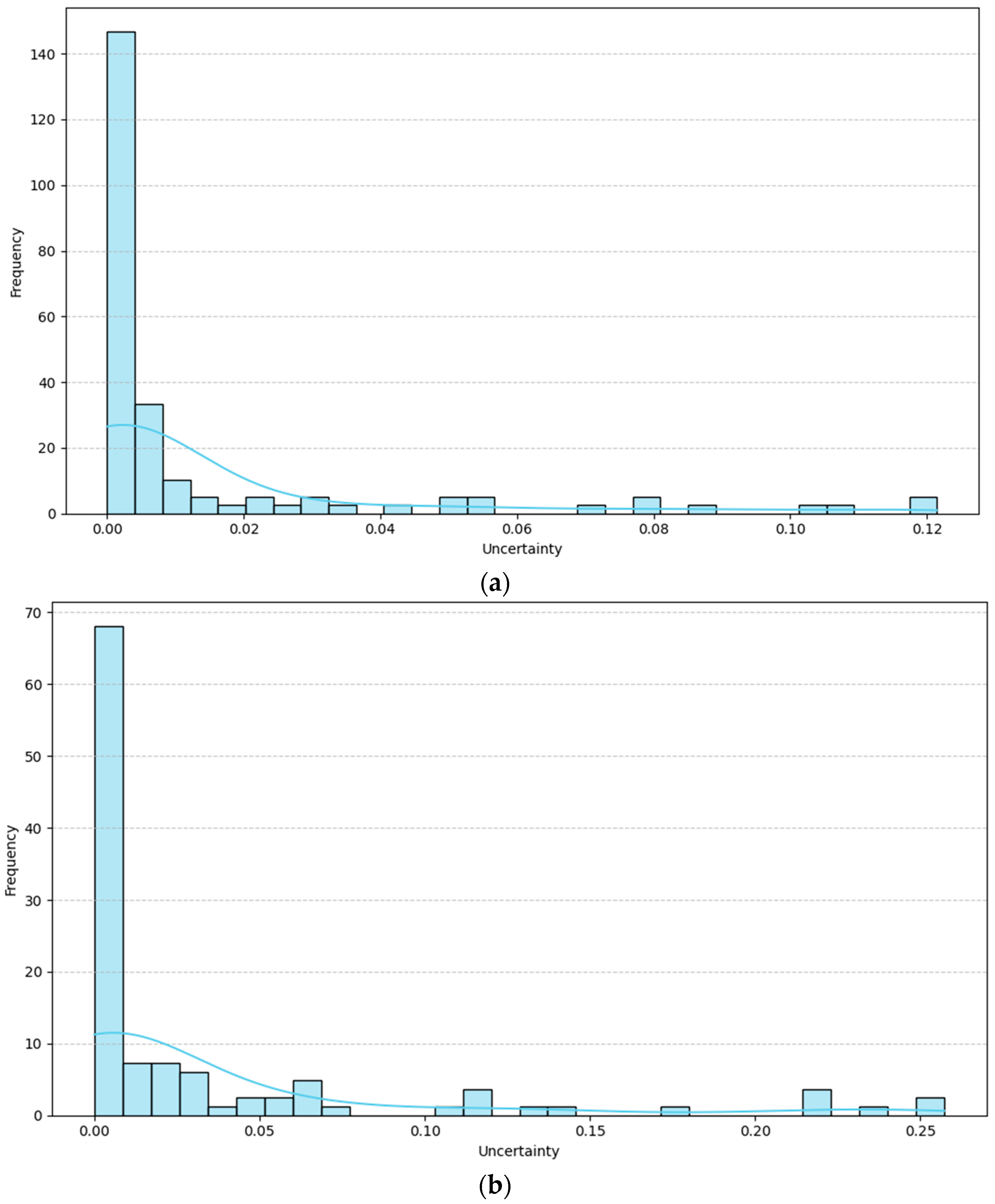
In this experiment, we evaluated the efficacy of models with and without the uncertainty weighting module in crop classification tasks. The experimental findings indicate that integrating the uncertainty weighting module significantly enhances the model’s performance across several measures, particularly in differentiating categories with similar characteristics. The model’s inability to dynamically modify weights according to the confidence or uncertainty of each output hindered its capacity to manage complicated or related categories, thus affecting classification accuracy. Particularly in multi-class classification or challenging tasks, incorporating an uncertainty weighting mechanism enabled the model to more effectively adjust to the varying significance of samples across multiple categories, resulting in a notable improvement in classification accuracy. As shown in Figure 8, after adding the uncertainty weighting, the uncertainty distribution of the model’s final output decreased, demonstrating the crucial role of this module in optimizing the model’s output. Specifically, the incorporation of the uncertainty module significantly enhanced the model’s classification accuracy across most classes. For example, classes like Corn, Sisal, and Citrus achieved 100% accuracy, while other categories, such as Grassland and Double-season Rice, also showed varying degrees of improvement.

Furthermore, the overall accuracy (OA), Recall, F1-score, and Kappa value all increased from 0.960, 0.960, 0.960, and 0.955 to 0.964, 0.964, 0.964, and 0.960, respectively. The experimental results presented in Table 2, Figure 6 and Figure 7 further confirm the importance of uncertainty weighting in the model’s decision-making process. By assigning different weights to each output, the model’s classification performance and generalization ability were significantly enhanced in complex data scenarios.

5.2. Results on Crop Type Mapping

5.2.1. Results of Study Area 1

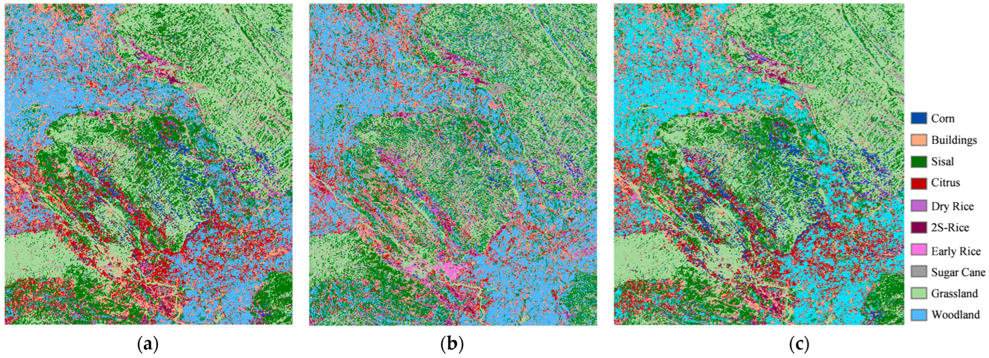
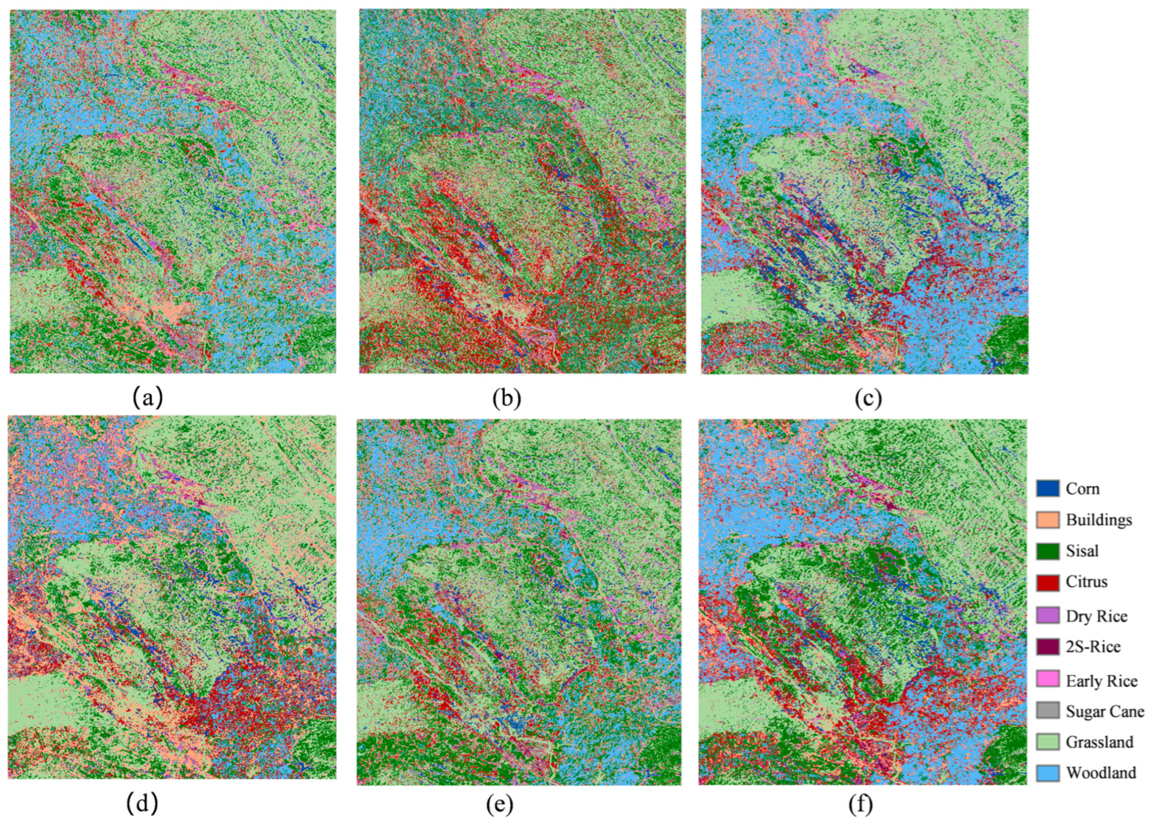
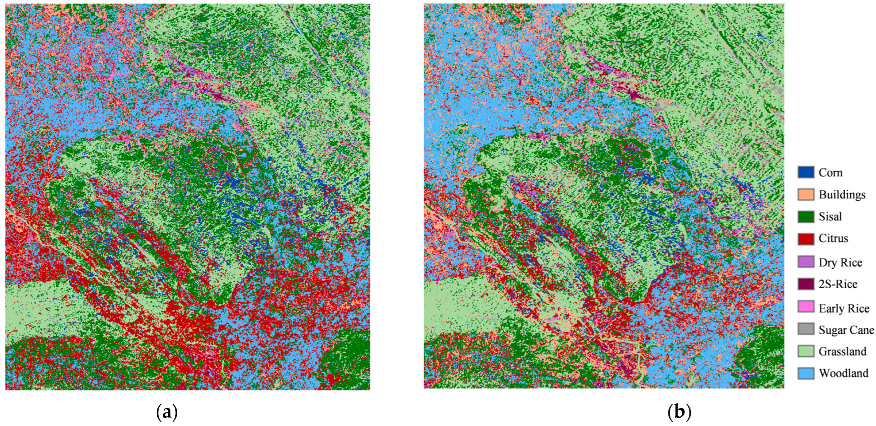
This study evaluates the efficacy of six distinct models in the crop classification task: CNN, LSTM, UNet, ViT, CNN-att, and our proposed model (DMoE-ViT), which utilizes long tail sample difficulty partitioning and the MOE mechanism. The results are presented in

Table 3. Classification results of study area 1.

Classes	CNN	LSTM	UNet	ViT	CNN-att	Ours
Corn	94.10%	94.30%	100.00%	99.20%	99.40%	100.00%
Buildings	56.80%	83.40%	74.80%	96.60%	96.20%	86.80%
Sisal	86.60%	88.50%	100.00%	98.30%	95.40%	100.00%
Citrus	93.30%	93.70%	100.00%	97.50%	98.90%	100.00%
Dry Rice	88.60%	93.90%	99.60%	91.80%	96.20%	96.50%
2S-Rice	86.00%	69.40%	0.00%	76.70%	86.70%	99.30%
Early Rice	78.30%	94.10%	100.00%	97.40%	96.90%	97.40%
Sugar Cane	96.60%	75.10%	99.60%	95.20%	92.50%	99.80%
Grassland	63.00%	65.80%	93.50%	83.40%	81.30%	89.30%
Woodland	99.80%	97.30%	100.00%	100.00%	99.80%	100.00%
OA	84.40%	85.79%	88.48%	93.92%	94.70%	96.40%
Recall	0.844	0.858	0.885	0.939	0.906	0.964
F1-score	0.841	0.855	0.851	0.938	0.944	0.964
Kappa	0.827	0.842	0.872	0.932	0.938	0.960

and Figure 9. Figure 9 illustrates the distribution map of crop types obtained using different classification methods in Study Area 1. Overall, the classification results are close to the ground truth labels, with only a small number of misclassifications and omissions. The proposed DMoE-ViT model preserves the boundaries of crop types as clearly as possible. Furthermore, Table 3 provides a quantitative evaluation of the five comparison models on the validation set. By comparing the classification accuracy, it can be found that our method outperforms the other five models in several key evaluation indices. Specifically, CNN shows some advantages in the aspect of underlying feature extraction. However, due to the lack of global information modeling, it performs poorly in handling complex categories and spatial structures, with an overall accuracy (OA) of 0.844 and an F1-score of 0.841. LSTM excels in sequence data processing, but due to its inability to effectively model spatial information, it achieves a lower accuracy in crop classification tasks, with an OA of 0.858 and an F1-score of 0.855. UNet performs well in image segmentation tasks, but its architecture does not effectively capture global information nor consider sample difficulty differences, resulting in lower accuracy in crop classification, with an OA of 0.885 and an F1-score of 0.851. ViT captures global information effectively through the self-attention mechanism; however, the lack of dynamic adjustment for sample difficulty leads to slightly poorer performance in complex tasks, with an OA of 0.939 and an F1-score of 0.938. The CNN-att model introduces an attention mechanism to enhance local feature learning but fails to address the issue of long tail sample difficulty differences, achieving an OA of 0.947 and an F1-score of 0.944. In contrast, our method, which combines sample difficulty partitioning and the MOE mechanism, dynamically adjusts the model’s weights, allowing it to optimize performance more effectively when handling samples of varying difficulty. Our model outperforms all other methods across all evaluation metrics, particularly in complex tasks and when handling high-difficulty samples. The OA of our model reaches 0.964, the Recall is 0.964, the F1-score is 0.964, and the Kappa is 0.960, demonstrating its significant advantage in crop classification tasks.

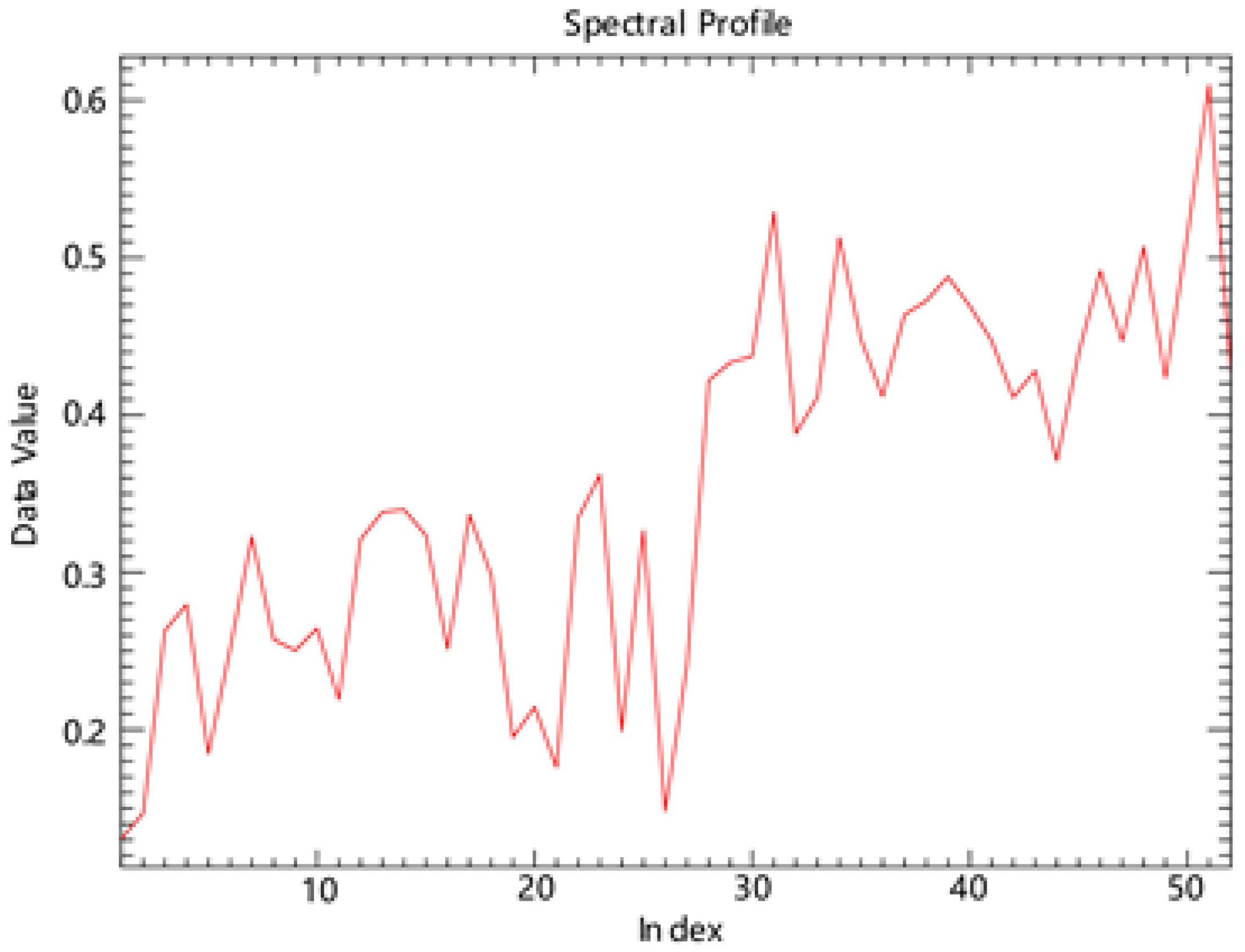
Observation of Table 3 reveals that the accuracy observed for the “Buildings” category is relatively low. Analysis indicates that this stems primarily from the inherent spatio-temporal complexity and fragmented characteristics of this category. Specifically, samples within this category exhibit pronounced spatial heterogeneity (encompassing diverse architectural styles, complex geometric contours, and urban-rural background variations), image fragmentation (resulting in blurred textures and indistinct boundaries due to low resolution or occlusion), and non-linear temporal fluctuations (manifesting as pronounced spectral variations influenced by seasonal changes, weather conditions, and acquisition timing). As illustrated in Figure 10, the spectral curves of buildings exhibit pronounced dynamic complexity; Figure 11 further elucidates their fragmented morphology and blurred textural characteristics. Within the MoE framework, despite three tiers of expert networks processing data by difficulty, conflicts in feature extraction (such as inconsistencies in texture versus geometry prioritisation) and challenges in integrating gated network outputs ultimately led to a marked decline in classification accuracy.

5.2.2. Results of Study Area 2

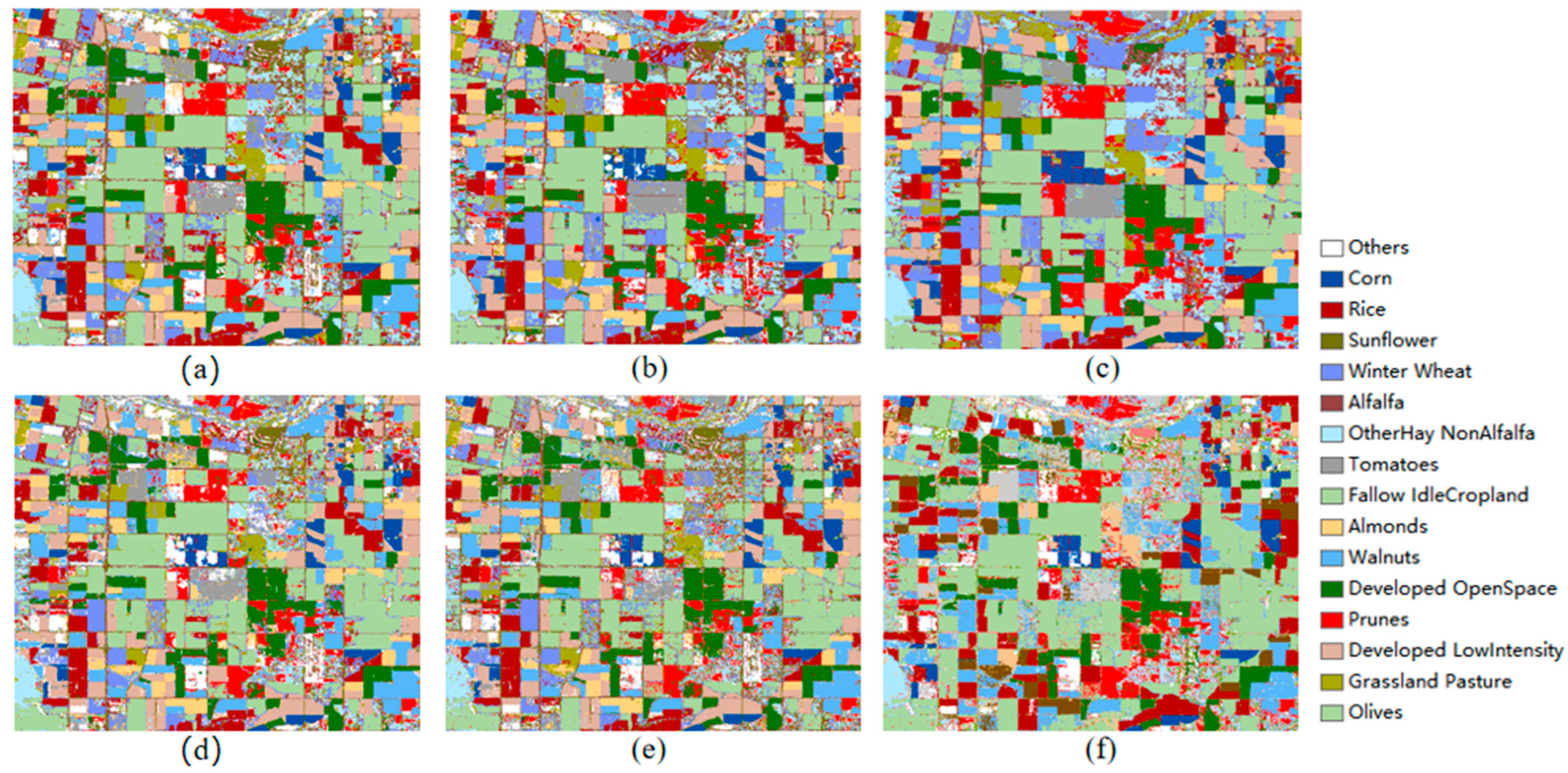
The experimental results of different classification methods in study area 2 are shown in Figure 12. Again, the prediction results of all methods are very similar to the labels, with only a small number of misclassified and missed pixels. Compared with our method, the predictions of other methods are affected by random noise, especially in non-uniformly closed areas. At the same time, our method retains the boundaries between farmland patches as clearly as possible, providing results that are closer to the actual crop distribution on the ground. To better evaluate the model’s ability to distinguish between different crops, the crop types in this area are more complex than those in the first study area.

Table 4. Classification results of study area 2.

Classes	CNN	LSTM	UNet	ViT	CNN-att	Ours
Others	39.70%	22.90%	0.00%	49.00%	45.60%	66.10%
Corn	94.20%	93.70%	95.90%	92.60%	93.90%	97.50%
Rice	74.40%	64.30%	66.90%	75.90%	76.60%	76.10%
Sunflower	49.70%	28.80%	0.00%	48.00%	54.30%	84.10%
Winter Wheat	47.50%	45.40%	53.90%	49.60%	48.5%%	81.70%
Alfalfa	63.00%	52.80%	81.60%	68.40%	60.50%	87.80%
OtherHay	67.20%	63.30%	75.10%	66.30%	62.70%	55.70%
Tomatoes	54.20%	45.40%	49.20%	68.80%	63.80%	84.80%
Fall-IdleCropland	94.50%	95.00%	95.50%	94.80%	94.10%	84.30%
Almonds	83.60%	81.80%	81.10%	88.20%	84.30%	57.90%
Walnuts	64.50%	63.50%	68.30%	67.90%	66.60%	67.30%
DevOpenSpace	72.10%	67.20%	74.40%	74.10%	74.00%	67.60%
Prunes	62.50%	55.30%	70.30%	68.30%	62.80%	53.40%
Dev-LowIntensity	85.80%	84.50%	88.20%	86.00%	84.40%	70.30%
Grassland pasture	49.80%	39.20%	48.60%	56.00%	56.20%	98.50%
Olives	63.30%	59.30%	67.70%	65.50%	65.10%	90.80%
OA	66.71%	60.25%	63.58%	65.50%	68.44%	79.20%
Recall	0.667	0.603	0.636	0.655	0.684	0.792
F1-score	0.668	0.602	0.599	0.657	0.684	0.791
Kappa	0.645	0.576	0.611	0.627	0.663	0.777

presents the classification results of the five models in study area 2 in quantitative terms. It can be seen that our model achieves the best overall accuracy (OA), Kappa coefficient, and F1-score among all methods.

The performance of the proposed difficulty-based MoE model was significantly influenced by landscape heterogeneity. As shown in Section 5.2.1, the model achieved its best performance in the highly fragmented Study Area 1 (Pingguo City). The complex class boundaries and abundant mixed pixels in this area generated training samples with a broad spectrum of difficulties, which aligned well with the model’s design principle of leveraging multiple experts to handle distinct difficulty subsets, thereby enabling the capture of subtle thematic variations. Conversely, in the homogeneous agricultural plains of Study Area 2 (Yolo Country), the simple landscape structure and uniform land-cover types resulted in a dataset with predominantly low and less-differentiated sample difficulties. This undermined the synergistic advantage of the multi-expert mechanism, thus limiting the model’s performance. Furthermore, the potential classification noise and spatial inaccuracies inherent in the CDL reference data for such homogeneous regions may have further compromised the training process and final accuracy.

5.2.3. Compared with the Latest Benchmark Method

To comprehensively evaluate the effectiveness of the proposed method, we benchmarked it against two representative state-of-the-art approaches in long tail visual recognition: TLC [47], which leverages evidence-theoretic uncertainty estimation and dynamic multi-expert selection, and BagofTricks-LT [48], which systematically integrates multiple high-efficiency training techniques. All experiments were conducted under identical train-test splits and evaluation metrics to ensure fair comparison. As shown in

Table 5. Overall performance comparison of three models.

Method	Accuracy	Recall	F1-score	Kappa
TLC	0.605	0.597	0.587	0.560
BagofTricks-LT	0.587	0.587	0.539	0.540
Ours	0.964	0.964	0.964	0.960

, our method significantly outperforms both baselines across all four core evaluation metrics. Specifically, our approach achieves accuracy improvements of 35.9% and 37.7% over TLC and BagofTricks-LT, respectively. Moreover, the substantial gains in F1-score and Kappa coefficient further indicate that our method not only excels in overall classification accuracy but also achieves superior balance in per-class predictive performance and consistency between predictions and ground-truth labels.

To further elucidate the sources of performance disparity, we analysed the limitations of the benchmark methods on our dataset. A detailed comparison of per-class classification accuracy is presented in

Table 6. Accuracy Comparison Across Categories on Three Models.

Classes	BagofTricks-LT	TLC	Ours
Corn	0.8253	0.778	1.00
Buildings	0.6430	0.601	0.868
Sisal	0.8200	0.671	1.00
Citrus	0.9944	0.716	1.00
Dry Rice	0.0388	0.510	0.9650
2S-Rice	0.0952	0.184	0.9930
Early Rice	0.0986	0.667	0.9740
Sugarcane	0.9216	0.552	0.9980
Grassland	0.3499	0.430	0.8930
Woodland	0.9288	0.861	1.0000

, which clearly reveals the failure modes of the competing approaches while highlighting the strengths of our method. As shown in Table 6, our approach achieves superior performance in two primary aspects. First, the uncertainty-weighted fusion mechanism demonstrates robust adaptability by automatically identifying and down-weighting unreliable predictions. This capability proves particularly valuable when handling crop samples with phenotypically similar traits but divergent growth conditions, effectively mitigating overconfident, erroneous decisions. Second, the specialised feature learning paradigm plays a pivotal role in performance gains: each ViT expert is independently trained to develop optimal representations tailored to its designated difficulty tier. This stands in stark contrast to TLC’s shared backbone architecture and substantially enhances our model’s discriminative and modelling capacity for challenging samples. Through these comprehensive and in-depth comparative experiments and analyses, we conclusively demonstrate that the proposed method not only achieves full comparability with current state-of-the-art techniques but also attains substantial performance superiority.

Although TLC exhibits a theoretically robust design, it reveals several critical limitations in the context of our specific application scenario. First, its reliance on Dempster–Shafer evidence theory leads to bias propagation in uncertainty estimation under long tail distributions. Subtle feature differences between certain classes (e.g., Dry Rice and 2S-rice), compounded by inconsistent growth environments, result in systematic biases in uncertainty quantification. These biases subsequently disrupt the expert selection process, forming erroneous feedback loops. Second, the dynamic expert selection mechanism largely fails on our dataset, as it struggles to accurately identify samples requiring specialized handling due to low inter-class discriminability. This is corroborated by Table 6, which shows consistently low accuracy of TLC on Rice-related categories. Finally, TLC’s feature representation capacity is constrained: its multi-expert modules share a common backbone network, preventing individual experts from developing specialized representations tailored to different difficulty levels, thereby impairing discriminative performance on hard samples.

As a general-purpose ensemble of techniques optimized for broad applicability, BagofTricks-LT exhibits apparent limitations when applied to the specific long tail distribution in this study. These shortcomings manifest in two primary aspects. First, the technique combination, optimised on generic datasets, proves suboptimal for our domain-specific data distribution. Specifically, when addressing homologous crop variants arising from differences in growth conditions and phenological stages (e.g., Dry Rice, 2S-Rice, and Early Rice), its resampling and reweighting strategies fail to capture subtle inter-class distinctions, resulting in extremely low recognition accuracy on certain classes (some below 0.1%) and severely constraining overall performance. Second, the method lacks explicit modeling of sample difficulty, precluding difficulty-aware differential treatment. Consequently, it performs poorly on structurally hard samples in our dataset—for instance, achieving only 3.88% accuracy on the Dry Rice class (see Table 6)—further highlighting its deficiency in difficulty perception.

6. Discussion

6.1. Multiple Experts’ Output Results for a Single Sample

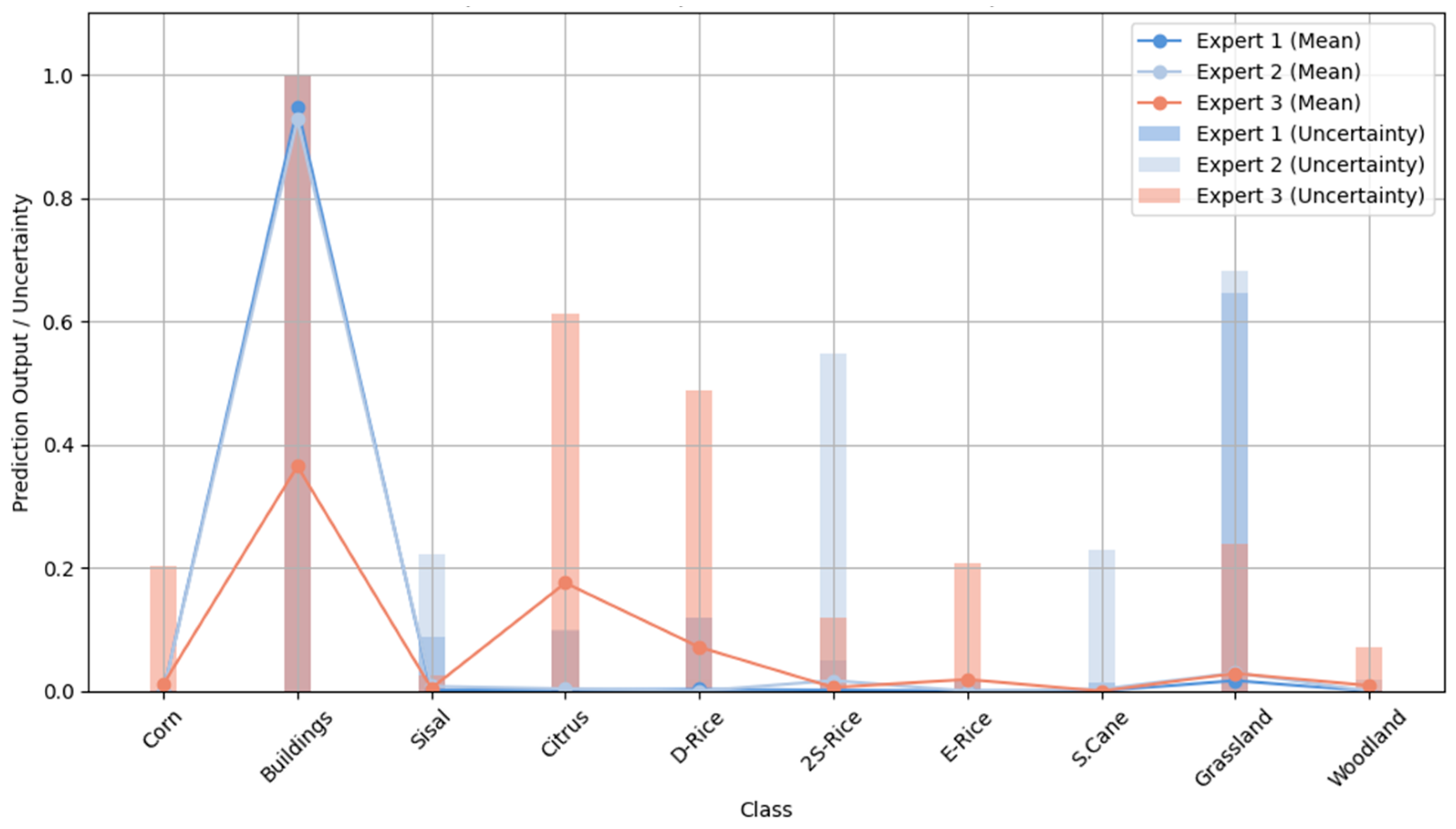
In Figure 13, we can intuitively observe the performance differences of the Mixture of Experts model on a single sample. Specifically, simple samples usually exhibit lower uncertainty because the model’s predictions on these samples are more consistent, and their features are typically more straightforward to distinguish, enabling the model to make rapid and accurate decisions. For example, in a simple image classification task, all expert networks tend to provide similar outputs when processing these samples, resulting in more credible final weighted predictions, thereby reducing uncertainty values. In contrast, hard samples exhibit higher uncertainty, suggesting that the model’s predictions for these samples are less credible. These samples typically exhibit more complex features, blurred boundaries, contain noise, and may be influenced by factors such as varying backgrounds, occlusions, or similar categories. Therefore, different expert networks will produce different predictions when processing these samples.

6.2. The Impact of Long Tail Sample Difficulty Classification on Experimental Results

In this study, we compared the effects of distinguishing between long tail sample difficulty and not distinguishing between long tail sample difficulty on crop classification models, as shown in Figure 14 and Figure 15 and

Table 7. Crop classification accuracy table without distinguishing long tail sample difficulty. The classification results are compared under two conditions: one that accounts for sample long tail difficulty and the other that disregards long tail sample difficulty.

Classes	No Consideration of Long Tail Sample Difficulty	Consideration of Long Tail Sample Difficulty
Corn	99.20%	100.00%
Buildings	96.60%	86.80%
Sisal	98.30%	100.00%
Citrus	97.50%	100.00%
Dry Rice	91.80%	96.50%
Double-season Rice	76.70%	99.30%
Early Rice	97.40%	97.40%
Sugar Cane	95.20%	99.80%
Grassland	83.40%	89.30%
Woodland	100.00%	100.00%
OA	93.92%	96.40%
Recall	0.939	0.964
F1-score	0.938	0.964
Kappa	0.932	0.960

. Through the analysis of the experimental results, we found that the classification accuracy was significantly improved by classifying samples according to their difficulty, especially for high-difficulty samples. First, in an experiment that does not distinguish the difficulty of samples, all types of samples, including easy, moderate, and hard samples, are input to each expert network. Due to the complexity and indistinguishable features of difficult-to-classify samples, this method of inputting samples poses challenges for the model to effectively learn the features of these samples, resulting in low recognition accuracy of difficult-to-classify types such as grassland and double-cropping rice.

In contrast, in the experiment to distinguish the difficulty of samples, a better recognition effect was achieved by inputting samples of different difficulty levels into the expert network. Specifically, Expert 1 handles all samples (including easy and moderate samples), Expert 2 handles moderate and hard samples, and Expert 3 handles only hard samples. This approach enables each expert network to focus on learning the features of a particular hard sample, allowing the model to more precisely capture and optimize the features of these samples, thereby improving the recognition of those samples. Specifically, experiments that distinguish sample difficulty have significantly improved accuracy for high-difficulty categories. For example, the accuracy of the grass category improved from 83.4% to 89.3%, a 5.9% increase. The accuracy rate of double-cropping rice increased from 76.7% to 99.3%, representing a 22.6% improvement. This demonstrates that the model can effectively enhance the recognition performance of challenging samples by accurately assessing their difficulty.

On the other hand, for categories that are relatively easy to classify, such as sisal, woodland, and citrus, there was little change in accuracy, suggesting that the difficulty of distinguishing samples has little effect on these easier categories. At the same time, it also indicates that the difference in sample difficulty has a minimal impact on the classification results for low-difficulty categories. In summary, by comparing the results of the two experiments, we can conclude that the classification accuracy of high-difficulty samples is significantly improved by the difficulty of distinguishing them, especially for categories with high classification difficulty. For simpler classes, the effect of sample difficulty on model performance is relatively small. Therefore, the method of distinguishing sample difficulty has obvious advantages in improving classification accuracy, especially for complex tasks and high-difficulty samples.

6.3. The Relative Contribution and Significance of Optical and Radar Signatures

To quantitatively evaluate the contribution of each modality in the crop classification task, we designed a systematic ablation study. Under the controlled-variable approach, with a fixed model architecture, hyperparameters, and training data, we constructed seven data configurations, ranging from single-modality to full-modality combinations (NDVI-only, VV-only, VH-only, NDVI + VV, NDVI + VH, VV + VH, and NDVI + VV + VH), to compare classification performance across different modal inputs comprehensively. The evaluation framework integrates four dimensions: overall accuracy, marginal gain, category dominance, and relative contribution index. Specifically, we first assessed overall performance using overall accuracy. Subsequently, we calculated the marginal gain from each modality in combined scenarios, counted the frequency with which each modality achieved the highest F1-score across different crop categories, and finally synthesized these metrics through weighted normalization to generate a relative contribution index. This process establishes an evident modality importance ranking, providing a quantitative basis for optimising multimodal remote sensing data fusion strategies.

6.3.1. Heatmap of the Importance of Each Modal to Category

Table 8. Heatmap of the importance of modes for categories.

Class	NDVI	VV	VH	Dominant Mode
Corn	○ (9.37)	□ (0.19)	○ (6.12)	NDVI
Buildings	▼ (−1.73)	▲ (37.47)	☆ (16.63)	VV
Sisal	□ (1.72)	☆ (26.05)	○ (6.70)	VV
Citrus	☆ (17.05)	□ (1.92)	□ (0.00)	NDVI
Dry Rice	□ (4.16)	○ (5.07)	☆ (25.62)	VH
2S-Rice	☆ (28.18)	▲ (55.85)	○ (7.07)	VV
Early Rice	▼ (−0.86)	▲ (71.47)	☆ (17.66)	VV
Sugar Cane	□ (3.24)	▲ (61.18)	▲ (31.54)	VV
Grassland	□ (4.60)	☆ (15.69)	☆ (27.73)	VH
Woodland	○ (7.25)	□ (0.57)	□ (0.38)	NDVI

utilizes a symbolic heatmap to visually illustrate the local importance of the three modalities—NDVI, VV, and VH—across various land cover categories. The symbolic representation is defined as follows: ▲ (> 30%) denotes very high importance, ☆ (15%–30%) indicates high significance, ○ (5%–15%) represents moderate importance, □ (0%–5%) signifies low relevance, and ▼ (< 0%) designates a negative contribution. The results demonstrate that VV polarisation assumes an absolutely dominant role for several crop types, including early rice (▲), sugarcane (▲), and double-cropping rice (▲). VH polarisation provides substantial textural enhancement for sugarcane (▲), grassland (☆), and dryland-to-paddy conversion (☆). NDVI exhibits specialised utility in categories associated with vegetation health, such as citrus (☆), corn (○), and woodland (○). Simultaneously, the analysis reveals distinct inter-modal interactions: NDVI exhibits a negative impact (▼) on building and early rice identification, while VH contributes minimally (□) for citrus, bordering on redundancy. These patterns highlight the existence of both complementary and conflicting mechanisms among the different modalities.

The local contribution value of each mode to a specific category within the table is defined as:

$${\mathit{C}\mathit{o}\mathit{n}\mathit{t}\mathit{r}\mathit{i}\mathit{b}\mathit{u}\mathit{t}\mathit{i}\mathit{o}\mathit{n}}_{\mathit{X}\to \mathit{Y}}={\mathit{P}}_{\mathit{Y}}\left(\mathit{N}\mathit{D}\mathit{V}\mathit{I}+\mathit{V}\mathit{V}+\mathit{V}\mathit{H}\right)-{\mathit{P}}_{\mathit{Y}}\left(\mathit{M}\backslash \left\{\mathit{X}\right\}\right)$$

(21)

Among the various accuracy metrics, ${\mathit{P}}_{\mathit{Y}}$ denotes the classification accuracy for category Y, while $\mathbf{M}\backslash \left\{\mathbf{X}\right\}$ represents the combination of the other two modalities, excluding modality X.

6.3.2. Global Modality Contribution Ranking

Through a comprehensive analysis of Table 8 and

Table 9. Ranking of Modal Global Contributions.

Combination Method	Overall Contribution (Accuracy Improvement)	Number of Locally Dominant Classes	Ratio (%)	Ranking
VV	+25.98% (NDVI + VH → NDVI + VV + VH)	5 (Early Rice, Sugar Cane, 2S-Rice, Sisal, Buildings)	46.39	1
VH	+13.59% (NDVI + VV → NDVI + VV + VH)	3 (Sugar Cane, Grassland, Dry Rice)	24.26	2
NDVI	+6.48% (VV + VH → NDVI + VV + VH)	3(Citrus, Corn, Grassland)	3.24	3

, it is clear that VV dominates the highest number of land cover categories, followed by VH and NDVI. By further classifying these dominant categories based on their characteristic attributes, a distinct pattern of modality-specific strengths emerges: VV assumes a globally dominant role, VH exhibits texture-discrimination dominance, while NDVI demonstrates a vegetation-oriented advantage. The quantitative results from the Ratio metric in Table 9 show that VV has the highest proportion, consistent with its top Ranking in the relative contribution index. VH ranks second, and NDVI third. These findings not only confirm the core driving role of VV in the overall classification performance but also further elucidate the complementary nature and hierarchical importance of the three modalities in specific discrimination tasks. This provides a solid quantitative foundation for optimising the design of multimodal fusion strategies.

The Overall Contribution value within each combination in the table is defined as:

$${\mathit{C}\mathit{o}\mathit{n}\mathit{t}\mathit{r}\mathit{i}\mathit{b}\mathit{u}\mathit{t}\mathit{i}\mathit{o}\mathit{n}}_{\mathit{X}\to \mathit{Y}}={{\mathit{P}}^{\mathit{\text{'}}}}_{\mathit{Y}}\left(\mathit{N}\mathit{D}\mathit{V}\mathit{I}+\mathit{V}\mathit{V}+\mathit{V}\mathit{H}\right)-{{\mathit{P}}^{\mathit{\text{'}}}}_{\mathit{Y}}\left(\mathit{M}\backslash \left\{\mathit{X}\right\}\right)$$

(22)

Within the Accuracy section, ${\mathit{P}\mathit{\text{'}}}_{\mathit{Y}}$ denotes the classification accuracy for category Y, while $\mathit{M}\backslash \left\{\mathit{X}\right\}$ represents the combination of the other two modalities excluding modality X. The column labelled Ranking indicates the importance ranking of each modality. In contrast, the column labeled “Ratio” shows the contribution ratio per scene—specifically, the proportion of Overall Contribution relative to the total number of all modality images.

6.4. Graded-Difficulty Proportionate Melting Experiment

To systematically validate the effectiveness of the proposed 3:2:1 difficulty stratification strategy, this section was designed to conduct comprehensive ablation experiments targeting the allocation ratios across three difficulty levels (Easy, Moderate, Hard). On the validation set of the first study area, the following four stratification configurations were evaluated:

• Uniform Distribution (1:1:1): Each difficulty level accounts for 33.3% as the baseline;
• Easy-Focused (4:2:1): Prioritizes foundational feature learning (Easy 57.1%, Moderate 28.6%, Hard 14.3%);
• Moderate-Difficulty Emphasis (2:2:1): Prioritizes learning complex patterns (Easy 40%, Moderate 40%, Hard 20%);
• Proposed Strategy (3:2:1): Gradual curriculum learning (Easy 50%, Moderate 33.3%, Hard 16.7%).

The experimental results are shown in

Table 10. Performance Comparison of Different Stratification Strategies in Crop Classification Tasks.

Layered Strategy	Accuracy	Recall	F1-Score	Kappa	OA	Training Stability/Epoch
1:1:1	0.903	0.909	0.908	0.896	0.909	42
2:2:1	0.916	0.924	0.916	0.913	0.924	39
4:2:1	0.948	0.955	0.954	0.947	0.955	35
3:2:1	0.964	0.964	0.964	0.960	0.964	30

. Key evaluation metrics include overall classification accuracy (OA), Kappa coefficient, F1-score for hard samples, and training convergence speed (the number of iterations required to reach 95% of the final OA).

Table 10 presents comparative experimental results on a typical agricultural remote sensing dataset, demonstrating that the proposed 3:2:1 strategy achieves the best overall accuracy (OA), F1-score, and Kappa coefficient. Specifically, the OA of the proposed strategy is 5.5% higher than that of the 1:1:1 baseline, with improved convergence stability and fewer required training epochs. Further analysis reveals that the 1:1:1 strategy leads to premature and excessive exposure to hard samples, which hinders the stable learning of fundamental discriminative features. The 4:2:1 strategy results in insufficient training of hard samples, causing underfitting in the corresponding expert network. Meanwhile, the 2:2:1 strategy undermines the foundational role of easy samples, resulting in instability in overall feature learning. In contrast, the 3:2:1 strategy strikes an optimal balance between consolidating basic features and tackling challenging cases, thereby validating the rationality of its design.

This study constructs a Mixture-of-Experts (MoE) network that shares a core conceptual resonance with recent advanced multi-scale attention frameworks. For instance, in the task of lithological unit classification in vegetated areas, Hui et al. [49] introduced Multi-Scale Enhanced Cross-Attention (MSECA) and Wavelet-Enhanced Cross-Attention (WCCA) to strengthen the model’s ability to capture both fine-grained local details and long-range contextual dependencies. The MoE design in this work can be viewed as a corresponding, yet more generalized, “model capacity allocation” mechanism: The expert networks handling simple samples function similarly to MSECA, focusing on extracting robust local features from clear and common patterns. The expert networks handling challenging samples emulate the role of WCCA, aiming to model the broader contextual information required for complex and sparse samples.

6.5. Stratified Statistical Analysis on Samples of Varying Difficulty Levels

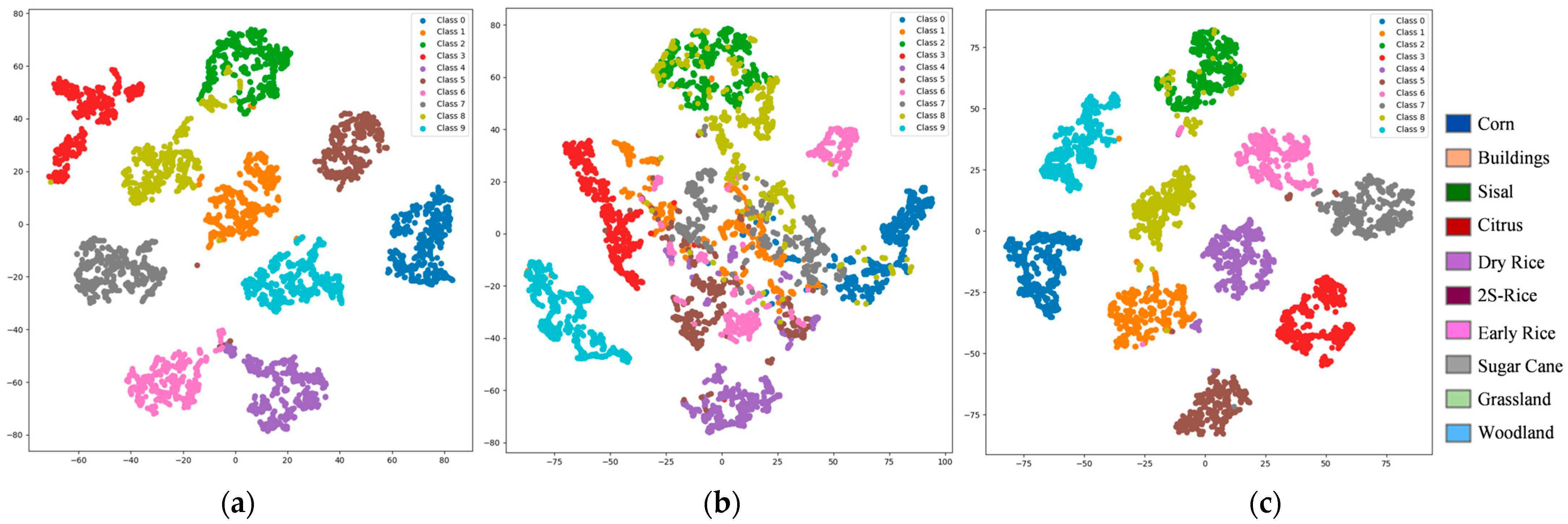
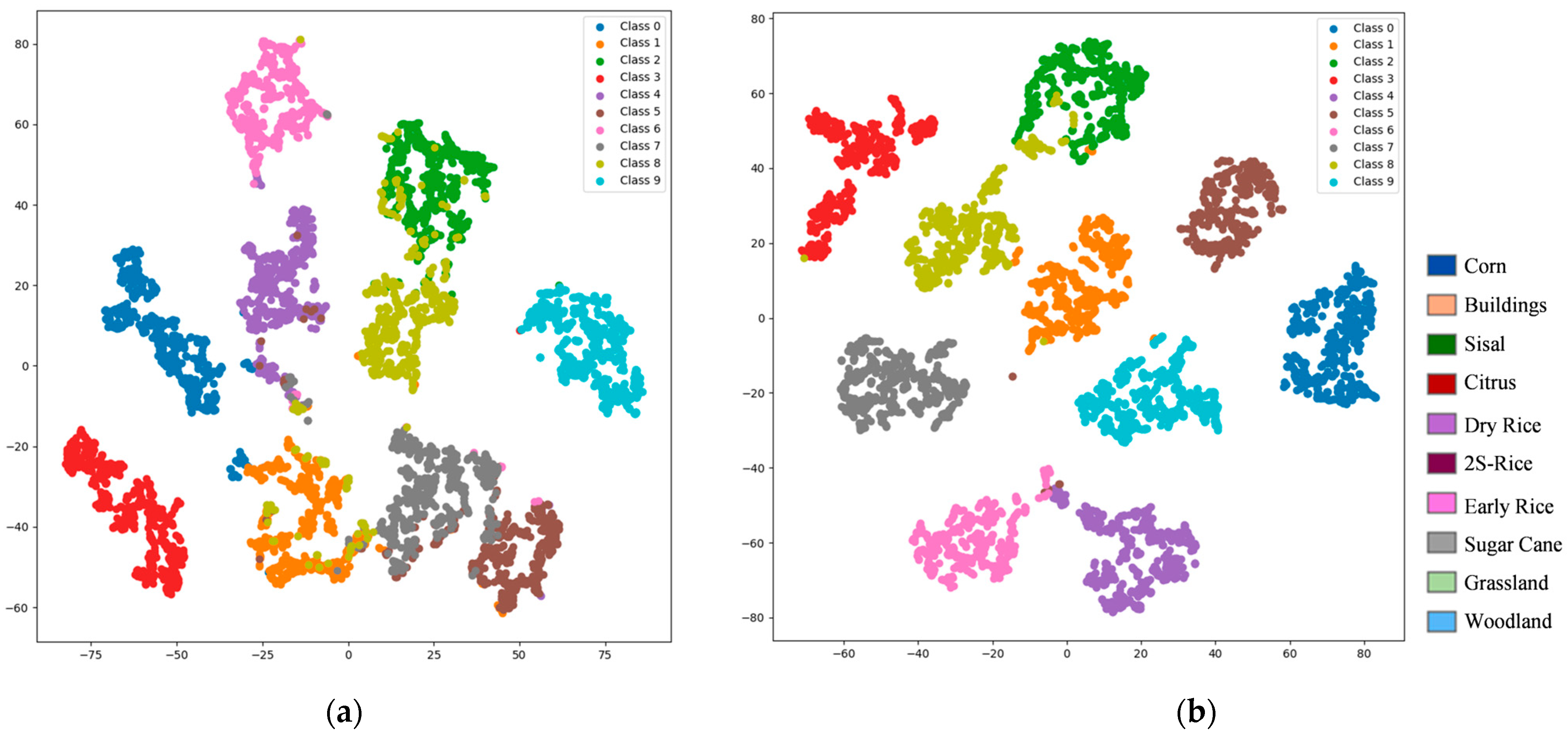
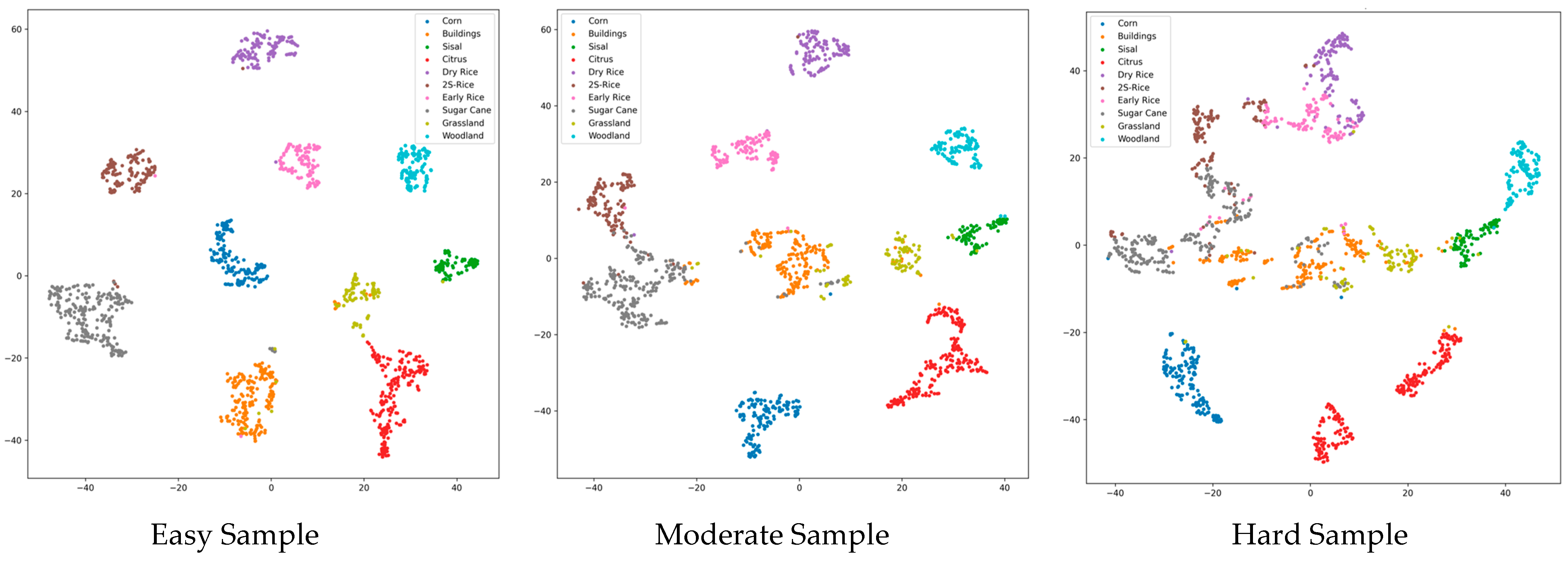
To rigorously validate the efficacy of the difficulty-aware mechanism and to enable fine-grained evaluation within each difficulty stratum, we establish independent assessment frameworks for the three difficulty levels (easy, moderate, and hard), reporting Accuracy, Recall, F1-score, Kappa, and Overall Accuracy (OA) for each subset, along with per-class precision.

Table 11. Overall Performance Comparison of Different Difficulty Subsets.

Sample	Accuracy	Recall	F1-score	Kappa	OA
Easy Sample	0.978	0.977	0.978	0.975	0.978
Moderate Sample	0.916	0.915	0.914	0.905	0.916
Hard Sample	0.736	0.735	0.726	0.699	0.736

presents the complete stratified results,

Table 12. Stratified Accuracy by Category (%).

Classes	Easy Sample	Moderate Sample	Hard Sample
Corn	100.0	100.0	99.31
Buildings	97.83	88.04	67.93
Sisal	100.0	97.40	89.61
Citrus	100.0	100.0	100.0
Dry Rice	99.17	94.17	62.50
2S-Rice	96.77	75.00	17.74
Early Rice	98.21	95.54	48.21
Sugar-Rice	97.38	94.76	82.10
Grassland	85.11	61.70	61.70
Woodland	100.0	98.04	82.35

details the per-class stratified accuracies, Figure 16 illustrates the confusion matrices for the different difficulty subsets, and Figure 17 depicts the t-SNE visualisations of the respective difficulty subsets.

The results in Table 11 demonstrate a natural performance degradation with increasing difficulty (Easy > Moderate > Hard), fully aligning with the anticipated distribution. Our approach achieves an overall OA of 0.964, attaining or approaching the optimal single-expert performance across all subsets, thereby highlighting the MoE framework’s success in synergistically integrating specialised capabilities for distinct difficulty strata.

Table 12 further reveals that head categories (Corn, Citrus, Sisal, Woodland) approach or reach 100% in the Easy and Moderate subsets, with our method maintaining 100.0% throughout, indicating efficient, lossless processing of simple samples and high inter-crop discriminability in Figure 16 and Figure 17. Tail-end challenging categories markedly benefit from expert collaboration; for instance, 2S-Rice surges from 17.74% to 96.77% in the Difficult subset, attributable to Expert-3’s deep modelling of complex spectral features. Similarly, Early Rice (48.21% → 98.21%), Dry Rice (62.50% → 99.17%), Buildings (67.93% → 97.83%), and Grassland (61.70% → 85.11%) achieve dramatic improvements, underscoring the combined contributions of Expert-2 and Expert-3. These categories, characterized by high entropy due to seasonal variations, cropping patterns, or land-cover confusion, represent prototypical long tail complex cases. Although the Difficult subset averages ~70% in isolation, our method—through dynamic weighted fusion via the gating network and uncertainty calibration—transforms potential performance drags into global gains, yielding an ultimate overall OA of 96.4%.

7. Conclusions

In this paper, a Difficulty-based Mixture of Experts Vision Transformer framework (DMoE-ViT) is proposed for accurate crop type mapping. This framework utilizes the Vision Transformer (ViT) architecture and a Mixture of Experts model (MoE) gating mechanism to handle samples of varying difficulty levels in a multi-expert model. Long tail samples were categorized into three difficulty levels—easy, moderate, and hard—and split into three datasets. Each dataset was fed into separate ViT networks, generating distinct output results. The DMoE-ViT model computed appropriate weights for each dataset based on its difficulty level. During testing, the same data samples and their labels were passed through the three networks, and the predictions were weighted according to the model and aggregated to produce the final output.

Additionally, uncertainty was calculated for the final prediction, with an output weight assigned based on this uncertainty, which was then multiplied by the aggregated result to yield the final prediction. Our experimental results demonstrate that this approach enhances the model’s performance by incorporating a sample difficulty classification mechanism, enabling the model to adjust its learning process according to the complexity of the long tail samples. The implementation of the MoE gating mechanism enhances the efficiency of processing diverse sample types and improves the stability and accuracy of models across many categories. This method can provide a better understanding of the relationship between sample complexity and model performance when dealing with hard samples, highlighting the importance of introducing difficulty perception strategies in training deep learning models. Future endeavours may boost the model’s performance through various improvements. The precision of classification can be enhanced by refining the difficulty classification process using methods such as clustering algorithms, deep learning-based feature extraction, or domain-specific expertise.

Additionally, adjusting the sample classification threshold can more accurately distinguish between different difficulty levels. Second, model flexibility and performance can be improved by exploring alternative expert architectures, such as CNNS, RNNS, or hybrid models. Finally, the robustness of the model to different sample complexities can also be improved by integrating uncertainty quantification or data enhancement strategies.

References

1. Horrigan, L.; Lawrence, R.S.; Walker, P. How sustainable agriculture can address the environmental and human health harms of industrial agriculture. Environ. Health Perspect. 2002, 110, 445–456. [Google Scholar] [PubMed]
2. Arias, M.; Campo-Bescós, M.Á.; Álvarez-Mozos, J. Crop Classification Based on Temporal Signatures of Sentinel-1 Observations over Navarre Province, Spain. Remote Sens. 2020, 12, 278. [Google Scholar] [CrossRef]
3. Bargiel, D. A new method for crop classification combining time series of radar images and crop phenology information. Remote Sens. Environ. 2017, 198, 369–383. [Google Scholar] [CrossRef]
4. Wolfe, D.W.; Degaetano, A.T.; Peck, G.M.; Carey, M.; Ziska, L.H.; Leacox, J.; Kemanian, A.R.; Hoffmann, M.P.; Hollinger, D.Y.; Oppenheimer, M. Unique challenges and opportunities for northeastern US crop production in a changing climate. Clim. Change 2018, 146, 231–245. [Google Scholar] [CrossRef]
5. Wei, S.; Zhang, H.; Wang, C.; Wang, Y.; Xu, L. Multi-Temporal SAR Data Large-Scale Crop Mapping Based on U-Net Model. Remote Sens. 2019, 11, 68. [Google Scholar] [CrossRef]
6. Löw, F.; Duveiller, G. Defining the Spatial Resolution Requirements for Crop Identification Using Optical Remote Sensing. Remote Sens. 2014, 6, 9034–9063. [Google Scholar] [CrossRef]
7. Wang, H.; Ye, Z.; Wang, Y.; Liu, X.; Zhang, X.; Zhao, Y.; Li, S.; Liu, Z.; Zhang, X. Improving the crop classification performance by unlabeled remote sensing data. Expert Syst. Appl. 2024, 236, 121283. [Google Scholar] [CrossRef]
8. Liu, J.; Feng, Q.; Gong, J.; Zhou, J.; Liang, J.; Li, Y. Winter wheat mapping using a random forest classifier combined with multi-temporal and multi-sensor data. Int. J. Digit. Earth 2018, 11, 783–802. [Google Scholar] [CrossRef]
9. Saini, R.; Ghosh, S.K. Crop Classification on Single Date Sentinel-2 Imagery Using Random Forest and Suppor Vector Machine. ISPRS Int. Arch. Photogramm. Remote Sens. Spat. Inf. Sci. 2018, 42, 683–688. [Google Scholar] [CrossRef]
10. Loew, F.; Michel, U.; Dech, S.; Conrad, C. Impact of feature selection on the accuracy and spatial uncertainty of per-field crop classification using Support Vector Machines. ISPRS J. Photogramm. Remote Sens. 2013, 85, 102–119. [Google Scholar]
11. MorenoRevelo, M.Y.; Guachiguachi, L.; Gómez-Mendoza, J.B.; Revelo-Fuelagan, J.; Peluffo-Ordóñez, D.H. Enhanced Convolutional-Neural-Network Architecture for Crop Classification. Appl. Sci. 2021, 11, 4292. [Google Scholar] [CrossRef]
12. Liu, M.; He, W.; Zhang, H. WPS:A whole phenology-based spectral feature selection method for mapping winter crop from time-series images. ISPRS J. Photogramm. Remote Sens. 2024, 210, 141–159. [Google Scholar] [CrossRef]
13. Msangameno, D.J.; Mangora, M.M. Aspects of Seasonal and Long-term Trends in Fisheries and Livelihoods in the Kilombero River Basin, Tanzania. Afr. J. Trop. Hydrobiol. Fish. 2016, 14, 1–11. [Google Scholar]
14. Sousa, D.; Small, C. Mapping and Monitoring Rice Agriculture with Multisensor Temporal Mixture Models. Remote Sens. 2019, 11, 181. [Google Scholar] [CrossRef]
15. Crisóstomo de Castro Filho, H.; Abílio de Carvalho Júnior, O.; Ferreira de Carvalho, O.L.; Pozzobon de Bem, P.; dos Santos de Moura, R.; Olino de Albuquerque, A.; Rosa Silva, C.; Guimaraes Ferreira, P.H.; Fontes Guimarães, R.; Trancoso Gomes, R.A. Rice Crop Detection Using LSTM, Bi-LSTM, and Machine Learning Models from Sentinel-1 Time Series. Remote Sens. 2020, 12, 2655. [Google Scholar] [CrossRef]
16. Li, Z.; Chen, G.; Zhang, T. A CNN-Transformer Hybrid Approach for Crop Classification Using Multitemporal Multisensor Images. IEEE J. Sel. Top. Appl. Earth Obs. Remote Sens. 2020, 13, 847–858. [Google Scholar] [CrossRef]
17. Wang, R.; Ma, L.; He, G.; Johnson, B.A.; Yan, Z.; Chang, M.; Liang, Y. Transformers for remote sensing: A systematic review and analysis. Sensors 2024, 24, 3495. [Google Scholar] [CrossRef] [PubMed]
18. Aleissaee, A.A.; Kumar, A.; Anwer, R.M.; Khan, S.; Cholakkal, H.; Xia, G.-S.; Khan, F.S. Transformers in remote sensing: A survey. Remote Sens. 2023, 15, 1860. [Google Scholar] [CrossRef]
19. Firbank, L.G. Short-term variability of plant populations within a regularly disturbed habitat. Oecologia 1993, 94, 351–355. [Google Scholar] [CrossRef]
20. Xue, Z.; Du, P.; Feng, L. Phenology-Driven Land Cover Classification and Trend Analysis Based on Long-term Remote Sensing Image Series. IEEE J. Sel. Top. Appl. Earth Obs. Remote Sens. 2014, 7, 1142–1156. [Google Scholar] [CrossRef]
21. Zhong, L.; Hu, L.; Zhou, H. Deep learning based multi-temporal crop classification. Remote Sens. Environ. 2019, 221, 430–443. [Google Scholar] [CrossRef]
22. Mazzia, V.; Khaliq, A.; Chiaberge, M. Improvement in Land Cover and Crop Classification based on Temporal Features Learning from Sentinel-2 Data Using Recurrent-Convolutional Neural Network (R-CNN). Appl. Sci. 2019, 10, 238. [Google Scholar] [CrossRef]
23. Hixson, M.; Scholz, D.; Fuhs, N.; Akiyama, T. Evaluation of several schemes for classification of remotely sensed data. Photogramm. Eng. Remote Sens. 1980, 46, 1547–1553. [Google Scholar]
24. Larsen, E.J. Introduction to Remote Sensing, 3rd ed.; Guilford Press: New York, NY, USA, 2002. [Google Scholar]
25. Wardlow, B.D.; Egbert, S.L.; Kastens, J.H. Analysis of time-series MODIS 250 m vegetation index data for crop classification in the U.S. Central Great Plains. Remote Sens. Environ. 2007, 108, 290–310. [Google Scholar] [CrossRef]
26. Yang, X.; Lo, C.P. Using a time series of satellite imagery to detect land use and land cover changes in the Atlanta, Georgia metropolitan area. Int. J. Remote Sens. 2002, 23, 1775–1798. [Google Scholar] [CrossRef]
27. Yang, Y.; Tao, B.; Ren, W.; Zourarakis, D.P.; Masri, B.E.; Sun, Z.; Tian, Q. An Improved Approach Considering Intraclass Variability for Mapping Winter Wheat Using Multitemporal MODIS EVI Images. Remote Sens. 2019, 11, 1191. [Google Scholar] [CrossRef]
28. Lunetta, R.S.; Shao, Y.; Ediriwickrema, J.; Lyon, J.G. Monitoring agricultural cropping patterns across the Laurentian Great Lakes Basin using MODIS-NDVI data. Int. J. Appl. Earth Obs. Geoinf. 2010, 12, 81–88. [Google Scholar] [CrossRef]
29. Qiu, B.; Luo, Y.; Tang, Z.; Chen, C.; Lu, D.; Huang, H.; Chen, Y.; Chen, N.; Xu, W. Winter wheat mapping combining variations before and after estimated heading dates. ISPRS J. Photogramm. Remote Sens. 2017, 123, 35–46. [Google Scholar] [CrossRef]
30. Liu, T.; Zhang, C.; Li, D. Reducing Overfitting In Deep Neural Networks By Intra-class Decorrelation. In Proceedings of the 2023 International Seminar on Computer Science and Engineering Technology (SCSET), New York, NY, USA, 29–30 April 2023; pp. 200–203. [Google Scholar]
31. Liu, Z.; Wei, P.; Wei, Z.; Yu, B.; Jiang, J.; Cao, W.; Bian, J.; Chang, Y. Handling inter-class and intra-class imbalance in class-imbalanced learning. arXiv 2021, arXiv:2111.12791. [Google Scholar]
32. Li, Z.; Kamnitsas, K.; Glocker, B. Analyzing overfitting under class imbalance in neural networks for image segmentation. IEEE Trans. Med. Imaging 2020, 40, 1065–1077. [Google Scholar] [CrossRef] [PubMed]
33. Wang, H.; Huang, Y.; Huang, H.; Wang, Y.; Li, J.; Gui, G. Uncertainty-Aware Dynamic Fusion Network with Criss-Cross Attention for multimodal remote sensing land cover classification. Inf. Fusion 2025, 123, 103249. [Google Scholar] [CrossRef]
34. Li, J.; He, W.; Li, Z.; Guo, Y.; Zhang, H. Overcoming the uncertainty challenges in detecting building changes from remote sensing images. ISPRS J. Photogramm. Remote Sens. 2025, 220, 1–17. [Google Scholar] [CrossRef]
35. Rey, M.; Mnih, A.; Neumann, M.; Overlan, M.; Purves, D. Uncertainty evaluation of segmentation models for Earth observation. arXiv 2025, arXiv:2510.19586. [Google Scholar] [CrossRef]
36. Sun, H.; Xu, A.; Lin, H.; Zhang, L.; Mei, Y. Winter wheat mapping using temporal signatures of MODIS vegetation index data. Int. J. Remote Sens. 2012, 33, 5026–5042. [Google Scholar] [CrossRef]
37. Zeng, W.; Xiao, Z. Improving long-tailed classification with PixDyMix: A localized pixel-level mixing method. Signal Image Video Process. 2024, 18, 7157–7170. [Google Scholar] [CrossRef]
38. Achermann, B.; Bunke, H. Combination of Classifiers on the Decision Level for Face Recognition; Universität Bern. Institut für Informatik und Angewandte Mathematik: Bern, Switzerland, 1996. [Google Scholar]
39. Suen, C.Y.; Nadal, C.; Legault, R.; Mai, T.A.; Lam, L. Computer recognition of unconstrained handwritten numerals. Proc. IEEE 1992, 80, 1162–1180. [Google Scholar] [CrossRef]
40. Lei, L.; Pan, Y.; Wang, X.; Zhong, Y.; Zhang, L. A Multi-Level Fine-Grained Crop Classification Method Based on Multi-Expert Knowledge Distill. In Proceedings of the IGARSS 2024—2024 IEEE International Geoscience and Remote Sensing Symposium, Athens, Greece, 7–12 July 2024; pp. 5044–5047. [Google Scholar]
41. Wang, S.; Zhu, X.; Jin, Y. Multiple experts recognition system based on neural network. In Proceedings of the 13th International Conference on Pattern Recognition, Vienna, Austria, 25–29 August 1996; pp. 452–456. [Google Scholar]
42. Lee, D.-S.; Srihari, S.N. A theory of classifier combination: The neural network approach. In Proceedings of the 3rd International Conference on Document Analysis and Recognition, Montreal, QC, Canada, 14–15 August 1995; pp. 42–45. [Google Scholar]
43. Xu, L.; Krzyzak, A.; Suen, C.Y. Methods of combining multiple classifiers and their applications to handwriting recognition. IEEE Trans. Syst. Man Cybern. 1992, 22, 418–435. [Google Scholar] [CrossRef]
44. Liu, S.; Shi, Q.; Zhang, L. Few-shot hyperspectral image classification with unknown classes using multitask deep learning. IEEE Trans. Geosci. Remote Sens. 2020, 59, 5085–5102. [Google Scholar] [CrossRef]
45. Wu, L.; Han, H.; Huang, L.; Muzahid, A.M.M. Personalized expert recognition algorithm for long-tail images. Electron. Control. 2023, 30, 62–66. [Google Scholar]
46. Li, K.; Zhao, W.; Peng, R.; Ye, T. Multi-branch self-learning Vision Transformer (MSViT) for crop type mapping with Optical-SAR time-series. Comput. Electron. Agric. 2022, 203, 107497. [Google Scholar] [CrossRef]
47. Li, B.; Han, Z.; Li, H.; Fu, H.; Zhang, C. Trustworthy long-tailed classification. In Proceedings of the IEEE/CVF Conference on Computer Vision and Pattern Recognition, New Orleans, LA, USA, 18–24 June 2022; pp. 6970–6979. [Google Scholar]
48. Zhang, Y.; Wei, X.-S.; Zhou, B.; Wu, J. Bag of tricks for long-tailed visual recognition with deep convolutional neural networks. In Proceedings of the AAAI Conference on Artificial Intelligence, Online, 2–9 February 2021; pp. 3447–3455. [Google Scholar]
49. Hui, Z.; Wang, R.; Chen, W.; Zhou, G.; Li, J. Lithologic Unit Classification Attention-Based and Multiscale Geology Knowledge-Guided Framework in Vegetated Areas. IEEE Trans. Geosci. Remote Sens. 2025, 63, 1–15. [Google Scholar] [CrossRef]
Figure 1. An overview of the proposed DMoE-ViT framework.
Remotesensing 17 03752 g001
Figure 2. MOE architecture with uncertain weights.
Remotesensing 17 03752 g002
Figure 3. Geographical location and landscape overview of the two study areas: (a) Study Area 1 (Pingguo City, Guangxi), characterised by a highly fragmented karst landscape; (b) Study Area 2 (Yolo County, California), featuring a homogeneous agricultural plain.
Remotesensing 17 03752 g003
Figure 4. Time distribution of data acquisition in two study areas.
Remotesensing 17 03752 g004
Figure 5. Results of long tail sample difficulty classification in the study area. (a) Sample difficulty classification for Study Area 1; (b) Sample difficulty classification for Study Area 2.
Remotesensing 17 03752 g005aRemotesensing 17 03752 g005b
Figure 6. Prediction results of study area 1. (a) ViT + MOE + uncertainty; (b) CNN + MOE + uncertainty; (c) ViT + MOE.
Remotesensing 17 03752 g006
Figure 7. TSNE diagram of study area 1. (a) ViT + MOE + uncertainty; (b) CNN + MOE + uncertainty; (c) ViT + MOE.
Remotesensing 17 03752 g007
Figure 8. The impact of uncertainty weighting on experimental results. The blue line in the figure represents the trend of uncertainty reduction. (a) Results without uncertainty weighting (b) Results with uncertainty weighting.
Remotesensing 17 03752 g008
Figure 9. Crop mapping of study area 1. Each of the eight pictures represents (a) CNN, (b) LSTM, (c) UNet, (d) ViT, (e) CNN-att, and (f) Ours.
Remotesensing 17 03752 g009
Figure 10. Time-series curve of building image samples.
Remotesensing 17 03752 g010
Figure 11. Sentinel-2 image data.
Remotesensing 17 03752 g011
Figure 12. Crop mapping of study area 2. Each of the eight pictures represents (a) CNN, (b) LSTM, (c) UNet, (d) ViT, (e) CNN-att, and (f) Ours.
Remotesensing 17 03752 g012
Figure 13. The output results and uncertainty from multiple experts for a single sample.
Remotesensing 17 03752 g013
Figure 14. Prediction results of study area 1. (a) No consideration of sample difficulty (b) Consideration of sample difficulty.
Remotesensing 17 03752 g014
Figure 15. TSNE diagram of study area 1. (a) No Consideration of Long Tail Sample Difficulty (b) Consideration of Long Tail Sample Difficulty.
Remotesensing 17 03752 g015
Figure 16. Confusion Matrix Diagram for Different Difficulties.
Remotesensing 17 03752 g016
Figure 17. T-SNE diagram for subsets of varying difficulty.
Remotesensing 17 03752 g017