Article

FreqMamba: A Frequency-Aware Mamba Framework with Group-Separated Attention for Hyperspectral Image Classification

1
College of Advanced Interdisciplinary Studies, National University of Defense Technology, Changsha 410073, China
2
College of Computer Science and Technology, National University of Defense Technology, Changsha 410073, China
*
Author to whom correspondence should be addressed.
Remote Sens. 2025, 17(22), 3749; https://doi.org/10.3390/rs17223749
Submission received: 9 October 2025 / Revised: 9 November 2025 / Accepted: 14 November 2025 / Published: 18 November 2025

Highlights

What are the main findings?
  • Our framework integrates frequency-aware multi-scale deformable convolution, group-separated attention, and a bidirectional Mamba module, achieving state-of-the-art performance (97.47% OA on QUH-Qingyun).
  • The model demonstrates exceptional accuracy and robustness, particularly in handling class imbalance and challenging categories with scarce samples, outperforming CNN-, Transformer-, and SSM-based methods.
What are the implication of the main findings?
  • FreqMamba establishes a new paradigm that combines local feature extraction, global context modeling, and linear computational efficiency, effectively addressing the performance–complexity trade-off in remote sensing.
  • The framework’s high generalization capability and computational efficiency make it suitable for real-world applications, such as environmental monitoring and precision agriculture, facilitating broader adoption.

Abstract

Hyperspectral imagery (HSI), characterized by the integration of both spatial and spectral information, is widely employed in various fields, such as environmental monitoring, geological exploration, precision agriculture, and medical imaging. Hyperspectral image classification (HSIC), as a key research direction, aims to establish a mapping relationship between pixels and land-cover categories. Nevertheless, several challenges persist, including difficulties in feature extraction, the trade-off between effective integration of local and global features, and spectral redundancy. We propose FreqMamba, a novel model that efficiently combines CNN, a custom attention mechanism, and the Mamba architecture. The proposed framework comprises three key components: (1) A novel multi-scale deformable convolution feature extraction module equipped with spectral attention, which processes spectral and spatial information through a dual-branch structure to enhance feature representation for irregular terrain contours; (2) a novel group-separated attention module that integrates group convolution with group-separated self-attention, effectively balancing local feature extraction and global contextual modeling; (3) a newly introduced bidirectional scanning Mamba branch that efficiently captures long-range dependencies with linear computational complexity. The proposed method achieves optimal performance on multiple benchmark datasets, including QUH-Tangdaowan, QUH-Qingyun, and QUH-Pingan, with the highest overall accuracy reaching 97.47%, average accuracy reaching 93.52%, and a Kappa coefficient of 96.22%. It significantly outperforms existing CNN, Transformer, and SSM-based methods, demonstrating its effectiveness, robustness, and superior generalization capability.

1. Introduction

HSI captures large-scale data comprising hundreds of continuous spectral bands and integrates spatial information to form a data cube, enabling detailed land cover analysis [1]. This technology has been successfully applied across diverse domains, including environmental monitoring, geological exploration, precision agriculture, defense and security [2], and medical imaging [3]. In recent years, substantial research efforts have been dedicated to advancing HSI processing techniques [4,5,6]. Within this context, HSIC has emerged as a key research direction, establishing a systematic mapping between image pixels and predefined land cover categories by leveraging both spectral and spatial features inherent in the data. Nevertheless, HSIC continues to face several challenges, primarily stemming from the high-dimensional nature of the data, significant inter-band correlation, severe information redundancy, and inherently limited spatial resolution.
Over the past few decades, traditional HSIC methods have partially mitigated issues such as band redundancy and large data volume through manually designed features. In early research, Support Vector Machine (SVM) was widely adopted for extracting spectral–spatial features, and several improved variants were developed to enhance model stability and discriminative ability [7,8]. For example, multi-kernel SVM has been shown to substantially improve classification accuracy by incorporating both spatial context and spectral information [9]. Other techniques, including K-Nearest Neighbors (KNNs) [10] and Random Forests (RFs) [11], have also effectively facilitated categorical discriminant mapping by exploiting inter-band correlations. Nevertheless, these conventional approaches generally depend on handcrafted feature engineering, which not only demands substantial domain expertise but also tends to exhibit limited generalization when dealing with structurally complex HSI data.
In recent years, Convolutional Neural Networks (CNNs) have garnered significant attention and widespread adoption in HSIC. By leveraging mechanisms such as local connectivity, weight sharing, and hierarchical sparse representation, CNNs effectively extract discriminative joint spectral–spatial features, thereby reducing reliance on manually designed features. For instance, Hu et al. introduced CNNs into HSIC, processing spectral information via 1D convolutional operations and achieving promising results [12]. Zhao and Du applied 2D convolution to extract spatial features across multiple spectral dimensions, enabling accurate characterization of detailed contours [13]. To capture deeper joint spectral–spatial representations, Hamida et al. [14] employed 3D CNN to simultaneously model spectral and spatial information. Roy et al. [15] further proposed the HybridSN model, which integrates 2D-CNN and 3D-CNN architectures and demonstrates notable performance advantages.
However, conventional convolution operations are constrained by fixed kernel sizes, resulting in limited receptive fields and restricted capacity for modeling complex spatial structures. To address this limitation, He et al. [16] developed an end-to-end M3D-CNN that extracts multi-scale spectral and spatial features from HSI in parallel. Sun et al. [17] designed M2FNet, which combines multi-scale 3D–2D hybrid convolution with morphological enhancement modules to achieve effective fusion of heterogeneous data. Yang et al. [18] proposed a dual-branch network utilizing dilated convolution and diverse kernel sizes to extract multi-scale spectral-spatial features, further improving classification accuracy.
Despite these advances, static convolution-based methods exhibit inherent shortcomings: their fixed-weight parameters struggle to adapt to the complex and heterogeneous terrain distributions in HSI. In contrast to dynamic convolution, they fail to accurately capture subtle inter-class spectral variations, which ultimately limits feature discriminability.
Building on the remarkable success of the self-attention mechanism in Transformers [19] for natural language processing, researchers have increasingly explored its potential in visual applications [20]. Benefiting from its powerful capacity for modeling global dependencies, Transformer architectures have been introduced to HSIC tasks to capture global spectral interactions. Hong et al. [21] systematically evaluated the applicability of Transformers in HSIC and proposed SpectralFormer, which captures local contextual relationships between adjacent spectral bands via group-wise spectral embedding, and introduces a cross-layer adaptive fusion mechanism to alleviate the loss of shallow features in deep networks. Subsequently, He et al. [22] introduced a dual-branch Transformer architecture: the spatial branch employs window and shifted window mechanisms to extract both local and global spatial features, while the spectral branch captures long-range dependencies across bands, achieving effective synergistic fusion of spectral–spatial information. Furthermore, the complementarity between CNNs and Transformers has attracted growing research interest. For instance, Wu et al. [23] proposed SSTE-Former, which leverages the local feature extraction capability of CNNs alongside the global modeling capacity of Transformers. Zhao et al. [24] designed CTFSN, a dual-branch network that integrates local and global features, while Yang et al. [25] developed a parallel interactive framework named ITCNet for multi-level feature fusion. While CNN-Transformer hybrid models integrate local perception and global attention mechanisms for HSIC, they still exhibit notable limitations: the quadratic computational complexity of Transformers compromises spectral sequence integrity, while the fixed convolutional kernels of CNNs struggle to adapt to irregular land-cover boundaries, resulting in loss of fine details. The FreqMamba framework addresses this by incorporating a Mamba module, which employs a selective SSM to capture long-range dependencies across the full spectral bands with linear complexity, while dynamically focusing on discriminative features. By effectively combining local feature extraction with global contextual modeling, the framework enhances joint spectral–spatial representation capability for complex land-cover types, while significantly improving computational efficiency.
Furthermore, frequency-domain transforms like the Discrete Cosine Transform (DCT) have been utilized to enhance channel attention mechanisms. For instance, in image classification, DCT-based attention improves feature discriminability by compressing frequency-domain information [26]. However, these methods tend to be biased toward low-frequency information, potentially leading to the loss of high-frequency details, such as subtle spectral variations, in HSI. To address this, the proposed FMDC module innovatively introduces a dual-frequency preservation strategy, as Equation (7) shows, which simultaneously captures low-frequency global trends and high-frequency local details.
In recent years, the Mamba architecture [27], based on State Space Models (SSMs), has emerged as an efficient sequence modeling method due to its selective mechanism and hardware-aware optimization, achieving linear computational complexity with respect to sequence length and demonstrating performance comparable to Transformers in long-range modeling. The sequential nature of HSI demonstrates strong compatibility with the Mamba architecture. The spectral dimension inherently constitutes a long-sequence signal with strong inter-band correlations, enabling the dynamic weighting mechanism of SSM to adaptively focus on discriminative spectral bands. Furthermore, compared to the fixed forgetting mechanism of traditional RNNs, the selective SSM achieves dynamic adjustment of state transitions through input-dependent parameterization. This characteristic proves particularly advantageous for HSIC scenarios characterized by diverse land-cover categories and highly variable features. For instance, Huang et al. [28] developed a dual-branch spectral–spatial Mamba model that overcomes the quadratic complexity bottleneck with linear computational complexity, enabling efficient fusion of spectral–spatial features. Yang et al. [29] proposed HSIMamba, which leverages bidirectional SSMs to effectively extract both spectral and spatial features from hyperspectral data while maintaining high computational efficiency. Yao et al. [30] introduced SpectralMamba, a framework that tackles spectral variability, redundancy, and computational challenges from a sequence-modeling perspective. It integrates sequential scanning with gated spatial–spectral merging to encode latent spatial regularity and spectral characteristics, yielding robust discriminative representations. Considering the high dimensionality of hyperspectral data, He et al. [31] designed a 3D spectral–spatial Mamba (3DSS-Mamba) framework, which introduces a 3D selective scanning mechanism to perform pixel-level scanning along both spectral and spatial dimensions. Specifically, it constructs five distinct scanning paths to systematically analyze the impact of dimensional priority on feature extraction.
Inspired by the CNN-Transformer hybrid architecture, we propose a novel FreqMamba hybrid architecture that effectively integrates CNN for local feature extraction, customized self-attention mechanism for global context, and Mamba-based SSM for efficient remote dependency modeling. Our contributions are summarized as follows:
  • Innovative Frequency-based Multi-Scale Deformable Convolutional Feature Extraction Module (FMDC): The module combines dynamic convolution with the frequency-domain attention mechanism to dynamically learn parameters, so that it can adaptively focus on irregular object contours and complex target shapes, thus significantly enhancing the discriminative representation ability of features.
  • Group-Separated Attention Module Combining Local and Global Features: The module uses a grouping operation to decompose the global self-attention calculation into multiple parallel and lightweight sub-processes, which greatly reduces the parameters and calculation amount, and collaborates with grouping convolution to enhance local detail extraction, and finally improves the discriminant power of the model under efficient calculation.
  • Application of Efficient Mamba Architecture in HSIC: This study utilized the Mamba architecture based on SSM to achieve efficient capture of spectral and spatial dependencies. Through the proposed bidirectional scanning dual-branch Mamba structure, the model can systematically characterize the dynamic attributes and time dependencies in the data while maintaining computational efficiency.
  • Exceptional Performance on Benchmark Datasets: The proposed method has demonstrated superior performance on various benchmark datasets, including the QUH-Tangdaowan, QUH-Qingyun, and QUH-Pingan datasets. Achieving the highest overall accuracy (OA), average accuracy (AA), and Kappa coefficient across these datasets, the model has proven its effectiveness and robustness in HSIC tasks, showcasing its capability to generalize well across different scenarios and datasets.
This paper is organized in the following manner: It commences with a review of related work in Section 2. Section 3 is devoted to a detailed exposition of the proposed framework. The experimental results on four hyperspectral datasets are reported in Section 4, while the ablation analyses are provided in Section 5. The paper concludes with a summary of the study in Section 6.

2. Related Works

2.1. Convolutional Neural Network-Based Methods for HSIC

CNNs have emerged as one of the most successful deep learning architectures initially applied to HSIC, owing to their strong local feature extraction capacity and spatial translation invariance. Hu et al. [12] introduced a pioneering 1D CNN structure that effectively extracts spectral features using convolutional, max-pooling, and fully connected layers, though it did not fully leverage spatial contextual information. To better incorporate spatial information, He et al. [32] employed multi-scale covariance maps to construct a 2D CNN model that integrates both spatial and spectral features. However, constrained by the limited receptive field of 2D convolution kernels, such methods still exhibited deficiencies in joint spectral–spatial representation. Notably, 3D convolution kernels, capable of extracting 3D receptive fields, enable simultaneous capture of spectral and spatial features. Building on this, Zhong et al. [33] designed an end-to-end Spectral–Spatial Residual Network, which performs deep feature extraction through successive spectral and spatial residual blocks. Nonetheless, relying exclusively on 3D convolution still fell short of achieving optimal classification performance. To combine the strengths of both 3D-CNN and 2D-CNN, Xu et al. [34] proposed a Multi-Spectral-Resolution 3D Convolutional Neural Network. By extending dilated convolution and multi-scale feature fusion mechanisms from the spatial to the spectral dimension, and incorporating 3D convolutions with residual connections, the model effectively extracts and fuses multi-scale spectral–spatial features in HSI.
However, the high-dimensional nature of HSI makes it difficult for methods relying solely on 2D or 3D convolution to effectively capture global feature dependencies, limiting further improvement in the classification performance.

2.2. Transformer-Based Methods for HSIC

To address the limitations of CNNs in global modeling, researchers have introduced the Transformer architecture—originally developed for natural language processing—into HSIC tasks. The core mechanism of Transformer, self-attention, enables direct computation of relationships between all pixel pairs in an image. For instance, He et al. [35] proposed HSI-BERT, a model based on the Transformer architecture with bidirectional encoding capability that effectively captures global feature dependencies in hyperspectral sequences using its inherent global receptive field. Another example is the dual-branch GTCT network introduced by Qi et al. [36], which incorporates 3D convolution within the Transformer framework to simultaneously capture global-local feature dependencies across spectral and spatial dimensions while adaptively fusing multi-scale information.
However, the quadratic computational complexity of standard Transformers poses significant challenges for deployment on resource-constrained devices, motivating researchers to develop various lightweight attention mechanisms to improve feasibility. For instance, Zhang et al. [37] designed a lightweight separable spatial–spectral self-attention module to replace conventional multi-head attention in Transformers. Additionally, Su et al. [38] introduced channel-lightweight and position-lightweight multi-head self-attention modules, which reduce memory and computational costs while effectively correlating local and global contextual information for each pixel. Mei et al. [39] first incorporated a Group-wise Separable Convolution module into the ViT, substantially reducing convolutional kernel parameters while maintaining effective local spectral–spatial feature extraction. Secondly, they replaced standard multi-head self-attention in ViT with a Group-wise Separable Multi-Head Self-Attention module, where group-wise self-attention captures local spatial features and point-wise self-attention enables global feature modeling. Existing grouped-attention mechanisms typically adopt distinct grouping strategies for different objectives. For instance, the Swin Transformer [40] employs fixed window partitioning to enhance computational efficiency and enables cross-window interaction through shifted window operations, while GroupViT [41] achieves semantic clustering via learnable grouping tokens, focusing primarily on hierarchical semantic aggregation. In contrast, our method treats spectral channels as fundamental grouping units, enabling global spectral interaction within a single layer. This approach maintains local structural integrity while achieving efficient global spectral information exchange, making it particularly suitable for pixel-level hyperspectral classification tasks.

2.3. Mamba-Based Methods for HSIC

In recent years, State Space Models (SSMs), particularly the Structured State Space Sequence Model (S4) and its variant in the vision domain, Visual Mamba [42], have provided a new paradigm for sequence modeling. By introducing an input-dependent selective scanning mechanism, the Mamba model achieves a global modeling capability close to that of Transformers while maintaining linear computational complexity, offering a new approach to solving the computational bottleneck of Transformers. For example, Yao et al. [43] proposed the SpectralMamba model, which combines dynamic masked convolution with state space modeling, improving both classification performance and computational efficiency. Li et al. [42] introduced MambaHSI, the first model to achieve joint spatial–spectral modeling at the image level. Pan et al. [43] developed MambaLG, which sequentially integrates local and global spatial features (SpaM) and combines short- and long-range spectral dynamic perception mechanisms (SpeM) to effectively capture multi-scale information. This study also introduced a gated attention unit to enhance global context modeling capability while preserving fine-grained spatial details. Ahmed et al. [44] proposed MorpMamba, which integrates morphological operations with the Mamba architecture, achieving higher classification accuracy and improved parameter efficiency.

3. Materials and Methods

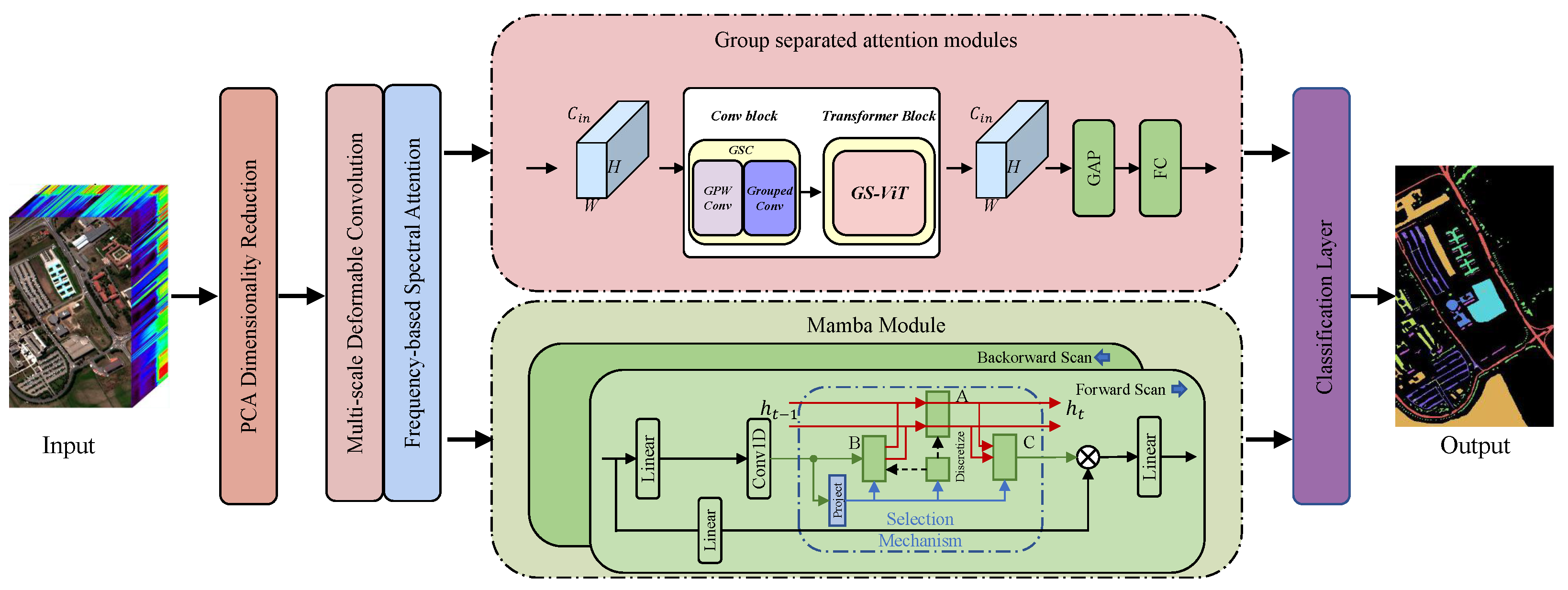
This chapter details the network architecture of FreqMamba, as shown in Figure 1. The pipeline consists of three stages: (1) preprocessing HSI data via multi-scale dynamic convolution combined with frequency-domain transformation; (2) a hybrid architecture of ViT and Mamba for feature learning from spectral and spatial perspectives, respectively; and (3) feature aggregation fed into the classifier for the final result.

3.1. Frequency-Based Multi-Scale Deformable Convolutional Feature Extraction (FMDC)

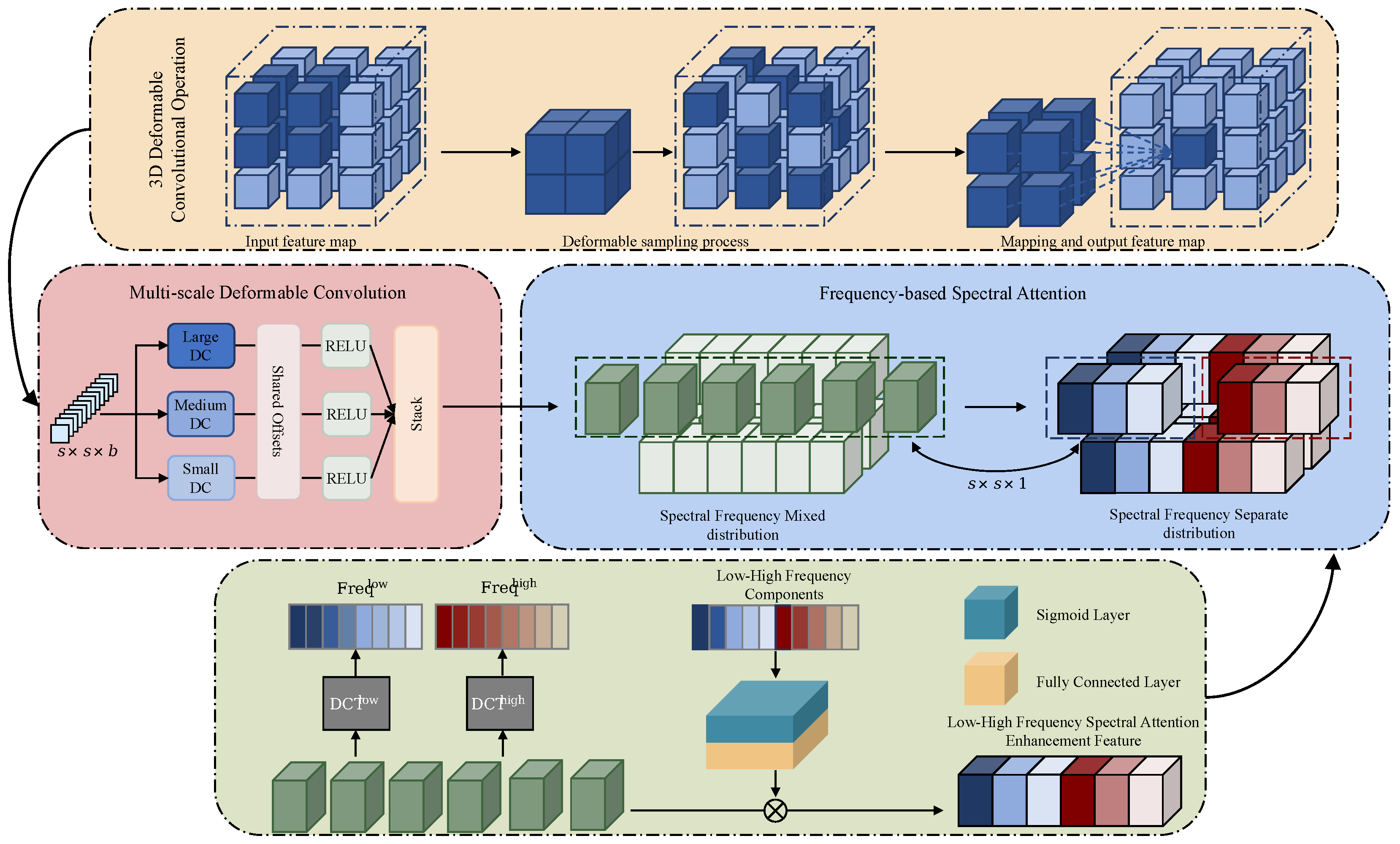
For large-scale HSI data, the sampling positions of standard convolutional kernels are fixed, resulting in a rigid receptive field. When dealing with irregular and complex land surface contours and object shapes, the fixed receptive field struggles to conform precisely to actual ground object boundaries, thereby limiting feature extraction capability. To address this issue, this paper proposes a multi-scale deformable convolutional feature extraction module based on frequency spectrum attention, as shown in Figure 2. Deformable convolution enhances spatial adaptability through learnable sampling offsets, which are predicted based on local feature context. Subsequent frequency-domain attention then refines the convolved features by incorporating global spectral information, thereby supplementing the overall feature representation and indirectly improving the robustness of spatial modeling. The multi-scale deformable convolution processing module will first be introduced below, explaining all computational processes in both the upper and lower branches except for the spectral attention enhancement module; subsequently, the frequency-based spectral attention enhancement module will be described.

3.1.1. Multi-Scale Deformable Convolution Processing

The input to the upper branch is the HSI data D R L × H × W , where l denotes the number of spectral bands. To mitigate the curse of dimensionality, a Principal Component Analysis (PCA) is first applied to D for dimensionality reduction, obtaining D pca R C × H × W . Subsequently, the spatial dimensions are divided into s × s image patches, and a multi-scale deformable convolution (MDC) operation is performed. In this operation, the output of the i-th layer feature at position ( x , y , z ) is calculated as follows:
α i x y z = a , b , c K L ( a , b , c ) · D p c a ( x + a + Δ a , y + b + Δ b , z + c + Δ c ) , β i x y z = a , b , c K M ( a , b , c ) · D p c a ( x + a + Δ a , y + b + Δ b , z + c + Δ c ) , δ i x y z = a , b , c K S ( a , b , c ) · D p c a ( x + a + Δ a , y + b + Δ b , z + c + Δ c ) ,
where K L , K M , and K S represent large-, medium-, and small-scale convolutional kernels, respectively (the specific configuration used in the code is 7 × 7, 5 × 5, and 3 × 3 kernels). To enhance the sampling flexibility, learnable offsets ( Δ a , Δ b , Δ c ) are introduced for each sampling point ( a , b , c ) in the convolutional kernel. To address the issue of non-integer coordinates after offsetting, bilinear interpolation is used to compute the pixel value at D p c a ( x + a + Δ a , y + b + Δ b , z + c + Δ c ) . After performing convolution at the three scales, the resulting feature maps are concatenated and fused via a 1 × 1 × 1 convolution, followed by a residual connection with β i x y z , yielding the fused multi-scale spectral–spatial feature v i x y z :
v i x y z = concat ( α i x y z , β i x y z , δ i x y z ) Filter 1 × 1 × 1 + β i x y z .
In the lower branch, the Extended Multi-Attribute Profile (EMAP) feature D e m a p R C × H × W is first extracted from the original HSI data to enhance spatial detail information using mathematical morphology. Subsequently, D e m a p is divided into s × s patches in the spatial dimensions, and two-dimensional multi-scale deformable convolution is applied to each channel (treated as a 2D image). The feature at position ( x , y ) for the i-th layer is calculated as follows:
α i x y = a , b K L ( a , b ) · D e m a p ( x + a + Δ a , y + b + Δ b ) , β i x y = a , b K S ( a , b ) · D e m a p ( x + a + Δ a , y + b + Δ b ) .
The feature maps from the two scales are concatenated, fused via a 1 × 1 convolution, and then connected residually with β i x y to obtain the output feature at that position:
v i x y = concat ( α i x y , β i x y ) Filter 1 × 1 + β i x y .

3.1.2. Frequency-Based Spectral Attention Enhancement

HSIs inherently represent continuous spectral reflectance profiles. Their frequency-domain transformations—such as the Discrete Cosine Transform (DCT) and Fourier Transform—can reveal global periodic patterns and noise characteristics embedded within the spectral signals. Typically, low-frequency components correspond to macroscopic spectral traits (e.g., overall reflectance levels), while high-frequency components capture fine details (e.g., absorption features and subtle noise edges). Conventional spatial attention mechanisms tend to emphasize spatial context at the expense of high-frequency detail. In contrast, frequency-aware attention enables the simultaneous preservation of low-frequency global information and high-frequency local features, making it particularly effective for distinguishing land-cover categories with visually similar spectral curves but subtle discriminative variations.
Traditional channel attention mechanisms tend to lose high-frequency details when compressing spatial information. Therefore, we introduce a frequency-based spectral attention enhancement module at the end of the upper branch to more effectively enhance key spectral bands.
Traditional attention mechanisms typically use pooling layers to compress channel features, expressed as follows:
a t t = σ ( F C ( ϕ ( X ) ) ) ,
where X is the input feature map, σ is the Sigmoid activation function, FC denotes a fully connected layer, and ϕ is a compression function that reduces a feature map of size C × H × W to a C-dimensional vector. This compression operation can also be expressed using the Discrete Cosine Transform (DCT) as follows:
ϕ h , w = i = 0 H 1 j = 0 W 1 x i , j cos π h H ( i + 1 2 ) cos π w W ( j + 1 2 ) ,
where i 0 , 1 , , H 1 , j 0 , 1 , , W 1 . Building upon this idea, the compression function proposed in this paper retains both low-frequency and high-frequency information of the feature map, and is expressed as follows:
ϕ i , j = c a t i = 0 H 1 j = 0 W 1 x i , j ( sin ( π i ) · sin ( π j ) ) , i = 0 H 1 j = 0 W 1 x i , j .
Based on this idea, the compression function proposed in this paper simultaneously retains low-frequency and high-frequency information of the feature map, and is expressed as follows:
F S _ a t t = σ ( F C ( ϕ i , j ) ) .
Finally, the output features of the upper branch are enhanced by the attention weights, resulting in the enhanced feature map X R C × H × W .

3.2. The Structure of Group-Separated Attention Module

Since different ground objects possess unique spectral reflectance characteristics in specific bands, the numerous spectral channels in HSI also contain key information to distinguish between different ground object markers.

3.2.1. Grouped Convolution

Here, a grouped convolution structure is made up of a grouped pointwise convolution layer with a kernel size of 1 × 1 , a grouped convolution layer with a kernel size of 3 × 3 (set the padding to 1), and a normalization layer. The expression is as follows:
X ˙ i G K = C o n v 3 × 3 C o n v 1 × 1 X i d r , X G R = B a t c h N o r m c o n c a t X ˙ 1 G K , , X ˙ k G K ,
where X i d r R g / k × H × W represents the data after splitting the output of the FMDC module along the channel dimension, and X G K R g × H × W represents the output obtained after concatenating the intermediate results X ˙ i G K R g / k × H × W along the channel dimension and applying normalization processing. The use of a grouped design offers the following two advantages: (1) It reduces the number of convolution parameters to 1 / k of the original, making the network more suitable for deployment on parallel computing devices. (2) Convolutions within each group focus on extracting local features from specific spectral intervals, which can preliminarily remove redundant information and enhance key information in the spectrum, thereby improving the efficiency and accuracy of subsequent attention mechanisms in establishing global spectral responses.

3.2.2. Group-Separable Self-Attention Structure

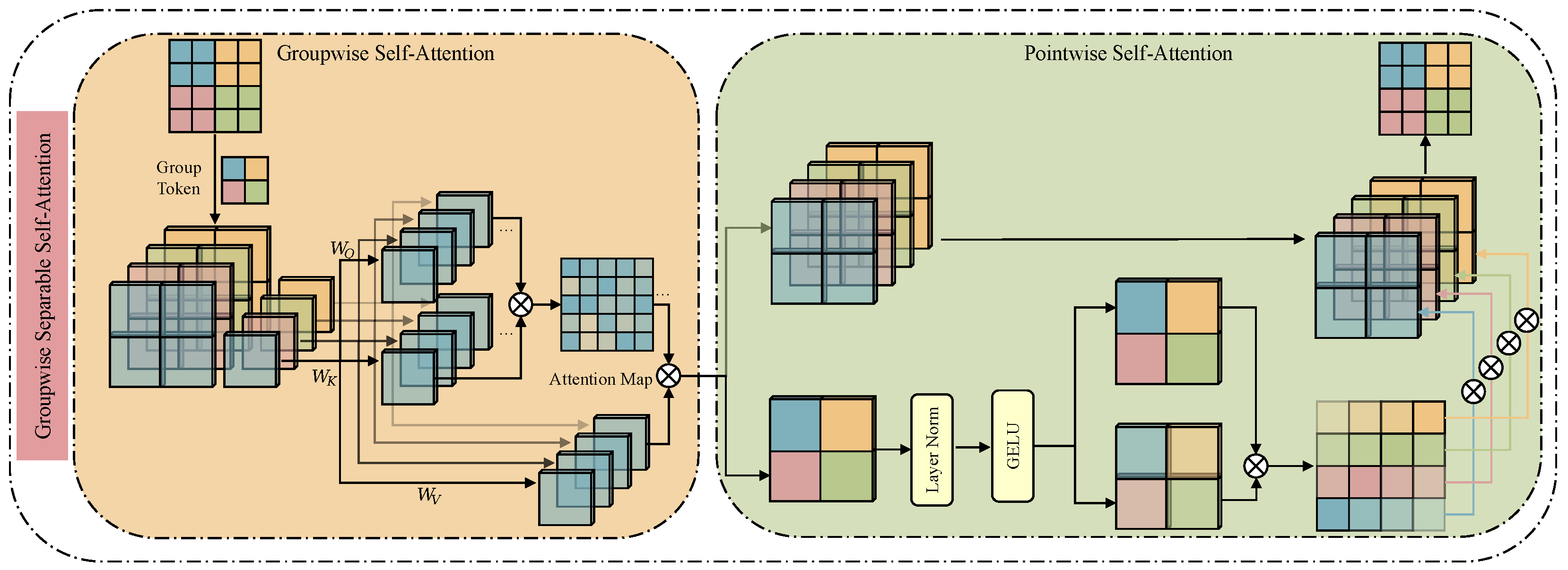
Traditional ViT has high computational complexity and lacks fine-grained local perception capabilities. Here, we use group-separated self-attention. The grouping mechanism enables efficient modeling of both local and global spectral characteristics. At the local level, convolutional groups focus on specific spectral intervals to extract features independently, effectively reducing cross-band interference and enhancing the representation of local spectral structures. Globally, a group token is introduced to aggregate and exchange information across groups. This token summarizes features from each group and participates in global attention computation, thereby modeling long-range dependencies across spectral intervals. This design preserves fine-grained spectral details while significantly improving feature discriminability through global interaction.
As shown in Figure 3, the spatial dimension of the input feature map is first divided into several non-overlapping subgraphs of the same size, each corresponding to a group. Then, for each group, a “group token” is automatically generated. This token is a single pixel that serves as the core feature representation of the corresponding group. Next, the spatial pixels of each group are flattened into a 1-dimensional form to facilitate their concatenation with the “group token” for subsequent operations. Specifically: for the input data X G K R g × H × W , its shape is reshaped from g × ( m · h ) × ( m · w ) to m 2 × g × ( h · w ) , where m 2 represents the number of groups, and ( h · w ) represents the number of elements in each group. The “group token” is generated by random initialization on [ 0 , 1 ] , with a shape of m 2 × g × 1 . The two are concatenated to obtain new data X a t t n with a shape of m 2 × g × ( h · w + 1 ) .
In the self-attention mechanism, the method for generating Q, K, and V from the 1D pixel data is as follows: use a traditional 1D convolution to expand the number of the input channel of the data to three times the original, then split the expanded result into three groups, corresponding to Q, K, and V, respectively:
Q , K , V = S p l i t ( C o n v 1 ( X a t t n ) ) ,
where C o n v 1 is a 1D convolution with a window size of 1, and the output channel number is three times the input channel number. S p l i t means evenly dividing along the channel dimension into three groups, obtaining Q , K , V R m 2 × g × ( h · w + 1 ) . The global response of the spectral channels within each group is calculated as follows: K and V, respectively:
X ˙ a t t n = S o f t M a x Q K T d k V ,
where d k represents the dimension of the matrix K, and X ˙ a t t n R m 2 × g × ( h · w + 1 ) .
The channel attention X ˙ a t t n obtained above is essentially the global response of the spectral channels within each group, which means that the groups are independent of each other. How to correlate the independent groups? At this point, the previously set “group token” plays a key role: generate “Q” and “K” from the “group token” to obtain the attention relationship between groups and use the features of each group as “V” for global feature fusion. Specifically, first separate the “group token” from X ˙ a t t n , denoted as X g t R m 2 × g × 1 , then perform normalization and convolution operations to obtain
Q g t , K g t = S p l i t C o n v X g t ,
where Q g t , K g t R m 2 × g × h · w . Then, the global response is calculated based on the inter-group attention relationships:
X ¨ a t t n = S o f t M a x Q g t ( K g t ) T d k V ^ ,
where X ¨ a t t n R m 2 × g × ( h · w ) , and V ^ represents the remaining part of X ˙ a t t n after removing the “group token”.
Finally, reshape X ¨ a t t n to g × H × W and add it to the output of the grouped convolution layer to obtain the final output of the module, which means
X s p a = X G K + X ¨ a t t n .

3.3. Mamba

The Mamba branch aims to effectively classify HSI by leveraging Mamba’s ability to capture dependencies in both the spectral and spatial dimensions. The core of this module is the use of SSM, which serves as a fundamental mathematical modeling framework. This model maps input signals to a latent state space through a set of ordinary differential equations (ODEs), subsequently reconstructing the output sequence, thereby systematically characterizing the dynamic properties and temporal dependencies within the system. The continuous form of SSM can be expressed as follows:
h ( t ) = A h ( t ) + B x ( t ) , y ( t ) = C h ( t ) .
Since the input data is discrete, the continuous SSM must be “discretized” to handle discrete sequences. Mamba uses the Zero-Order Hold (ZOH) method for discretization. That is, given an input step size Δ (can be understood as a time interval), the continuous parameters ( A , B ) are converted into discrete parameters ( A ¯ , B ¯ ) through the following equations:
A ¯ = exp ( Δ A ) , B ¯ = Δ A 1 ( exp ( Δ A ) I ) · Δ B .
This discretization captures the system dynamics precisely at each time step, allowing states to be updated at discrete intervals. The discretized SSM can be expressed as follows:
h t = A ¯ h t 1 + B ¯ x t , y t = C h t .
Based on this, we propose a novel two-branch Mamba with bidirectional scanning. The output X R C × H × W of the FMDC module is first flattened into a complete forward scan sequence S R C × H · W by spatial dimension, and, subsequently, the spatial feature output X s p e is obtained through the standard mamba block:
X s p e = M a m b a ( S ) + M a m b a ( F l i p ( S ) ) ,
where F l i p represents the reversal of the data sequence.
Finally, the two-branch results are fed into the linear classifier to generate the final prediction. This process is formulated as follows:
y ^ = F C G A P X s p a + X s p e
where G A P denotes the global average pooling operation, F C is a fully connected layer, and y ^ represents the predicted class logits.

4. Results

4.1. Datasets and Setting

4.1.1. Datasets

A total of five published benchmark datasets are used in our experiments, including the QUH-Tangdaowan, QUH-Qingyun, QUH-Pingan [45], Houston2013, and Pavia University (PU).
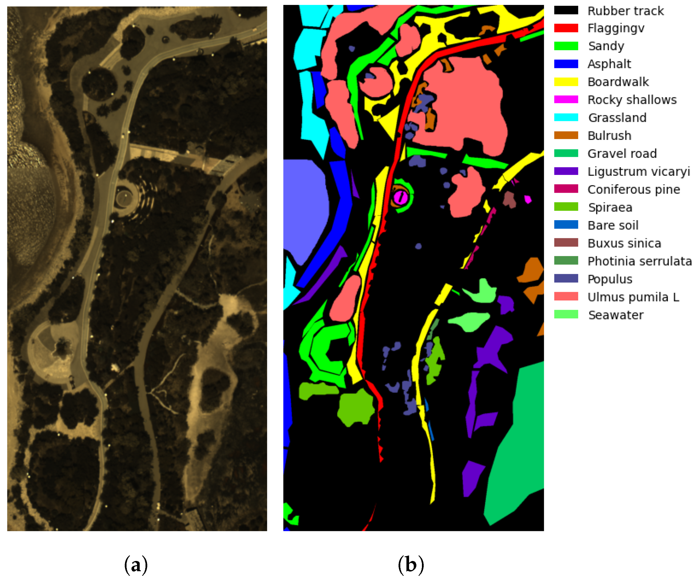
  • QUH-Tangdaowan: The dataset was collected by running a UAV at an altitude of 300 m with a spatial resolution of about 0.15 m, including a total of 176 bands with wavelengths ranging from 400 to 1000 nm and an image pixel size of 1740 × 860. Table 1 and Figure 4 illustrate the number of training, validation, test data in this dataset, and real ground feature coverage map.
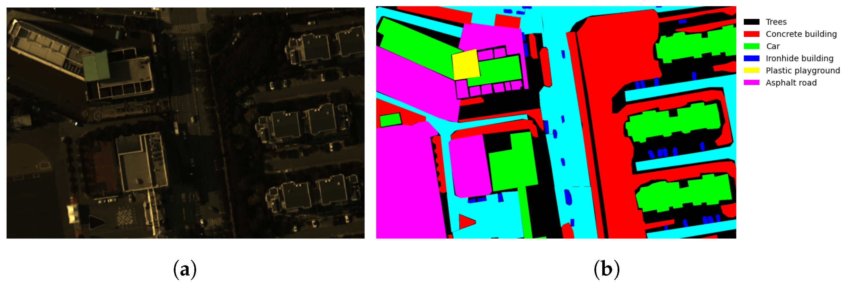
  • QUH-Qingyun: This dataset was collected by a drone operating at an altitude of 300 m. The captured image has a pixel size of 880 × 1360, 176 bands, ranging from 400 to 1000 nm, and a spatial resolution of approximately 0.15 m. Table 2 and Figure 5 illustrate the quantity of training, validation, test data in this dataset, and real ground feature coverage map.
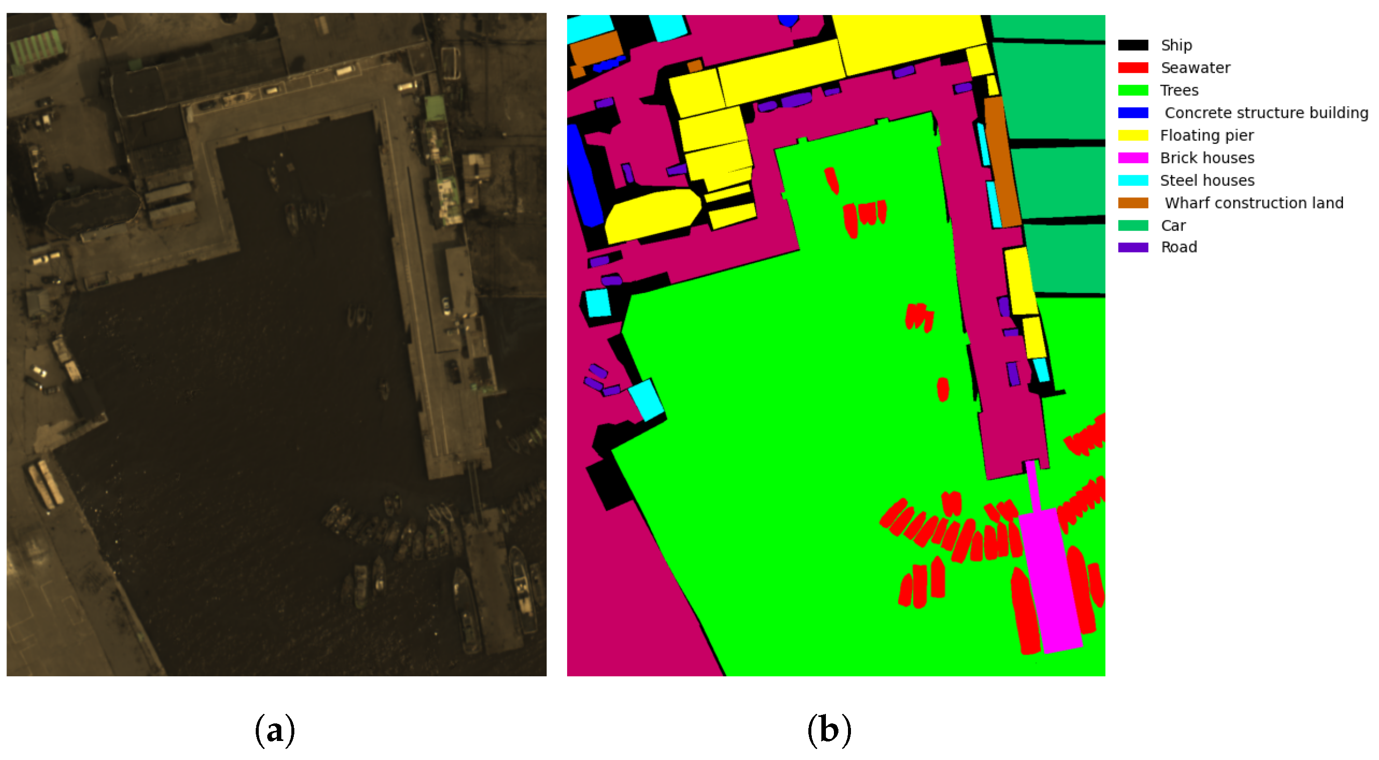
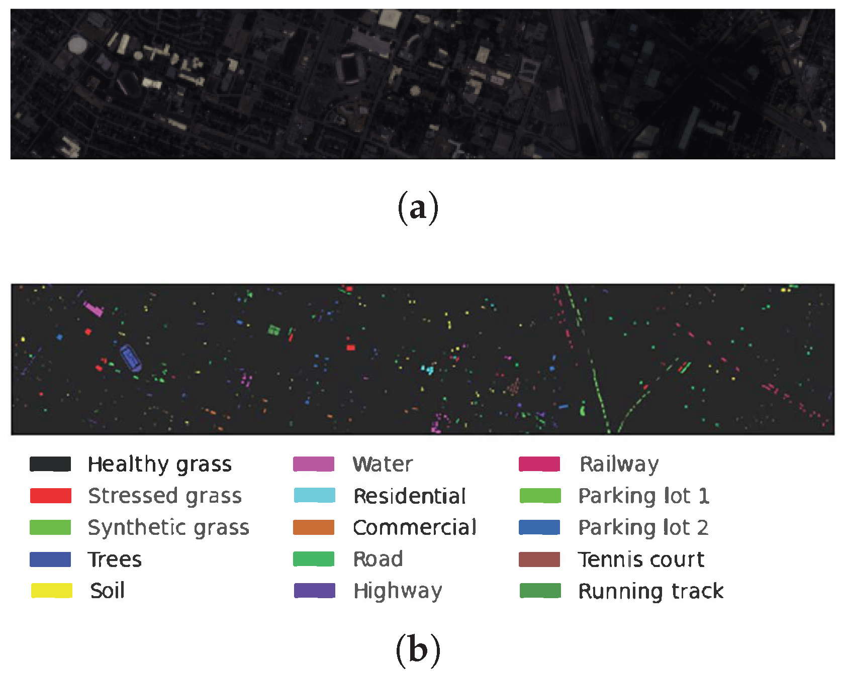
  • QUH-Pingan: The UAV operates the acquisition at an altitude of 200 m above the ground with a spatial resolution of approximately 0.10 m. The dataset includes 176 bands with wavelengths ranging from 400 to 1000 nm, and the image pixel size is 1230 × 1000. Table 3 and Figure 6 show the number of training, validation, test data in this HSI dataset, and real ground feature coverage map.
  • Houston2013: This scene was captured by the ITRES CASI-1500 sensor over the campus of the University of Houston and its adjacent rural areas, and was used in the 2013 GRSS Data Fusion Competition. This data includes 144 spectral bands and 349 × 1905 pixels in the 380–1050 nm region, with a spatial resolution of 2.5 m. Table 4 and Figure 7 show the number of training, validation, test data in this HSI dataset, and real ground feature coverage map.
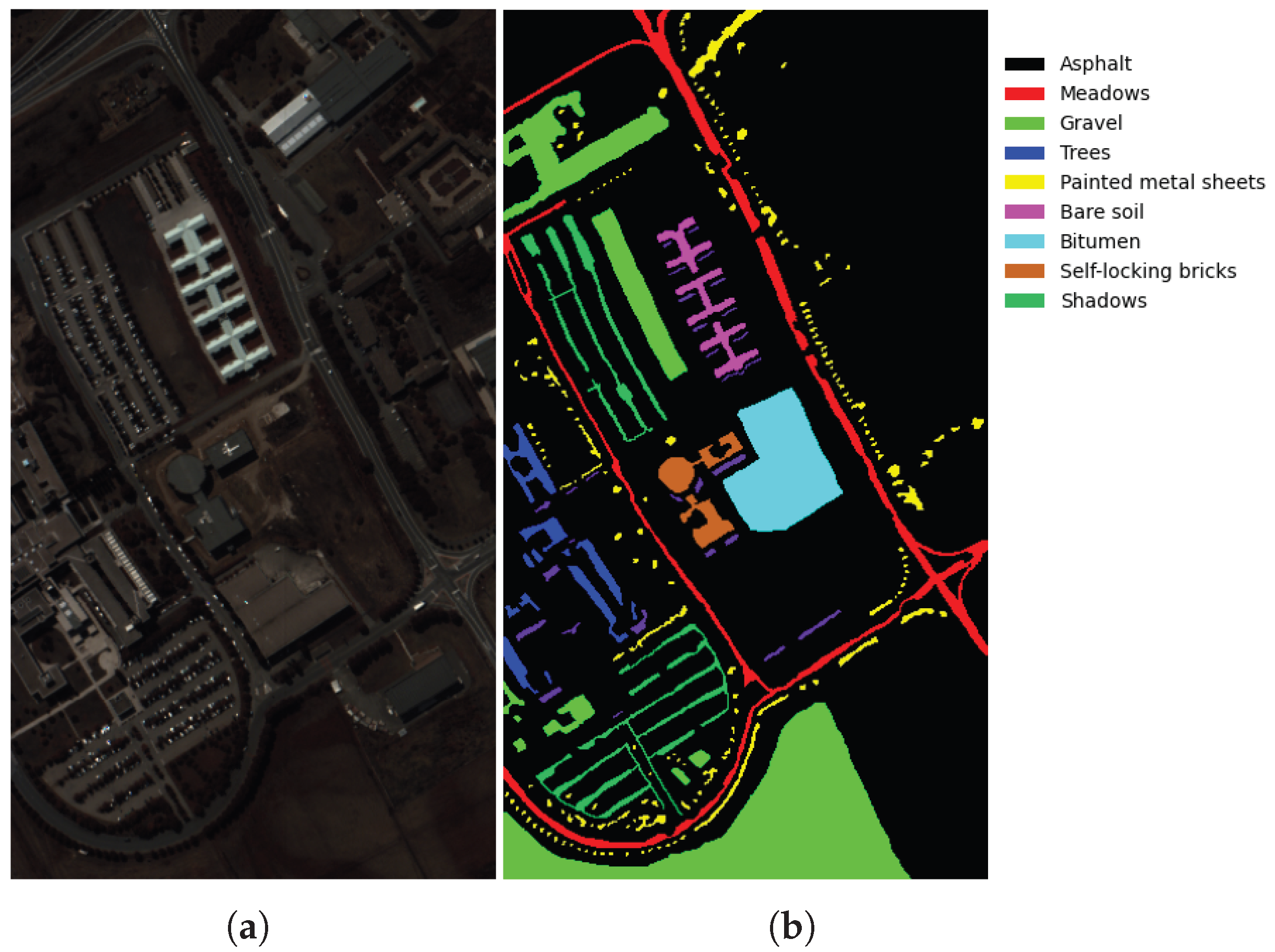
  • PU: The images of the University of Pavia were captured by the Reflection Optical Systems Imaging Spectroscope-3 (ROSIS-3) sensor at the University of Pavia and its surroundings in Pavia, Italy. This image consists of 610 × 340 pixels, with a spatial resolution of 1.3 m per pixel and 115 bands. After removing 12 noise bands, experiments were conducted on the remaining 103 bands. Table 5 and Figure 8 show the number of training, validation, test data in this HSI dataset, and real ground feature coverage map.

4.1.2. Evaluation Metrics

To quantify the performance of classification methods, three standard measures were used: overall accuracy (OA), average accuracy (AA), and Kappa coefficient ( κ ). These metrics are calculated based on the confusion matrix, which provides a detailed breakdown of the classification results by comparing the predicted labels against the ground truth.
OA is the most intuitive metric, representing the proportion of correctly classified pixels out of the total number of test pixels. It offers a general assessment of the classifier’s performance. The formula for OA is defined as follows:
O A = i = 1 k T P i N
where k denotes the total number of land-cover classes, T P i (True Positives for class i) is the number of pixels correctly classified into class i, and N is the total number of pixels in the test set.
AA is the mean of the Producer’s Accuracy for all individual classes. This metric is particularly important for evaluating performance on imbalanced datasets, as it assigns equal weight to each class, preventing the overall performance from being dominated by classes with a large number of samples. It is calculated as follows:
A A = 1 k i = 1 k T P i C i
where C i is the total number of pixels that truly belong to class i in the ground truth (the sum of T P i and F N i , where F N i are the false negatives for class i).
κ measures the agreement between the classification map and the ground truth data while accounting for the agreement that might occur by chance. A value of 1 indicates perfect agreement, while a value of 0 indicates agreement no better than random chance. It provides a more robust evaluation than OA by considering random correctness. The Kappa coefficient is calculated as follows:
κ = O A p e 1 p e
where p e represents the hypothetical probability of chance agreement, which is computed from the confusion matrix. Specifically, p e is the sum of the products of the row and column totals for each class, divided by the square of the total number of samples:
p e = i = 1 k P i · × P · i N 2
where P i · is the total number of pixels predicted as class i (row sum), and P · i is the total number of pixels truly belonging to class i (column sum).
These three metrics complement each other: OA provides a global performance overview, AA ensures balanced evaluation across all classes, and κ validates the statistical significance of the classification results. In the subsequent sections, these metrics will be used to conduct a thorough comparative analysis of the proposed FreqMamba framework against other state-of-the-art methods.

4.1.3. Comparison Methods

We conducted comprehensive comparisons with state-of-the-art methods across different architectural paradigms: CNN-based (e.g., HybridSN [15], A2S2K [46], and GMA_NET [47]), Transformer-based (e.g., SpectralFormer [21], GSC-ViT [48], MHCFormer [49]), and SSM-based (e.g., 3DSS-Mamba [31], MambaHSI [50], and HSI-MFormer [51]).

4.1.4. Setting

During the entire experimental process, the training set was randomly selected for each experiment and repeated five times to obtain the average result and standard deviation of each index and reduce the influence of random operations. All experiments were conducted on a server equipped with an Intel(R) Xeon(R) Gold 6326 CPU, an NVIDIA RTX 4090 GPU, and 120 GB RAM. The comparative model codes run in the experiments are all publicly available. All models were trained with consistent proportions on different datasets, and Adam optimizer was used to optimize the network parameters with batch size 128 and epochs set to a fixed value of 120. The other hyperparameters, such as patch size and learn rate, are set to the optimal parameters in their respective original papers. For our proposed model, the learn rate is set to 0.001, the patch size is set to 12 × 12, and the number of bands after PCA dimensionality reduction is 30.

4.2. Result Analysis

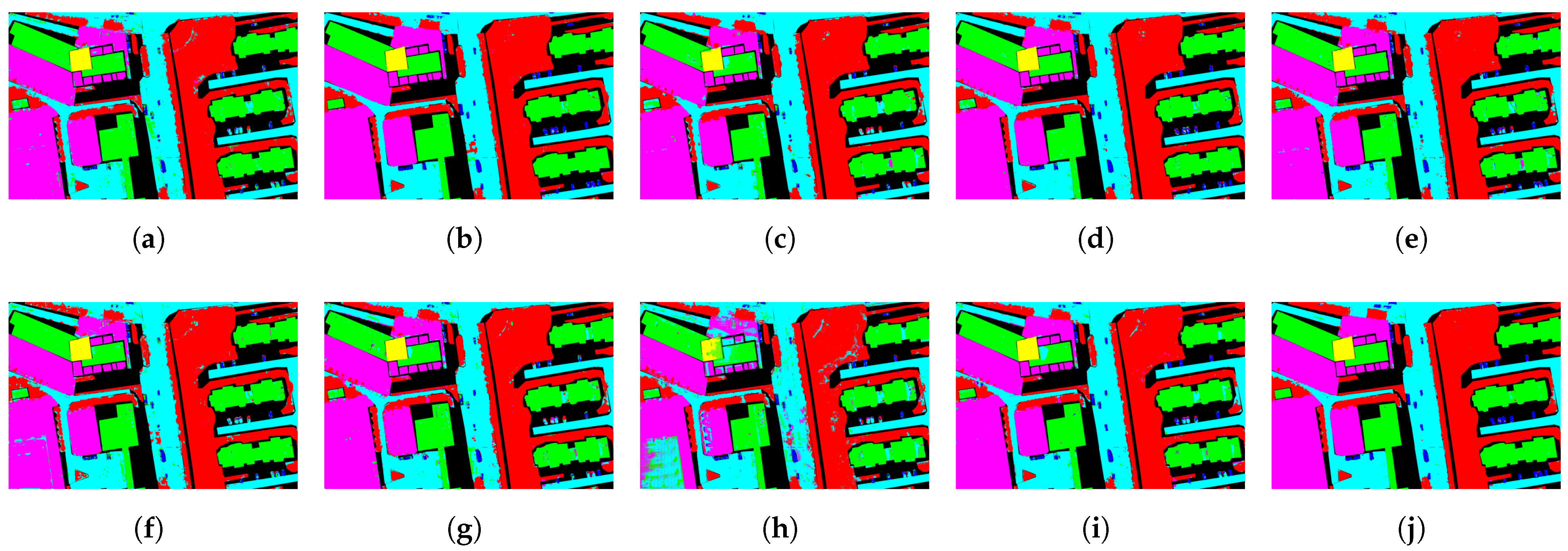
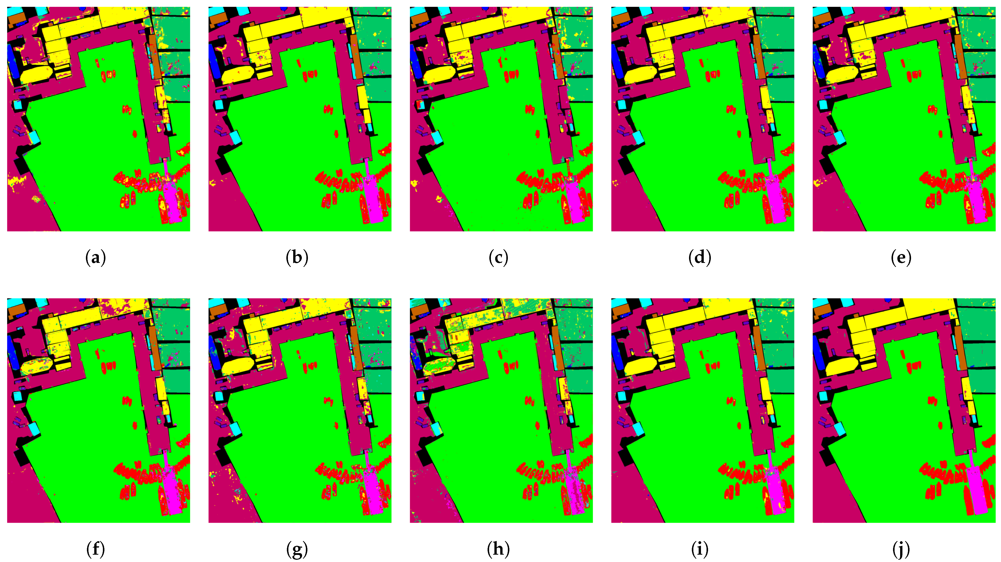
In this section, we present a comprehensive analysis of the experimental results obtained from the QUH-Tangdaowan, QUH-Qingyun, QUH-Pingan, Houston2013, and PU datasets, as shown in Table 6, Table 7, Table 8, Table 9 and Table 10 and Figure 9, Figure 10, Figure 11, Figure 12 and Figure 13. Our analysis focuses on evaluating the overall performance of the proposed FreqMamba in terms of state-of-the-art comparison methods for CNN-based, Transformer-based, and SSSM-based categories, as well as examining the accuracy and model robustness for each category.
The proposed model achieves the highest OA, AA, and κ on all five datasets. On the QUH-Tangdaowan dataset (Table 6), FreqMamba achieved a 96.48% OA, a 93.41% AA, and a 95.98% κ , outperforming all comparison methods in overall and average accuracy. Similarly, for the QUH-Pingan dataset (Table 7), the OA of FreqMamba is 95.58%, AA is 91.71%, and κ is 94.14%. On the QUH-Qingyun dataset (Table 8), the learning ability and robustness of FreqMamba were verified once again, achieving the highest scores of 97.47%, 93.52%, and 96.22%, respectively on the three metrics of OA, AA, and κ . It also achieved optimal performance on the Houston2013 and PU datasets. The results strongly verified the effectiveness of the proposed framework.
The results of the comparison between FreqMamba and the representative methods of three architectures clearly reveal the significant advantages of our proposed hybrid architecture. Experiments on the QHU-Tangdaowan dataset show that while CNN-based methods perform moderately well on some categories, their OA is generally lower than state-of-the-art methods based on Transformer and SSM, highlighting their inherent limitations in modeling long-distance spectral–spatial dependencies. Transformer-based methods effectively capture the global context through the self-attention mechanism and achieve competitive classification accuracy, becoming the current strong baseline model. However, our model still robustly outperforms these Transformer models in overall performance, which confirms that the strategy of combining the advantages of convolutions in local feature extraction with the ability of SSM in efficient global sequence modeling is more effective for HSIC.
In addition, by performing an in-depth analysis of the classification accuracy for each land cover class, we evaluate FreqMamba’s performance on challenging classes where training samples are scarce. As shown in Table 6, for classes with very few labeled samples, such as “Spiraea” (C12), “Bare soil” (C13), and “Buxus sinica” (C14), most of the comparison methods showed a significant decline in classification accuracy and a sharp increase in standard deviation. For example, the accuracy of GMA_Net on C12 and C14 is as low as about 64% and 79% respectively, and the standard variation increases to 13.16 and 5.13 respectively. In contrast, FreqMamba shows significantly better and more stable performance on these categories, which indicates that our model is more robust in dealing with the class imbalance problem and can effectively learn discriminative features even from sparse samples. This robustness is further reflected in the generally lower standard deviation of FreqMamba in OA, AA, and κ . Compared with a variety of comparison methods, its performance has less volatility and higher stability, which verifies the effectiveness and reliability of the proposed method.

4.3. Complexity Analysis

As summarized in Table 11, FreqMamba demonstrates a pronounced advantage in computational efficiency. Among CNN-based models, HybridSN and A2S2K exhibit relatively high parameter counts (3.991 M and 0.333 M, respectively) and computational complexity (431.068 M and 225.454 M FLOPs, respectively), with FLOPs substantially exceeding those of other modern architectures. Within Transformer-based models, SpectralFormer and GSC-ViT maintain better-controlled parameter numbers (approximately 0.31 M and 0.17 M), while GSC-ViT also achieves relatively low computational cost (6.16 M FLOPs). In contrast, MHCFormer shows significantly higher parameter count (3.391 M) and FLOPs (274.974 M).
Mamba-based models generally achieve high computational efficiency, with 3DSS-Mamba and MambaHSI in particular operating at low parameter counts (0.12–0.13 M) and FLOPs (2.2–6.8 M). FreqMamba requires 0.256–0.308 M parameters, which is comparable to other efficient Mamba and Transformer models, while its FLOPs (8.2–8.3 M) are markedly lower than most CNN and Transformer baselines and only slightly higher than those of 3DSS-Mamba.
Furthermore, FreqMamba maintains consistent parameter counts and computational costs across the three datasets, whereas HSI-MFormer exhibits large fluctuations in FLOPs—reaching 148.542 M on Tangdaowan but dropping to 74.271 M on other datasets. These results indicate that FreqMamba effectively incorporates the low-complexity characteristics of efficient architectures, demonstrates strong generalization capability and stability, and strikes an desirable balance between computational efficiency and model performance.

5. Discussion

To further validate the effectiveness of our proposed method, we carried out an extensive discussion based on the experimental results. This includes a systematic ablation study on the QUH-Tangdaowan dataset, to quantitatively evaluate the key contributions of FMDC, Group-Separated Attention, and Mamba module in the overall framework.

5.1. Impact of FMDC

The ablation study results presented in Table 12 clearly demonstrate the pivotal role of the Frequency-based Multi-scale Deformable Convolutional (FMDC) module in our proposed framework. The complete model achieved optimal performance (OA: 96.17%, AA: 95.55%, κ : 95.65), while any simplification or removal of this module led to substantial degradation across all evaluation metrics. Specifically, replacing the FMDC module with standard 3D convolution resulted in noticeable declines in all three metrics (OA decreased by 3.25%), underscoring the advantage of the multi-scale and deformable design in enhancing feature extraction capability. Furthermore, removing only the frequency-domain processing component caused an even more pronounced performance drop (OA decreased by 7.93%), indicating that frequency-domain information is essential for capturing discriminative features in HSI data. When the entire FMDC module was excluded, FreqMamba’s performance deteriorated dramatically (OA decreased by 14.25%, and the kappa coefficient dropped by 15.40%), providing compelling evidence that the FMDC module constitutes the primary contributor to FreqMamba’s core performance. By effectively integrating spatial–frequency multi-scale information, the FMDC module significantly enhances FreqMamba’s representational capacity and classification accuracy.

5.2. Impact of ViT

The ablation experimental results in Table 13 reveal the critical impact of group size (Group_Size) in the ViT branch on model performance, which manifests as a typical inverted “U” shaped relationship: when the group size is set to 3 or 4 (4 is chosen in the structure), FreqMamba achieves the best performance on the QUH-Tangdaowan dataset (OA of 96.17% and 96.48%, respectively), indicating that a moderate grouping range can most effectively balance local feature extraction with global context modeling capabilities. However, when the group size is too small, FreqMamba’s performance declines (OA: 94.81%) due to limited receptive fields that struggle to establish long-range dependencies, and when the group size is too large (=6 or 12), the larger groups include too many unrelated pixels, diluting the significance of key local features and causing a sharp deterioration in performance (OA drops to 94.55% and 93.56%). This result clearly verifies the effectiveness of the grouped attention mechanism and identifies the optimal group size parameters.

5.3. Impact of Mamba

The ablation results in Table 14 demonstrate the significant contribution of the Mamba branch to the overall model performance. While the removal of the Mamba branch leads to a moderate decrease in overall accuracy (OA) by 1.70% and Kappa coefficient by 1.97%, it causes a substantial drop of 9.58% in average accuracy (AA). This pronounced decline in AA indicates that the Mamba branch plays a critical role in maintaining classification performance across different land-cover categories, particularly for those classes that are more challenging to classify. The results suggest that the Mamba branch effectively enhances FreqMamba’s capability to capture sequential dependencies in the data, thereby ensuring more balanced and robust classification results across all categories.

5.4. Impact of Frequency-Aware Methods

To evaluate the importance of frequency-domain information in HSIC, we also conducted experiments comparing the performance of the proposed FMDC module against several frequency-aware methods, including average pooling, Discrete Cosine Transform (DCT), Fourier Transform, and Gabor Filter. The experimental results are shown in Table 15. The complete FMDC model achieved the best performance across all metrics—overall accuracy (OA: 96.17%), average accuracy (AA: 95.55%), and Kappa coefficient ( κ : 95.65%)—significantly outperforming other approaches. Average pooling yielded the lowest results (a 6.13% drop in OA), due to the loss of high-frequency details caused by its simplistic compression. The conventional DCT method (4.83% OA reduction) showed limited capability in extracting high-frequency information. While Fourier Transform (2.91% OA decrease) effectively captured global spectral patterns, it lacked dynamic adaptability. Gabor filtering (4.63% OA drop) suppressed noise but also weakened critical high-frequency features.
In contrast, FMDC integrates multi-scale deformable convolution with frequency-domain attention to dynamically focus on discriminative frequency bands, effectively balancing low-frequency spectral trends and high-frequency local details. This leads to improved robustness to complex land-cover boundaries and enhanced classification accuracy. The experiments confirm the distinct advantage of FMDC in utilizing frequency-domain information.

6. Conclusions

The proposed FreqMamba framework introduces a Mamba module with linear complexity combined with deformable convolution, enabling effective joint modeling of long-range spectral dependencies and adaptive spatial features in HSI. This approach dynamically focuses on discriminative frequency bands and spatial details. While significantly improving computational efficiency, it successfully overcomes the limitations of traditional CNN-Transformer hybrid models, demonstrating substantial advantages in both classification accuracy and robustness.
Experimental results on the QUH-Tangdaowan, QUH-Qingyun, QUH-Pingan, Houston2013, and PU benchmark datasets demonstrated FreqMamba’s superior performance. Our approach achieved the highest overall accuracy (OA), average accuracy (AA), and Kappa coefficient, outperforming state-of-the-art CNN, Transformer, and SSM-based methods. This confirms the robustness, high generalization capability, and effectiveness of the framework in handling hyperspectral data with high interclass similarity and significant intra-class variability.
Although FreqMamba has theoretical advantages in terms of computational efficiency, the frequency-domain transformation and dynamic convolution operations in its multi-branch architecture put forward high requirements for hardware parallelization support, and special operator optimization is still needed. At the same time, the frequency-domain attention mechanism is sensitive to spectral perturbations caused by illumination changes, which may lead to feature distortion in extreme shadows or strong reflection conditions.
For future work, we will focus on developing adaptive group size mechanisms to reduce hyperparameter sensitivity, exploring lightweight designs for edge-device deployment, and extending the framework to tasks such as hyperspectral segmentation and change detection. These efforts aim to enhance practicality while maintaining FreqMamba’s efficiency and interpretability.
Author Contributions

Conceptualization, T.Z. and J.Z.; methodology, T.Z. and Z.Z.; software, J.Z. and Z.Z.; validation, T.Z., J.Z. and Z.Z.; writing—original draft preparation, T.Z. and J.Z.; writing—review and editing, T.Z. and Z.Z. All authors have read and agreed to the published version of the manuscript.

Funding

This research was funded by Shandong Provincial Natural Science Foundation Grant ZR2023LZH014.

Data Availability Statement

Datas openly available in public repositories.

Conflicts of Interest

The authors declare no conflicts of interest.

References

  1. Bioucas-Dias, J.M.; Plaza, A.; Camps-Valls, G.; Scheunders, P.; Nasrabadi, N.; Chanussot, J. Hyperspectral Remote Sensing Data Analysis and Future Challenges. IEEE Geosci. Remote Sens. Mag. 2013, 1, 6–36. [Google Scholar] [CrossRef]
  2. He, L.; Li, J.; Liu, C.; Li, S. Recent Advances on Spectral–Spatial Hyperspectral Image Classification: An Overview and New Guidelines. IEEE Trans. Geosci. Remote Sens. 2018, 56, 1579–1597. [Google Scholar] [CrossRef]
  3. Pallocci, M.; Treglia, M.; Passalacqua, P.; Luca, L.D.; Zanovello, C.; Mazzuca, D.; Guarna, F.; Gratteri, S.; Marsella, L.T. Forensic applications of hyperspectral imaging technique: A narrative review. Med.-Leg. J. 2022, 90, 216–220. [Google Scholar] [CrossRef]
  4. Zhao, G.; Ye, Q.; Sun, L.; Wu, Z.; Pan, C.; Jeon, B. Joint Classification of Hyperspectral and LiDAR Data Using a Hierarchical CNN and Transformer. IEEE Trans. Geosci. Remote Sens. 2023, 61, 5500716. [Google Scholar] [CrossRef]
  5. Wu, L.; Fang, L.; Yue, J.; Zhang, B.; Ghamisi, P.; He, M. Deep Bilateral Filtering Network for Point-Supervised Semantic Segmentation in Remote Sensing Images. IEEE Trans. Image Process. 2022, 31, 7419–7434. [Google Scholar] [CrossRef]
  6. Lv, M.; Li, W.; Chen, T.; Zhou, J.; Tao, R. Discriminant Tensor-Based Manifold Embedding for Medical Hyperspectral Imagery. IEEE J. Biomed. Health Inform. 2021, 25, 3517–3528. [Google Scholar] [CrossRef]
  7. Camps-Valls, G.; Gomez-Chova, L.; Munoz-Mari, J.; Vila-Frances, J.; Calpe-Maravilla, J. Composite kernels for hyperspectral image classification. IEEE Geosci. Remote Sens. Lett. 2006, 3, 93–97. [Google Scholar] [CrossRef]
  8. Melgani, F.; Bruzzone, L. Classification of hyperspectral remote sensing images with support vector machines. IEEE Trans. Geosci. Remote Sens. 2004, 42, 1778–1790. [Google Scholar] [CrossRef]
  9. Huang, W.; Huang, Y.; Wang, H.; Liu, Y.; Shim, H.J. Local Binary Patterns and Superpixel-Based Multiple Kernels for Hyperspectral Image Classification. IEEE J. Sel. Top. Appl. Earth Obs. Remote Sens. 2020, 13, 4550–4563. [Google Scholar] [CrossRef]
  10. Su, H.; Yu, Y.; Wu, Z.; Du, Q. Random Subspace-Based k-Nearest Class Collaborative Representation for Hyperspectral Image Classification. IEEE Trans. Geosci. Remote Sens. 2021, 59, 6840–6853. [Google Scholar] [CrossRef]
  11. Tong, F.; Zhang, Y. Spectral–Spatial and Cascaded Multilayer Random Forests for Tree Species Classification in Airborne Hyperspectral Images. IEEE Trans. Geosci. Remote Sens. 2022, 60, 4411711. [Google Scholar] [CrossRef]
  12. Wei, H.; Yangyu, H.; Li, W.; Fan, Z.; Hengchao, L. Deep Convolutional Neural Networks for Hyperspectral Image Classification. J. Sens. 2015, 2015, 258619. [Google Scholar]
  13. Zhao, W.; Du, S. Spectral–Spatial Feature Extraction for Hyperspectral Image Classification: A Dimension Reduction and Deep Learning Approach. IEEE Trans. Geosci. Remote Sens. 2016, 54, 4544–4554. [Google Scholar] [CrossRef]
  14. Ben Hamida, A.; Benoit, A.; Lambert, P.; Ben Amar, C. 3-D Deep Learning Approach for Remote Sensing Image Classification. IEEE Trans. Geosci. Remote Sens. 2018, 56, 4420–4434. [Google Scholar] [CrossRef]
  15. Roy, S.K.; Krishna, G.; Dubey, S.R.; Chaudhuri, B.B. HybridSN: Exploring 3-D–2-D CNN Feature Hierarchy for Hyperspectral Image Classification. IEEE Geosci. Remote Sens. Lett. 2020, 17, 277–281. [Google Scholar] [CrossRef]
  16. He, M.; Li, B.; Chen, H. Multi-scale 3D deep convolutional neural network for hyperspectral image classification. In Proceedings of the 2017 IEEE International Conference on Image Processing (ICIP), Beijing, China, 17–20 September 2017; pp. 3904–3908. [Google Scholar]
  17. Sun, L.; Wang, X.; Zheng, Y.; Wu, Z.; Fu, L. Multiscale 3-D–2-D Mixed CNN and Lightweight Attention-Free Transformer for Hyperspectral and LiDAR Classification. IEEE Trans. Geosci. Remote Sens. 2024, 62, 2100116. [Google Scholar] [CrossRef]
  18. Yang, J.; Wu, C.; Du, B.; Zhang, L. Enhanced Multiscale Feature Fusion Network for HSI Classification. IEEE Trans. Geosci. Remote Sens. 2021, 59, 10328–10347. [Google Scholar] [CrossRef]
  19. Vaswani, A.; Shazeer, N.; Parmar, N.; Uszkoreit, J.; Jones, L.; Gomez, A.N.; Kaiser, L.; Polosukhin, I. Attention is all you need. In Proceedings of the NIPS’17: 31st International Conference on Neural Information Processing Systems, Red Hook, NY, USA, 4–9 December 2017; pp. 6000–6010. [Google Scholar]
  20. Heo, B.; Yun, S.; Han, D.; Chun, S.; Choe, J.; Oh, S.J. Rethinking Spatial Dimensions of Vision Transformers. In Proceedings of the IEEE/CVF International Conference on Computer Vision, Montreal, QC, Canada, 10–17 October 2021; pp. 11936–11945. [Google Scholar]
  21. Hong, D.; Han, Z.; Yao, J.; Gao, L.; Zhang, B.; Plaza, A.; Chanussot, J. SpectralFormer: Rethinking Hyperspectral Image Classification With Transformers. IEEE Trans. Geosci. Remote Sens. 2022, 60, 5518615. [Google Scholar] [CrossRef]
  22. He, X.; Chen, Y.; Li, Q. Two-Branch Pure Transformer for Hyperspectral Image Classification. IEEE Geosci. Remote Sens. Lett. 2022, 19, 6015005. [Google Scholar] [CrossRef]
  23. Wu, K.; Fan, J.; Ye, P.; Zhu, M. Hyperspectral Image Classification Using Spectral–Spatial Token Enhanced Transformer With Hash-Based Positional Embedding. IEEE Trans. Geosci. Remote Sens. 2023, 61, 5507016. [Google Scholar] [CrossRef]
  24. Zhao, F.; Li, S.; Zhang, J.; Liu, H. Convolution Transformer Fusion Splicing Network for Hyperspectral Image Classification. IEEE Geosci. Remote Sens. Lett. 2023, 20, 5501005. [Google Scholar] [CrossRef]
  25. Yang, H.; Yu, H.; Zheng, K.; Hu, J.; Tao, T.; Zhang, Q. Hyperspectral Image Classification Based on Interactive Transformer and CNN with Multilevel Feature Fusion Network. IEEE Geosci. Remote Sens. Lett. 2023, 20, 5507905. [Google Scholar] [CrossRef]
  26. Qin, Z.; Zhang, P.; Wu, F.; Li, X. FcaNet: Frequency Channel Attention Networks. In Proceedings of the 2021 IEEE/CVF International Conference on Computer Vision (ICCV), Montreal, QC, Canada, 10–17 October 2021; pp. 763–772. [Google Scholar]
  27. Gu, A.; Dao, T. Mamba: Linear-Time Sequence Modeling with Selective State Spaces. arXiv 2023, arXiv:2312.00752. [Google Scholar] [CrossRef]
  28. Huang, L.; Chen, Y.; He, X. Spectral-Spatial Mamba for Hyperspectral Image Classification. Remote Sens. 2024, 16, 2449. [Google Scholar] [CrossRef]
  29. Yang, J.X.; Zhou, J.; Wang, J.; Tian, H.; Liew, A.W.C. HSIMamba: Hyperpsectral Imaging Efficient Feature Learning with Bidirectional State Space for Classification. arXiv 2024, arXiv:2404.00272. [Google Scholar] [CrossRef]
  30. Yao, J.; Hong, D.; Li, C.; Chanussot, J. SpectralMamba: Efficient Mamba for Hyperspectral Image Classification. arXiv 2024, arXiv:2404.08489. [Google Scholar] [CrossRef]
  31. He, Y.; Tu, B.; Liu, B.; Li, J.; Plaza, A. 3DSS-Mamba: 3D-Spectral-Spatial Mamba for Hyperspectral Image Classification. IEEE Trans. Geosci. Remote Sens. 2024, 62, 5534216. [Google Scholar] [CrossRef]
  32. He, N.; Paoletti, M.E.; Haut, J.M.; Fang, L.; Li, S.; Plaza, A.; Plaza, J. Feature Extraction With Multiscale Covariance Maps for Hyperspectral Image Classification. IEEE Trans. Geosci. Remote Sens. 2019, 57, 755–769. [Google Scholar] [CrossRef]
  33. Zhong, Z.; Li, J.; Luo, Z.; Chapman, M. Spectral–Spatial Residual Network for Hyperspectral Image Classification: A 3-D Deep Learning Framework. IEEE Trans. Geosci. Remote Sens. 2018, 56, 847–858. [Google Scholar] [CrossRef]
  34. Xu, H.; Yao, W.; Cheng, L.; Li, B. Multiple Spectral Resolution 3D Convolutional Neural Network for Hyperspectral Image Classification. Remote Sens. 2021, 13, 1248. [Google Scholar] [CrossRef]
  35. He, J.; Zhao, L.; Yang, H.; Zhang, M.; Li, W. HSI-BERT: Hyperspectral Image Classification Using the Bidirectional Encoder Representation From Transformers. IEEE Trans. Geosci. Remote Sens. 2020, 58, 165–178. [Google Scholar] [CrossRef]
  36. Qi, W.; Huang, C.; Wang, Y.; Zhang, X.; Sun, W.; Zhang, L. Global–Local 3-D Convolutional Transformer Network for Hyperspectral Image Classification. IEEE Trans. Geosci. Remote Sens. 2023, 61, 5510820. [Google Scholar] [CrossRef]
  37. Zhang, S.; Zhang, J.; Wang, X.; Wang, J.; Wu, Z. ELS2T: Efficient Lightweight Spectral–Spatial Transformer for Hyperspectral Image Classification. IEEE Trans. Geosci. Remote Sens. 2023, 61, 5518416. [Google Scholar] [CrossRef]
  38. Zhang, X.; Su, Y.; Gao, L.; Bruzzone, L.; Gu, X.; Tian, Q. A Lightweight Transformer Network for Hyperspectral Image Classification. IEEE Trans. Geosci. Remote Sens. 2023, 61, 5517617. [Google Scholar] [CrossRef]
  39. Mei, S.; Song, C.; Ma, M.; Xu, F. Hyperspectral Image Classification Using Group-Aware Hierarchical Transformer. IEEE Trans. Geosci. Remote Sens. 2022, 60, 5539014. [Google Scholar] [CrossRef]
  40. Liu, Z.; Lin, Y.; Cao, Y.; Hu, H.; Wei, Y.; Zhang, Z.; Lin, S.; Guo, B. Swin Transformer: Hierarchical Vision Transformer using Shifted Windows. In Proceedings of the 2021 IEEE/CVF International Conference on Computer Vision (ICCV), Montreal, QC, Canada, 10–17 October 2021; pp. 9992–10002. [Google Scholar]
  41. Xu, J.; De Mello, S.; Liu, S.; Byeon, W.; Breuel, T.; Kautz, J.; Wang, X. GroupViT: Semantic Segmentation Emerges from Text Supervision. In Proceedings of the 2022 IEEE/CVF Conference on Computer Vision and Pattern Recognition (CVPR), New Orleans, LA, USA, 18–24 June 2022; pp. 18113–18123. [Google Scholar]
  42. Liu, Y.; Tian, Y.; Zhao, Y.; Yu, H.; Xie, L.; Wang, Y.; Ye, Q.; Jiao, J.; Liu, Y. VMamba: Visual State Space Model. In Proceedings of the Advances in Neural Information Processing Systems; Globerson, A., Mackey, L., Belgrave, D., Fan, A., Paquet, U., Tomczak, J., Zhang, C., Eds.; Curran Associates, Inc.: Red Hook, NY, USA, 2024; Volume 37, pp. 103031–103063. [Google Scholar]
  43. Pan, Z.; Li, C.; Plaza, A.; Chanussot, J.; Hong, D. Hyperspectral Image Classification with Mamba. IEEE Trans. Geosci. Remote Sens. 2025, 63, 5602814. [Google Scholar] [CrossRef]
  44. Ahmad, M.; Hassaan Farooq Butt, M.; Mehmood Khan, A.; Mazzara, M.; Distefano, S.; Usama, M.; Roy, S.K.; Chanussot, J.; Hong, D. Spatial and Spatial-Spectral Morphological Mamba for Hyperspectral Image Classification. arXiv 2024, arXiv:2408.01372. [Google Scholar] [CrossRef]
  45. Jamali, A.; Roy, S.K.; Hong, D.; Lu, B.; Ghamisi, P. How to Learn More? Exploring Kolmogorov–Arnold Networks for Hyperspectral Image Classification. Remote Sens. 2024, 16, 4015. [Google Scholar] [CrossRef]
  46. Roy, S.K.; Manna, S.; Song, T.; Bruzzone, L. Attention-Based Adaptive Spectral–Spatial Kernel ResNet for Hyperspectral Image Classification. IEEE Trans. Geosci. Remote Sens. 2021, 59, 7831–7843. [Google Scholar] [CrossRef]
  47. Lu, T.; Liu, M.; Fu, W.; Kang, X. Grouped Multi-Attention Network for Hyperspectral Image Spectral-Spatial Classification. IEEE Trans. Geosci. Remote Sens. 2023, 61, 5507912. [Google Scholar] [CrossRef]
  48. Zhao, Z.; Xu, X.; Li, S.; Plaza, A. Hyperspectral Image Classification Using Groupwise Separable Convolutional Vision Transformer Network. IEEE Trans. Geosci. Remote Sens. 2024, 62, 5511817. [Google Scholar] [CrossRef]
  49. Shi, H.; Zhang, Y.; Cao, G.; Yang, D. MHCFormer: Multiscale Hierarchical Conv-Aided Fourierformer for Hyperspectral Image Classification. IEEE Trans. Instrum. Meas. 2024, 73, 5501115. [Google Scholar] [CrossRef]
  50. Li, Y.; Luo, Y.; Zhang, L.; Wang, Z.; Du, B. MambaHSI: Spatial–Spectral Mamba for Hyperspectral Image Classification. IEEE Trans. Geosci. Remote Sens. 2024, 62, 5524216. [Google Scholar] [CrossRef]
  51. He, Y.; Tu, B.; Liu, B.; Li, J.; Plaza, A. HSI-MFormer: Integrating Mamba and Transformer Experts for Hyperspectral Image Classification. IEEE Trans. Geosci. Remote Sens. 2025, 63, 5621916. [Google Scholar] [CrossRef]
Figure 1. The overall framework structure of FreqMamba.
Remotesensing 17 03749 g001
Figure 2. The specific structure diagram of the FMDC module, including 3D dynamic convolution and frequency-based spectral attention.
Remotesensing 17 03749 g002
Figure 3. The structure of group-separable self-attention.
Remotesensing 17 03749 g003
Figure 4. Pictorial view of the QUH-Tangdaowan data benchmark. (a) False-color composite image; (b) Ground truth.
Remotesensing 17 03749 g004
Figure 5. Pictorial view of the QUH-Qingyun data benchmark. (a) False-color composite image; (b) Ground truth.
Remotesensing 17 03749 g005
Figure 6. Pictorial view of the QUH-Pingan data benchmark. (a) False-color composite image; (b) Ground truth.
Remotesensing 17 03749 g006
Figure 7. Pictorial view of the Houston2013 data benchmark. (a) False-color composite image; (b) Ground truth.
Remotesensing 17 03749 g007
Figure 8. Pictorial view of the PU data benchmark. (a) False-color composite image; (b) Ground truth.
Remotesensing 17 03749 g008
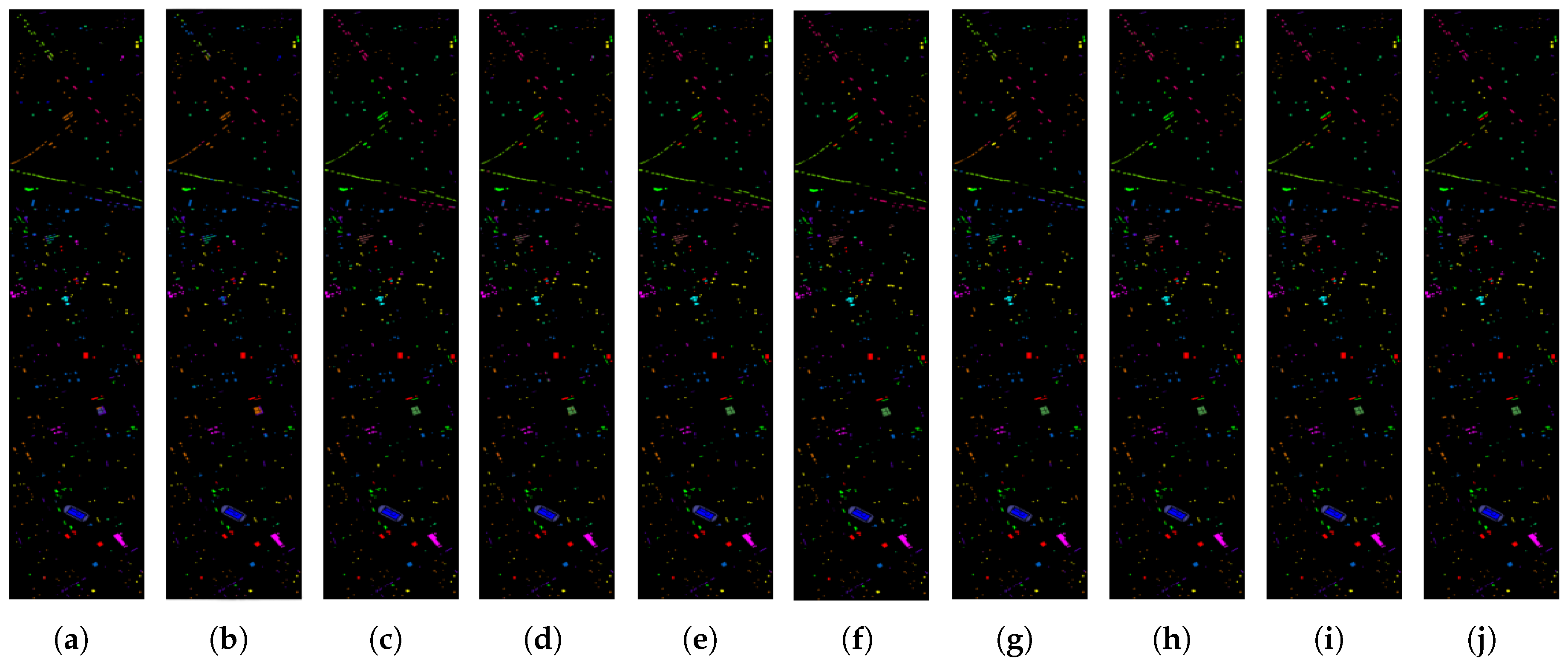
Figure 9. Classification maps of the QUH-Tangdaowan dataset: (a) HybridSN; (b) A2S2K; (c) GMA_Net; (d) SpectralFormer; (e) GSC-ViT; (f) MHCFormer; (g) 3DSS-Mamba; (h) MambaHSI; (i) HSI-MFormer; (j) FreqMamba.
Remotesensing 17 03749 g009
Figure 10. Classification maps of the QUH-Qingyun dataset: (a) HybridSN; (b) A2S2K; (c) GMA_Net; (d) SpectralFormer; (e) GSC-ViT; (f) MHCFormer; (g) 3DSS-Mamba; (h) MambaHSI; (i) HSI-MFormer; (j) FreqMamba.
Remotesensing 17 03749 g010
Figure 11. Classification maps of the QUH-Pingan dataset: (a) HybridSN; (b) A2S2K; (c) GMA_Net; (d) SpectralFormer; (e) GSC-ViT; (f) MHCFormer; (g) 3DSS-Mamba; (h) MambaHSI; (i) HSI-MFormer; (j) FreqMamba.
Remotesensing 17 03749 g011
Figure 12. Classification maps of the Houston dataset: (a) HybridSN; (b) A2S2K; (c) GMA_Net; (d) SpectralFormer; (e) GSC-ViT; (f) MHCFormer; (g) 3DSS-Mamba; (h) MambaHSI; (i) HSI-MFormer; (j) FreqMamba.
Remotesensing 17 03749 g012
Figure 13. Classification maps of the PU dataset: (a) HybridSN; (b) A2S2K; (c) GMA_Net; (d) SpectralFormer; (e) GSC-ViT; (f) MHCFormer; (g) 3DSS-Mamba; (h) MambaHSI; (i) HSI-MFormer; (j) FreqMamba.
Remotesensing 17 03749 g013
Table 1. Number of training, validation, and test ground truth data in the QUH-Tangdaowan dataset.
No.ClassTrainValitionTestTotal
C1Rubber track1292258521,97225,849
C2Flaggingv2778555547,22055,553
C3Sandy1702340428,93134,037
C4Asphalt3035606951,58660,690
C5Boardwalk9318615831862
C6Rocky shallows1856371231,55737,125
C7Grassland706141312,00814,127
C8Bulrush3204640954,47464,087
C9Gravel road1535306926,09130,695
C10Ligustrum vicaryi8917815161783
C11Coniferous pine1062212418,05021,236
C12Spiraea3875636749
C13Bare soil8416914331686
C14Buxus sinica4489753886
C15Photinia serrulata701140211,91714,020
C16Populus704514,090119,769140,904
C17Ulmus pumila L49098083329802
C18Seawater2114422735,93442,275
Total 57,046114,093969,7981,140,937
Table 2. Number of training, validation, and test ground truth data in the QUH-Qingyun dataset.
No.ClassTrainValitionTestTotal
C1Trees13,90727,815236,428278,150
C2Concrete building897617,951152,585179,512
C3Car689137811,71613,783
C4Ironhide building48897783029767
C5Plastic playground10,88721,773185,075217,735
C6Asphalt road12,79725,595217,554255,946
Total 47,74495,489811,660954,893
Table 3. Number of training, validation, and test ground truth data in the QUH-Pingan dataset.
No.ClassTrainValitionTestTotal
C1Ship2447489341,59548,935
C2Seawater28,90557,811491,397578,113
C3Trees41783570938345
C4Concrete structure building4449889775,62788,973
C5Floating pier1038207617,64520,759
C6Brick houses704140911,97314,086
C7Steel houses700139911,89213,991
C8Wharf construction land4156831170,64683,113
C9Car40581168928108
C10Road13,82527,651235,038276,514
Total 57,046114,093969,7981,140,937
Table 4. Number of training, validation, and test ground truth data in the Houston2013 dataset.
No.ClassTrainValitionTestTotal
C1Healthy grass6312510631251
C2Stressed grass6312510661254
C3Synthetic grass3570592697
C4Trees6212410581244
C5Soil6212410561242
C6Water1633276325
C7Residential6312710781268
C8Commercial6212410581244
C9Road6312510641252
C10Highway6112310431227
C11Railway6212310501235
C12Parking lot 16212310481233
C13Parking lot 22347399469
C14Tennis court2143364428
C15Running track3366561660
Total 751150212,77615,029
Table 5. Number of training, validation, and test ground truth data in the PU dataset.
No.ClassTrainValitionTestTotal
C1Asphalt13266358366631
C2Meadows373186516,41118,649
C3Gravel4221018472099
C4Trees6130626973064
C5Painted metal sheets2713411841345
C6Bare soil10050344265029
C7Bitumen2713311701330
C8Self-locking bricks7436832403682
C9Shadows1995833947
Total 855427737,64442,776
Table 6. Classification results of each model on the dataset QUH-Tangdaowan.
No.HybridSNA2S2KGMA_NetSpectralFormerGSC-ViTMHCFormer3DSS-MambaMambaHSIHSI-MFormerFreqMamba
C1 97.98 ± 1.43 99.07 ± 0.72 98.50 ± 0.54 98.88 ± 0.95 98.22 ± 0.42 94.16 ± 1.23 99.30 ± 0.15 99.02 ± 0.33 89.01 ± 0.42 99 . 41 ± 0 . 58
C2 94.11 ± 0.95 99 . 72 ± 0 . 70 96.09 ± 0.67 96.38 ± 1.41 98.17 ± 1.25 91.99 ± 3.78 95.00 ± 2.62 90.69 ± 0.65 93.05 ± 1.80 98.61 ± 0.70
C3 83.46 ± 2.58 89.46 ± 1.82 85.35 ± 1.23 95.21 ± 1.42 89.57 ± 1.56 92.12 ± 2.56 89.70 ± 0.44 88.65 ± 2.23 87.14 ± 4.78 97 . 26 ± 1 . 52
C4 93.21 ± 2.37 93.73 ± 2.06 98.07 ± 4.61 95.40 ± 1.81 97.91 ± 0.89 95.73 ± 4.12 96.99 ± 0.89 95.75 ± 0.60 97.42 ± 0.23 99 . 42 ± 0 . 74
C5 90.40 ± 0.86 96.16 ± 0.66 99 . 05 ± 0 . 88 86.30 ± 6.42 98.40 ± 2.35 86.27 ± 1.89 98.54 ± 1.49 67.72 ± 5.51 91.78 ± 1.24 98.15 ± 1.97
C6 88.59 ± 1.27 98.09 ± 1.49 95.69 ± 1.67 96.45 ± 2.28 95.46 ± 1.94 97.92 ± 3.21 92.13 ± 1.52 78.56 ± 2.65 98 . 72 ± 0 . 63 89.99 ± 2.74
C7 81.62 ± 3.15 88.62 ± 5.45 78.89 ± 5.41 91.26 ± 2.36 82.71 ± 3.20 96 . 09 ± 4 . 76 73.62 ± 0.63 77.26 ± 1.86 91.10 ± 1.06 94.78 ± 0.81
C8 98.01 ± 1.70 98.01 ± 1.70 98.02 ± 2.34 92.90 ± 1.02 98.20 ± 1.57 89.66 ± 2.05 96.41 ± 1.18 95.52 ± 0.94 96.02 ± 1.17 98 . 41 ± 1 . 03
C9 92.08 ± 0.73 94.50 ± 0.73 45.27 ± 21.11 96.23 ± 0.57 98.47 ± 0.55 94.17 ± 1.54 97.54 ± 0.49 74.81 ± 3.48 97.48 ± 0.74 99 . 03 ± 0 . 77
C10 97.28 ± 0.68 98 . 28 ± 2 . 15 42.46 ± 6.14 84.26 ± 3.28 96.68 ± 1.97 83.81 ± 3.90 92.78 ± 2.29 93.78 ± 2.53 85.06 ± 0.11 94.51 ± 1.98
C11 77.78 ± 1.33 91.78 ± 2.66 74.92 ± 7.94 82.71 ± 2.31 88.46 ± 1.87 92.92 ± 4.37 67.47 ± 2.96 64.38 ± 5.96 80.33 ± 3.23 95 . 32 ± 1 . 25
C12 91.73 ± 1.61 89.91 ± 5.05 64.02 ± 13.16 90.07 ± 1.63 89.51 ± 6.43 85.47 ± 2.68 88.56 ± 5.17 91.67 ± 1.72 85.19 ± 3.41 98 . 02 ± 0 . 75
C13 95.48 ± 3.13 97.03 ± 2.92 82.90 ± 6.64 85.35 ± 3.64 93.14 ± 0.61 84.69 ± 1.32 89.46 ± 3.63 91.52 ± 2.67 89.69 ± 2.10 98 . 93 ± 0 . 46
C14 92.91 ± 1.42 91.93 ± 5.77 79.73 ± 5.13 93.72 ± 3.26 88.63 ± 3.59 89.54 ± 3.51 90.97 ± 3.69 83.67 ± 3.62 97 . 07 ± 0 . 52 96.53 ± 1.29
C15 98.03 ± 1.32 94.69 ± 0.97 77.64 ± 0.64 97.19 ± 0.94 95.61 ± 1.19 98.53 ± 4.92 89.84 ± 1.19 88.78 ± 1.08 98 . 64 ± 0 . 24 87.53 ± 0.93
C16 92.33 ± 1.50 96.33 ± 1.50 89.92 ± 4.47 94.45 ± 3.91 96 . 48 ± 3 . 37 93.08 ± 2.17 90.57 ± 3.20 88.45 ± 1.45 95.78 ± 0.11 93.65 ± 2.71
C17 90.14 ± 2.32 98 . 31 ± 0 . 92 86.00 ± 5.71 93.68 ± 6.15 87.39 ± 4.17 91.32 ± 1.69 96.11 ± 2.29 87.27 ± 3.40 96.38 ± 2.34 96.63 ± 2.81
C18 95.67 ± 1.94 97.87 ± 2.31 95.72 ± 1.35 92.21 ± 2.63 98 . 65 ± 0 . 94 81.97 ± 3.45 93.57 ± 2.62 95.93 ± 2.34 93.35 ± 1.59 98.05 ± 1.37
OA (%) 92.73 ± 0.73 91.34 ± 0.63 90.46 ± 1.24 94.55 ± 0.20 95.67 ± 0.86 91.35 ± 1.02 93.21 ± 0.54 88.93 ± 0.53 95.03 ± 0.83 96 . 48 ± 0 . 51
AA (%) 89.31 ± 0.97 86.41 ± 1.16 71.09 ± 1.98 91.66 ± 0.81 94.96 ± 1.16 88.15 ± 0.96 89.27 ± 0.79 85.84 ± 0.97 91.41 ± 0.79 93 . 41 ± 0 . 84
κ × 100 91.42 ± 0.79 90.73 ± 0.84 88.86 ± 1.36 92.26 ± 0.25 94.85 ± 0.98 81.73 ± 1.06 92.46 ± 0.72 86.39 ± 0.61 92.81 ± 0.73 95 . 98 ± 0 . 66
Table 7. Classification results of each model on the dataset QUH-Qingyun.
No.HybridSNA2S2KGMA_NetSpectralFormerGSC-ViTMHCFormer3DSS-MambaMambaHSIHSI-MFormerFreqMamba
C1 96.81 ± 3.02 90.09 ± 4.72 93.77 ± 3.34 89.21 ± 4.69 95.94 ± 1.85 95.76 ± 1.23 93.52 ± 1.67 92.78 ± 2.31 92.16 ± 0.67 97 . 12 ± 0 . 74
C2 91.89 ± 1.79 89.24 ± 3.58 97 . 93 ± 0 . 26 93.58 ± 0.34 96.57 ± 0.81 95.46 ± 0.82 94.48 ± 1.03 87.15 ± 0.66 93.39 ± 2.22 97.61 ± 0.36
C3 75.59 ± 1.09 72.63 ± 3.46 85.07 ± 4.87 86.54 ± 1.27 80.64 ± 2.29 91 . 99 ± 1 . 69 83.89 ± 8.86 72.81 ± 4.94 74.28 ± 5.23 79.24 ± 1.38
C4 95.75 ± 2.89 88.98 ± 1.19 98.06 ± 0.61 96.86 ± 0.14 90.60 ± 0.90 98.70 ± 3.72 98 . 86 ± 0 . 85 97.84 ± 0.98 91.50 ± 1.31 98.27 ± 1.12
C5 95.18 ± 2.83 97.97 ± 1.99 98.03 ± 1.87 91.85 ± 2.19 95.53 ± 0.33 96.03 ± 0.23 96.55 ± 0.20 96.68 ± 0.29 99 . 10 ± 0 . 50 97.72 ± 0.91
C6 89.02 ± 7.63 85.74 ± 2.74 90.53 ± 0.78 95 . 03 ± 0 . 29 89.52 ± 1.46 91.92 ± 5.47 91.63 ± 1.65 76.11 ± 1.80 89.94 ± 3.01 92.61 ± 0.71
OA (%) 90.51 ± 1.03 87.48 ± 1.13 94.27 ± 0.43 90.73 ± 0.64 94.53 ± 0.32 94.94 ± 1.45 93.78 ± 0.83 86.38 ± 0.67 90.28 ± 1.40 95 . 58 ± 0 . 31
AA (%) 84.93 ± 2.13 86.75 ± 1.15 86.73 ± 1.49 86.08 ± 2.77 91.12 ± 0.83 88.94 ± 1.32 87.36 ± 0.92 80.78 ± 0.98 85.87 ± 1.77 91 . 71 ± 0 . 52
κ × 100 88.05 ± 1.50 87.67 ± 1.14 92.51 ± 0.58 87.63 ± 0.51 93.76 ± 0.44 92.93 ± 2.25 91.75 ± 1.11 82.52 ± 0.91 87.01 ± 1.91 94 . 14 ± 0 . 40
Table 8. Classification results of each model on the dataset QUH-Pingan.
No.HybridSNA2S2KGMA_NetSpectralFormerGSC-ViTMHCFormer3DSS-MambaMambaHSIHSI-MFormerFreqMamba
C1 79.15 ± 4.88 85.07 ± 6.37 77.69 ± 2.77 91.07 ± 5.33 84.96 ± 0.96 81.71 ± 1.13 89.22 ± 4.95 81.75 ± 1.57 92.88 ± 1.33 93 . 23 ± 1 . 70
C2 99.34 ± 4.64 89.16 ± 6.14 99.30 ± 3.05 98.80 ± 6.03 99.46 ± 1.19 99.58 ± 0.66 98.33 ± 5.36 96.00 ± 1.74 99 . 61 ± 0 . 29 98.88 ± 0.89
C3 93.20 ± 0.22 88.34 ± 5.49 95.78 ± 1.30 94.86 ± 0.19 98.15 ± 0.18 94.52 ± 0.48 94.90 ± 2.86 88.71 ± 0.84 97.62 ± 0.76 98 . 77 ± 0 . 48
C4 72.75 ± 4.12 83.22 ± 3.42 83.76 ± 2.35 94.31 ± 2.26 87.45 ± 0.87 93.77 ± 0.33 86.90 ± 3.33 88.69 ± 1.49 98 . 12 ± 0 . 83 92.18 ± 1.36
C5 78.79 ± 2.85 77.09 ± 2.55 77.26 ± 3.76 89.23 ± 0.76 88.11 ± 0.98 78.99 ± 1.01 78.58 ± 1.97 76.67 ± 1.80 98 . 58 ± 0 . 33 95.54 ± 0.71
C6 96.21 ± 5.37 86.29 ± 8.85 96.77 ± 0.64 95.89 ± 0.20 97.22 ± 1.09 85.57 ± 1.03 89.70 ± 0.00 86.18 ± 0.35 89.51 ± 1.00 97 . 77 ± 1 . 19
C7 94.76 ± 14.77 86.22 ± 3.43 97 . 45 ± 3 . 76 94.02 ± 3.10 96.49 ± 2.79 89.74 ± 4.47 96.01 ± 5.39 96.73 ± 2.58 89.14 ± 0.67 95.87 ± 3.83
C8 89.50 ± 5.55 86.33 ± 5.30 91.63 ± 3.72 83.59 ± 1.05 91.01 ± 6.87 85.28 ± 2.82 84.69 ± 5.04 70.95 ± 1.48 88.35 ± 0.90 93 . 40 ± 0 . 57
C9 68.51 ± 6.61 83.54 ± 4.86 82.86 ± 3.31 94 . 04 ± 2 . 34 88.75 ± 1.30 84.38 ± 7.91 79.07 ± 4.99 65.92 ± 3.61 86.29 ± 3.97 90.83 ± 4.11
C10 95.18 ± 15.09 78.65 ± 5.58 91.85 ± 4.85 92.76 ± 4.56 96.70 ± 6.10 93.24 ± 3.24 94.66 ± 5.96 94.37 ± 1.49 91.45 ± 2.12 98 . 88 ± 0 . 96
OA (%) 93.59 ± 1.04 87.65 ± 1.62 94.37 ± 1.32 91.48 ± 0.45 96.20 ± 1.67 92.39 ± 1.19 94.53 ± 1.22 91.60 ± 0.93 93.52 ± 0.71 97 . 47 ± 0 . 87
AA (%) 84.61 ± 0.89 84.43 ± 1.66 85.33 ± 1.11 89.49 ± 0.37 89.88 ± 1.37 89.50 ± 1.07 86.06 ± 0.87 79.35 ± 0.62 87.31 ± 0.84 93 . 52 ± 0 . 63
κ × 100 90.46 ± 1.12 86.50 ± 1.76 91.60 ± 1.46 90.06 ± 0.48 94.35 ± 1.80 92.45 ± 1.28 91.81 ± 1.32 87.34 ± 0.88 90.98 ± 0.69 96 . 22 ± 0 . 94
Table 9. Classification results of each model on the dataset Htouston2013.
No.HybridSNA2S2KGMA_NetSpectralFormerGSC-ViTMHCFormer3DSS-MambaMambaHSIHSI-MFormerFreqMamba
C1 96.65 ± 4.88 88.99 ± 6.37 91.39 ± 2.77 94.07 ± 5.33 97 . 93 ± 0 . 96 85.80 ± 1.13 92.41 ± 4.95 96.09 ± 1.57 95.90 ± 1.33 97.36 ± 1.70
C2 91.56 ± 4.64 90.39 ± 6.14 93.83 ± 3.05 92.80 ± 6.03 97.75 ± 1.19 99 . 34 ± 0 . 66 93.51 ± 5.36 98.45 ± 1.74 95.57 ± 2.09 98.57 ± 1.89
C3 99 . 91 ± 0 . 22 94.15 ± 5.49 92.51 ± 1.30 99.86 ± 0.19 99.82 ± 0.18 99.52 ± 0.48 96.48 ± 2.86 99.35 ± 0.84 99.19 ± 0.76 99.52 ± 0.48
C4 94.00 ± 4.12 93.53 ± 3.42 89.86 ± 2.35 98.31 ± 2.26 96.89 ± 0.87 93.77 ± 0.33 96.66 ± 3.33 97.93 ± 1.49 94.46 ± 0.83 98 . 57 ± 1 . 36
C5 98.46 ± 2.85 95.28 ± 2.55 94.88 ± 3.76 99.23 ± 0.76 96.52 ± 0.98 98.99 ± 1.01 97.39 ± 1.97 98.86 ± 1.80 98.43 ± 0.33 99 . 29 ± 0 . 71
C6 94.72 ± 5.37 87.78 ± 8.85 98.25 ± 0.64 99.89 ± 0.20 98.91 ± 1.09 85.57 ± 1.03 100 . 00 ± 0 . 00 98.97 ± 0.35 95.45 ± 1.00 97.75 ± 1.19
C7 78.32 ± 14.77 84.15 ± 3.43 89.76 ± 3.76 94.02 ± 3.10 93.88 ± 2.79 89.74 ± 4.47 89.78 ± 5.39 95.01 ± 2.58 89.75 ± 0.67 95 . 05 ± 3 . 83
C8 73.44 ± 5.55 87.32 ± 5.30 93.96 ± 3.72 97.59 ± 1.05 88.02 ± 6.87 65.28 ± 2.82 92.44 ± 5.04 97.19 ± 1.48 95.48 ± 0.90 98 . 47 ± 0 . 57
C9 77.84 ± 6.61 86.04 ± 4.86 89.70 ± 3.31 94.04 ± 2.34 86.00 ± 1.30 84.38 ± 7.91 92.96 ± 4.99 95 . 57 ± 3 . 61 90.70 ± 3.97 94.77 ± 4.11
C10 66.94 ± 15.09 78.65 ± 5.58 86.77 ± 4.85 92.76 ± 4.56 81.70 ± 6.10 83.24 ± 3.24 85.27 ± 5.96 94.60 ± 1.49 91.45 ± 2.12 96 . 60 ± 0 . 96
C11 78.96 ± 7.09 78.87 ± 6.76 92.68 ± 4.58 92.85 ± 4.16 91.06 ± 4.50 88.75 ± 7.48 92.43 ± 2.95 94.60 ± 1.49 88.89 ± 2.00 96 . 53 ± 3 . 04
C12 90.03 ± 6.59 81.64 ± 5.63 87.62 ± 3.96 92.85 ± 2.67 87.51 ± 5.43 96 . 76 ± 1 . 35 94.21 ± 4.33 93.66 ± 4.53 91.28 ± 3.46 95.46 ± 1.76
C13 93.99 ± 1.33 88.08 ± 5.75 94.24 ± 3.85 96.69 ± 2.45 82.91 ± 8.64 90.60 ± 3.73 91.23 ± 6.92 94.63 ± 2.73 97 . 42 ± 2 . 08 97.27 ± 0.94
C14 99.95 ± 0.15 85.85 ± 8.26 92.98 ± 5.08 99.60 ± 0.44 97.44 ± 1.27 99.61 ± 0.39 96.02 ± 3.44 99.04 ± 0.81 98.60 ± 0.91 100 . 00 ± 0 . 00
C15 99.88 ± 0.26 95.54 ± 3.46 95.62 ± 2.39 99.16 ± 0.93 92.10 ± 2.71 99 . 75 ± 0 . 25 96.12 ± 2.37 99.27 ± 1.22 93.62 ± 4.61 98.60 ± 1.10
OA (%) 86.92 ± 1.04 86.48 ± 1.62 87.19 ± 1.32 91.94 ± 1.67 95.48 ± 0.45 91.39 ± 1.19 94.40 ± 1.22 95.77 ± 0.93 93.52 ± 0.23 96 . 54 ± 0 . 87
AA (%) 88.98 ± 0.89 87.75 ± 1.66 88.14 ± 1.11 90.95 ± 1.37 95.49 ± 0.37 90.50 ± 1.07 95.03 ± 0.87 95.57 ± 0.62 93.31 ± 0.29 96 . 16 ± 0 . 63
κ × 100 85.85 ± 1.12 85.77 ± 1.76 87.66 ± 1.46 91.28 ± 1.48 95.06 ± 0.50 90.45 ± 1.28 94.71 ± 1.32 95.33 ± 0.88 92.98 ± 0.23 96 . 03 ± 0 . 94
Table 10. Classification results of each model on the dataset PU.
No.HybridSNA2S2KGMA_NetSpectralFormerGSC-ViTMHCFormer3DSS-MambaMambaHSIHSI-MFormerFreqMamba
C1 58.81 ± 3.02 62.09 ± 4.72 92.77 ± 3.34 89.21 ± 6.69 75.94 ± 1.85 81.76 ± 2.23 98 . 52 ± 1 . 67 84.78 ± 2.31 92.16 ± 0.67 96.58 ± 0.74
C2 96.89 ± 1.79 90.24 ± 3.58 98.93 ± 0.26 93.58 ± 0.34 87.57 ± 0.81 97.46 ± 3.22 97.48 ± 1.03 97.15 ± 0.66 93.39 ± 2.22 99 . 25 ± 0 . 36
C3 70.59 ± 16.09 42.63 ± 3.46 89.07 ± 4.87 97 . 54 ± 1 . 27 80.64 ± 2.29 75.99 ± 37.69 83.89 ± 8.86 68.81 ± 4.94 74.28 ± 5.23 97.18 ± 1.38
C4 85.75 ± 2.89 88.88 ± 1.19 98.06 ± 0.61 96.86 ± 0.14 98.60 ± 0.90 98 . 70 ± 3 . 72 96.86 ± 0.85 97.84 ± 0.98 91.50 ± 1.31 97.51 ± 1.12
C5 99.18 ± 0.83 82.97 ± 18.99 98.03 ± 1.87 91.85 ± 2.19 95.53 ± 0.33 96.03 ± 0.23 99.55 ± 0.20 99 . 68 ± 0 . 29 99.10 ± 0.50 99.24 ± 0.91
C6 49.02 ± 7.63 65.74 ± 8.74 96.53 ± 0.78 95.03 ± 0.29 82.52 ± 1.46 91.92 ± 5.47 96.68 ± 1.65 95.11 ± 1.80 89.94 ± 3.01 98 . 52 ± 0 . 71
C7 94.46 ± 1.82 39.17 ± 3.44 80.86 ± 9.98 42.46 ± 43.34 76.61 ± 6.00 82.56 ± 4.38 87.42 ± 7.77 64.82 ± 7.47 74.37 ± 2.50 98 . 03 ± 1 . 30
C8 76.42 ± 9.68 38.73 ± 3.82 89.48 ± 2.87 90.03 ± 1.85 78.97 ± 3.94 74.25 ± 3.21 90.34 ± 2.18 79.27 ± 2.42 80.32 ± 1.95 96 . 08 ± 2 . 41
C9 97.23 ± 2.36 77.59 ± 13.21 99 . 21 ± 0 . 65 97.15 ± 1.24 90.81 ± 2.08 97.48 ± 1.68 96.18 ± 1.35 97.11 ± 0.47 93.17 ± 1.74 95.98 ± 1.81
OA (%) 81.51 ± 1.03 74.48 ± 2.13 93.87 ± 0.43 90.73 ± 0.29 94.53 ± 0.32 90.94 ± 1.45 95.37 ± 0.83 93.38 ± 0.67 94.28 ± 0.61 96 . 48 ± 0 . 31
AA (%) 80.93 ± 2.13 60.75 ± 4.15 90.73 ± 1.49 86.08 ± 2.77 93.12 ± 0.83 93.94 ± 1.32 94.00 ± 0.92 92.78 ± 0.98 94.87 ± 0.77 95 . 17 ± 0 . 52
κ × 100 75.05 ± 1.50 65.67 ± 3.14 92.51 ± 0.558 87.63 ± 0.51 93.76 ± 0.44 87.93 ± 2.25 93.85 ± 1.11 93.52 ± 0.91 94.01 ± 0.71 95 . 03 ± 0 . 40
Table 11. Model complexity comparison across different datasets.
DatasetMetricHybridSNA2S2KGMA_NetSpectralFormerGSC-ViTMHCFormer3DSS-MambaMambaHSIHSI-MFormerFreqMamba
TangdaowanParam (M)3.9910.3331.6150.3130.1713.3910.1280.1280.2970.308
FLOPs (M)431.068225.45430.20931.9796.161274.9742.2826.846148.5428.292
PinganParam (M)3.9910.3331.6110.3130.1713.3910.1240.1280.2970.273
FLOPs (M)431.068225.45430.20531.9796.160274.9742.2786.84674.2718.258
QingyunParam (M)3.9910.3331.6090.3130.1713.3910.1220.1280.2970.256
FLOPs (M)431.068225.45430.20331.9796.160274.9742.2766.84674.2718.241
Houston2013Param (M)3.4010.2831.5010.2380.1672.8000.0240.1270.2970.107
FLOPs (M)350.101183.77223.19024.41411.274225.91313.9262.28074.2711.027
PUParam (M)2.6450.2211.3680.1840.1782.0440.0240.1240.2970.082
FLOPs (M)246.351131.67130.81231.7349.924326.1213.9622.27774.2711.001
Table 12. The ablation experiment results of the FMDC module.
 OA (%)AA (%) κ × 100
Complete Model96.1795.5595.65
Ordinary 3DCNN92.92 (↓3.25%)89.97 (↓5.58%)90.63 (↓5.02%)
Remove Frequency Domain88.24 (↓7.93%)87.57 (↓7.98%)88.72 (↓6.93%)
Remove FMDC81.92 (↓14.25%)80.97 (↓14.58%)80.25 (↓15.40%)
Table 13. The ablation experimental results of different group sizes in the ViT branch.
Group_SizeOA (%)AA(%) κ × 100
294.8190.0394.08
396.1795.5595.65
496.4893.4195.98
694.5592.4393.79
1293.5689.9292.62
Table 14. The results of the ablation experiment on Mamba branches.
ModelOA (%)AA(%) κ × 100
Complete Model96.1795.5595.65
Remove Mamba94.47 (↓1.70%)85.97 (↓9.58%)93.68 (↓1.97%)
Table 15. Results obtained with different frequency-aware methods.
 OA (%)AA(%) κ × 100
Complete Model96.1795.5595.65
Average Pooling90.04 (↓6.13)88.95 (↓6.60)89.64 (↓6.01)
Discrete Cosine Transform91.34 (↓4.83)90.94 (↓4.61)91.07 (↓4.58)
Fourier Transform93.26 (↓2.91)91.48 (↓4.07)92.88 (↓2.77)
Gabor Filter91.54 (↓4.63)89.35 (↓6.21)90.91 (↓4.74)
Disclaimer/Publisher’s Note: The statements, opinions and data contained in all publications are solely those of the individual author(s) and contributor(s) and not of MDPI and/or the editor(s). MDPI and/or the editor(s) disclaim responsibility for any injury to people or property resulting from any ideas, methods, instructions or products referred to in the content.