Figure 1.
Overall structure of proposed AFGNet. First, the PCA algorithm is used to remove redundant bands. Then, the proposed AFEM module is constructed to distinguish the primary features from the secondary features. Next, the proposed GWF2 module is designed to extract local features with the assistance of global features. Finally, the proposed MHCA module is utilized to extract global features and complete classification prediction.
Figure 2.
Structure of AFEM. First, the central pixel is extracted from the input spectral cube. After that, the similarity matrix between the surrounding pixels and the central pixel is obtained using cosine similarity. Next, the similarity matrix is split into primary and secondary features by a preset threshold and multiplied with the adaptive coefficient. Finally, the attention map is merged and the original feature map is weighted.
Figure 3.
Structure of MHCA. The input sequence is divided into two branches. First, the first branch uses maximum pooling and mean pooling to obtain the attention map. Then, the second branch maps the Q branch and the K.V branch independently and uses scaled dot product attention to obtain the weighted feature map. Finally, the attention map of the first branch is used to re-weight the result of the second branch to obtain the final feature map.
Figure 4.
Impact of different patch sizes and learning rates on classification performance, (a–e): Indian Pines, Pavia University, Houston 2013, Longkou, and LaoYuHe. For the IP and UP datasets, the patch size was set to 13 × 13, and the learning rate was set to 1 ×10⁻³. For the HT dataset, the patch size was set to 13 × 13, and the learning rate was set to 5 ×10⁻⁴. For the LK dataset, the patch size was set to 15 × 15, and the learning rate was set to 5 ×10⁻³. For the LYH dataset, the patch size was set to 15 × 15, and the learning rate was set to 5 ×10⁻⁴.
Figure 5.
Ablation for GWF2. Fspe and Fspa represent spectral feature fusion and spatial feature fusion, respectively. Markings in the upper left corner represent, from top to bottom, not using Fspe and Fspa, only using Fspa, only using Fspe, and complete GWF2 module (including Fspe and Fspa).
Figure 5.
Ablation for GWF2. Fspe and Fspa represent spectral feature fusion and spatial feature fusion, respectively. Markings in the upper left corner represent, from top to bottom, not using Fspe and Fspa, only using Fspa, only using Fspe, and complete GWF2 module (including Fspe and Fspa).
Figure 6.
Impact of different patch sizes and learning rates on classification performance, (a–e): Indian Pines, Pavia University, Houston 2013, Longkou, and LaoYuHe. Alpha and beta represent adaptive scaling coefficients of primary and secondary features, respectively.
Figure 6.
Impact of different patch sizes and learning rates on classification performance, (a–e): Indian Pines, Pavia University, Houston 2013, Longkou, and LaoYuHe. Alpha and beta represent adaptive scaling coefficients of primary and secondary features, respectively.
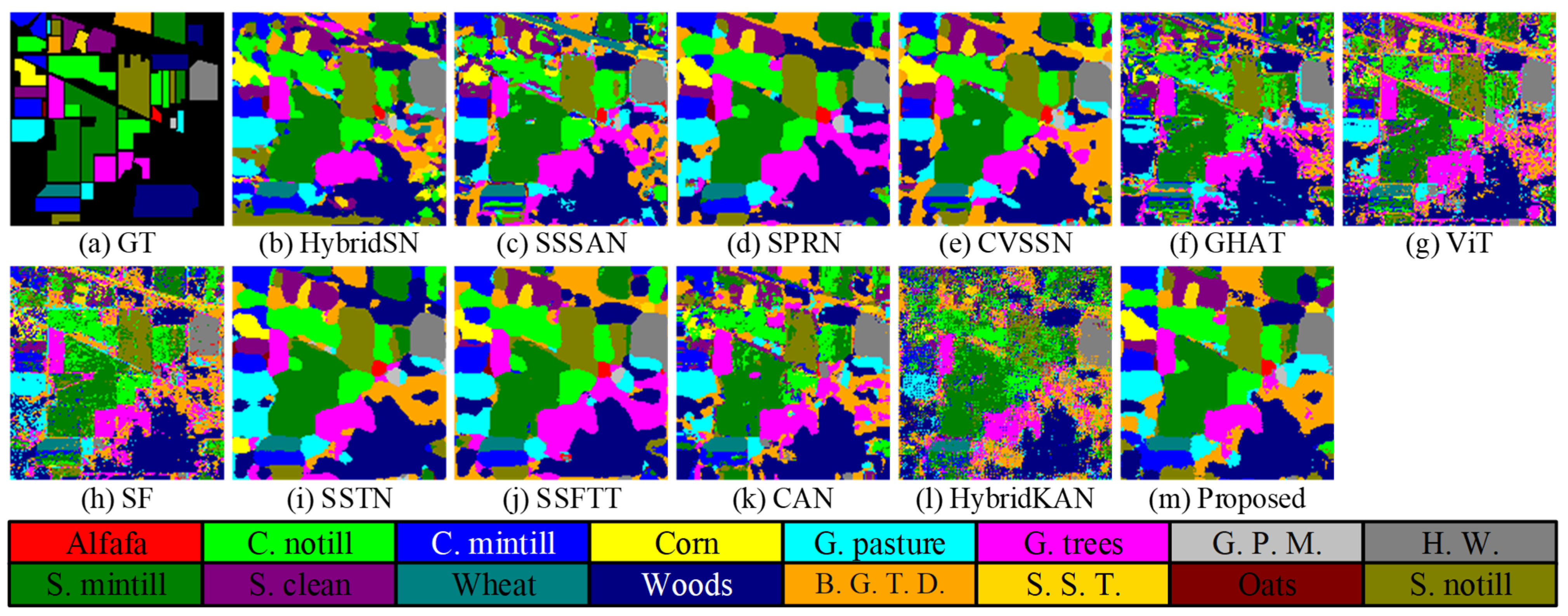
Figure 7.
Classification maps obtained by different methods on the IP dataset, (a–m): Ground Truth, HybridSN, SSSAN, SPRN, CVSSN, GHAT, SF, SSTN, SSFTT, AFGNet, respectively.
Figure 7.
Classification maps obtained by different methods on the IP dataset, (a–m): Ground Truth, HybridSN, SSSAN, SPRN, CVSSN, GHAT, SF, SSTN, SSFTT, AFGNet, respectively.
Figure 8.
Classification maps obtained by different methods on the UP dataset, (a–m): Ground Truth, HybridSN, SSSAN, SPRN, CVSSN, GHAT, SF, SSTN, SSFTT, AFGNet, respectively.
Figure 8.
Classification maps obtained by different methods on the UP dataset, (a–m): Ground Truth, HybridSN, SSSAN, SPRN, CVSSN, GHAT, SF, SSTN, SSFTT, AFGNet, respectively.
Figure 9.
Classification maps obtained by different methods on the HT dataset, (a–m): Ground Truth, HybridSN, SSSAN, SPRN, CVSSN, GHAT, SF, SSTN, SSFTT, AFGNet, respectively.
Figure 9.
Classification maps obtained by different methods on the HT dataset, (a–m): Ground Truth, HybridSN, SSSAN, SPRN, CVSSN, GHAT, SF, SSTN, SSFTT, AFGNet, respectively.
Figure 10.
Classification maps obtained by different methods on LK dataset, (a–m): Ground Truth, HybridSN, SSSAN, SPRN, CVSSN, GHAT, SF, SSTN, SSFTT, and AFGNet, respectively.
Figure 10.
Classification maps obtained by different methods on LK dataset, (a–m): Ground Truth, HybridSN, SSSAN, SPRN, CVSSN, GHAT, SF, SSTN, SSFTT, and AFGNet, respectively.
Figure 11.
Classification maps obtained by different methods on LYH dataset, (a–m): Ground Truth, HybridSN, SSSAN, SPRN, CVSSN, GHAT, SF, SSTN, SSFTT, and AFGNet, respectively.
Figure 11.
Classification maps obtained by different methods on LYH dataset, (a–m): Ground Truth, HybridSN, SSSAN, SPRN, CVSSN, GHAT, SF, SSTN, SSFTT, and AFGNet, respectively.
Figure 12.
Comparison of different sample proportions; (a–e) IP, UP, HT, LK, and LYH datasets, respectively.
Figure 12.
Comparison of different sample proportions; (a–e) IP, UP, HT, LK, and LYH datasets, respectively.
Figure 13.
t-SNE visualization results obtained by different methods on IP dataset (a–d): SPRN, SSTN, SSFTT, Proposed.
Figure 13.
t-SNE visualization results obtained by different methods on IP dataset (a–d): SPRN, SSTN, SSFTT, Proposed.
Figure 14.
t-SNE visualization results obtained by different methods on UP dataset (a–d): SPRN, SSTN, SSFTT, Proposed.
Figure 14.
t-SNE visualization results obtained by different methods on UP dataset (a–d): SPRN, SSTN, SSFTT, Proposed.
Figure 15.
Heat map visualization of features obtained by model at different stages on UP dataset. Compared with the blue area, the red area means that the model pays more attention to this area. (a) Baseline. (b) AFEM. (c) AFEM + GWF2. (d) AFGNet.
Figure 15.
Heat map visualization of features obtained by model at different stages on UP dataset. Compared with the blue area, the red area means that the model pays more attention to this area. (a) Baseline. (b) AFEM. (c) AFEM + GWF2. (d) AFGNet.
Figure 16.
Impact of different proportions of Gaussian noise on each method on UP dataset: SPRN, SSTN, SSFTT, Proposed.
Figure 16.
Impact of different proportions of Gaussian noise on each method on UP dataset: SPRN, SSTN, SSFTT, Proposed.
Table 1.
Training and test samples numbers for Indian Pines, Pavia University, and Houston 2013.
Table 1.
Training and test samples numbers for Indian Pines, Pavia University, and Houston 2013.
| No | Indian Pines | Pavia University | Houston 2013 |
|---|
| Class Name | Training | Test | Class Name | Training | Test | Class Name | Training | Test |
|---|
| 1 | Alfafa | 2 | 44 | Asphalt | 86 | 6545 | Healthy Grass | 63 | 1188 |
| 2 | Corn N. | 71 | 1357 | Meadows | 186 | 18,463 | Stressed Grass | 63 | 1191 |
| 3 | Corn M. | 41 | 789 | Gravel | 21 | 2078 | Synthetic Grass | 35 | 662 |
| 4 | Corn | 12 | 225 | Trees | 31 | 3033 | Trees | 62 | 1182 |
| 5 | Grass P. | 24 | 459 | Painted M. S. | 13 | 1332 | Soil | 62 | 1180 |
| 6 | Grass T. | 37 | 693 | Bare soil | 50 | 4979 | Water | 16 | 309 |
| 7 | Grass P. M. | 1 | 27 | Bitumen | 13 | 1317 | Residential | 63 | 1205 |
| 8 | Hay W. | 24 | 454 | S. B. B. | 37 | 3645 | Commerical | 62 | 1182 |
| 9 | Oats | 1 | 19 | Shadows | 10 | 937 | Road | 63 | 1189 |
| 10 | Soybean N. | 49 | 923 | | 427 | 42,349 | Highway | 61 | 1166 |
| 11 | Soybean M. | 123 | 2332 | | | | Railway | 62 | 1173 |
| 12 | Soybean C. | 30 | 563 | | | | Parking Lot 1 | 62 | 1171 |
| 13 | Wheat | 10 | 195 | | | | Parking Lot 2 | 23 | 446 |
| 14 | Woods | 63 | 1202 | | | | Tennis Court | 21 | 407 |
| 15 | B. G. T. D. | 19 | 367 | | | | Running Track | 33 | 627 |
| 16 | S. S. T. | 5 | 88 | | | | | | |
| - | Total | 512 | 9737 | Total | 427 | 42,349 | Total | 751 | 14,278 |
Table 2.
Training and test samples numbers for Longkou and LaoYuHe.
Table 2.
Training and test samples numbers for Longkou and LaoYuHe.
| No | Longkou | LaoYuHe |
|---|
| Class Name | Training | Test | Class Name | Training | Test |
|---|
| 1 | Corn | 69 | 34,442 | Metasequoia | 55 | 5452 |
| 2 | Cotton | 17 | 8357 | Other Tree Species | 29 | 2853 |
| 3 | Sesame | 6 | 3025 | Greenhouse Farmland | 67 | 6599 |
| 4 | Broad-leaf soybean | 126 | 63,086 | Bare Land | 21 | 2135 |
| 5 | Narrow-leaf soybean | 8 | 4143 | Water Bodies | 77 | 7625 |
| 6 | Rice | 24 | 11,830 | Buildings | 24 | 2432 |
| 7 | Water | 134 | 66,922 | Asphalt | 68 | 6735 |
| 8 | Roads and houses | 14 | 7110 | Pitches | 2 | 166 |
| 9 | Mixed weed | 11 | 5218 | | | |
| - | Total | 409 | 204,133 | | 343 | 33,997 |
Table 3.
Ablation experiments. (OA is adopted as evaluation indicator, the optimal performance is bolded).
Table 3.
Ablation experiments. (OA is adopted as evaluation indicator, the optimal performance is bolded).
| Case | Components | Dataset |
|---|
| AFEM | GWF2 | MHCA | IP | UP | HT | LK | LYH |
|---|
| 1 | ✘ | ✔ | ✘ | 97.27 | 97.94 | 98.17 | 97.99 | 96.31 |
| 2 | ✔ | ✔ | ✘ | 97.78 | 98.26 | 98.56 | 98.72 | 96.94 |
| 3 | ✘ | ✔ | ✔ | 97.60 | 98.28 | 98.58 | 98.58 | 96.68 |
| 4 | ✔ | ✔ | ✔ | 98.12 | 98.34 | 98.68 | 98.88 | 97.06 |
Table 4.
Classification performance obtained by different methods for Indian Pines dataset. (The optimal performance of OA, AA, and κ × 100 are bolded, No. 1–16 represents accuracy of each category).
Table 4.
Classification performance obtained by different methods for Indian Pines dataset. (The optimal performance of OA, AA, and κ × 100 are bolded, No. 1–16 represents accuracy of each category).
| No. | HybridSN | SSSAN | SPRN | CVSSN | GHAT | ViT | SF | SSTN | SSFTT | CAN | HybridKAN | Proposed |
|---|
| 1 | 92.10 | 77.97 | 99.75 | 88.63 | 77.92 | 13.99 | 98.57 | 99.53 | 59.77 | 0.93 | 22.80 | 88.40 |
| 2 | 86.65 | 80.38 | 98.03 | 93.06 | 66.72 | 62.28 | 63.99 | 95.04 | 94.75 | 71.08 | 45.83 | 95.88 |
| 3 | 85.37 | 80.70 | 97.29 | 95.93 | 59.67 | 57.82 | 63.53 | 97.51 | 97.13 | 72.98 | 42.75 | 98.25 |
| 4 | 91.35 | 80.72 | 97.48 | 93.56 | 76.48 | 49.53 | 68.07 | 94.79 | 91.64 | 23.01 | 33.53 | 96.80 |
| 5 | 93.33 | 92.96 | 97.30 | 94.82 | 85.23 | 75.51 | 88.37 | 98.08 | 99.82 | 90.94 | 58.72 | 99.85 |
| 6 | 96.62 | 95.24 | 98.20 | 98.13 | 78.21 | 80.26 | 84.10 | 98.91 | 99.24 | 99.19 | 72.81 | 99.49 |
| 7 | 88.00 | 74.26 | 95.65 | 76.07 | 75.19 | 54.42 | 82.99 | 72.89 | 97.40 | 25.60 | 31.39 | 97.78 |
| 8 | 94.09 | 97.15 | 100 | 99.10 | 90.78 | 84.76 | 89.56 | 99.08 | 99.69 | 99.74 | 81.56 | 99.67 |
| 9 | 48.38 | 56.26 | 79.75 | 78.44 | 62.42 | 40.57 | 73.19 | 89.24 | 78.42 | 60.00 | 9.42 | 91.58 |
| 10 | 86.73 | 85.99 | 94.82 | 90.66 | 69.64 | 68.16 | 72.79 | 93.46 | 97.01 | 64.59 | 39.79 | 97.26 |
| 11 | 91.17 | 89.67 | 98.30 | 94.51 | 75.77 | 69.75 | 69.93 | 97.79 | 99.03 | 76.47 | 57.72 | 98.84 |
| 12 | 89.79 | 67.95 | 99.44 | 88.47 | 57.86 | 48.79 | 51.17 | 92.86 | 91.15 | 47.66 | 32.76 | 94.14 |
| 13 | 97.35 | 94.16 | 96.82 | 99.49 | 83.99 | 74.15 | 83.52 | 98.74 | 99.94 | 98.67 | 8089 | 99.79 |
| 14 | 97.78 | 96.16 | 97.23 | 96.87 | 87.66 | 86.08 | 88.99 | 98.42 | 99.17 | 95.01 | 78.35 | 99.95 |
| 15 | 97.45 | 85.28 | 98.52 | 90.22 | 68.57 | 47.16 | 74.73 | 94.96 | 92.99 | 73.19 | 44.25 | 98.26 |
| 16 | 84.09 | 94.69 | 91.06 | 90.47 | 95.23 | 91.87 | 93.94 | 95.46 | 86.47 | 75.51 | 77.20 | 99.89 |
| OA | 91.07 | 87.19 | 97.62 | 94.13 | 74.47 | 68.96 | 73.47 | 96.51 | 97.02 | 76.89 | 56.91 | 98.12 |
| AA | 88.76 | 84.35 | 96.23 | 91.78 | 75.71 | 62.82 | 78.07 | 94.80 | 92.73 | 67.16 | 50.61 | 97.24 |
| κ × 100 | 89.79 | 85.38 | 97.29 | 93.31 | 70.74 | 64.49 | 69.31 | 96.02 | 96.61 | 73.57 | 50.21 | 97.86 |
Table 5.
Classification performance obtained by different methods for Pavia University dataset. (The optimal performance of OA, AA, and κ × 100 are bolded, No. 1–9 represents accuracy of each category).
Table 5.
Classification performance obtained by different methods for Pavia University dataset. (The optimal performance of OA, AA, and κ × 100 are bolded, No. 1–9 represents accuracy of each category).
| No. | HybridSN | SSSAN | SPRN | CVSSN | GHAT | ViT | SF | SSTN | SSFTT | CAN | HybridKAN | Proposed |
|---|
| 1 | 94.77 | 93.35 | 91.17 | 95.66 | 85.35 | 85.36 | 84.34 | 97.88 | 97.20 | 95.12 | 62.93 | 98.21 |
| 2 | 99.16 | 97.34 | 99.67 | 98.61 | 90.52 | 88.51 | 93.81 | 97.97 | 99.92 | 97.86 | 84.47 | 99.98 |
| 3 | 89.73 | 81.99 | 98.08 | 87.96 | 61.52 | 63.20 | 69.77 | 98.13 | 88.33 | 0.00 | 48.13 | 87.08 |
| 4 | 96.11 | 98.52 | 98.68 | 97.52 | 96.53 | 86.71 | 98.80 | 95.99 | 94.08 | 2.47 | 76.91 | 94.88 |
| 5 | 95.68 | 95.49 | 99.95 | 96.64 | 98.40 | 93.74 | 99.05 | 97.94 | 99.45 | 98.80 | 96.61 | 99.90 |
| 6 | 99.58 | 92.68 | 98.61 | 96.74 | 82.45 | 73.68 | 89.02 | 97.96 | 99.73 | 13.47 | 74.20 | 99.60 |
| 7 | 94.91 | 86.31 | 79.10 | 91.41 | 71.73 | 69.24 | 68.49 | 99.12 | 99.93 | 0.00 | 44.08 | 99.97 |
| 8 | 90.99 | 86.74 | 87.26 | 89.73 | 77.56 | 78.45 | 77.43 | 87.30 | 92.93 | 89.08 | 50.15 | 96.90 |
| 9 | 91.55 | 98.96 | 98.98 | 97.59 | 98.01 | 96.26 | 99.69 | 100 | 93.72 | 66.87 | 43.75 | 97.69 |
| OA | 96.68 | 94.12 | 96.19 | 96.20 | 86.67 | 83.65 | 89.12 | 96.87 | 97.73 | 71.42 | 74.07 | 98.34 |
| AA | 94.72 | 92.38 | 94.61 | 94.65 | 84.68 | 81.68 | 86.71 | 96.92 | 96.14 | 51.52 | 64.58 | 97.13 |
| κ × 100 | 95.59 | 92.19 | 94.91 | 94.96 | 82.09 | 78.47 | 85.42 | 95.84 | 97.00 | 58.86 | 64.67 | 97.80 |
Table 6.
Classification performance obtained by different methods for Houston 2013 dataset. (The optimal performance of OA, AA, and κ × 100 are bolded, No. 1–15 represents accuracy of each category).
Table 6.
Classification performance obtained by different methods for Houston 2013 dataset. (The optimal performance of OA, AA, and κ × 100 are bolded, No. 1–15 represents accuracy of each category).
| No. | HybridSN | SSSAN | SPRN | CVSSN | GHAT | ViT | SF | SSTN | SSFTT | CAN | HybridKAN | Proposed |
|---|
| 1 | 96.85 | 94.83 | 97.81 | 96.93 | 94.51 | 91.32 | 96.18 | 90.93 | 97.24 | 85.62 | 92.74 | 99.35 |
| 2 | 98.39 | 95.16 | 97.14 | 97.79 | 96.70 | 94.03 | 97.76 | 96.73 | 99.30 | 83.52 | 96.30 | 99.08 |
| 3 | 98.70 | 96.78 | 99.93 | 98.76 | 97.68 | 99.49 | 96.30 | 99.31 | 99.68 | 84.16 | 99.03 | 100 |
| 4 | 93.27 | 95.02 | 98.29 | 96.21 | 94.93 | 99.02 | 95.29 | 99.27 | 98.79 | 92.03 | 94.38 | 99.78 |
| 5 | 98.85 | 99.24 | 99.02 | 98.97 | 97.69 | 96.64 | 97.82 | 99.48 | 100.00 | 89.25 | 96.56 | 100 |
| 6 | 98.29 | 99.25 | 99.27 | 97.03 | 87.32 | 96.13 | 91.06 | 99.57 | 96.79 | 11.20 | 96.42 | 98.05 |
| 7 | 87.58 | 87.78 | 96.60 | 91.67 | 82.94 | 82.44 | 85.51 | 94.18 | 96.85 | 78.34 | 86.42 | 95.56 |
| 8 | 97.19 | 92.10 | 98.82 | 98.61 | 88.48 | 78.11 | 83.31 | 96.66 | 92.65 | 51.57 | 88.58 | 95.12 |
| 9 | 91.80 | 93.67 | 95.81 | 94.60 | 85.70 | 74.53 | 84.54 | 94.80 | 94.36 | 68.86 | 86.57 | 99.33 |
| 10 | 95.16 | 78.82 | 93.17 | 94.49 | 79.30 | 82.91 | 83.19 | 86.04 | 99.31 | 51.20 | 89.18 | 99.66 |
| 11 | 97.62 | 96.37 | 98.39 | 95.82 | 82.56 | 78.81 | 82.78 | 97.25 | 99.57 | 65.09 | 90.74 | 100 |
| 12 | 97.68 | 85.75 | 92.35 | 95.32 | 83.03 | 76.94 | 89.58 | 94.29 | 98.19 | 47.24 | 87.71 | 99.12 |
| 13 | 93.14 | 90.84 | 96.87 | 95.83 | 85.95 | 62.52 | 87.58 | 90.36 | 94.82 | 0.22 | 91.57 | 93.87 |
| 14 | 99.27 | 87.13 | 100 | 99.03 | 88.24 | 91.83 | 95.42 | 98.40 | 100 | 64.13 | 94.39 | 99.95 |
| 15 | 97.36 | 99.03 | 100 | 97.59 | 95.39 | 96.12 | 95.94 | 97.81 | 99.44 | 70.62 | 96.44 | 100 |
| OA | 95.60 | 92.03 | 97.01 | 96.22 | 88.94 | 86.07 | 90.04 | 95.00 | 97.76 | 68.19 | 91.72 | 98.68 |
| AA | 96.08 | 92.82 | 97.56 | 96.58 | 89.36 | 86.72 | 90.82 | 95.67 | 97.80 | 62.87 | 92.47 | 98.59 |
| κ × 100 | 95.25 | 91.39 | 96.77 | 95.92 | 88.03 | 84.93 | 89.23 | 94.60 | 97.57 | 65.51 | 91.04 | 98.57 |
Table 7.
Classification performance obtained by different methods for Longkou dataset. (The optimal performance of OA, AA, and κ × 100 are bolded, No. 1–9 represents accuracy of each category).
Table 7.
Classification performance obtained by different methods for Longkou dataset. (The optimal performance of OA, AA, and κ × 100 are bolded, No. 1–9 represents accuracy of each category).
| No. | HybridSN | SSSAN | SPRN | CVSSN | GHAT | ViT | SF | SSTN | SSFTT | CAN | HybridKAN | Proposed |
|---|
| 1 | 98.46 | 98.53 | 98.23 | 99.19 | 98.96 | 94.92 | 94.78 | 98.75 | 99.59 | 99.38 | 79.92 | 99.95 |
| 2 | 94.24 | 65.14 | 91.14 | 94.70 | 77.27 | 49.89 | 66.88 | 89.27 | 98.50 | 97.57 | 57.52 | 98.53 |
| 3 | 91.92 | 84.48 | 99.17 | 91.70 | 75.04 | 45.05 | 78.75 | 88.93 | 97.41 | 23.80 | 69.27 | 98.21 |
| 4 | 98.25 | 94.86 | 98.14 | 97.28 | 94.01 | 85.34 | 93.98 | 97.69 | 99.69 | 94.00 | 80.57 | 99.63 |
| 5 | 87.85 | 45.45 | 79.19 | 91.33 | 52.82 | 25.59 | 47.64 | 78.86 | 73.81 | 0.05 | 60.79 | 85.68 |
| 6 | 94.70 | 96.55 | 84.67 | 98.64 | 96.48 | 87.97 | 94.04 | 99.61 | 99.09 | 99.77 | 79.10 | 99.25 |
| 7 | 99.49 | 99.52 | 99.97 | 99.66 | 99.79 | 98.96 | 99.86 | 99.30 | 99.52 | 99.99 | 96.45 | 99.94 |
| 8 | 89.03 | 91.23 | 95.05 | 90.41 | 69.65 | 69.26 | 64.69 | 83.32 | 85.76 | 82.17 | 62.45 | 89.61 |
| 9 | 86.71 | 82.66 | 88.48 | 89.18 | 91.54 | 62.78 | 75.58 | 84.65 | 92.95 | 84.23 | 43.54 | 92.42 |
| OA | 97.35 | 94.27 | 94.15 | 97.68 | 93.77 | 88.18 | 92.19 | 96.74 | 98.38 | 93.74 | 84.02 | 98.88 |
| AA | 93.41 | 84.27 | 92.67 | 94.68 | 83.95 | 68.86 | 79.58 | 91.15 | 94.08 | 75.66 | 69.96 | 95.91 |
| κ × 100 | 96.52 | 92.45 | 92.61 | 96.95 | 91.81 | 84.28 | 89.75 | 95.75 | 97.87 | 91.79 | 78.50 | 98.53 |
Table 8.
Classification performance obtained by different methods for LaoYuHe dataset. (The optimal performance of OA, AA, and κ × 100 are bolded, No. 1–8 represents accuracy of each category).
Table 8.
Classification performance obtained by different methods for LaoYuHe dataset. (The optimal performance of OA, AA, and κ × 100 are bolded, No. 1–8 represents accuracy of each category).
| No. | HybridSN | SSSAN | SPRN | CVSSN | GHAT | ViT | SF | SSTN | SSFTT | CAN | HybridKAN | Proposed |
|---|
| 1 | 94.88 | 94.58 | 95.99 | 95.12 | 90.25 | 90.23 | 91.86 | 97.82 | 95.19 | 96.45 | 76.17 | 96.70 |
| 2 | 94.19 | 95.56 | 98.21 | 96.49 | 90.46 | 88.28 | 95.25 | 96.06 | 94.60 | 97.12 | 80.69 | 94.55 |
| 3 | 97.93 | 93.38 | 94.12 | 94.84 | 84.19 | 73.95 | 77.17 | 97.44 | 94.68 | 91.12 | 73.64 | 99.39 |
| 4 | 89.81 | 72.24 | 95.71 | 79.78 | 62.44 | 53.13 | 60.48 | 92.29 | 90.48 | 41.11 | 43.64 | 94.07 |
| 5 | 97.68 | 97.76 | 99.26 | 97.08 | 97.30 | 96.15 | 94.90 | 97.74 | 98.34 | 97.62 | 88.47 | 99.10 |
| 6 | 85.09 | 77.69 | 73.45 | 82.39 | 56.83 | 51.12 | 59.86 | 86.24 | 88.14 | 50.78 | 41.61 | 91.67 |
| 7 | 89.58 | 84.26 | 90.83 | 86.50 | 69.02 | 62.67 | 64.73 | 85.83 | 96.82 | 67.09 | 53.23 | 97.47 |
| 8 | 79.74 | 62.83 | 80.59 | 80.89 | 48.67 | 38.63 | 62.29 | 93.93 | 60.24 | 0.12 | 15.41 | 66.08 |
| OA | 93.88 | 90.11 | 93.52 | 91.86 | 82.45 | 77.79 | 80.74 | 93.86 | 95.10 | 82.71 | 70.76 | 97.06 |
| AA | 91.12 | 84.79 | 91.02 | 89.14 | 74.89 | 69.27 | 75.82 | 92.17 | 89.81 | 67.68 | 59.11 | 92.38 |
| κ × 100 | 92.64 | 88.10 | 92.21 | 90.20 | 78.76 | 73.20 | 76.64 | 92.59 | 94.07 | 79.06 | 64.50 | 96.46 |


