Article

Fourier Fusion Implicit Mamba Network for Remote Sensing Pansharpening

1
School of Science, Xihua University, Chengdu 610039, China
2
School of Computer Science, University of Electronic Science and Technology of China, Chengdu 611731, China
*
Author to whom correspondence should be addressed.
Remote Sens. 2025, 17(22), 3747; https://doi.org/10.3390/rs17223747
Submission received: 12 October 2025 / Revised: 7 November 2025 / Accepted: 11 November 2025 / Published: 18 November 2025

Highlights

What are the main findings?
  • This study proposes a Fourier Fusion Implicit Mamba Network (FFIMamba). It integrates Mamba’s long-range dependency modeling ability with a Fourier-domain spatial–frequency fusion mechanism to overcome limitations of traditional Implicit Neural Representation (INR) models, such as insufficient global perception and low-frequency bias.
  • Experimental results on multiple benchmark datasets (WorldView-3, QuickBird, and GaoFen-2) show that FFIMamba outperforms both traditional pansharpening algorithms and state-of-the-art deep learning methods in visual quality and quantitative metrics.
What are the implications of the main findings?
  • This study shows that integrating the Mamba framework with Fourier-based implicit neural representations can address the shortcomings of conventional INR models in pansharpening. The proposed approach enhances global feature perception and restores high-frequency spatial details, enabling more precise reconstruction of high-resolution multispectral images (HR-MSIs).
  • The proposed FFIMamba framework and its modular architecture (e.g., the spatial–frequency interactive fusion module) offer a constructive reference for future pansharpening models. This design enhances the quality and efficiency of remote sensing image fusion, and broadens the potential applications of Mamba and implicit neural representations (INRs) in computer vision, facilitating further exploration in multimodal remote sensing image analysis.

Abstract

Pansharpening seeks to reconstruct a high-resolution multi-spectral image (HR-MSI) by integrating the fine spatial details from the panchromatic (PAN) image with the spectral richness of the low-resolution multi-spectral image (LR-MSI). In recent years, Implicit Neural Representations (INRs) have demonstrated remarkable potential in various visual domains, offering a novel paradigm for pansharpening tasks. However, traditional INRs often suffer from insufficient global awareness and a tendency to capture mainly low-frequency information. To address these challenges, we present the Fourier Fusion Implicit Mamba Network (FFIMamba). The network takes advantage of Mamba’s ability to capture long-range dependencies and integrates a Fourier-based spatial–frequency fusion approach. By mapping features into the Fourier domain, FFIMamba identifies and emphasizes high-frequency details across spatial and frequency dimensions. This process broadens the network’s perception area, enabling more accurate reconstruction of fine structures and textures. Moreover, a spatial–frequency interactive fusion module is introduced to strengthen the information exchange among INR features. Extensive experiments on multiple benchmark datasets demonstrate that FFIMamba achieves superior performance in both visual quality and quantitative metrics. Ablation studies further verify the effectiveness of each component within the proposed framework.

1. Introduction

High-quality remote sensing imagery plays a crucial role in a wide range of applications, including precision agriculture [1], environmental monitoring [2], and military reconnaissance [3]. Current satellite sensors are constrained by hardware limitations, producing low-resolution multispectral (LRMS) images alongside high-resolution panchromatic (PAN) images. LRMS images offer rich spectral information but often lack detailed spatial structures, whereas PAN images capture fine spatial details but are limited to a single spectral band. To overcome these complementary shortcomings, pansharpening methods have been developed to integrate LRMS and PAN data, generating high-resolution multispectral (HRMS) images that retain both spatial fidelity and spectral richness. The enhanced quality of HRMS imagery has made it widely applicable in various remote sensing tasks, including object detection [4], land-cover mapping [5], change analysis [6], and material identification [7]. These capabilities support more accurate and detailed analysis across environmental monitoring, urban planning, and natural resource management, highlighting the growing importance of pansharpening in modern remote sensing workflows.
After decades of development, pansharpening methods have evolved from traditional techniques to modern deep learning-driven solutions. Traditional methods are mainly categorized into three types: component substitution (CS) [8,9], multiresolution analysis (MRA) [10,11], and variational optimization (VO) [12,13]. In recent research, pansharpening methods often combine the local feature extraction of convolutional neural networks (CNNs) [14] with the global interactions enabled by Transformers to achieve high-quality fusion. However, the self-attention mechanism in Transformers has a computational complexity that grows quadratically with the input, making it challenging to maintain both accuracy and efficiency. Most existing algorithms also rely on basic operations such as addition or concatenation for feature fusion, without considering differences between modalities, which can introduce redundant information. Furthermore, these methods typically process images in a discrete manner, which does not align with the continuous nature of real-world perception.
In recent years, implicit neural representations (INRs) for three-dimensional (3D) scene modeling have drawn increasing interest within the computer vision community. A representative example is the Neural Radiance Field (NeRF) [15,16], which reconstructs static 3D scenes by learning a continuous mapping from spatial coordinates to radiance values. Motivated by the success of such coordinate-based representations, subsequent studies have extended this idea to two-dimensional (2D) image modeling. Several works [17,18,19,20] employ local implicit functions to replace conventional upsampling operators, enabling super-resolution (SR) image reconstruction at arbitrary scales. Despite their effectiveness in continuous image representation, these methods still encounter notable challenges. First, INR frameworks generally estimate the RGB value of each pixel based only on its local neighborhood, which constrains their capacity to encode long-range spatial dependencies. Second, the commonly used MLP–ReLU structure exhibits a spectral bias toward low-frequency information [21], making it difficult to recover fine-grained high-frequency details during optimization.
To overcome these aforementioned limitations, we propose the Fourier Implicit Mamba Network (FIMamba), which integrates the Mamba architecture with a Fourier-based spatial–frequency fusion strategy. The network is structured into four functional modules, each designed to handle specific aspects of feature extraction and fusion: the Shallow Feature Extraction Module (SFEM), the Scale-Adaptive Residual State Space Module (SARSSM), the Fourier Spatial–Frequency Implicit Fusion Module (SFFEM), and the Spatial–Frequency Feature Interaction Module (SFFIM). Initially, the SFEM encodes both panchromatic (PAN) and multispectral (MSI) inputs to extract basic structural and spectral representations, establishing a foundation for subsequent deep feature learning. The SARSSM, built upon a scale-adaptive Mamba backbone, captures long-range dependencies and global semantic cues, thereby enriching the contextual expressiveness of the learned features. The SFFEM then projects deep features into both the spatial and Fourier domains, enabling complementary feature extraction: fine spatial details are captured in the spatial domain, while high-frequency spectral information is recovered in the Fourier domain. This dual-domain processing alleviates the inherent low-frequency bias typically observed in implicit neural representations (INRs). Finally, the SFFIM fuses the enhanced spatial and frequency features through pixel-level interaction, achieving an efficient and coherent integration of spectral–spatial information. The main contributions of this work are summarized as follows:
  • We propose an efficient panchromatic sharpening method, FIMamba, to achieve effective continuous feature perception and effective fusion of local and global information.
  • Our method designs a structure that combines Mamba with implicit spatial–frequency fusion to alleviate the Mamba model’s insensitivity to local information and extract abundant high-frequency detail information.
  • We propose an enhanced Spatial–Frequency Feature Interaction Module (SF-FIM) to enable efficient multi-modal feature interaction and fusion, and comprehensively evaluate its performance across multiple benchmark datasets.

2. Related Work

2.1. Implicit Neural Representation

Implicit Neural Representations (INRs) provide a compact way to represent signals by encoding them as continuous functions through neural networks. This approach allows for efficient modeling and learning of complex, high-dimensional data. Compared to traditional discrete representations [22,23,24], INRs are particularly effective at capturing the inherent structure of data and supporting continuous signal reconstruction. Their ability to model high-dimensional continuous signals with fine-grained detail and flexibility makes them especially suitable for tasks that demand precise and adaptable representations.
Initially, INR methods were mainly applied to 3D modeling tasks. A prominent example is the Neural Radiance Field (NeRF) [15], which reconstructs complex 3D scenes from only 2D images with known camera poses, marking a notable advance in 3D computer vision. Over time, INR techniques have been extended to 2D imaging applications, where they maintain continuous output by performing weighted interpolation across neighboring sub-codes. More recently, the Local Implicit Image Function (LIIF) [19] was proposed for super-resolution tasks. LIIF leverages a Multi-Layer Perceptron (MLP) to sample pixel values finely in the spatial domain, providing key technical support for applying INR to image resolution enhancement.
Recent research has explored methods to enhance the performance of INR decoding networks. UltraSR [25] employs a residual network to integrate spatial coordinates with depth encoding more effectively. DIINN [26] adopts a dual-interactive implicit neural network design, improving the decoding module’s representational power by separating content and positional information. Additionally, JIIF [27] introduces a joint implicit image function for multi-modal learning, allowing prior information from guided images to be efficiently utilized and expanding the applicability of INR in practical scenarios.
In addition, for image super-resolution (SR) tasks, INRs exploit their continuous function modeling capability to reconstruct finer details beyond the original image resolution. For instance, Zhu et al. [28] proposed AMGSGAN, a multi-perceptual domain implicit interpolation GAN, which reconstructs hyperspectral images (HSI) by combining features across multiple perceptual domains. Wang et al. [29] developed a spatial–spectral dual-branch INR, enabling targeted sampling in both spatial and spectral dimensions to support effective fusion of hyperspectral and multispectral data. Moreover, Deng et al. [30] introduced a dual high-frequency fusion framework that integrates implicit neural feature fusion with non-parametric cosine similarity, further enhancing detail preservation in image fusion tasks.
Although INR research has made significant progress, its direct application to Pansharpening remains relatively underexplored. The inherent properties of multispectral images—including numerous spectral channels and a strong correlation between spatial details and spectral information—introduce specific challenges for adapting INR architectures. Among these, a major difficulty lies in the limited ability of conventional INR networks to capture high-frequency details, which restricts their capacity to simultaneously achieve high spatial resolution and preserve spectral fidelity in Pansharpening tasks.

2.2. Feature Enhancement Based on Fourier Transform

In signal processing, the Fourier transform is a fundamental time–frequency analysis tool, widely used for converting signals from the time domain to the frequency domain, which facilitates the extraction of high-frequency components. Recently, several studies have explored its integration with neural networks to improve feature representation. For example, FDA [31] regulates frequency information by exchanging amplitude and phase components in the Fourier domain of images. FFC [32] employs a convolutional module to capture global information through cross-scale feature fusion in the Fourier space. GFNet [33] applies 2D discrete Fourier transforms for feature extraction and constructs a learnable global filtering mechanism, replacing the self-attention layer in Transformers to simplify the model. UHDFour [34] incorporates the Fourier transform into an image enhancement network to model global information more effectively. These studies indicate that exploiting frequency-domain information can significantly enhance the performance of visual tasks. Motivated by this, we propose the SFFEM module, which maps deep features into the frequency domain and implicitly fuses amplitude and phase representations, efficiently incorporating high-frequency details into the network.

2.3. From SSM to Mamba

State Space Models (SSMs) [35], originating from classical control theory, are known for efficiently handling long-range dependencies with linear computational complexity [36]. Like Hidden Markov Models (HMMs), SSMs aim to capture temporal dynamics in discrete sequences, but they employ continuous latent variables to model correlations more effectively. Unlike attention-based approaches, SSMs integrate hidden states through a recurrent scanning process, allowing them to capture global context in a single pass and offering efficiency advantages in sequence modeling. Building on SSMs, the Mamba architecture introduces an input-adaptive mechanism that adjusts state-space parameters in real time, enhancing information processing. Compared with Transformers of similar scale, Mamba demonstrates superior computational efficiency. With the development of Vision Mamba, this architecture has been successfully applied to computer vision tasks, including image restoration [37,38], segmentation [39,40], and classification [41,42], indicating its versatility across domains. However, current research on Mamba primarily targets discrete data modeling. Integrating Mamba with Implicit Neural Representations (INRs) for pansharpening offers a promising direction, potentially combining discrete and continuous representations while leveraging both local and global modeling capabilities. This integration provides a novel technical pathway to enhance pansharpening performance.

3. Proposed Methods

This section introduces the FFIMamba framework designed for pansharpening. It first explains the workflow of Implicit Neural Representations (INRs) and the State Space Model (SSM). Then, the role of the Local Enhanced Spectral Attention Module (LESAM) in enhancing the Mamba model’s ability to capture local features is discussed. Following this, the structure and components of the FFIMamba framework are presented. The section concludes by describing the loss function used during training.

3.1. Preliminary A: Implicit Neural Representation

In implicit neural representation, an object is typically modeled by a Multi-Layer Perceptron (MLP) that predicts signal values at given spatial locations. In this study, we consider upsampling a low-resolution (LR) image I R h × w × 8 to a high-resolution (HR) image I ˜ R H × W × 8 . The generation of an RGB value at a target coordinate x ¯ q R 2 can be regarded as a type of interpolation, which is formally expressed as:
  I ( x ¯ q ) = i W q u q , i v q , i   ,
where v q , i R 4 × 4 × 8 is the interpolation pixel of i interpolated by q’s surrounding pixels W q R 4 and u q , i R signifies the interpolation weight. In the implicit representation of local image features, the weights u q , i = S i / S , where S i represents the area formed by q and i in the diagonal region and S denotes the total area enclosed by the set W q . The interpolation value v q , i is effectively generated by a basis function:
v q , i = ϕ θ ( e i , x ¯ q x i )   .
where ϕ θ is typically an MLP, e i is the latent code generated by an encoder for the coordinates x i , and x ¯ q x i represents the relative coordinates. From the above equations, it can be inferred that the interpolation features can be represented by a set of local feature vectors in the LR domain. Typically, interpolation-based methods [43,44] achieve up-sampling by querying x ¯ q x i in the arbitrary SR task.

3.2. Preliminary B: State-Space Model

The SSM can be generally represented as:
x ˜ t = A t x ¯ t + B t u t , y t = C t x ¯ t + D t u t .
where x ¯ ( t ) R m , y ( t ) R n , and u ( t ) R l represent the state, output, and input vectors, respectively. A ( t ) R m × m , B ( t ) R m × l , C ( t ) R n × m , and D ( t ) R n × l denote the state matrix, input matrix, output matrix, and feedforward matrix, respectively. When there is no direct feedthrough in the system model, D(t) is a zero matrix; thus, we obtain the following equation:
x ˜ t = A t x ¯ t + B t u t , y t = C t x ¯ t .
Since the original system matrix is continuous, we need to discretize it for computational purposes. Here, we use zero-order hold (ZOH) for discretization, as follows:
x ˜ t = A ˜ x ¯ t 1 + B ˜ u t , y c = C x ¯ t .
where A ˜ and B ˜ are defined as
A ˜ = exp ( Δ A ) , B ˜ = A 1 ( exp ( Δ A ) I ) Δ B .
In this context, Δ represents the step size. The step size Δ is computed as follows:
Δ = softplus Linear θ ( x ) ,
where Linear θ ( · ) denotes a parameterized linear layer with parameter set θ , and softplus ( · ) represents the softplus activation function.
Using h and x to denote the state vector and the input vector, respectively, we can derive the following expression similar to that of recurrent neural networks (RNNs):
h ¯ t = A ˜ h ¯ t 1 + B ˜ x t , y t = C h ¯ t .
The relationship between h ¯ t and y t can be discovered through multistep iterations. The expressions for the first three terms are listed below
h ¯ 0 = B ¯ x ¯ 0 , y 0 = C B ¯ x ¯ 0 , h ¯ 1 = A ¯ B ¯ x ¯ 0 + B ¯ x ¯ 1 , y 1 = C A ¯ B ¯ x ¯ 0 + C B ¯ x ¯ 1 , h ¯ 2 = A ¯ 2 B ¯ x ¯ 0 + A ¯ B ¯ x ¯ 1 + B ¯ x ¯ 2 , y 2 = C A ¯ 2 B ¯ x ¯ 0 + C A ¯ B ¯ x ¯ 1 + C B ¯ x ¯ 2 .
The transformation relationship can be generalized to any point in time as follows:
y n = ( x ¯ 0 , x ¯ 1 , x ¯ 2 , , x ¯ n 1 ) C B ¯ C A ¯ B ¯ C A ¯ 2 B ¯ C A ¯ n 1 B ¯ .
where n is the length of the input sequence, and ⊗ denotes the convolution operation. The state-of-the-art SSM model, Mamba, further refines B, C, and A, making it dependent on the input, thus implementing dynamic feature representation. Mamba is developed on the basis of the S4 model, with a recursive form similar to (7), and can sense long sequences and activate more neurons to assist in fusion. In addition, Mamba adopts a scanning method with parallel processing advantages similar to (9), thereby improving efficiency.

3.3. Overview of the FFIMamba Framework

The FFIMamba framework (Figure 1) is composed of four key modules: Shallow Feature Extraction Module (SFEM), Adaptive Residual State Space Module (SARSSM), Fourier Spatial–Frequency Implicit Fusion Module (SFFEM), and Spatial–Frequency Feature Interaction Module (SFFIM). First, the concatenated panchromatic (PAN) image and upsampled multispectral (MSI) image, along with the MSI image itself, are fed into the SFEM, where shallow feature encoding is carried out. The resulting features are projected into a latent space, generating encoded shallow representations that form the basis for subsequent deep feature extraction and fusion. Following this, the shallow features are processed by the SARSSM, which utilizes a scale-adaptive residual state-space mechanism to capture deep global representations. Afterwards, the deep global features are passed to the SFFEM. This module applies a Fourier transformation to extract fine spatial high-frequency details in the spatial domain and frequency-domain high-frequency components, which are then combined in the Fourier space to enrich the overall feature representation. Finally, the fused features enter the SFFIM, where pointwise interactions are performed in both spatial and frequency domains, yielding the final high-resolution fused image.

3.3.1. Shallow Feature Extraction Networks

The Shallow Feature Extraction Module (SFEM) is designed to perform shallow encoding on the concatenated panchromatic (PAN) image, upsampled multispectral image (MSI), and the original MSI, subsequently projecting them into a latent feature space. The processing flow is as follows: First, the multispectral image ( X R h × w × C ) is upsampled and concatenated with the panchromatic image ( Y R H × W × 1 ). The resulting concatenated image ( y R H × W × ( C + 1 ) ), along with the original MSI, is then unfolded and mapped to a unified spectral dimension using projection matrices ( P x R C × D ) and ( P y R ( C + 1 ) × D ). This produces the corresponding feature representations ( E x R h w × D ) and ( E y R H W × D ), where h and w correspond to the height and width of the first type of deep feature map, while H and W correspond to the height and width of the second type of deep feature map; C and D represent the channel dimension of the feature maps.
Specifically, to enhance the semantic representation of the latent space, we adopt the local assemble strategy, which scans the image by setting the sliding window of size k × k on the image, performs unfold operation on the scanned region, and then aggregates the information to the channel dimension by the projection matrix. This strategy not only preserves the detailed features of the local spatial structure but also facilitates the interactions between the feature channels. The process can be expressed as:
E x = unfold ( x ) × P x , E y = unfold ( y ) × P y .
where k and D were set to 3 and 64, respectively.

3.3.2. Scale Adaptive Residual State Space Networks

The Scale-Adaptive Residual State-Space Module (SARSSM) is designed to extract more comprehensive and globally informative deep features. Its processing workflow is outlined below: Initially, shallow features generated by the Shallow Feature Extraction Module (SFEM) are normalized to maintain stability and consistency, while feature maps along the same pathway are balanced. Next, these features are reorganized through an indexing operation to produce aligned same-track feature maps. The reorganized features are then input to the Vision Sparse Self-Attention Module (VSSM), which employs four-directional scanning to model long-range dependencies and capture spatial correlations. Finally, the VSSM output undergoes another normalization step before entering the Local-Spectral Enhancement Attention Module (LESAM), which enhances local structural details and spectral representations simultaneously. The overall operations of the SARSSM can be expressed mathematically as:
Z x = α ε x + VSSM LN ( E x ) , F x = β Z x + LESAM LN ( Z x ) , Z y = γ ε y + VSSM LN ( E y ) , F y = δ Z y + LESAM LN ( Z y ) .
where LN is the layer normalization, VSSM is the vision SSM, and Z x R h × w × D and Z y R H × W × D are the intermediate states of the SFEM output for the concatenated image of the panchromatic image (PAN) and the upsampled multispectral image (MSI), respectively.
LESAM [Figure 1c] is used to compensate for the deficiency of local features and enhance the spectral representation capability. α , β , γ , and δ are learnable adaptive parameters used to control the connection information, which are used to control the connection information and can be expressed by the following formula:
P = Conv 3 D Conv 3 D r ( X ) , Q = Sigmoid Conv 1 D Conv 1 D r ( P ) × P .
where X is the input feature, Conv3D is a convolution kernel of size 3 × 3 with kernel dimension D, r is the channel compression ratio(in this article, r is set to 1/4), P is the local enhanced features, and Q is the enhanced spectral features.
The VisionSSM model [Figure 1b] adopts a dual-path structure to strengthen feature representation. Path 1 aims to capture both local and global interactions. The input is first expanded along the channel dimension via a linear layer, then processed with depthwise convolution and SiLU activation to enhance local features. Subsequently, the SS2D mechanism models long-range dependencies, enriching the global contextual information. A normalization layer is applied to stabilize training and facilitate faster convergence. Path 2 is designed to preserve the original feature information. The input is projected to the same dimension as Path 1 using a linear layer and SiLU activation, maintaining original features and minimizing information loss. Finally, the outputs of the two paths are combined using the Hadamard product, producing a more robust and comprehensive feature representation. This operation can be formally expressed as:
g = Linear ( X ) , G = LN SS 2 D SiLU DWConv ( g ) × SiLU ( g ) .
where the process of SS2D is: first, the input features are expanded into sequences seq = { seq 1 , seq 2 , seq 3 , seq 4 } . For each sequence seq i , a specific SSM is used for feature extraction, and finally, global feature sensing is achieved by additive fusion, i.e.,
S out = i = 1 4 SSM i ( seq i ) .
where SSM i is the SSM used for the ith sequence.
Regarding sequence partitioning, the SS2D framework adopts a spatial partitioning strategy characterized by multi-directionality and multi-order arrangement. Specifically, the input feature map is converted into four distinct types of 1D sequences: sequential flattening following the original height × width order, flattening after transposing the feature map to width × height order, reversing the original flattened sequence, and reversing the transposed sequence. These four partitioning approaches comprehensively cover spatial dependency relationships across different directional dimensions, thereby providing multi-perspective feature inputs to support subsequent processing procedures.
Regarding the SSM sub-networks, all of them adopt an identical architectural design and parameter configuration, with the specific operational process outlined as follows: first, the corresponding 1D sequence is projected to split into three components—time-step parameters (dts), input matrices (Bs), and output matrices (Cs). Among these components, the dts undergo additional projection and softplus activation to generate parameters that regulate the state update rate. For the core computation, selective scanning operations are employed, which integrate state transition matrices (A, obtained through exponential transformation of A logs ) and skip connection parameters (Ds). By leveraging Bs, Cs, and the generated dts, the framework effectively captures long-range dependency information within the sequence and outputs the processed sequence data. Finally, the output of each SSM sub-network is transformed back into the spatial feature structure via inverse operations. After summing these spatial features, the aggregated result undergoes LayerNorm normalization, gating mechanism modulation, and output projection to produce the final feature representation.

3.3.3. Spatial Implicit Fusion Function

The spatial implicit fusion function aims to leverage the powerful representation capabilities of Implicit Neural Representations (INR) for performing implicit fusion in the spatial domain. In this process, we use the high-pass operator H to address the spectral deviation issue of INR: For the input latent code F x R h × w × D (where h and w denote spatial dimensions, and D denotes the feature dimension), the high-pass latent code F h p R h × w × D is obtained as follows:
F h p = H ( F x )   ,
where the high-pass operator H is implemented via a convolution operation with a fixed 3 × 3 kernel. The kernel k used in this operator is defined as:
k = 0 1 0 1 1 1 0 1 0   ,
and mathematically, for each spatial position ( i , j ) and each feature channel d { 1 , 2 , , D } , the value of F h p [ i , j , d ] is calculated using the formula:
F h p [ i , j , d ] = p = 1 1 q = 1 1 k [ p + 2 , q + 2 ] · F x [ i + p , j + q , d ]   ,
with padding = 1 (padding size of 1) to preserve the spatial dimensions of the latent code. Meanwhile, group convolution (where the number of groups equals the feature channel dimension D) ensures that each channel is processed independently without cross-channel interference. This implementation of operator H effectively captures local spatial variations in F x , thereby compensating for the high-frequency information loss caused by the spectral deviation of INR. Also, we suggest frequency encoding for relative positional coordinates as follows:
β ( γ X ) = [ sin ( 2 0 γ x ) ,   cos ( 2 0 γ x ) , , sin ( ( 2 m 1 ) γ x ) ,   cos ( ( 2 m 1 ) γ x ) ] ,
where m is a hyperparameter, in practice, we set m to 10. we parameterize the solution for interpolation weights u q , i R 1 × S , and the implicit fusion function simultaneously outputs fusion interpolation values z q , i R 4 × 4 × S and interpolation weights u q , i . The implicit fusion function is specifically expressed as:
u q , i , v q , i = ϕ α ( F x , F y , F h p , β ( γ X ) ) ,
where ϕ α is an MLP parameterized by α . The weights used for interpolation need to pass through a softmax function, obtaining normalized weights u ¯ q , i . The spatial implicit fusion interpolation yields the fused spatial feature ε s R 1 × 1 × S and can be described as follows:
ε s = i W q u ¯ q , i v q , i   .

3.3.4. Fourier Frequency Implicit Fusion Function

The Fourier Spatial–Frequency Implicit Fusion Module (SFFEM) adaptively generates weights by encoding feature content through an implicit neural representation. This process can be seen as a continuous-space interpolation mechanism, which selectively emphasizes frequency-domain information while maintaining the original frequency distribution. By operating in the Fourier domain, the module enables a continuous feature representation and facilitates the capture of detailed high-frequency information.
Since amplitude and phase exhibit distinct feature characteristics, this study adopts a dual-branch strategy to process them separately. As shown in the “Fourier Domain” branch in Figure 1, first, the features F x and F y obtained from the SARSSM module are transformed from the spatial domain to the frequency domain via two-dimensional Fast Fourier Transform (2D FFT), resulting in frequency-domain features f x R 4 × 4 × D and f y R 1 × 1 × D . After the transformation, the amplitude components A ( f x ) , A ( f y ) and phase components P ( f x ) , P ( f y ) are further extracted.
For the amplitude components, given the high similarity in amplitude distribution between Low-Resolution Hyperspectral Images (LR-HSI) and High-Resolution Hyperspectral Images (HR-HSI), point-wise convolution is employed. This convolution operates in the frequency domain without spanning multiple positions or involving overlapping regions, thereby effectively capturing cross-channel information. Its specific form is as follows:
u A q , i ,   v A q , i = ϕ A α A ( f x ) , A ( f y ) , γ X ,
where u A q , i R 1 × S and v A q , i R 4 × 4 × S are the weights and interpolated values for the corresponding amplitude component, and ϕ A α is a simple network composed of two layers of point convolutions parameterized by α . Similar to operations in the spatial domain, implicit fusion interpolation is performed after obtaining interpolated values v A q , i and the normalized weights u A q , i :
A f = i W q u A q , i v A q , i ,
where A f R 1 × 1 × S is the integrated amplitude component.
For the phase, which contains information such as texture details, point-wise convolution fails to capture sufficient spatial representations. Therefore, we still consider using the form of INR interpolation for phase learning. The processing of phase components P ( f x ) and P ( f y ) is similar to that of amplitude, which can be expressed by the following formula:
u P q , i ,   v P q , i = ϕ P β P ( f x ) , P ( f y ) , γ ( X ) ,   P f = i W q u P q , i v P q , i .
The simple network ϕ P β consists of two layers of 3 × 3 convolutions, with its parameters parameterized by β . Among them, P f R 1 × 1 × S represents the fused phase component (where S denotes the number of feature channels).
Finally, Inverse Fast Fourier Transform (IFFT) is applied to map the frequency-domain features A f (fused amplitude component) and P f (fused phase component) back to the image space, obtaining the spatial-domain feature ε f E f derived from the frequency domain (where E f represents the feature set formed after frequency-domain mapping). It should be noted that in the frequency domain, a single frequency point may correspond to multiple pixels at different positions in the spatial domain; therefore, the receptive field of Implicit Neural Representation (INR) in the frequency domain exhibits an enlarged effect in the spatial domain.

3.3.5. Spatial–Frequency Feature Interaction Module

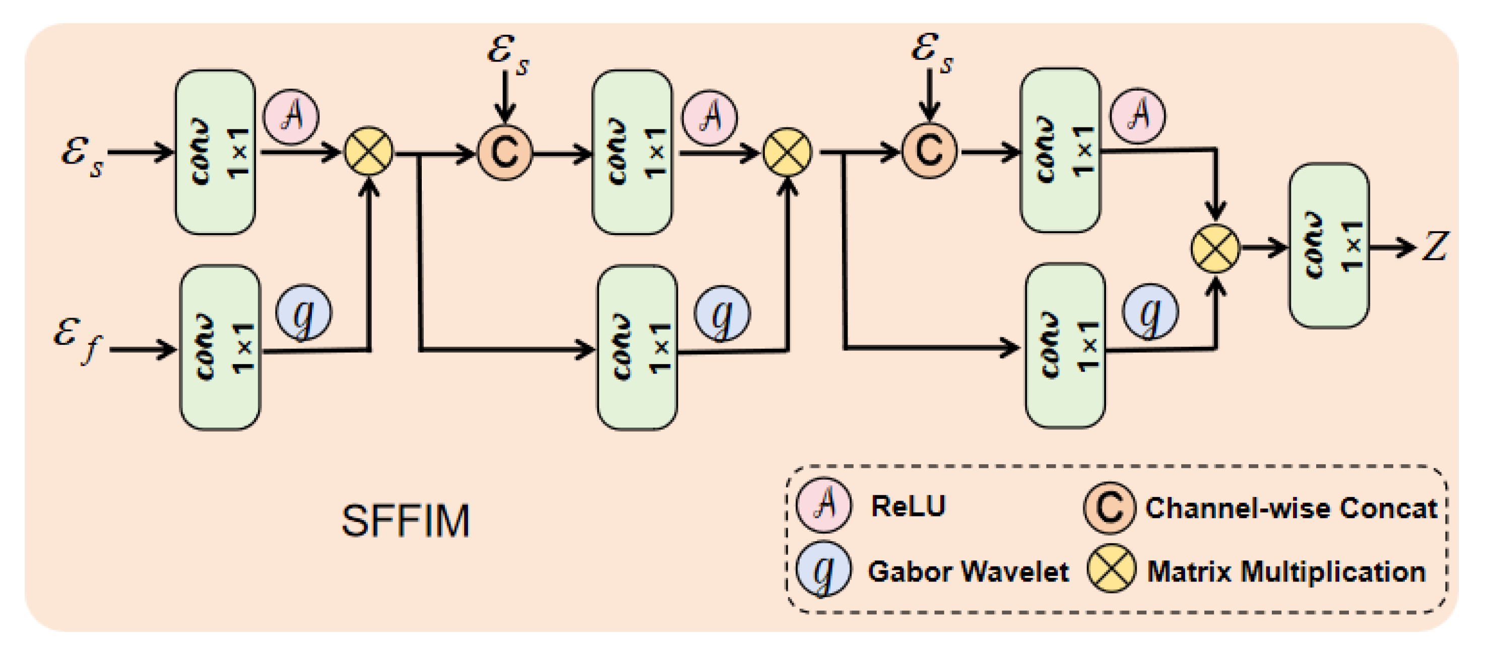
The Spatial–Frequency Feature Interaction Module (SFFIM) is designed to seamlessly fuse the spatial feature map and frequency-domain feature map obtained from the FSFIFM module. Specifically, the Spatial–Frequency Interactive Decoder (SFID) consists of three layers, taking spatial features and frequency-domain features as inputs. Its outputs I HR and I HR r - up jointly contribute to the generation of the final fused image ( I ˜ R H × W × D ). The feature interaction process is illustrated in Figure 2. The complex Gabor wavelet function is defined as follows:
G w ( x ^ ) = e j a x e | b x ^ | 2 .
where a denotes the center frequency in the frequency domain, b is a constant (which can be regarded as the standard deviation of the Gaussian function), and x ^ is a vector in the time domain (or spatial domain). In this paper, a and b are learnable parameters, and the settings of their initial values are shown in Table 1.

4. Experiment

4.1. Datasets and Implementation Details

To assess the performance of FIMamba, we carried out experiments on three datasets featuring different spatial and spectral resolutions, allowing for a thorough evaluation of the fusion capabilities across varying data distributions. The datasets include 8-band imagery from the WorldView-3 (WV3) sensor (DigitalGlobe, Westminster, CO, USA), and 4-band imagery from QuickBird (QB) sensor (DigitalGlobe, Westminster, CO, USA) and GaoFen-2 (GF2) sensor (China Aerospace Science and Technology Corporation, Beijing, China).
Each dataset contains image triplets composed of a Panchromatic (PAN) image, a Low-Resolution Multispectral (LRMS) image, and a Ground Truth (GT) image, with dimensions of 64 × 64 , 16 × 16 × 8 , and 64 × 64 × 8 , respectively. The datasets and preprocessing procedures follow those provided in the PanCollection repository [45].
During training, we implement our network using the PyTorch 3.8 framework on an RTX 4070D GPU. The learning rate is set to 1 × 10 4 and we employ the l 1 loss function along with the Adam optimizer [46], using a batch size of 4. Specifically, for the training set, we set the input sample size to 64 × 64 and the total number of epochs to 1000.
Different evaluation metrics are employed for test sets depending on their respective resolutions. Specifically, we employ SAM [47], ERGAS [48], and Q8 [49] to assess the performance of FIMamba on the reduced resolution datasets, and D s , D λ , and HQNR [50] to evaluate its performance on the full-resolution datasets.

4.2. Results

4.2.1. Results on the WorldView-3 Dataset

The performance of FIMamba was assessed using 20 test images from the WorldView-3 (WV3) dataset. Results under both reduced-resolution and full-resolution conditions are summarized in Table 2.
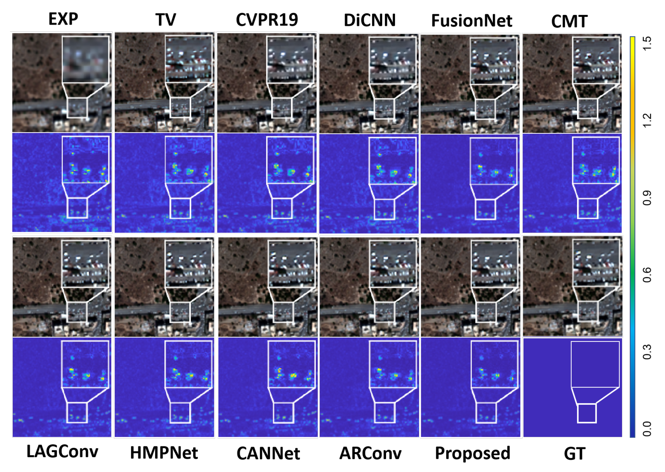
FIMamba was compared with three conventional pansharpening methods as well as several state-of-the-art deep learning approaches. To visually demonstrate the differences in performance, fusion results and corresponding error maps for selected methods are shown in Figure 3, with key regions highlighted in enlarged views for detailed examination.
Quantitative evaluation on the reduced-resolution dataset indicates that FIMamba achieves state-of-the-art performance. In particular, it reaches a SAM value of 2.835 and an ERGAS value of 2.128, outperforming all competing deep learning methods. The error maps further reveal that images produced by FIMamba are more consistent with the ground truth (GT) images.
Additionally, to assess the model’s performance on real-world full-resolution data, this study utilizes three no-reference evaluation metrics: spectral distortion ( D λ ), spatial distortion ( D s ), and hybrid quality with no reference (HQNR). Table 2 reports the average performance of the selected public dataset across full-resolution (FR) samples. The findings indicate that the FFIMamba model not only maintains the optimal average performance but also exhibits the smallest standard deviation—clear evidence of its superiority and enhanced stability. As illustrated in Figure 3, visual results from the full-resolution WV3 dataset further show that the output of the proposed method retains richer detail and delivers superior visual quality.
In the full-resolution image generation task on the WV3 dataset, the proposed FIMamba method achieves state-of-the-art performance. The HQNR metric is used to evaluate the quality of full-resolution image fusion, and its value is close to 1, indicating that the generated high-resolution multispectral images (HRMSI) retain excellent quality, as shown in Figure 4. These results demonstrate that FIMamba can effectively integrate HRMSI data while minimizing spatial and spectral distortions, verifying its strong generalization ability in full-resolution scenarios.

4.2.2. Results on QuickBird (QB)

In this section, the performance of the proposed FIMamba method is assessed on the QuickBird (QB) dataset. Table 3 summarizes the performance metrics of both traditional and deep learning-based methods. The results indicate that FIMamba achieves the best overall performance. However, regarding the Q4 metric, its performance is slightly lower than that of ARConv. This discrepancy may be attributed to limitations in spectral consistency and detail preservation, suggesting potential areas for further improvement in the proposed method.

4.2.3. Results on GaoFen-2 (GF2)

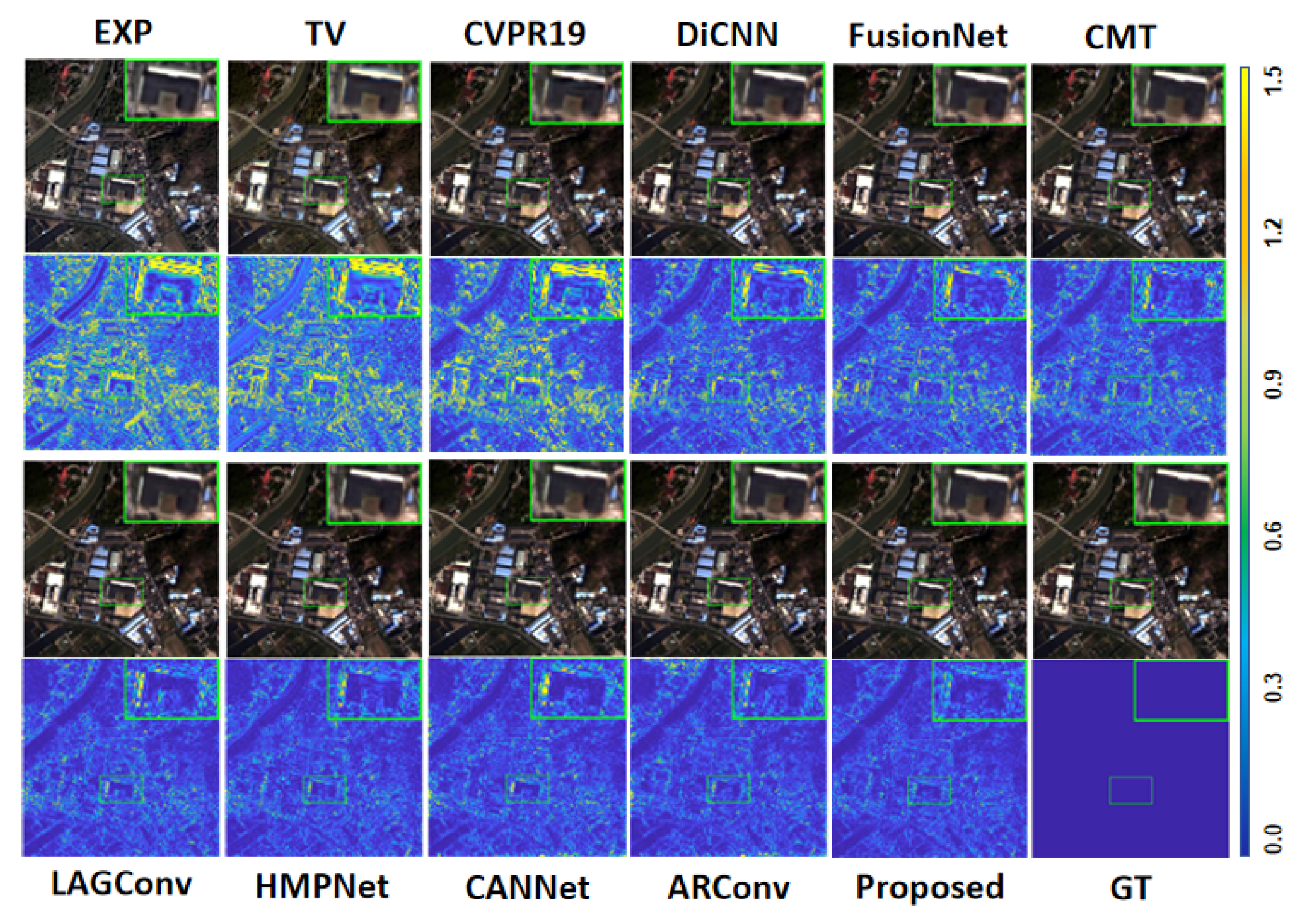
On the reduced-resolution dataset of GaoFen-2 (GF2), we tested the proposed method using 20 test images, and the results are shown in Table 4. The proposed method also achieves state-of-the-art (SOTA) performance on this dataset. From the error maps in Figure 5, it can be observed that there are still significant performance differences between traditional fusion methods and deep learning-based fusion methods.

4.2.4. Results on the WorldView2 Dataset

To assess the generalization capability of the FFIMamba model, we carried out additional experimental validation on the publicly available WorldView-2 (WV2) dataset. Since experiments had already been completed on three other datasets, we limited the comparisons to the proposed model and classical pansharpening algorithms. The corresponding results are summarized in Table 5. It can be seen from the data in this table that FFIMamba achieves superior performance over the other methods across all evaluation metrics, which confirms the model’s strong generalization ability.

4.3. Ablation Studies

To assess how individual components influence the performance of the FIMamba network, we carried out ablation tests on the WV3 and GF2 datasets. These tests involved systematically excluding key modules one by one, with four specific experimental setups: (a) without the VSSM module, (b) without the SARSSM module, (c) without the FSFIFM module, and (d) without the SFFIM module. Quantitative results from these experiments are presented in Table 6 and Table 7, serving as a foundation for evaluating the role of each component. An analysis of the data in Table 6 and Table 7 reveals a consistent trend: removing any single component leads to a noticeable drop in FIMamba’s overall performance. This finding confirms that every module plays a necessary role in the network’s architecture and that no component can be easily replaced or removed without compromising functionality. Notably, the most substantial performance declines occur in the test groups where the VSSM module (group a) and SARSSM module (group b) are excluded. This observation underscores the critical value of integrating Visual Mamba into the FIMamba framework—its inclusion directly contributes to the network’s ability to capture essential features and maintain high fusion accuracy in pansharpening tasks.

4.3.1. Significance of VSSM

The VSSM module serves as a central component for extracting deep global features. In the ablation experiment where this module was removed (results in Table 6 and Table 7), the performance metrics dropped noticeably, emphasizing the crucial role of VSSM in capturing global contextual information. These findings indicate that VSSM is an essential element for FIMamba to achieve high-quality outputs.

4.3.2. Core Value of the SARSSM

The SARSSM module plays a vital role in deep feature extraction. In the ablation study, the SARSSM module was removed, and the fusion was performed using only the SFEM, FSFIFM, and SFFIM modules. As reported in Table 6 and Table 7, the performance metrics decreased, highlighting the importance of the Mamba-based SARSSM module in generating high-quality feature representations at the network’s front end, thereby improving the network’s capacity to extract effective features.

4.3.3. Importance of FSFIFM

The FSFIFM module is essential for capturing high-frequency details in FIMamba, playing a significant role in feature enhancement and fusion. To assess its contribution, FSFIFM was removed from the model and replaced with a conventional implicit neural representation. As presented in Table 6 and Table 7, this modification led to a noticeable decline in image quality, demonstrating that FSFIFM is crucial for extracting richer high-frequency features.

4.3.4. Indispensability of SFFIM

In high-dimensional multimodal feature fusion, traditional approaches often rely on simple feature addition or concatenation, which may neglect the varying contributions of different feature dimensions. The SFFIM module in FIMamba enables interactive feature fusion to address this limitation. In the ablation study, SFFIM was replaced with a standard feature addition operation, and the output channels were adjusted via subsequent convolutional layers to satisfy the dimensional requirements of hyperspectral images (HSI). As reported in Table 6 and Table 7, this substitution caused a noticeable drop in model performance. These results demonstrate that the SFFIM module more effectively balances and integrates information across multi-source features, enhancing fusion capability and improving overall feature fusion quality.

4.3.5. Comparison of Upsampling Methods

Implicit Neural Representations (INRs) are often treated as interpolation tools, offering additional information and parameterized weight generation within the spatial domain. In this work, we evaluate the performance of INR-based upsampling in comparison with other commonly used upsampling methods. Specifically, the INR module was replaced with the pixel-shuffle technique [64] as well as standard bilinear and bicubic interpolation methods. As shown in Table 8, the INR-based upsampling consistently outperforms these alternatives in the pansharpening task, highlighting the effectiveness and advantages of our proposed interpolation approach.

4.3.6. Inference Time

Inference time is one of the important metrics for evaluating the efficiency of pansharpening methods. In Table 9, we compare the inference time of FIMamba with that of ARConv, DCFNet, MMNet, and LAGConv. Tests on these methods and our proposed method (FIMamba) at a resolution of 256 × 256 show that our method only takes 0.383 s to fuse high-resolution multispectral (HRMS) images. While this inference time is longer than that of ARConv and MMNet, it may be attributed to the higher computational complexity of our model. Currently, we are focusing on developing a more lightweight framework.

5. Limitation

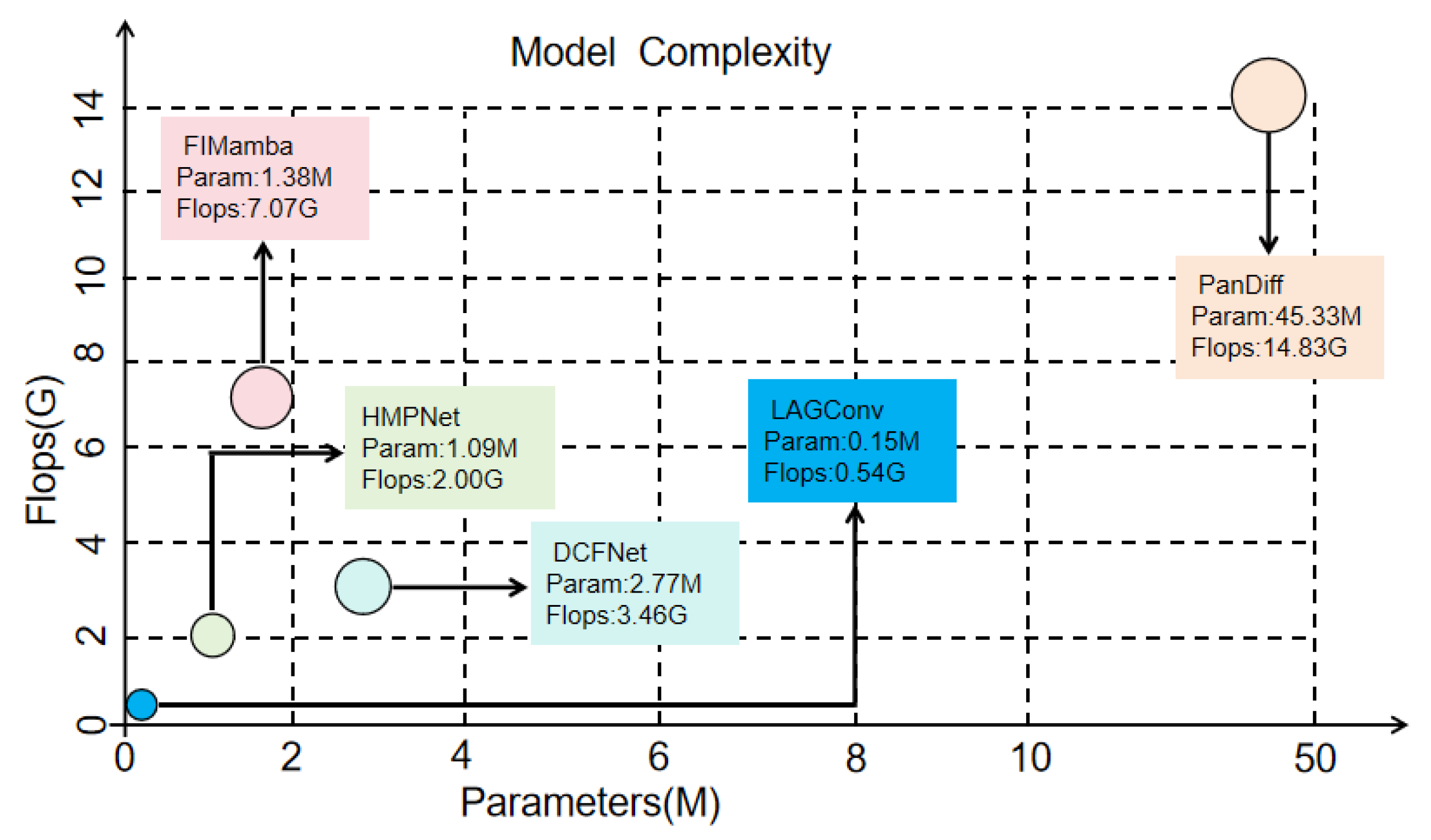
While the FFIMamba approach developed in this study delivers strong results for remote sensing image pansharpening, three key limitations remain to be addressed. First, computational efficiency is a bottleneck. The method incurs a computational load of 7.07 G FLOPs; even though its parameter count (1.38 M) is moderate, its inference time for 256 × 256 resolution images reaches 0.383 s—longer than that of comparison methods like ARConv (0.336 s) and MMNet (0.348 s). This high computational complexity poses challenges for deploying the model on resource-limited devices or portable platforms, which are common in real-world remote sensing applications. Second, performance in specific evaluation metrics still has room for refinement. On the Q4 metric (a key indicator of spectral–spatial fusion quality) for the QuickBird (QB) dataset, FFIMamba achieves a score of 0.936 ± 0.041, slightly underperforming ARConv’s 0.939 ± 0.081. This gap is likely tied to constraints in the method’s strategies for maintaining spectral consistency and preserving fine details, preventing it from gaining a clear edge in this critical metric. Third, the model lacks sufficient lightweight design. When compared to lightweight pansharpening methods such as LAGConv—which operates with just 0.15 M parameters and 2.00 G FLOPs—FFIMamba’s architectural choices (including multi-module coordination and Fourier domain feature processing) enhance fusion accuracy but also drive up model complexity. As a result, the method has not yet struck an optimal balance between high accuracy and lightweight deployment, limiting its adaptability to scenarios where hardware resources are constrained.

6. Discussion

The comprehensive experimental results indicate that FIMamba is a pansharpening approach that combines high accuracy with strong generalization capabilities. The model demonstrates consistent performance across three diverse datasets, including 4-band imagery from GaoFen-2 (GF2) and QuickBird (QB), as well as 8-band data from WorldView-3 (WV3), which features more complex spectral information. These results suggest that the FIMamba architecture is not restricted to specific data types and effectively addresses the inherent challenges of pansharpening tasks. In particular, on the WV3 dataset, key spectral metrics such as ERGAS, SAM, and Q8 exceed those of existing methods, confirming the effectiveness of the proposed network in comprehensively modeling and processing both spatial and spectral information from multispectral and panchromatic images.
Nevertheless, some limitations remain. As shown in Figure 6, which compares the complexity of different models, FIMamba requires approximately 1.38 M parameters and 7.07 G FLOPs. While the parameter count is moderate, the computational cost remains relatively high. Therefore, developing a more lightweight network represents an important avenue for future research, which is currently under active exploration. Additionally, in terms of the Q4 metric on the QB dataset, the difference between the proposed method and ARConv is relatively small. This may be due to certain similarities in the texture detail preservation strategies of the two methods; future work will further optimize the feature interaction mechanism to expand the advantage in this metric.

7. Conclusions

This study introduces a novel pansharpening approach that effectively combines local and global features, offering significant advantages in capturing high-frequency details. By exploiting the Mamba architecture for long-range dependency modeling and utilizing Fourier-based implicit neural representations to process features continuously in the spatial–frequency domain, the proposed FIMamba framework achieves superior reconstruction of spatial and spectral information. Experimental results on multiple datasets demonstrate the robustness and effectiveness of the method, emphasizing its potential to enhance remote sensing applications. Future research will aim to further improve fusion quality and optimize computational efficiency, facilitating deployment on resource-limited and portable platforms.

Author Contributions

Conceptualization, Z.-Z.H.; data curation, Y.-J.L.; investigation, Z.-Z.H. and Y.-J.L.; methodology, Z.-Z.H. and Y.-J.L.; resources, H.-X.D.; software, Z.-Z.H.; visualization, Z.-Z.H.; writing—original draft, Z.-Z.H.; writing—review and editing, Y.-J.L. and H.-X.D. All authors have read and agreed to the published version of the manuscript.

Funding

This work is supported by the Natural Science Foundation of Sichuan Province (Grant No. 2023NSFSC1341).

Data Availability Statement

The link to the dataset used in this article is as follows: https://liangjiandeng.github.io/PanCollection.html (accessed on 5 September 2025).

Acknowledgments

During the preparation of this manuscript, the authors used ChatGPT-4.0 for text polishing. The authors have reviewed and edited the output generated by this tool and take full responsibility for the entire content of this publication. We are grateful to the editors and reviewers for their advice.

Conflicts of Interest

The authors declare no conflicts of interest.

References

  1. Sishodia, R.P.; Ray, R.L.; Singh, S.K. Applications of Remote Sensing in Precision Agriculture: A Review. Remote Sens. 2020, 12, 3136. [Google Scholar] [CrossRef]
  2. Wang, J.; Miao, J.; Li, G.; Tan, Y.; Yu, S.; Liu, X.; Zeng, L.; Li, G. Pan-Sharpening Network of Multi-Spectral Remote Sensing Images Using Two-Stream Attention Feature Extractor and Multi-Detail Injection (TAMINet). Remote Sens. 2023, 16, 75. [Google Scholar] [CrossRef]
  3. Wang, Z.G.; Kang, Q.; Xun, Y.J.; Shen, Z.Q.; Cui, C.B. Military reconnaissance application of high-resolution optical satellite remote sensing. In Proceedings of the International Symposium on Optoelectronic Technology and Application 2014: Optical Remote Sensing Technology and Applications, Beijing, China, 13–15 May 2014; Volume 9299, pp. 301–305. [Google Scholar]
  4. Wei, X.; Yuan, M. Adversarial pan-sharpening attacks for object detection in remote sensing. Pattern Recognit. 2023, 139, 109466. [Google Scholar] [CrossRef]
  5. Rokni, K. Investigating the impact of Pan Sharpening on the accuracy of land cover mapping in Landsat OLI imagery. Geod. Cartogr. 2023, 49, 12–18. [Google Scholar] [CrossRef]
  6. Bovolo, F.; Bruzzone, L.; Capobianco, L.; Garzelli, A.; Marchesi, S.; Nencini, F. Change detection from pansharpened images: A comparative analysis. IEEE Geosci. Remote Sens. Lett. 2010, 7, 53–57. [Google Scholar] [CrossRef]
  7. Feng, X.; Wang, J.; Zhang, Z.; Chang, X. Remote sensing image pan-sharpening via Pixel difference enhance. Int. J. Appl. Earth Obs. Geoinf. 2024, 132, 104045. [Google Scholar] [CrossRef]
  8. Choi, J.; Yu, K.; Kim, Y. A New Adaptive Component-Substitution-Based Satellite Image Fusion by Using Partial Replacement. IEEE Trans. Geosci. Remote Sens. 2011, 49, 295–309. [Google Scholar] [CrossRef]
  9. Vivone, G. Robust Band-Dependent Spatial-Detail Approaches for Panchromatic Sharpening. IEEE Trans. Geosci. Remote Sens. 2019, 57, 6421–6433. [Google Scholar] [CrossRef]
  10. Vivone, G.; Restaino, R.; Chanussot, J. Full Scale Regression-Based Injection Coefficients for Panchromatic Sharpening. IEEE Trans. Image Process. 2018, 27, 3418–3431. [Google Scholar] [CrossRef]
  11. Vivone, G.; Restaino, R.; Dalla Mura, M.; Licciardi, G.; Chanussot, J. Contrast and Error-Based Fusion Schemes for Multispectral Image Pansharpening. IEEE Geosci. Remote Sens. Lett. 2014, 11, 930–934. [Google Scholar] [CrossRef]
  12. Fu, X.; Lin, Z.; Huang, Y.; Ding, X. A Variational Pan-Sharpening with Local Gradient Constraints. In Proceedings of the 2019 IEEE/CVF Conference on Computer Vision and Pattern Recognition (CVPR), Long Beach, CA, USA, 15–20 June 2019; pp. 10257–10266. [Google Scholar] [CrossRef]
  13. Tian, X.; Chen, Y.; Yang, C.; Ma, J. Variational Pansharpening by Exploiting Cartoon-Texture Similarities. IEEE Trans. Geosci. Remote Sens. 2022, 60, 1–16. [Google Scholar] [CrossRef]
  14. Wang, D.; Li, Y.; Ma, L.; Bai, Z.; Chan, J.C.W. Going Deeper with Densely Connected Convolutional Neural Networks for Multispectral Pansharpening. Remote Sens. 2019, 11, 2608. [Google Scholar] [CrossRef]
  15. Wang, Z.; Wu, S.; Xie, W.; Chen, M.; Prisacariu, V.A. NeRF–: Neural Radiance Fields Without Known Camera Parameters. arXiv 2022, arXiv:2102.07064. [Google Scholar] [CrossRef]
  16. Lv, J.; Guo, J.; Zhang, Y.; Zhao, X.; Lei, B. Neural Radiance Fields for High-Resolution Remote Sensing Novel View Synthesis. Remote Sens. 2023, 15, 3920. [Google Scholar] [CrossRef]
  17. Lee, J.; Jin, K.H. Local Texture Estimator for Implicit Representation Function. arXiv 2022, arXiv:2111.08918. [Google Scholar] [CrossRef]
  18. Chen, Y.; Liu, S.; Wang, X. Learning Continuous Image Representation with Local Implicit Image Function. arXiv 2021, arXiv:2012.09161. [Google Scholar] [CrossRef]
  19. Chen, H.W.; Xu, Y.S.; Hong, M.F.; Tsai, Y.M.; Kuo, H.K.; Lee, C.Y. Cascaded Local Implicit Transformer for Arbitrary-Scale Super-Resolution. arXiv 2023, arXiv:2303.16513. [Google Scholar] [CrossRef]
  20. Sitzmann, V.; Martel, J.N.P.; Bergman, A.W.; Lindell, D.B.; Wetzstein, G. Implicit Neural Representations with Periodic Activation Functions. arXiv 2020, arXiv:2006.09661. [Google Scholar] [CrossRef]
  21. Rahaman, N.; Baratin, A.; Arpit, D.; Draxler, F.; Lin, M.; Hamprecht, F.A.; Bengio, Y.; Courville, A. On the Spectral Bias of Neural Networks. arXiv 2019, arXiv:1806.08734. [Google Scholar] [CrossRef]
  22. Gilles, J.; Tran, G.; Osher, S. 2D Empirical Transforms. Wavelets, Ridgelets, and Curvelets Revisited. SIAM J. Imaging Sci. 2014, 7, 157–186. [Google Scholar] [CrossRef]
  23. Loui, A.; Venetsanopoulos, A.; Smith, K. Morphological autocorrelation transform: A new representation and classification scheme for two-dimensional images. IEEE Trans. Image Process. 1992, 1, 337–354. [Google Scholar] [CrossRef]
  24. Grigoryan, A. Method of paired transforms for reconstruction of images from projections: Discrete model. IEEE Trans. Image Process. 2003, 12, 985–994. [Google Scholar] [CrossRef]
  25. Xu, X.; Wang, Z.; Shi, H. UltraSR: Spatial Encoding is a Missing Key for Implicit Image Function-based Arbitrary-Scale Super-Resolution. arXiv 2022, arXiv:2103.12716. [Google Scholar] [CrossRef]
  26. Nguyen, Q.H.; Beksi, W.J. Single Image Super-Resolution via a Dual Interactive Implicit Neural Network. arXiv 2022, arXiv:2210.12593. [Google Scholar] [CrossRef]
  27. Tang, J.; Chen, X.; Zeng, G. Joint Implicit Image Function for Guided Depth Super-Resolution. In Proceedings of the 29th ACM International Conference on Multimedia, MM ’21, Virtual, 20–24 October 2021; pp. 4390–4399. [Google Scholar] [CrossRef]
  28. Dian, R.; Li, S.; Fang, L. Learning a Low Tensor-Train Rank Representation for Hyperspectral Image Super-Resolution. IEEE Trans. Neural Netw. Learn. Syst. 2019, 30, 2672–2683. [Google Scholar] [CrossRef]
  29. Yang, Y.; Xing, Z.; Yu, L.; Huang, C.; Fu, H.; Zhu, L. Vivim: A Video Vision Mamba for Medical Video Segmentation. arXiv 2024, arXiv:2401.14168. [Google Scholar] [CrossRef]
  30. Yang, Y.; Wu, L.; Huang, S.; Wan, W.; Tu, W.; Lu, H. Multiband Remote Sensing Image Pansharpening Based on Dual-Injection Model. IEEE J. Sel. Top. Appl. Earth Obs. Remote Sens. 2020, 13, 1888–1904. [Google Scholar] [CrossRef]
  31. Zhao, C.; Cai, W.; Dong, C.; Hu, C. Wavelet-based Fourier Information Interaction with Frequency Diffusion Adjustment for Underwater Image Restoration. arXiv 2023, arXiv:2311.16845. [Google Scholar] [CrossRef]
  32. Chi, L.; Jiang, B.; Mu, Y. Fast fourier convolution. In Proceedings of the 34th International Conference on Neural Information Processing Systems, NIPS ’20, Vancouver, BC, Canada, 6–12 December 2020. [Google Scholar]
  33. Rao, Y.; Zhao, W.; Zhu, Z.; Lu, J.; Zhou, J. Global Filter Networks for Image Classification. arXiv 2021, arXiv:2107.00645. [Google Scholar] [CrossRef]
  34. Li, C.; Guo, C.L.; Zhou, M.; Liang, Z.; Zhou, S.; Feng, R.; Loy, C.C. Embedding Fourier for Ultra-High-Definition Low-Light Image Enhancement. arXiv 2023, arXiv:2302.11831. [Google Scholar] [CrossRef]
  35. Gu, A.; Goel, K.; Ré, C. Efficiently Modeling Long Sequences with Structured State Spaces. arXiv 2022, arXiv:2111.00396. [Google Scholar] [CrossRef]
  36. Xie, X.; Cui, Y.; Tan, T.; Zheng, X.; Yu, Z. FusionMamba: Dynamic Feature Enhancement for Multimodal Image Fusion with Mamba. arXiv 2025, arXiv:2404.09498. [Google Scholar] [CrossRef]
  37. Guo, H.; Li, J.; Dai, T.; Ouyang, Z.; Ren, X.; Xia, S.T. MambaIR: A Simple Baseline for Image Restoration with State-Space Model. arXiv 2024, arXiv:2402.15648. [Google Scholar] [CrossRef]
  38. Zhang, Q.; Zhang, X.; Quan, C.; Zhao, T.; Huo, W.; Huang, Y. Mamba-STFM: A Mamba-Based Spatiotemporal Fusion Method for Remote Sensing Images. Remote Sens. 2025, 17, 2135. [Google Scholar] [CrossRef]
  39. Zhu, Q.; Cai, Y.; Fang, Y.; Yang, Y.; Chen, C.; Fan, L.; Nguyen, A. Samba: Semantic Segmentation of Remotely Sensed Images with State Space Model. arXiv 2024, arXiv:2404.01705. [Google Scholar] [CrossRef]
  40. Yan, L.; Feng, Q.; Wang, J.; Cao, J.; Feng, X.; Tang, X. A Multilevel Multimodal Hybrid Mamba-Large Strip Convolution Network for Remote Sensing Semantic Segmentation. Remote Sens. 2025, 17, 2696. [Google Scholar] [CrossRef]
  41. Chen, K.; Chen, B.; Liu, C.; Li, W.; Zou, Z.; Shi, Z. RSMamba: Remote Sensing Image Classification with State Space Model. IEEE Geosci. Remote Sens. Lett. 2024, 21, 1–5. [Google Scholar] [CrossRef]
  42. Liao, J.; Wang, L. HyperspectralMamba: A Novel State Space Model Architecture for Hyperspectral Image Classification. Remote Sens. 2025, 17, 2577. [Google Scholar] [CrossRef]
  43. Press, W.H.; Teukolsky, S.A.; Vetterling, W.T.; Flannery, B.P. Numerical Recipes 3rd Edition: The Art of Scientific Computing, 3rd ed.; Cambridge University Press: New York, NY, USA, 2007. [Google Scholar]
  44. Keys, R. Cubic convolution interpolation for digital image processing. IEEE Trans. Acoust. Speech Signal Process. 1981, 29, 1153–1160. [Google Scholar] [CrossRef]
  45. Deng, L.j.; Vivone, G.; Paoletti, M.E.; Scarpa, G.; He, J.; Zhang, Y.; Chanussot, J.; Plaza, A. Machine Learning in Pansharpening: A benchmark, from shallow to deep networks. IEEE Geosci. Remote Sens. Mag. 2022, 10, 279–315. [Google Scholar] [CrossRef]
  46. Kingma, D.P.; Ba, J. Adam: A Method for Stochastic Optimization. arXiv 2017, arXiv:1412.6980. [Google Scholar] [CrossRef]
  47. Boardman, J.W. Automating Spectral Unmixing of AVIRIS Data Using Convex Geometry Concepts. 1993. Available online: https://ntrs.nasa.gov/citations/19950017428 (accessed on 10 November 2025).
  48. Wald, L. Data Fusion. Definitions and Architectures—Fusion of Images of Different Spatial Resolutions; École des Mines Paris—PSL: Paris, France, 2002. [Google Scholar]
  49. Garzelli, A.; Nencini, F. Hypercomplex Quality Assessment of Multi/Hyperspectral Images. IEEE Geosci. Remote Sens. Lett. 2009, 6, 662–665. [Google Scholar] [CrossRef]
  50. Arienzo, A.; Vivone, G.; Garzelli, A.; Alparone, L.; Chanussot, J. Full-Resolution Quality Assessment of Pansharpening: Theoretical and hands-on approaches. IEEE Geosci. Remote Sens. Mag. 2022, 10, 168–201. [Google Scholar] [CrossRef]
  51. Aiazzi, B.; Alparone, L.; Baronti, S.; Garzelli, A. Context-driven fusion of high spatial and spectral resolution images based on oversampled multiresolution analysis. IEEE Trans. Geosci. Remote Sens. 2002, 40, 2300–2312. [Google Scholar] [CrossRef]
  52. Palsson, F.; Sveinsson, J.R.; Ulfarsson, M.O. A New Pansharpening Algorithm Based on Total Variation. IEEE Geosci. Remote Sens. Lett. 2014, 11, 318–322. [Google Scholar] [CrossRef]
  53. Wu, Z.C.; Huang, T.Z.; Deng, L.J.; Huang, J.; Chanussot, J.; Vivone, G. LRTCFPan: Low-Rank Tensor Completion Based Framework for Pansharpening. IEEE Trans. Image Process. 2023, 32, 1640–1655. [Google Scholar] [CrossRef]
  54. Masi, G.; Cozzolino, D.; Verdoliva, L.; Scarpa, G. Pansharpening by Convolutional Neural Networks. Remote Sens. 2016, 8, 594. [Google Scholar] [CrossRef]
  55. Yang, J.; Fu, X.; Hu, Y.; Huang, Y.; Ding, X.; Paisley, J. PanNet: A Deep Network Architecture for Pan-Sharpening. In Proceedings of the 2017 IEEE International Conference on Computer Vision (ICCV), Venice, Italy, 22–29 October 2017; pp. 1753–1761. [Google Scholar] [CrossRef]
  56. He, L.; Rao, Y.; Li, J.; Chanussot, J.; Plaza, A.; Zhu, J.; Li, B. Pansharpening via Detail Injection Based Convolutional Neural Networks. IEEE J. Sel. Top. Appl. Earth Obs. Remote Sens. 2019, 12, 1188–1204. [Google Scholar] [CrossRef]
  57. Deng, L.J.; Vivone, G.; Jin, C.; Chanussot, J. Detail Injection-Based Deep Convolutional Neural Networks for Pansharpening. IEEE Trans. Geosci. Remote Sens. 2021, 59, 6995–7010. [Google Scholar] [CrossRef]
  58. Wu, X.; Huang, T.Z.; Deng, L.J.; Zhang, T.J. Dynamic Cross Feature Fusion for Remote Sensing Pansharpening. In Proceedings of the 2021 IEEE/CVF International Conference on Computer Vision (ICCV), Montreal, QC, Canada, 10–17 October 2021; pp. 14667–14676. [Google Scholar] [CrossRef]
  59. Jin, Z.R.; Zhang, T.J.; Jiang, T.X.; Vivone, G.; Deng, L.J. LAGConv: Local-Context Adaptive Convolution Kernels with Global Harmonic Bias for Pansharpening. Proc. AAAI Conf. Artif. Intell. 2022, 36, 1113–1121. [Google Scholar] [CrossRef]
  60. Tian, X.; Li, K.; Zhang, W.; Wang, Z.; Ma, J. Interpretable Model-Driven Deep Network for Hyperspectral, Multispectral, and Panchromatic Image Fusion. IEEE Trans. Neural Netw. Learn. Syst. 2024, 35, 14382–14395. [Google Scholar] [CrossRef]
  61. Shu, W.J.; Dou, H.X.; Wen, R.; Wu, X.; Deng, L.J. CMT: Cross Modulation Transformer with Hybrid Loss for Pansharpening. IEEE Geosci. Remote Sens. Lett. 2024, 21, 1–5. [Google Scholar] [CrossRef]
  62. Duan, Y.; Wu, X.; Deng, H.; Deng, L.J. Content-Adaptive Non-Local Convolution for Remote Sensing Pansharpening. In Proceedings of the 2024 IEEE/CVF Conference on Computer Vision and Pattern Recognition (CVPR), Seattle, WA, USA, 16–22 June 2024; pp. 27738–27747. [Google Scholar] [CrossRef]
  63. Wang, X.; Zheng, Z.; Shao, J.; Duan, Y.; Deng, L.J. Adaptive Rectangular Convolution for Remote Sensing Pansharpening. arXiv 2025, arXiv:2503.00467. [Google Scholar] [CrossRef]
  64. Shi, W.; Caballero, J.; Huszár, F.; Totz, J.; Aitken, A.P.; Bishop, R.; Rueckert, D.; Wang, Z. Real-Time Single Image and Video Super-Resolution Using an Efficient Sub-Pixel Convolutional Neural Network. In Proceedings of the 2016 IEEE Conference on Computer Vision and Pattern Recognition (CVPR), Las Vegas, NV, USA, 27–30 June 2016; pp. 1874–1883. [Google Scholar] [CrossRef]
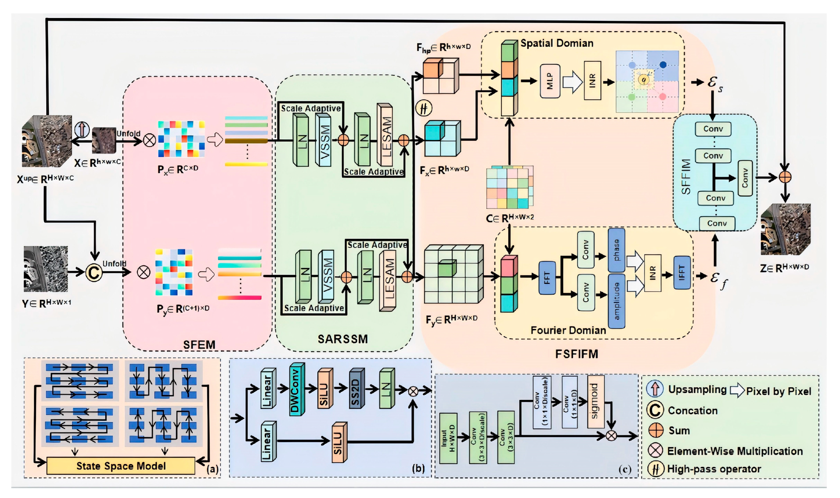
Figure 1. The flowchart of the Fourier Fusion Implicit Mamba Network (FFIMamba) framework. (a) SS2D. (b) VisionSSM. (c) LESAM.
Remotesensing 17 03747 g001
Figure 2. Detailed composition of the proposed Spatial–Frequency Feature Interaction Module (SFFIM).
Remotesensing 17 03747 g002
Figure 3. Qualitative Result Comparison of Representative Methods on the WV3 Reduced-Resolution Dataset. The RGB images output by each model are presented in the first and third rows, while the residual maps when compared with the ground truth images are shown in the second and fourth rows.
Remotesensing 17 03747 g003
Figure 4. Visual comparisons involving some representative pansharpening methods on one example of the full resolution WV3 dataset. True-color fused images are depicted in the first row. The second row is devoted to the HQNR maps.
Remotesensing 17 03747 g004
Figure 5. Qualitative Result Comparison of Representative Methods on the GF2 Reduced-Resolution Dataset. The RGB images output by each model are presented in the first and third rows, while the residual maps when compared with the ground truth images are shown in the second and fourth rows.
Remotesensing 17 03747 g005
Figure 6. Complexity statistics.
Remotesensing 17 03747 g006
Table 1. Hyperparameter Summary of the FFIMamba Model.
Hyperparameter CategorySpecific ParameterParameter ValueDescription
Network Structure ParametersSliding Window Size (k) 3 × 3 Applied in the Shallow Feature Extraction Module (SFEM) for local feature aggregation. It scans the image to unfold regional information via a sliding window; the value is determined by empirical tuning.
Feature Channel Number (D)64Used to define the dimension of the projection matrix in SFEM, which maps input features to a unified latent feature space; the value is determined by empirical tuning.
Channel Compression Ratio (r) 1 / 4 Utilized for channel compression in the 3D convolution of the Local Enhanced Spectral Attention Module (LESAM). It reduces computational cost and enhances spectral representation; the value is determined by empirical tuning.
Frequency Encoding Hyperparameter (m)10Employed for frequency encoding of relative position coordinates in the spatial implicit fusion function, controlling the encoding dimension; the value is determined by empirical tuning.
Gabor Wavelet Param. (a) for SFFIM30 (initial value)Controls the center frequency of the Gabor wavelet in the frequency domain (a learnable parameter); the initial value is determined by empirical tuning.
Gabor Wavelet Param. (b) for SFFIM10 (initial value)Controls the standard deviation of the Gaussian function in the Gabor wavelet (a learnable parameter); the initial value is determined by empirical tuning.
Training ParametersLearning Rate 1 × 10 4 Set for the Adam optimizer to control the parameter update step size; the value is determined by empirical tuning.
Batch Size4Number of samples input in each training iteration; the value is determined by empirical tuning.
Training Epochs1000Total number of complete training cycles of the model on the training set; the value is determined by empirical tuning.
Input Sample Size 64 × 64 Size of image samples input to the model during training; the value is determined by empirical tuning.
Loss Function L 1 LossUsed to calculate the error between the model’s predictions and the ground truth (GT), guiding parameter optimization; the selection is determined by empirical tuning.
OptimizerAdamOptimization algorithm for model parameter updates; the selection is determined by empirical tuning.
Table 2. Performance benchmarking on the WV3 dataset was conducted using 20 reduced-resolution and 20 full-resolution samples. The top-performing results are highlighted in bold, while the second-best are indicated with an underline.
MethodsReduced-Resolution MetricsFull-Resolution Metrics
SAM ↓ERGAS ↓ Q8 ↑ D λ D s HQNR ↑
EXP [51] 5.800 ± 1.881 7.155 ± 1.878 0.627 ± 0.092 0.023 ± 0.007 0.0813 ± 0.032 0.897 ± 0.036
TV [52] 5.692 ± 1.808 4.856 ± 1.434 0.795 ± 0.120 0.023 ± 0.006 0.039 ± 0.023 0.938 ± 0.027
MTF-GLP-FS [10] 5.316 ± 1.766 4.700 ± 1.597 0.833 ± 0.092 0.020 ± 0.008 0.063 ± 0.029 0.919 ± 0.035
BSDS-PC [9] 5.429 ± 1.823 4.698 ± 1.617 0.829 ± 0.097 0.063 ± 0.024 0.073 ± 0.036 0.870 ± 0.053
CVPR2019 [12] 5.207 ± 1.574 5.484 ± 1.505 0.764 ± 0.088 0.030 ± 0.006 0.041 ± 0.014 0.931 ± 0.018
LRTCFPan [53] 4.737 ± 1.412 4.315 ± 1.442 0.846 ± 0.091 0.018 ± 0.007 0.0528 ± 0.026 0.931 ± 0.031
PNN [54] 3.680 ± 0.763 2.682 ± 0.648 0.893 ± 0.092 0.021 ± 0.008 0.043 ± 0.015 0.937 ± 0.021
PanNet [55] 3.616 ± 0.766 2.666 ± 0.689 0.891 ± 0.093 0.017 ± 0.007 0.047 ± 0.021 0.937 ± 0.027
DiCNN [56] 3.593 ± 0.762 2.673 ± 0.663 0.900 ± 0.087 0.036 ± 0.011 0.046 ± 0.0175 0.920 ± 0.026
FusionNet [57] 3.325 ± 0.698 2.467 ± 0.645 0.904 ± 0.090 0.024 ± 0.009 0.036 ± 0.014 0.941 ± 0.020
DCFNet [58] 3.038 ± 0.585 2.165 ± 0.499 0.913 ± 0.087 0.019 ± 0.007 0.034 ± 0.005 0.948 ± 0.012
LAGConv [59] 3.104 ± 0.559 2.300 ± 0.613 0.910 ± 0.091 0.037 ± 0.015 0.042 ± 0.015 0.923 ± 0.025
HMPNet [60] 3.063 ± 0.577 2.229 ± 0.545 0.916 ± 0.087 0.018 ± 0.007 0.053 ± 0.053 0.930 ± 0.011
CMT [61] 2.994 ± 0.607 2.214 ± 0.516 0.917 ± 0.085 0.021 ± 0.008 0.037 ± 0.008 0.943 ± 0.014
CANNet [62] 2.930 ± 0.593 2.158 ± 0.515 0.920 ± 0.084 0.020 ± 0.008 0.030 ± 0.007 0.951 ± 0.013
ARConv [63] 2.885 ± 0.590 ̲ 2.139 ± 0.528 ̲ 0.921 ± 0.083 ̲ 0.015 ± 0.006 ̲ 0.028 ± 0.007 ̲ 0.958 ± 0.010 ̲
Proposed 2 . 835 ± 0 . 513 2 . 128 ± 0 . 452 0 . 929 ± 0 . 094 0 . 014 ± 0 . 005 0 . 027 ± 0 . 006 0 . 960 ± 0 . 032
Table 3. Performance benchmarking on the QB dataset using 20 reduced-resolution samples. Best in bold; second best underlined.
MethodsSAM ↓ERGAS ↓Q4 ↑
EXP [51] 8.435 ± 1.925 11.819 ± 1.905 0.584 ± 0.075
TV [52] 7.565 ± 1.535 7.781 ± 0.699 0.820 ± 0.090
MTF-GLP-FS [10] 7.093 ± 1.816 7.374 ± 0.724 0.835 ± 0.080
BSD-PC [9] 8.898 ± 1.980 7.515 ± 0.800 0.831 ± 0.098
CVPR2019 [12] 7.988 ± 1.820 6.959 ± 1.268 0.737 ± 0.087
LRTCFPan [53] 7.197 ± 1.711 9.328 ± 0.812 0.855 ± 0.087
PNN [54] 5.205 ± 0.963 4.472 ± 0.373 0.918 ± 0.094
PanNet [55] 5.791 ± 1.184 5.863 ± 0.888 0.885 ± 0.092
DiCNN [56] 5.380 ± 1.027 5.135 ± 0.481 0.904 ± 0.090
FusionNet [57] 4.923 ± 0.908 4.159 ± 0.328 0.925 ± 0.094
DCFNet [58] 4.512 ± 0.773 3.809 ± 0.336 0.934 ± 0.087
LAGConv [59] 4.547 ± 0.830 3.826 ± 0.420 0.934 ± 0.088
HMPNet [60] 4.617 ± 0.404 3.404 ± 0.478 ̲ 0.936 ± 0.102
CMT [61] 4.535 ± 0.822 3.744 ± 0.321 0.935 ± 0.086
CANNet [62] 4.507 ± 0.835 3.652 ± 0.327 0.937 ± 0.083 ̲
ARConv [63] 4.430 ± 0.811 ̲ 3.633 ± 0.327 0 . 939 ± 0 . 081
Proposed 4 . 411 ± 0 . 511 3 . 395 ± 0 . 127 0.936 ± 0.041
Table 4. Performance benchmarking on the GF2 dataset using 20 reduced-resolution samples. Best in bold; second best underlined.
MethodsSAM ↓ERGAS ↓Q4 ↑
EXP [51] 1.820 ± 0.403 2.366 ± 0.554 0.812 ± 0.051
TV [52] 1.918 ± 0.398 1.745 ± 0.405 0.905 ± 0.027
MTF-GLP-FS [10] 1.655 ± 0.385 1.589 ± 0.395 0.897 ± 0.035
BSD-PC [9] 1.681 ± 0.360 1.667 ± 0.445 0.892 ± 0.035
CVPR2019 [12] 1.598 ± 0.353 1.877 ± 0.448 0.886 ± 0.028
LRTCFPan [53] 1.315 ± 0.283 1.301 ± 0.313 0.932 ± 0.033
PNN [54] 1.048 ± 0.226 1.057 ± 0.236 0.960 ± 0.010
PanNet [55] 0.997 ± 0.212 0.919 ± 0.191 0.967 ± 0.010
DiCNN [56] 1.053 ± 0.231 1.081 ± 0.254 0.959 ± 0.010
FusionNet [57] 0.974 ± 0.212 0.988 ± 0.222 0.964 ± 0.009
DCFNet [58] 0.872 ± 0.169 0.784 ± 0.146 0.974 ± 0.009
LAGConv [59] 0.786 ± 0.148 0.687 ± 0.113 0.981 ± 0.008
HMPNet [60] 0.803 ± 0.141 0 . 564 ± 0 . 099 0.981 ± 0.020
CMT [61] 0.753 ± 0.138 0.648 ± 0.109 0.982 ± 0.007
CANNet [62] 0.707 ± 0.148 0.630 ± 0.128 0.983 ± 0.006 ̲
ARConv [63] 0.698 ± 0.149 ̲ 0.626 ± 0.127 0.983 ± 0.007
Proposed 0 . 687 ± 0 . 158 0.574 ± 0.134 ̲ 0 . 984 ± 0 . 005
Table 5. Quantitative Results on WV2 Dataset for Pansharpening. Best in bold.
MethodsSAM ↓ERGAS ↓SCC ↑Q2n ↑
EXP [51] 5.230 ± 1.245 6.872 ± 1.563 0.785 ± 0.081 0.821 ± 0.076
TV [52] 4.915 ± 1.192 5.638 ± 1.427 0.802 ± 0.075 0.843 ± 0.069
MTF-GLP-FS [10] 4.562 ± 1.084 5.124 ± 1.316 0.823 ± 0.068 0.865 ± 0.062
BDS-PC [9] 4.328 ± 1.057 4.987 ± 1.254 0.837 ± 0.063 0.879 ± 0.058
PNN [54] 3.548 ± 0.892 3.956 ± 1.032 0.876 ± 0.052 0.918 ± 0.045
PanNet [55] 3.317 ± 0.854 3.624 ± 0.987 0.889 ± 0.048 0.930 ± 0.041
DiCNN [56] 3.185 ± 0.826 3.472 ± 0.953 0.897 ± 0.045 0.938 ± 0.038
FusionNet [57] 3.024 ± 0.793 3.258 ± 0.921 0.905 ± 0.042 0.946 ± 0.035
Proposed 2 . 786 ± 0 . 731 2 . 745 ± 0 . 849 0 . 928 ± 0 . 034 0 . 965 ± 0 . 028
Table 6. Quantitative Evaluation of Ablation Studies on GF2 datasets. Best in bold. w/o means ‘without’.
MethodsSAM ↓ERGAS ↓Q8 ↑
(a) w/o VSSM 0.702 ± 0.303 0.604 ± 0.355 0.934 ± 0.043
(b) w/o SARSSM 0.709 ± 0.154 0.611 ± 0.242 0.943 ± 0.051
(c) w/o FSFIFM 0.698 ± 0.114 0.587 ± 0.162 0.975 ± 0.045
(d) w/o SFFIM 0.695 ± 0.248 0.592 ± 0.142 0.967 ± 0.065
Proposed 0 . 687 ± 0 . 158 0 . 574 ± 0 . 134 0 . 984 ± 0 . 005
Table 7. Quantitative Evaluation of Ablation Studies on WV3 datasets. Best in bold. w/o means ‘without’.
MethodsSAM ↓ERGAS ↓Q8 ↑
(a) w/o VSSM 2.979 ± 0.603 2.262 ± 0.455 0.921 ± 0.083
(b) w/o SARSSM 3.021 ± 0.254 2.369 ± 0.142 0.912 ± 0.061
(c) w/o FSFIFM 2.875 ± 0.314 2.159 ± 0.562 0.915 ± 0.085
(d) w/o SFFIM 2.865 ± 0.368 2.146 ± 0.342 0.923 ± 0.035
Proposed 2 . 835 ± 0 . 513 2 . 128 ± 0 . 452 0 . 929 ± 0 . 094
Table 8. Quantitative comparisons with other upsampling methods on the WV3 dataset.
MethodsSAM (↓)ERGAS (↓)Q8 (↑)
Bilinear 2.921 ± 0.625 2.165 ± 0.521 0.918 ± 0.083
Bicubic 2.915 ± 0.364 2.147 ± 0.612 0.919 ± 0.079
Pixel Shuffle 2.890 ± 0.471 2.159 ± 0.511 0.923 ± 0.034
Proposed 2 . 835 ± 0 . 513 2 . 128 ± 0 . 452 0 . 929 ± 0 . 094
Table 9. Efficiency results on the 256 × 256 WV3 reduced-resolution datasets.
MethodFIMmambaARConvDCFNetMMNetLAGConv
Runtime (s)0.3830.3360.5480.3481.381
Disclaimer/Publisher’s Note: The statements, opinions and data contained in all publications are solely those of the individual author(s) and contributor(s) and not of MDPI and/or the editor(s). MDPI and/or the editor(s) disclaim responsibility for any injury to people or property resulting from any ideas, methods, instructions or products referred to in the content.