MSFFNet: Multimodal Spatial–Frequency Fusion Network for RGB-DSM Remote Sensing Image Segmentation

Highlights

What are the main findings?

• The integration of wavelet transform in multimodal feature fusion significantly enhances the model’s ability to preserve edge information.
• The fusion strategy enables early interaction of complementary information and effectively improves feature discriminability through feature enhancement.

What is the implication of the main finding?

• The study provides a solution to improve edge clarity in remote sensing image segmentation.
• The study provides a key solution to enhance segmentation capability under multimodal fusion.

Abstract

Remote sensing image segmentation is essential for resource planning and disaster monitoring. Although RGB-based methods are widely adopted, they often exhibit suboptimal performance in distinguishing objects with similar color and texture characteristics. The fusion of height information from Digital Surface Models (DSM) aids in the discrimination of these challenging objects. However, existing CNN- and pooling-based fusion methods tend to lose edge details as network depth increases, resulting in blurred segmentation boundaries. To address this issue, a Multimodal Spatial–Frequency Fusion Network (MSFFNet) is proposed to effectively enhance edge details by fusing high-level frequency and spatial features. Specifically, a Hybrid Branch Fusion Module (HBFM) is proposed, in which the wavelet transform branch decomposes features into sub-components, effectively isolating edge and structural information from other textures. Such a process in the frequency domain prevents edge details from being lost or diluted during fusion, thereby preserving boundary clarity in segmentation. Additionally, a Multi-Scale Contextual Attention Module (MSCAM) is proposed to capture multi-scale contextual information for enhancing spatial feature representation, while adjusting both spatial and channel-wise attention mechanisms to improve detail and accuracy. Experiments over benchmark Vaihingen and Potsdam datasets demonstrate that the proposed approach can clearly enhance edge delineation while improving segmentation accuracy.

1. Introduction

Remote sensing image segmentation is a vital task in the interpretation of remote sensing data and holds significant value in various domains, including land use planning, urban development [1,2], disaster monitoring [3,4], resource exploration, military surveillance, and ecological monitoring [5,6]. Semantic segmentation, in particular, involves classifying each pixel in an image into a specific land cover category, enabling a comprehensive understanding of the landscape [7,8,9,10,11,12,13,14]. Advancing research in semantic segmentation of remote sensing images and achieving accurate object delineation are essential for promoting the development and application of remote sensing technology.

The fine-grained and multi-scale characteristics of remote sensing images pose significant obstacles to improving the accuracy of single-modality semantic segmentation. To address the inherent limitations of single-modality information, researchers have increasingly adopted multimodal approaches. For instance, RGB images capture visual color information, while Digital Surface Models (DSM) provide height data for ground objects. Due to differences in imaging mechanisms, modality heterogeneity, and suboptimal fusion strategies, multimodal fusion may suffer from insufficient feature complementarity and the loss of crucial information, ultimately leading to reduced segmentation accuracy. Moreover, visually similar objects in RGB imagery are difficult to distinguish, increasing the likelihood of misclassification. In such cases, incorporating height information from DSM can effectively differentiate objects and enhance segmentation accuracy. As shown in Figure 1, although buildings and impervious surfaces exhibit similar visual characteristics in the RGB image, their height differences are clearly distinguishable in the DSM image, which helps to reduce segmentation confusion. This highlights the advantage of DSM in capturing edge information, which contributes to more accurate object and boundary recognition.

In recent years, several multimodal remote sensing segmentation methods have adopted dual-branch architectures to capture and fuse RGB and DSM features, achieving promising segmentation performance [15,16,17,18,19,20,21,22,23,24,25]. As network depth increases, these fusion strategies often suffer from issues such as the loss of edge information and blurred object boundaries. Blurred boundaries can obscure the distinction between different targets, potentially causing the model to misclassify two entirely different objects as the same class or as unrelated classes. Moreover, partial overlap and mixing between target regions may occur, disrupting the original feature distribution. This negatively impacts both feature extraction and fusion, ultimately leading to a decline in segmentation accuracy. Such issues are critical and should not be overlooked in multimodal fusion tasks.

As a classic frequency-domain technique, wavelet transform has been widely applied in multimodal image processing. It decomposes features into low- and high-frequency components, where the low-frequency components capture global contextual information, and the high-frequency components preserve edge details. For instance, BSANet [26] employs wavelet transform for upsampling and downsampling in its dual-branch design. DWU-Net [27] and XNet [28] decompose images into high- and low-frequency components and apply separate U-Nets for each. HaarFuse [29] extracts features from optical and infrared images using wavelet convolution and fuses them via wavelet decomposition. WaveCRNet [30] introduces wavelet priors via a wavelet attention module embedded in its PID network, and reconstructs features using dual-tree complex wavelet transforms. WaveFusion [31] combines wavelet transform and self-attention to enhance fused features, while HaarNet [32] applies wavelet decomposition to RGB and depth features before convolutional fusion. These approaches collectively reflect the growing trend of integrating frequency-domain analysis with dual-branch architectures, which has become a prevailing framework for improved multimodal representation. Our work follows this direction but introduces a novel design for deeper-level feature fusion and enhancement, aiming to preserve more complete modality-specific information and improve overall fusion effectiveness.

To address issues such as boundary blurring and the loss of edge information during fusion, we introduce wavelet transform and propose a multimodal remote sensing segmentation network that integrates RGB and DSM data, aiming to further enhance segmentation accuracy [33,34]. Specifically, we design a hybrid branch fusion module, where RGB features are processed through a convolutional branch and DSM features are processed through a wavelet-based branch, effectively combining information from both the convolutional and frequency domains. In addition, we introduce a spatial-channel attention module to strengthen the model’s capacity for multi-scale contextual modeling, thereby improving feature representation and segmentation performance.

Although numerous studies [26,27,28,29,30,31,32,35,36,37] have explored the integration of wavelet transform into dual-branch architectures to improve multimodal image fusion and segmentation performance, most existing methods typically either treat wavelet transform as a preprocessing or auxiliary operation during the early encoding stages, or impose a tightly coupled fusion strategy that directly integrates features from different modalities. However, these designs often lack deeper-level fusion and enhancement mechanisms. As network depth increases, such limitations may lead to redundant or diluted representations across modalities and hinder the preservation of critical feature information.

Unlike previous methods, our approach introduces several significant differences. First, we adopt a decoupled design that maintains independent encoding paths for RGB and DSM in both the external dual-branch encoders and the internal hybrid fusion module. The proposed framework performs progressive fusion and enhancement of features from each encoder level. The fused features are not fed back into the original encoder paths but are passed through a decoder with progressive upsampling to produce the final segmentation map. This architecture not only preserves modality-specific representations by decoupling multimodal fusion from single-modality feature extraction, but also facilitates effective cross-modal feature interaction, while avoiding the redundancy and mutual interference that can arise from feeding fused features back into the encoder paths.

Second, unlike previous methods that apply wavelet transforms uniformly to all modalities, we selectively integrate the wavelet attention module into the DSM branch within the fusion module. Since DSM features are less rich than RGB features, applying wavelet transforms to both RGB and DSM can degrade feature quality and obscure the distinct information inherent to each modality, ultimately reducing segmentation accuracy. Therefore, we apply the wavelet transform specifically to the DSM branch to extract both high-frequency edge information and low-frequency structural information, leveraging the DSM modality’s advantage in providing clear boundary delineation. The RGB branch, in contrast, retains a convolutional structure to better capture its strengths in texture and structural feature extraction. Furthermore, unlike other methods, our wavelet attention module introduces wavelet transforms into the Transformer [38] architecture. Combined with a gating mechanism, it not only captures long-range dependencies but also filters salient DSM features and controls the flow of effective information.

In summary, our design differs from existing approaches in terms of fusion strategy, branch decoupling, and the selective application of wavelet transform. Without compromising modality independence, it enhances boundary modeling capability and improves segmentation accuracy. The main contributions of this work are summarized as follows:

1.

To retain more edge information during the fusion process, a Multimodal Spatial–Frequency Fusion Network (MSFFNet) is constructed, which fuses edge features in the wavelet domain and spatial features in the convolutional domain, thereby enhancing edge representation as well as improving segmentation accuracy.

2.

To highlight edge information in the frequency domain, a Hybrid Branch Fusion Module (HBFM) is constructed, which decomposes DSM features into multiple sub-components by wavelet transform, from which high-frequency edge features are separately extracted and processed. Such process in the frequency domain prevents mixing with irrelevant features and alleviates edge information loss during the fusion process.

3.

To enhance spatial contextual information, a Multi-Scale Contextual Attention Module (MSCAM) is constructed, which aggregates multi-scale spatial information and applies self-attention to refine channel-wise features, improving intra-class consistency while effectively distinguishing inter-class differences.

The rest of this paper is structured as follows: Section 2 reviews related works, Section 3 details the proposed method, Section 4 presents experimental evaluations to validate its effectiveness, and Section 6 summarizes the conclusions.

2. Related Works

2.1. Single-Modal Semantic Segmentation

With the rapid development of deep learning, numerous semantic segmentation methods originally proposed in computer vision, such as FCN [39], UNet [40], PSPNet [41], SegNet [42], DeepLabv3+ [43], and SegFormer [44], have been widely adapted to remote sensing tasks. Recent approaches like DPFANet [45] adopt dual-encoder structures combining Transformer and CNN with adaptive fusion strategies. MAResUNet [46] enhances UNet with attention mechanisms, while LSKNet [47] introduces a lightweight design with dynamic receptive fields for remote sensing scenarios. LANet [48] and AerialFormer [49] focus on hierarchical feature fusion and Transformer-based multi-scale representation, respectively. Other efforts, such as Swin-based methods [50] and ResUNet-a [51], integrate Transformer backbones or multi-task modules to further improve contextual understanding and segmentation performance.

RS3Mamba [52] introduces Mamba-based layer normalization to overcome limitations of CNNs and Transformers. MCAT-UNet [53] enhances UNet with a cross-shaped Transformer and multi-scale convolution to reduce computational cost and improve edge segmentation. Dual-domain Transformer [54] incorporates FFT and edge attention into Swin Transformer for better edge feature capture. CGGLNet [55] employs multi-level fusion via self-attention to enhance contextual understanding. CRFNet [56] integrates CRF-based potential learning into the segmentation pipeline. Edge-aware designs, such as those by Chen et al. [57], LSRFormer [58], and UNetFormer [59], further refine segmentation by focusing on fine-grained details through Transformer-based U-shaped networks. HRNet [60] employs the concept of hierarchical relation learning to explore the correspondence between query and support samples. It extracts features from both the query and support images, and then processes them through multi-level relational processors to obtain relational representations. Unlike our proposed method, HRNet focuses on a single modality and builds relational dependencies using convolutional and deformable transformer structures. In contrast, our approach first extracts information from different modalities through convolutional and wavelet branches, and then fuses the complementary features via a deep convolutional network.

2.2. Multimodal Semantic Segmentation

ASMFNet [15] introduced a segmentation network capable of fusing multimodal information across neighboring scales. FDGSNet [16] leveraged frequency decomposition to develop a gated segmentation network. TransFusion [61] integrated 2D images with 3D point clouds for enhanced segmentation. MFNet [62] combined high-resolution remote sensing imagery with LiDAR data to improve segmentation performance. PACSCNet [17] introduced a progressive adjacent-layer coordination symmetric cascade network to mitigate detail loss during multimodal fusion. MANet [18] incorporated the Segment Anything Model with multimodal adapters for enhanced segmentation. CaFE [19] integrated class prior knowledge and imbalanced learning techniques to refine segmentation accuracy. CMFNet [20], built on the Transformer architecture, employed a cross-attention mechanism to effectively fuse multimodal information.

MFTransNet [21] combines CNNs and Transformers for lightweight segmentation with balanced accuracy and efficiency. FTransUNet [22] leverages global average pooling to fuse shallow features. HAFNet [23] performs fusion at both shallow and output layers using RGB, DSM, and fusion branches. Du et al. [63] integrate SAR and optical images using Mamba [64] and diffusion models. AMIANet [65] fuses point clouds and images through an interactive fusion module. Zhang et al. [24] enhance dual-path fusion with spatial and channel attention. EndNet [66] and FusAtNet [67] fuse hyperspectral and LiDAR data, employing attention mechanisms to enrich spectral and spatial semantics.

IKD-Net [68] introduces an imbalance-aware fusion strategy where strong modalities guide weak ones via multi-stage deep fusion. Gao et al. [69] use GCNs to model pixel relationships from hyperspectral and LiDAR features. MFT [70] applies cross-attention between hyperspectral features and LiDAR-derived tokens in a Transformer framework. Hong et al. [71] adopt GANs to fuse hyperspectral and multispectral data. NCGLF2 [72] integrates local and global features from hyperspectral and LiDAR inputs. Audebert [25] improves SegNet with multi-kernel convolutions for multi-source fusion. ACNet [73] introduces a three-branch structure with channel attention for high-quality fusion. FuseNet [74] and ESANet [75] fuse RGB and depth data in unified segmentation architectures.

2.3. Wavelet-Based Image Segmentation and Fusion

Wavemix [33] utilizes wavelet transform for multi-scale modeling, while WaveSNet [76] adopts it for up/downsampling. WTNet [77] fuses RGB and depth features via wavelets. MISegNet [78] and SSW-AN [79] decompose images into wavelet sub-bands for encoding. WNet [80] embeds wavelets into a Transformer for denoising. DDFL [81] combines wavelets with pooling for dual-domain learning. WET-UNet [82] and Pan et al. [83] incorporate wavelet modules into UNet encoders to enhance structural feature extraction. Wave-ViT [84] integrates wavelets with self-attention for efficient downsampling and high accuracy. Liu et al. [35] introduced a dual-branch network, using wavelet-based high-frequency extraction and Transformer-based low-frequency modeling, followed by fusion and decoding. Hua et al. [36] employed a similar dual-encoder framework, integrating wavelet transform to decompose and fuse modality-specific features before decoding. FreqGAN [37] adopted a dual-branch design combining wavelet-based frequency decomposition with a hybrid fusion module and GAN-based training.

While these approaches are mostly rooted in medical imaging, their exploration in remote sensing remains limited. Our work adapts wavelet transform to multimodal remote sensing segmentation by integrating it into a Transformer-based architecture and proposing a hybrid branch fusion module for selective information guidance, mitigating modality-specific feature loss.

3. Method

3.1. Overall Framework

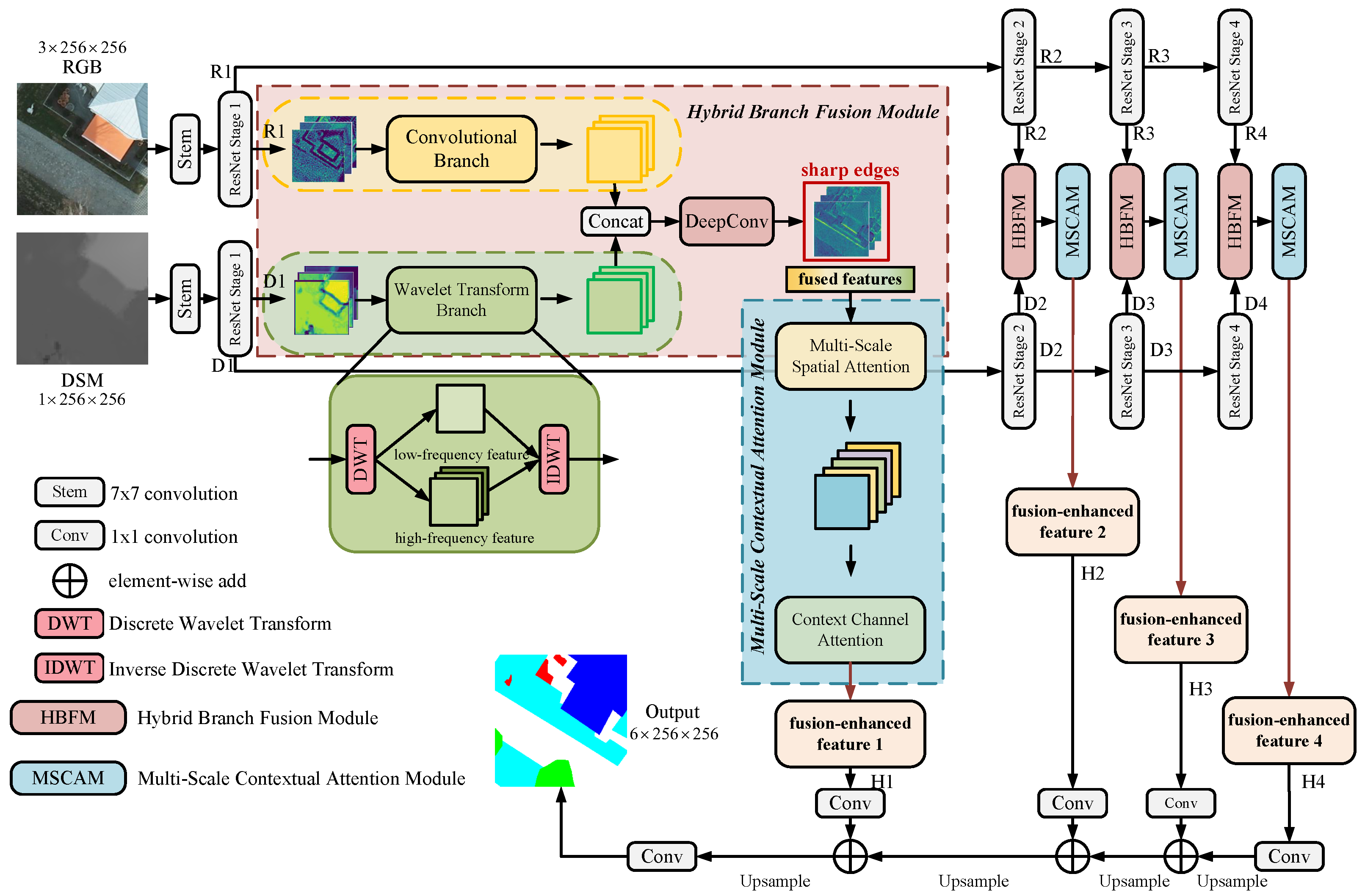
Multimodal remote sensing image segmentation requires an efficient fusion strategy. For two heterogeneous modalities, inappropriate fusion approaches can lead to information loss or redundancy. To address these issues, MSFFNet selectively extracts and fuses critical information from RGB and DSM in both spatial and frequency domains to enhance edge features, as illustrated in Figure 2.

The input to the network consists of RGB and DSM images. We use ResNet50 [85] as the encoder and Feature Pyramid Network (FPN) [86] as the decoder. The RGB image is processed through a ResNet-based encoder, generating four hierarchical feature maps denoted as P1, P2, P3, and P4. Similarly, the DSM data is passed through another ResNet encoder to produce four corresponding feature levels, D1, D2, D3, and D4. These two independent encoder branches enable each modality to fully extract its intrinsic features. Subsequently, the multi-level features from the RGB and DSM encoders are fused via the proposed HBFM and MSCAM modules, resulting in four fusion feature maps, H1, H2, H3, and H4. The fused features are then fed into a FPN, followed by conventional convolutional layers to generate the final segmentation map, as illustrated in Figure 2. It is noteworthy that the fused features are not fed back into the encoder branches. This decoupled design not only preserves the integrity of the modality-specific representations and avoids feature redundancy but also facilitates the complementary integration of heterogeneous information from different modalities. The following section provides a detailed explanation. The symbols used in this paper are summarized in

Table A1. Notation definitions used in this paper.

Symbol	Description
X, Y	Input features
$F_c$	Convolutional branch
$F_{wtm}$	Wavelet Transform Module (WTM) branch
$F_{pointc}$	$1\times 1$ pointwise convolution
$F_d$	Deep convolutional fusion network
$F_{HBFM}$	Output features of HBFM
$F_m$	MLP operation
$F_{gelu}$	GELU activation function
$F_{ln}$	Layer normalization
$F_{CB}$	Output features of the convolutional branch
$F_{WAM}$	Output features of the Wavelet Attention Module (WAM)
$F_{avgpools}$	Three average pooling layers
$F_{dwconvs}$	Four parallel large-kernel depthwise convolution layers
$X_M$	Output of the feed-forward neural network
$F_{CM}$	Output features of the Channel Mixer
$X_H$	Horizontally pooled features
$X_V$	Vertically pooled features
$X_{HV}$	Product of horizontally and vertically pooled features
$X_B$	Normalized result of $X_{HV}$
$X_{HV}^{\prime }$	Result of applying pointwise convolution and GELU to $X_B$
$X_{HV1}^{\prime }$	Result of applying a $5\times 5$ depthwise convolution to $X_{HV}^{\prime }$
$X_{HV}^{″}$	Summed result of multiple depthwise convolutions
$X_{MBC}$	Output features of the multi-branch convolution module
$X_{MSC}$	Output features of the multi-scale convolution module
$X_S$	Output features of the multi-scale spatial attention module
$X_D$	Result of applying average pooling and group normalization to $X_S$
$Q,K,V$	Features obtained by applying $1\times 1$ convolution to $X_D$
$X_{SA}$	Features after self-attention computation
$X_{MSCAM}$	Output features of the Multi-Scale Context Attention Module (MSCAM)
Concat	Channel-wise concatenation operation
$Con{v}_{i\times i}$	$i\times i$ convolution operation
$DWCon{v}_{i\times i}$	$i\times i$ depthwise convolution operation
$DWT$	Discrete Wavelet Transform
$IDWT$	Inverse Discrete Wavelet Transform
$LL,LH,HL,HH$	Four sub-band features after DWT
$\sigma$	Sigmoid activation function
$BatchNorm$	Batch normalization function
$GroupNorm$	Group normalization function
$TP,TN,FP,FN$	True Positives, True Negatives, False Positives, and False Negatives
$T{P}_c$, $T{N}_c$, $F{P}_c$, $F{N}_c$	Class-specific TP, TN, FP, and FN
$OA$	Overall Accuracy
$mIoU$	Mean Intersection over Union
$F1$	F1-score
$P_c$	Precision for class c
$R_c$	Recall for class c
$F{1}_c$	F1-score for class c

in the Appendix A.

3.2. Hybrid Branch Fusion Module

We propose a Hybrid Branch Fusion Module (HBFM), in which convolutional and wavelet branches independently process the RGB and DSM modalities. The resulting features are subsequently fused through a deep convolutional module, as illustrated in Figure 3.

RGB images typically contain richer structural, textural, and edge information, making convolutional processing particularly effective for capturing salient and diverse features. DSM images, by contrast, are single-channel grayscale representations with less spectral information but offer more precise boundary information—especially in scenarios where optical features are visually ambiguous. To exploit this complementarity, we utilize the frequency-domain capabilities of wavelet transform to further enhance edge features in DSM data. Accordingly, we assign the convolutional branch to process RGB features and the wavelet-based branch to handle DSM features. This design not only preserves the modality-specific representations but also facilitates the generation of more comprehensive and complementary fused features, thereby alleviating information loss during the fusion process.

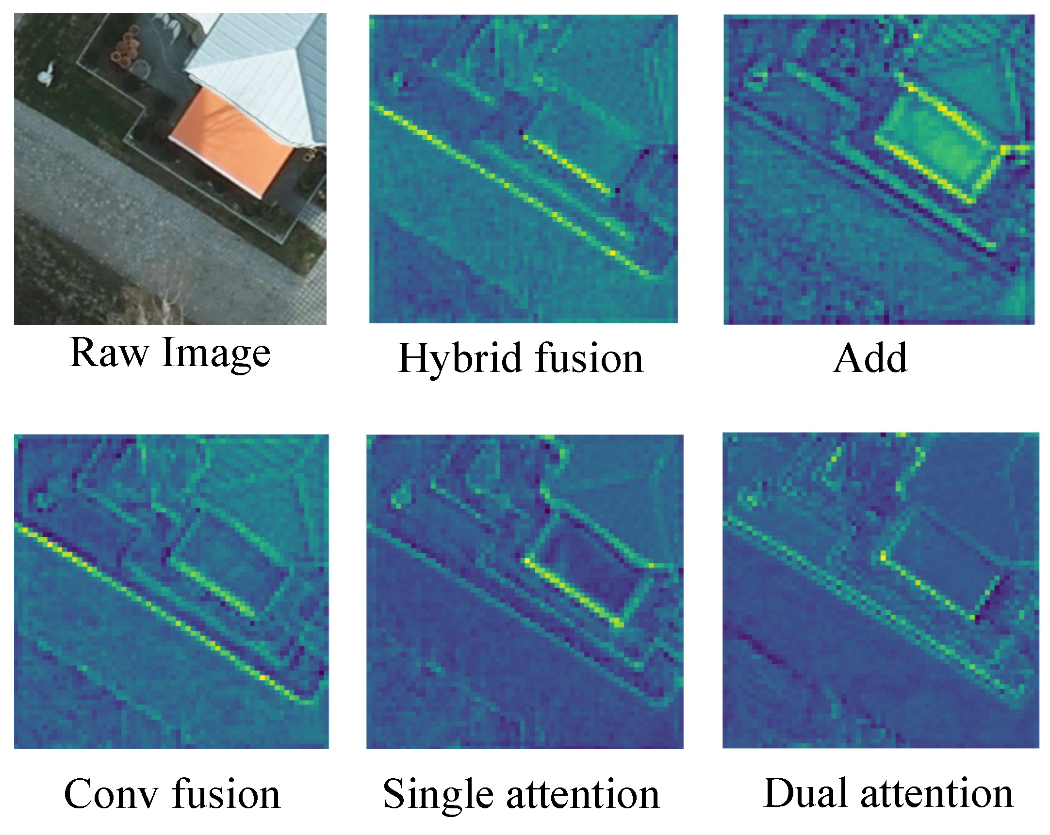
As shown in Figure 4, we compare our hybrid fusion method with several alternative fusion strategies by analyzing feature maps after the first encoder stage. The top row shows the input image, our hybrid fusion result, and addition-based fusion. The bottom row presents feature maps from convolution-only, spatial attention, channel attention, and dual-attention fusion. While all methods retain some edge details, our hybrid approach preserves clearer boundaries, particularly for impervious surfaces and low-lying vegetation. Moreover, when the boundaries between objects are blurred or indistinct, different targets may exhibit highly similar feature representations. As a result, the model is prone to misclassifying distinct objects as a single category, which adversely affects the segmentation performance. Through feature map comparisons, this highlights the module’s ability to retain modality-specific information and reduce feature loss during fusion. Additional quantitative results are provided in Section 4.

The input to HBFM consists of RGB features and DSM features, denoted as $X\in {\mathbb{R}}^{C\times H\times W}$ and $Y\in {\mathbb{R}}^{C\times H\times W}$, respectively, and is expressed as

$$F_{HBFM}=F_d\left(Concat(F_c\left(X\right),F_{wtm}\left(Y\right))\right)$$

(1)

$$F_{pointc}=Con{v}_{1\times 1}(·)$$

(2)

$$F_d=F_{pointc}\left(F_{pointc}\left(DWCon{v}_{1\times 1}\left(F_{pointc}(·)\right)\right)\right)$$

(3)

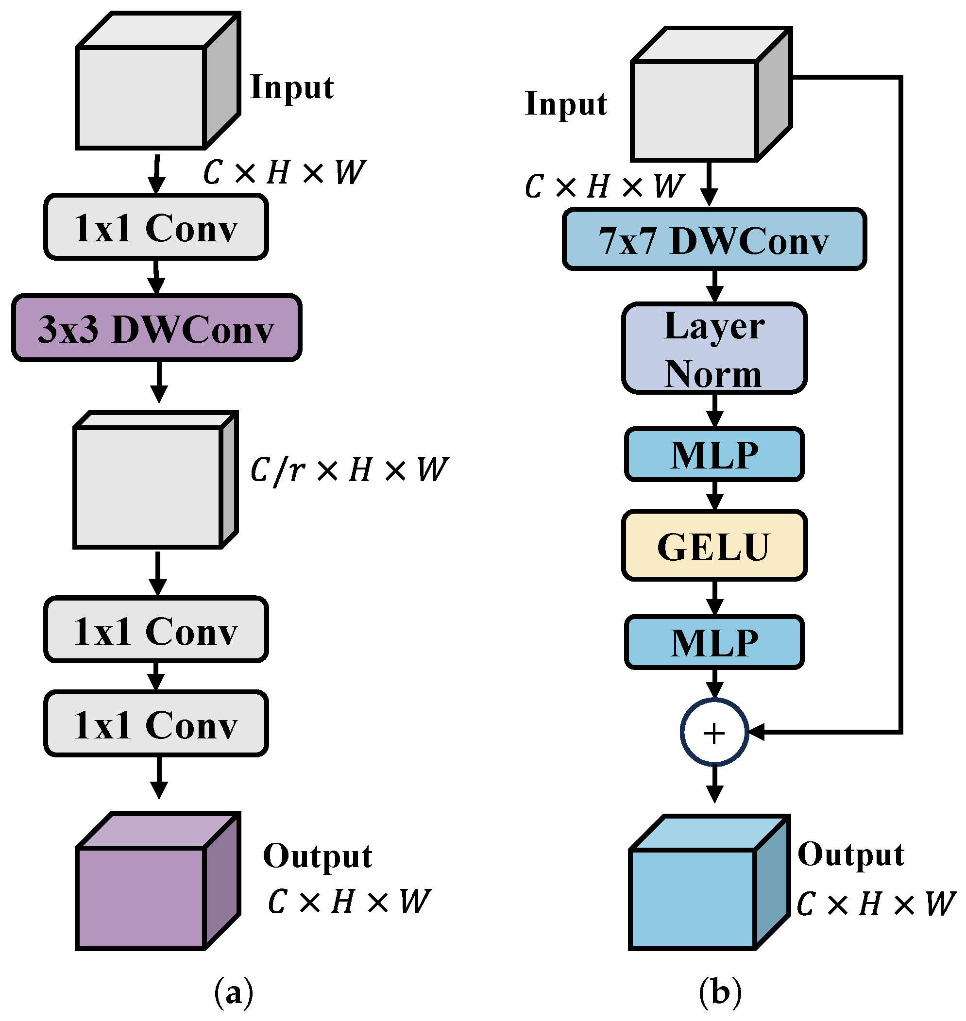
where $F_c$ represents the convolution branch composed of ConvNeXt blocks [87], and $F_{wtm}$ represents the wavelet transform branch. $Concat$ refers to the concatenation of inputs along the channel dimension. $F_d$ represents the depthwise convolution (Deep Conv) fusion network, whose detailed structure is illustrated in Figure 5.

$Con{v}_{1\times 1}$ represents the convolution module composed of $1\times 1$ convolution, GELU activation function, and batch normalization. Depending on the parameters of the convolution module, the configuration of the activation function and batch normalization may change. $DWCon{v}_{3\times 3}$ represents a $3\times 3$ depthwise convolution, where the number of groups equals the number of channels. In the hybrid branch module, the first point convolution after concatenation includes the activation function and batch normalization, with output channels of C. The depthwise convolution and the second point convolution also include activation functions and batch normalization. The last point convolution does not include an activation function but has batch normalization.

3.2.1. Convolution Branch

Although Transformer-based models have achieved impressive results in the field of semantic segmentation in recent years, and research on convolutional neural networks has decreased, we believe that the convolutional structure still has its irreplaceable advantages. Compared to Transformers, its inductive bias and local receptive field are key to capturing local features. We use ConvNeXt Blocks as the main components of the convolution branch, and the detailed structure is shown in Figure 5. The mathematical expression of the convolution branch is as follows:

$$F_m=MLP(·)$$

(4)

$$F_{CB}=F_m\left(F_{gelu}\left(F_m\left(F_{ln}\left(DWCon{v}_{7\times 7}\left(X\right)\right)\right)\right)\right)+X$$

(5)

where $X\in {\mathbb{R}}^{C\times H\times W}$ represents the RGB features input to the convolution branch. $DWCon{v}_{7\times 7}$ refers to depthwise convolutions, where the number of groups equals the number of channels, with a convolution kernel size of $7\times 7$. $F_{ln}$ represents layer normalization, $MLP$ stands for a multi-layer perceptron, and $F_{gelu}$ denotes the GELU activation function. $F_{CB}$ denotes the feature output of the convolutional branch. The convolution branch stacks three identical ConvNeXt Blocks in the third-level fusion module, while only one ConvNeXt Block is used in other fusion modules.

The convolution branch processes RGB features using a $7\times 7$ depthwise convolution followed by layer normalization. A feed-forward network with GELU activation then expands and reduces the feature dimensions. Residual connections are employed to preserve information. This branch integrates concepts from both convolutional networks and Transformers, employing an inverted bottleneck structure and large-kernel convolutions to expand the receptive field. By leveraging the local-detail capturing capability of convolutions, it enhances the extraction of edge, texture, and shape features while maintaining a balance between accuracy and computational efficiency.

3.2.2. Wavelet Transform Branch

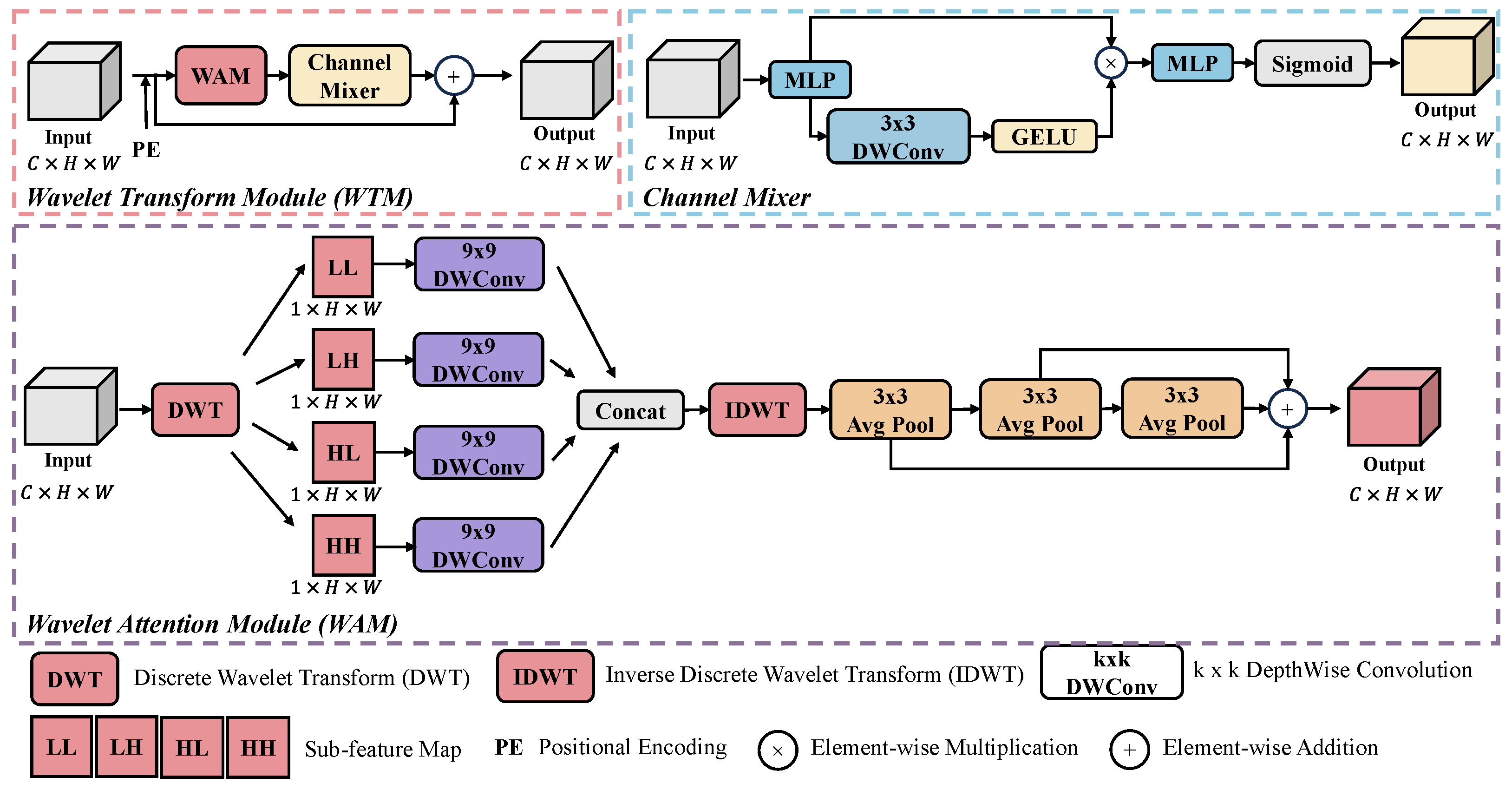
Wavelet Transform Branch: The Transformer architecture captures long-range dependencies between targets through self-attention, making it advantageous for extracting global features. However, some studies have found that the performance of Transformers is largely due to their token mixer and channel mixer frameworks. Considering that DSM images contain limited height information, we drew inspiration from GestFormer [34] and improved the multi-scale wavelet pooling Transformer. We propose a novel Wavelet Transform Module (WTM) that extracts key spatial and edge-related information. The Wavelet Transform Module consists of a Wavelet Attention Module (WAM) and a channel mixer, as shown in Figure 6. Before the Wavelet Attention Module, we introduce positional encoding. The WTM acts as a token mixer based on wavelet transform and multi-scale pooling. Additionally, we employ a convolutional gated linear unit as the channel mixer to control the flow of detailed information.

3.2.3. Wavelet Attention Module

Pooling has been shown to effectively select key features that benefit segmentation models [88]. In a similar manner, we incorporate wavelet transform to extract multi-scale features while preserving edge details, effectively mitigating the fine-grained challenges in remote sensing image segmentation. The WAM consists of two main components: a feature processing part that utilizes Discrete Wavelet Transform (DWT) and Inverse Discrete Wavelet Transform (IDWT), and a pooling mechanism for feature selection, as illustrated in Figure 6. The mathematical formulation of WAM is presented as follows:

$$F_{WAM}=F_{avgpools}\left(IDWT\left(F_{dwconvs}\left(DWT\left(X\right)\right)\right)\right)$$

(6)

where X denotes the input to WAM, DWT and IDWT represent the discrete wavelet transform and its inverse, respectively. $F_{\mathrm{dwconvs}}$ denotes the four large-kernel convolutional layers, and $F_{\mathrm{avgpools}}$ denotes the three average pooling layers.

Before applying the pooling operation, we use DWT to decompose the input into multiple sub-band features from a frequency perspective. To further enhance each sub-band feature, we employ large-kernel depthwise convolution. The DWT process can be formulated as

$$LL,LH,HL,HH=DWT\left(X\right)$$

(7)

where X represents the input feature. First, the input undergoes DWT and is decomposed into four sub-band features: LL, LH, HL, and HH. The LL component retains approximate information, while LH, HL, and HH capture horizontal, vertical, and diagonal details, respectively. These sub-band features can be categorized into low-frequency features (LL), which preserve the global structural information, and high-frequency features (LH, HL, HH), which capture edge details and local textures. Next, a $9\times 9$ depthwise convolution is applied to enhance each of the four sub-band features. The enhanced features are then concatenated and processed using Inverse Discrete Wavelet Transform to reconstruct the fused representation.

After processing with Discrete Wavelet Transform and enhancement via depthwise convolution, the transformed features are fed into a sequential pooling structure. Unlike PoolFormer, our WAM improves the original multi-scale pooling module by replacing its parallel structure with a spatial pyramid pooling design. This modification not only increases computational efficiency but also enhances the ability to aggregate multi-scale information. Our improved multi-scale pooling structure is capable of capturing features of varying sizes and shapes, effectively handling scale variations in different ground objects. Specifically, the pooling structure consists of three sequential $3\times 3$ average pooling layers, where the outputs of each pooling layer are retained, averaged together, and subsequently used as the final output of the WAM.

3.2.4. Channel Mixer

While channel attention mechanisms have played a significant role in the field of computer vision, their coarse-grained nature limits their ability to aggregate global information compared to various self-attention-based token mixers. We adopt the convolutional Gated Linear Unit (GLU) as the channel mixer to regulate the flow of channel-wise information [89], as illustrated in Figure 6. This channel mixer integrates channel attention mechanisms with a gated linear unit and further enhances positional information using depthwise convolutions to improve model stability. Compared to multilayer perceptrons, the GLU demonstrates superior performance in channel mixing. The mathematical formulation is given as follows:

$$X_M=F_m\left(X\right)$$

(8)

$$F_{CM}=\sigma \left(F_m(F_{gelu}\left(DWCon{v}_{3\times 3}\left(X_M\right)\right)\ast X_M)\right)$$

(9)

where X represents the input, $DWCon{v}_{3\times 3}$ denotes depthwise convolution with a kernel size of $3\times 3$, where the number of groups equals the number of channels. $MLP$ refers to the feed-forward neural network, $F_{gelu}$ represents the GELU activation function, and $\sigma$ denotes the Sigmoid function. After processing the input through the neural network, it is split into two parts along the channel dimension. One part undergoes depthwise convolution and GELU activation, then multiplies with the other part. The resulting product is passed through a neural network and a Sigmoid function, yielding the final output of the entire channel mixer. The Convolutional Linear GLU utilizes a gated channel attention mechanism to capture fine-grained features from the local neighborhood, adjust the channels, and enrich contextual information.

3.3. Multi-Scale Context Attention Module

Remote sensing images often contain rich details of ground objects, and the presence of multi-scale features poses significant challenges for segmentation. Combining spatial and channel attention to enhance feature representations is an effective strategy to address this issue. Inspired by the dual attention architecture [90], we propose a multi-scale context attention module that combines spatial and channel attention mechanisms. This design effectively guides the model to focus on spatially informative features, thereby improving segmentation accuracy.

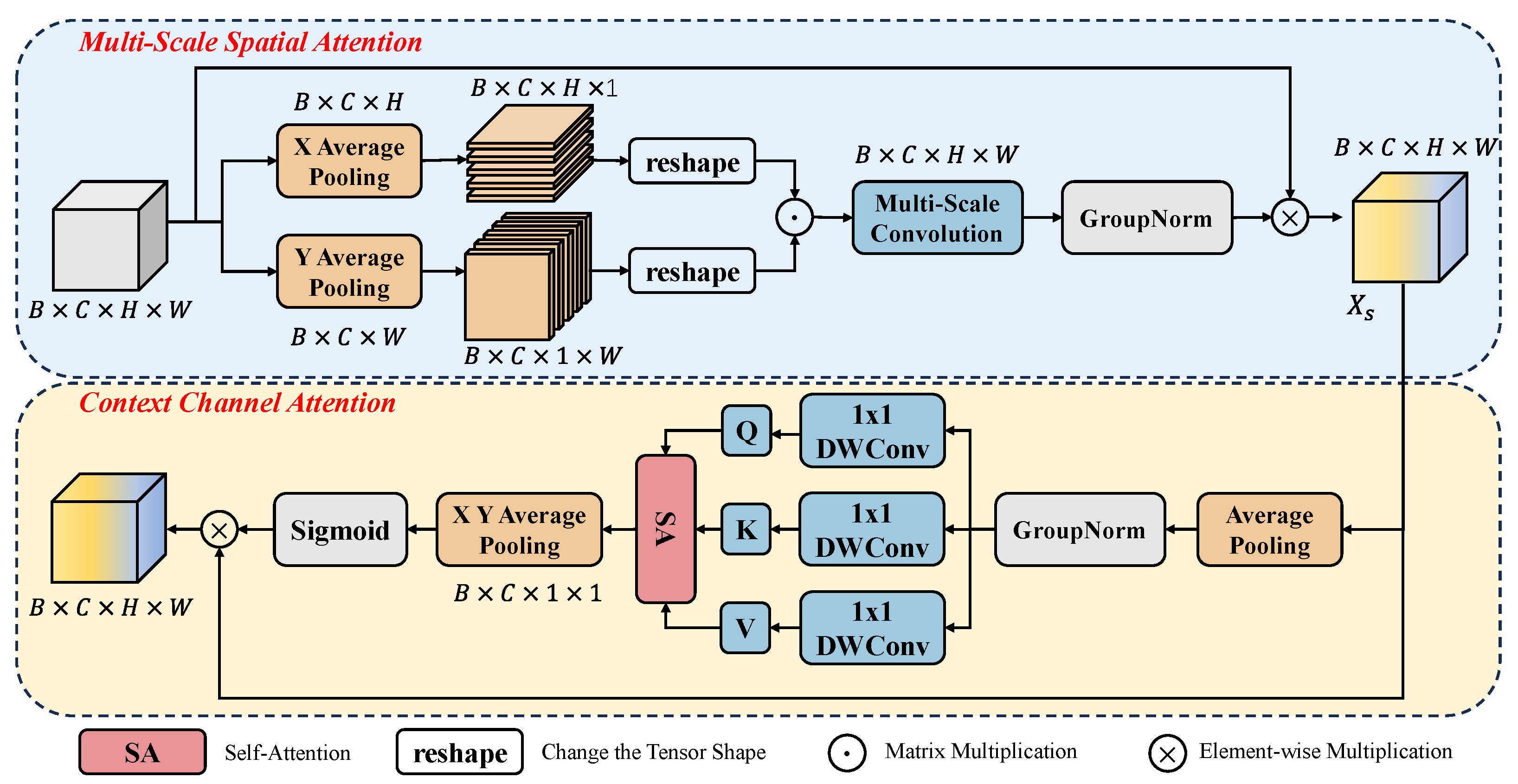
MSCAM is primarily composed of two parts: multi-scale spatial attention and contextual channel attention, with the overall structure shown in Figure 7. Some previous attention mechanisms perform average pooling and max pooling along the channel dimension to generate spatial weights for feature maps. While this method is simple and computationally efficient, it fails to capture deeper features and is prone to losing important target features. In contrast, we perform global average pooling on the input $X\in {\mathbb{R}}^{B\times C\times H\times W}$ in both the horizontal and vertical directions, obtaining two corresponding pooling results: $X_H\in {\mathbb{R}}^{B\times C\times H}$ and $X_V\in {\mathbb{R}}^{B\times C\times W}$. Then, we adjust the dimensions of both and re-multiply them to obtain the preliminary weights $X_{HV}\in {\mathbb{R}}^{B\times C\times H\times W}$.

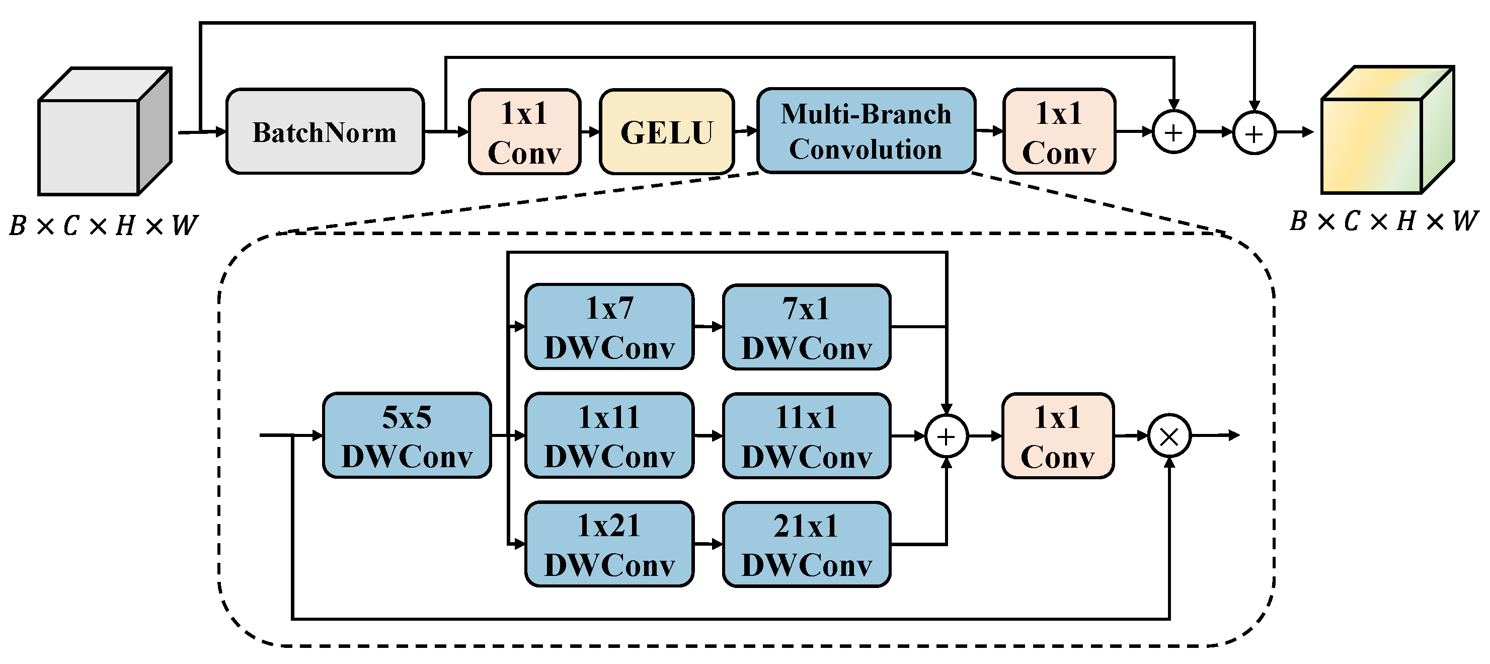
After obtaining the preliminary spatial weights, we aim to further explore the salient information in the features to prevent the loss of key features. We adopt a multi-branch deep strip convolution module to aggregate local information and capture contextual relationships, thereby enhancing the model’s ability to recognize multi-scale objects [91]. The structure of the multi-scale convolution is shown in Figure 8. We input the spatial weights $X_{HV}\in {\mathbb{R}}^{B\times C\times H\times W}$, and first process them through batch normalization, convolution, and activation functions. Then, multi-branch deep strip convolutions are applied to obtain multi-scale features, followed by a $1\times 1$ convolution to adjust the channels. Specifically, $X_B$ denotes the normalized features of $X_{HV}$; $X_{HV}^{\prime }$ represents the features obtained after applying an activation function and a pointwise convolution to $X_B$; and $X_{HV1}^{\prime }$ refers to the features produced by applying a $5\times 5$ depthwise convolution to $X_{HV}^{\prime }$. The detailed formulation is as follows:

$$X_B=BatchNorm\left(X_{HV}\right)$$

(10)

$$X_{HV}^{\prime }=F_{gelu}\left(Con{v}_{1\times 1}\left(X_B\right)\right)$$

(11)

$$X_{HV1}^{\prime }=DWCon{v}_{5\times 5}\left(X_{HV}^{\prime }\right)$$

(12)

$$\begin{array}{c}\hfill X_{HV}^{″}=\sum _{i=7,11,21}DWCon{v}_{i\times 1}\left(DWCon{v}_{1\times i}\left(X_{HV1}^{\prime }\right)\right)+X_{HV1}^{\prime }\end{array}$$

(13)

$$X_{MBC}=X_{HV}^{\prime }\otimes Con{v}_{1\times 1}\left(X_{HV}^{″}\right)$$

(14)

$$X_{MSC}=X_B+X_{MBC}+X_{HV}$$

(15)

$$X_S=X\otimes GroupNorm\left(X_{MSC}\right)$$

(16)

where i represents the kernel size for each branch in the multi-branch convolution, with values of 7, 11, and 21, respectively. ⊗ denotes the element-wise matrix multiplication. $X_{MSC}$ represents the output of the multi-scale convolution. $GroupNorm$ refers to group normalization [92]. After performing group normalization on the output $X_{MSC}$ of the multi-scale convolution, the result is multiplied element-wise by the input X to obtain the multi-scale spatial attention weights $X_S\in {\mathbb{R}}^{B\times C\times H\times W}$.

After obtaining the spatial weights, we downsample the feature map using $7\times 7$ average pooling and group normalization. Then, a $1\times 1$ depthwise convolution is applied to compute the single-head self-attention. The results are pooled over the height (H) and width (W) dimensions. Finally, channel weights are computed using the Sigmoid function. The output of the multi-scale context attention module is obtained by multiplying the spatial weights with the channel weights. The detailed formulation is as follows:

$$X_D=GroupNorm\left(AvgPoo{l}_{7\times 7}\left(X_S\right)\right)$$

(17)

$$Q=DWCon{v}_{1\times 1}\left(X_D\right)$$

(18)

$$K=DWCon{v}_{1\times 1}\left(X_D\right)$$

(19)

$$V=DWCon{v}_{1\times 1}\left(X_D\right)$$

(20)

$$X_{SA}=Softmax({\displaystyle \frac{Q{K}^T}{\sqrt{C}}})V$$

(21)

$$X_{MSCAM}=X_s\otimes \sigma \left(AvgPoo{l}_{global}\left(X_{SA}\right)\right)$$

(22)

The average pooling with a kernel size of 7 is denoted as $AvgPoo{l}_{7\times 7}$, and the result of the single-head self-attention computation is denoted as $X_{SA}$. The global average pooling operation is represented as $AvgPoo{l}_{global}$, and the final output of the multi-scale context attention module is denoted as $X_{MSCAM}$. MSCAM leverages multi-scale convolutions to capture multi-scale features and uses the self-attention mechanism to connect contextual information, further enhancing the spatial feature representation. The spatial feature processing enables the fused features to better reflect the characteristics of different targets, thereby improving the model’s performance.

3.4. Loss Function

We adopt a joint loss function to supervise the training process of our model. This joint loss is composed of the cross-entropy loss and the Dice loss, which are computed independently and then combined with equal weights. Both loss functions are widely used in semantic segmentation tasks. Their combination enhances feature learning and contributes to improved segmentation accuracy.

4. Experiments

4.1. Experimental Preparation

4.1.1. Datasets

We conducted experiments on the Vaihingen and Potsdam datasets to validate the effectiveness of our proposed method. The Vaihingen dataset is a high-resolution remote sensing image dataset captured in Vaihingen, Germany, containing 33 image patches of various sizes, each extracted from a larger true orthophoto (TOP). This TOP includes three RGB bands corresponding to near-infrared, red, and green bands. The DSM is encoded as 32-bit floating-point values, presented as grayscale images. Each TOP has a corresponding DSM, eliminating the need to consider geographic location offsets. The Vaihingen dataset represents a village scene with numerous independent and small multi-story buildings, containing six types of land cover classes: impervious surfaces, buildings, low vegetation, trees, cars, and background. Based on region indices, we split the dataset into training and testing sets. The training set consists of 16 images with the following indices: 1, 3, 5, 7, 11, 13, 15, 17, 21, 23, 26, 28, 30, 32, 34, and 37. The remaining 17 images are used for testing.

The Potsdam dataset is an ultra-high-resolution urban remote sensing image dataset featuring numerous buildings and streets. It consists of 38 image patches, each with a resolution of $6000\times 6000$, extracted from a larger true orthophoto. This TOP includes various spectral bands, with RGB images being primarily used for this study. The DSM type is consistent with that of the Vaihingen dataset. The land cover class classification is also the same as in the Vaihingen dataset. We divided the dataset into training and testing sets based on the image patch numbers. The training set consists of 24 image patches with the following numbers: 2_10, 2_11, 2_12, 3_10, 3_11, 3_12, 4_10, 4_11, 4_12, 5_10, 5_11, 5_12, 6_10, 6_11, 6_12, 6_7, 6_8, 6_9, 7_10, 7_11, 7_12, 7_7, 7_8, and 7_9. The remaining 13 images are used as the test set. Note that the image patch numbered 3_13 was found to be damaged and was excluded from both the training and testing sets.

We divide each image patch from the Vaihingen and Potsdam datasets into smaller patches, with the resulting image size being $256\times 256$ and a stride of $256\times 256$. Both datasets undergo data augmentation through horizontal and vertical flipping during training. The Vaihingen training set contains 4386 images, while the test set contains 1514 images. The Potsdam training set contains 41,472 images, and the test set contains 7488 images. The basic information of the datasets is presented in

Table 1. Summary of the datasets used in this study.

Property	ISPRS Vaihingen	ISPRS Potsdam
Image Size	$256\times 256$	$256\times 256$
Crop Stride	$256\times 256$	$256\times 256$
Train/Test Samples	4386/1514	41,472/7488
Number of Classes	6	6
Modalities	RGB + DSM	RGB + DSM

.

4.1.2. Experiment Details

We use the PyTorch (version 2.3.0) deep learning framework to train the models, running on a Linux system with a single NVIDIA GeForce RTX 4090 GPU. The AdamW [93] optimization algorithm is used for all models, with a learning rate of 0.0003, a weight decay coefficient of 0.0005, and a batch size of 16. Mosaic data augmentation [94] is employed during the training process. The number of training epochs is set to 100. The source code in this work is available at https://github.com/yhhhw/Multimodal-segmentation-network, accessed on 25 October 2025.

4.1.3. Evaluation Metrics

To better evaluate the performance of the model, we use the following metrics: Overall Accuracy (OA), mean F1 score (mF1), and mean Intersection over Union (mIoU). The specific calculation formulas are as follows:

$$\mathrm{OA}={\displaystyle \frac{TP+TN}{TP+TN+FP+FN}}$$

(23)

$$Io{U}_c={\displaystyle \frac{T{P}_c}{T{P}_c+F{P}_c+F{N}_c}}$$

(24)

$$\mathrm{mIoU}={\displaystyle \frac{1}{C}}\sum _{c=1}^{C}Io{U}_c$$

(25)

$$P_c={\displaystyle \frac{T{P}_c}{T{P}_c+F{P}_c}}$$

(26)

$$R_c={\displaystyle \frac{T{P}_c}{T{P}_c+F{N}_c}}$$

(27)

$$\mathrm{F}{1}_{\mathrm{c}}=2\times {\displaystyle \frac{P_c\times R_c}{P_c+R_c}}$$

(28)

where $TP$, $TN$, $FP$, and $FN$ represent True Positives, True Negatives, False Positives, and False Negatives, respectively. C denotes the number of classes, and mF1 represents the average of $\mathrm{F}{1}_{\mathrm{c}}$ (the F1 score for each class).

4.2. Comparative Experiment

To validate the effectiveness of the proposed model, we conduct a comprehensive comparison with eight representative segmentation methods: UNet [40], FuseNet [74], ACNet [73], ESANet [75], CMFNet [20], ASMFNet [15], FTransUNet [22], and PACSCNet [17]. All methods are evaluated on the test set under identical experimental settings.

Table 2. Comparison Experiment Results on the Vaihingen Dataset. The Bold Values Indicate the Best Performance.

Year	Method	Modality	OA (%)	mIoU (%)	mF1 (%)	F1 (%)
						ImSurf	Building	LowVeg	Tree	Car
2015	UNet [40]	Unimodal	89.51	75.13	85.18	93.20	93.03	82.04	87.30	74.35
2016	FuseNet [74]	Multimodal	91.04	81.21	89.45	94.24	94.50	83.57	89.53	85.40
2019	ACNet [73]	Multimodal	91.71	82.86	90.47	94.88	95.39	84.43	89.83	87.79
2021	ESANet [75]	Multimodal	89.70	76.94	86.60	93.17	93.18	82.21	88.17	76.24
2022	CMFNet [20]	Multimodal	90.64	80.86	89.24	93.97	94.26	82.90	89.01	86.06
2024	ASMFNet [15]	Multimodal	88.68	72.96	83.54	92.29	91.66	81.45	87.77	64.51
2024	FTransUNet [22]	Multimodal	89.65	76.47	86.24	93.25	93.10	82.45	87.97	74.41
2024	PACSCNet [17]	Multimodal	91.65	83.38	90.78	94.85	95.38	84.11	89.79	89.80
	MSFFNet	Multimodal	92.02	83.83	91.05	95.08	95.90	84.71	90.02	89.57

demonstrates that our model achieves superior performance over all compared methods, with an OA of 92.02%, mF1 of 83.83%, and mIoU of 91.05%. It exceeds ACNet by 0.31% in accuracy and outperforms PACSCNet by 0.27% in mF1. Our model achieves the best results across all five categories except for the “car” class.

Table 3. Comparison Experiment Results on the Potsdam Dataset. The Bold Values Indicate the Best Performance.

Year	Method	Modality	OA (%)	mIoU (%)	mF1 (%)	F1 (%)
						ImSurf	Building	LowVeg	Tree	Car
2015	UNet [40]	Unimodal	84.56	76.19	86.15	88.84	89.51	82.19	81.37	91.74
2016	FuseNet [74]	Multimodal	88.31	82.00	89.99	90.78	93.01	84.99	86.41	94.73
2019	ACNet [73]	Multimodal	89.90	84.61	91.51	92.57	95.55	85.87	87.77	95.80
2021	ESANet [75]	Multimodal	85.81	78.01	87.53	89.51	90.20	83.63	82.77	91.55
2022	CMFNet [20]	Multimodal	84.80	76.87	86.78	89.01	89.09	82.39	81.67	91.75
2024	ASMFNet [15]	Multimodal	85.71	77.42	87.11	89.73	90.84	82.77	80.97	91.23
2024	FTransUNet [22]	Multimodal	84.44	75.90	86.07	88.44	89.48	81.20	78.88	92.35
2024	PACSCNet [17]	Multimodal	89.99	84.61	91.55	92.65	94.51	86.97	87.94	95.69
	MSFFNet	Multimodal	90.96	85.95	92.31	93.67	96.03	87.12	88.21	96.49

shows that our model achieves superior performance in OA, mIoU, and mF1, consistently outperforming all methods across all classes. In particular, compared with the multimodal baseline PACSCNet, our model achieves improvements of 0.97% in OA, 1.34% in mIoU, and 0.76% in mF1. Compared with the single-modal U-Net method, the proposed multi-modal fusion approach provides richer information and yields more accurate segmentation results. The comparative experimental results demonstrate that our model achieves state-of-the-art performance and effectively improves segmentation accuracy.

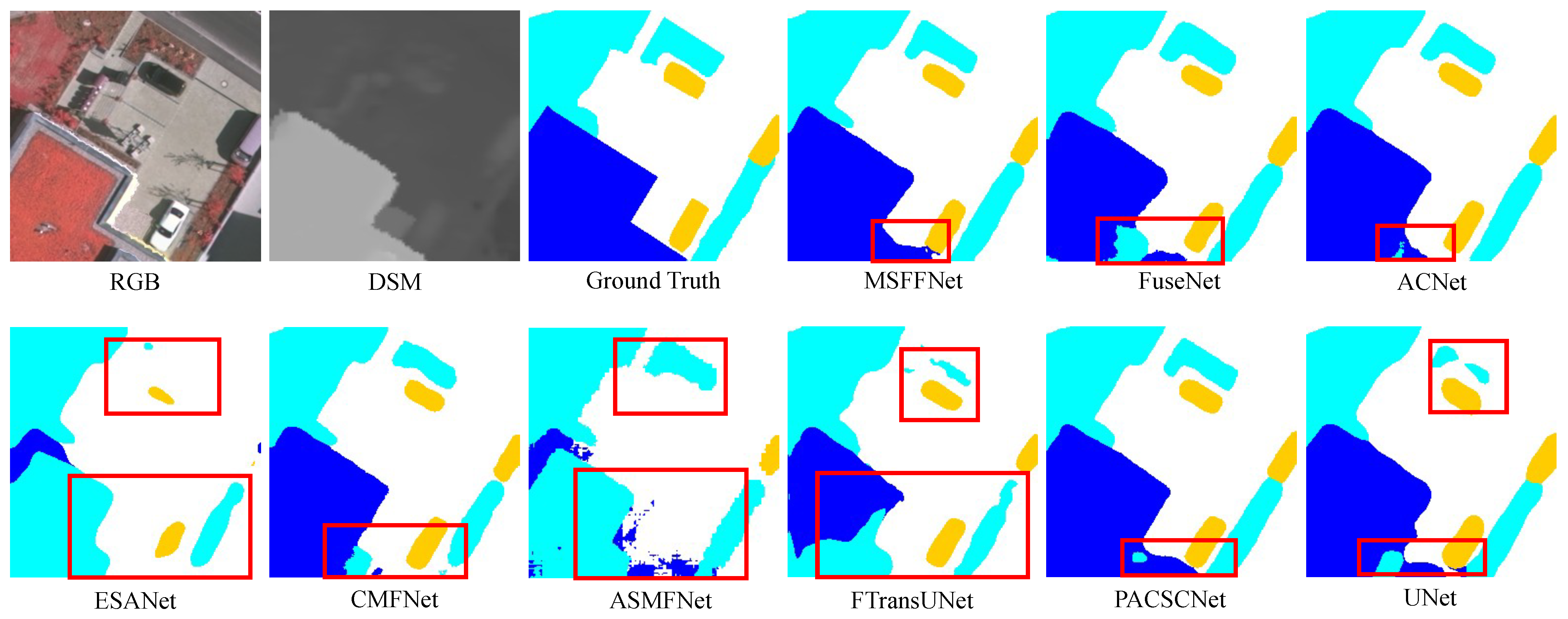
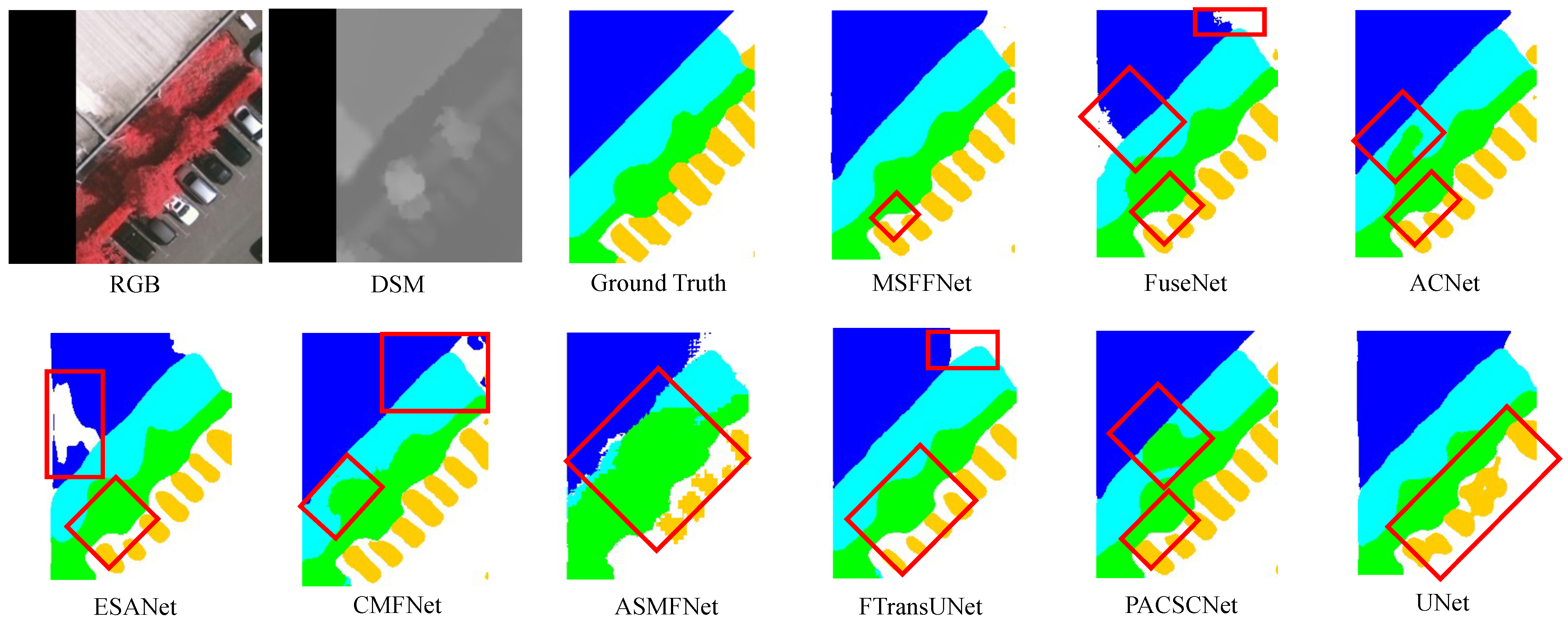
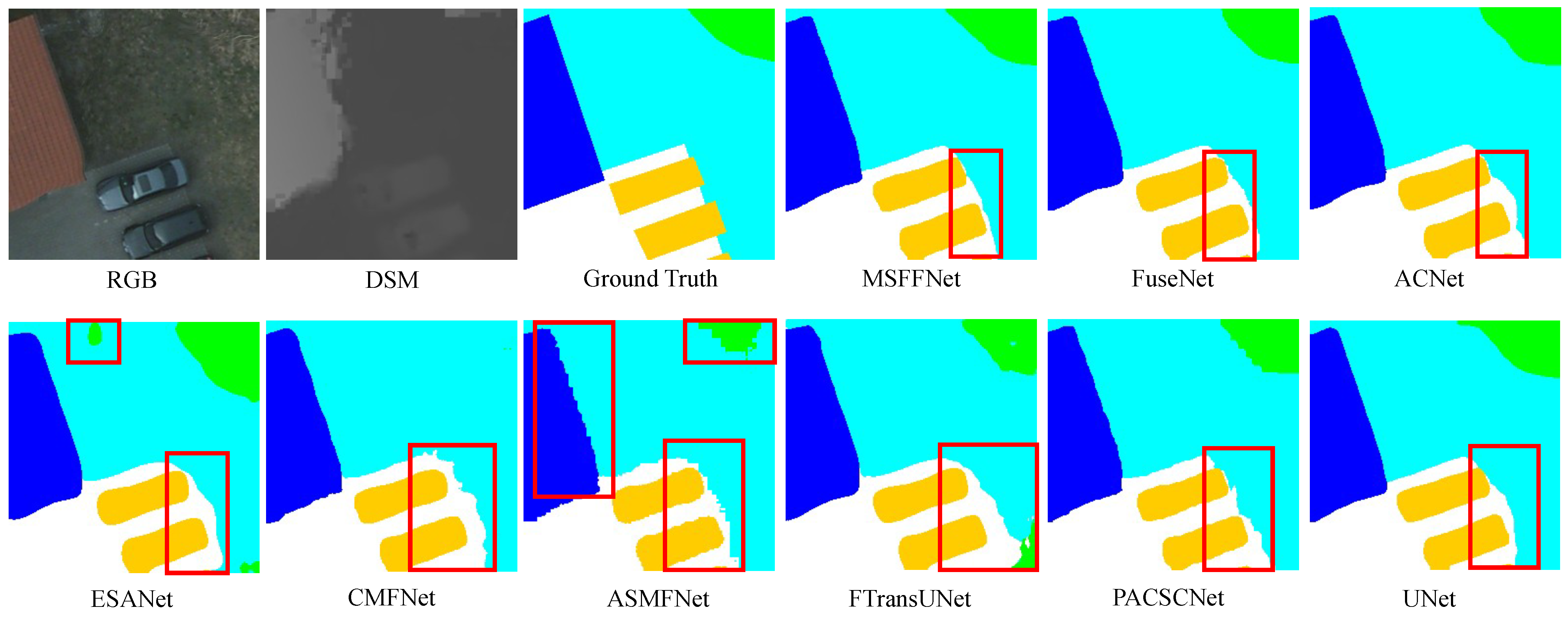
We visualized the segmentation performance of each model on the Vaihingen and Potsdam datasets, which contain objects of varying heights such as buildings, low vegetation, cars, and trees. Notable areas are marked with red boxes. In Figure 9, for Vaihingen Scene 1, the cars and other objects maintain a certain distance, and most models encounter issues at the bottom of the image. However, in terms of edge details, our model performs better than others, with contour shapes closely resembling the ground truth. In Figure 10, the difficulty in Vaihingen Scene 2 lies in distinguishing between trees, low vegetation, and dense vehicles. Our model, which incorporates DSM, preserves most of the edge information and performs the best in segmenting the objects, closely resembling the ground truth. In comparison, the majority of the other models show segmentation errors along the boundaries between trees and low vegetation.

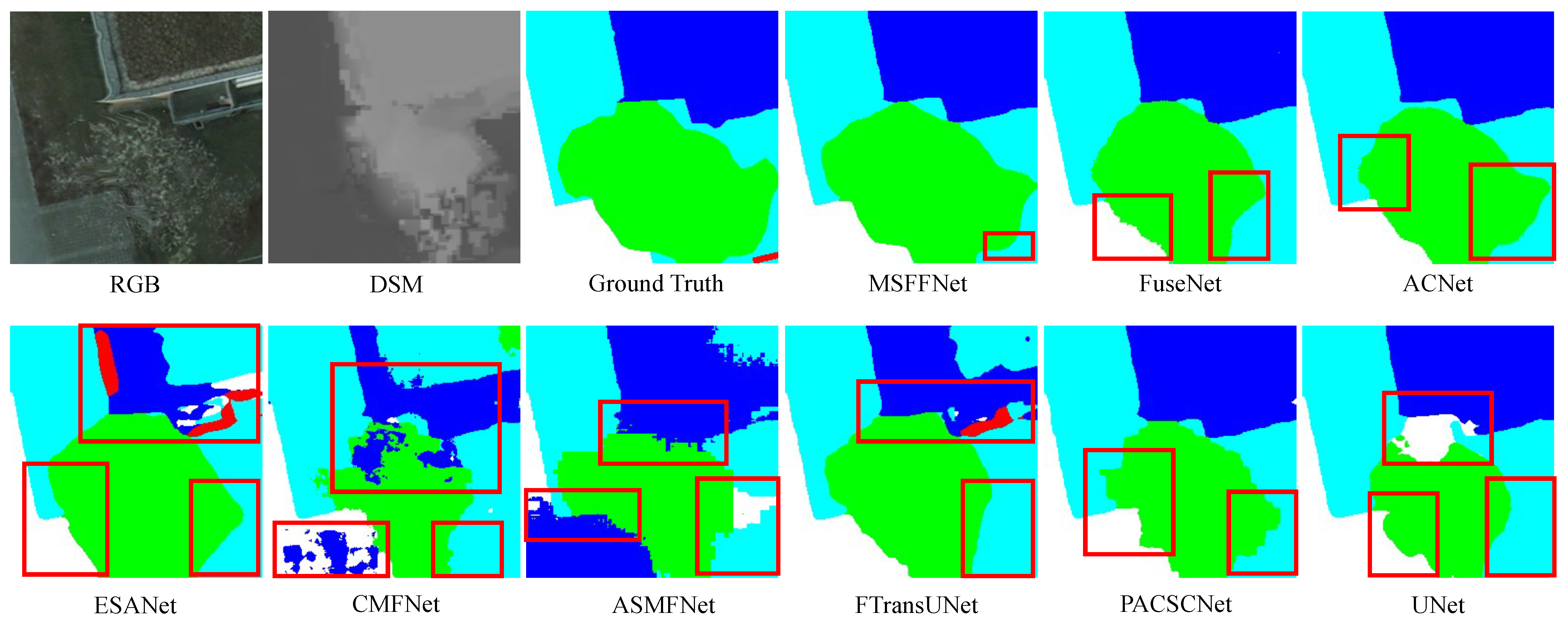
As shown in Figure 11, for Potsdam Scene 1, our model achieves the segmentation results that are most consistent with the ground truth, demonstrating the best overall performance. In contrast, other models exhibit difficulties in distinguishing between buildings and trees, as well as between trees and low vegetation. Some multimodal models, such as FTransUNet and ESANet, even misclassify certain regions into non-existent categories. In Figure 12, for Potsdam Scene 2, our model produces smoother and more accurate boundaries between cars and low vegetation compared with other methods, yielding results that are more closely aligned with the ground truth. In contrast, ASMFNet, FTransUNet, CMFNet, and ACNet show notable discrepancies in boundary-level details. Through the comparison of four scenarios, the proposed model alleviates the issue of boundary blurring and effectively enhances edge clarity.

4.3. Ablation Study

To better illustrate the impact of the designed HBFM and MSCAM, we conducted ablation experiments on the Vaihingen and Potsdam datasets. In the experiments, we use a model that replaces HBFM with a simple summation operation and removes MSCAM as the baseline. We then progressively incorporate HBFM and MSCAM into the baseline to evaluate the model’s performance at different levels of enhancement.

The ablation experiment results are shown in

Table 4. Ablation Experiments on the Vaihingen and Potsdam Datasets.“✓” Indicates that the Component Is Used, and “×” Indicates that It Is Not Used. The Bold Values Indicate the Best Performance.

Dataset	HBFM	MSCAM	OA (%)	mIoU (%)	mF1 (%)	F1 (%)
						ImSurf	Building	LowVeg	Tree	Car
Vaihingen	×	×	88.67	75.61	85.78	92.28	92.04	81.17	87.14	76.26
	✓	×	91.82	83.50	90.85	94.89	95.73	84.33	89.88	89.43
	×	✓	91.82	83.48	90.85	95.01	95.59	84.45	89.79	89.39
	✓	✓	92.02	83.83	91.05	95.08	95.90	84.71	90.02	89.57
Potsdam	×	×	87.41	80.97	89.33	91.08	92.26	83.97	85.04	94.32
	✓	×	90.80	85.80	92.22	93.50	95.98	87.11	88.42	96.12
	×	✓	89.67	83.33	90.78	92.68	95.18	85.35	87.69	93.02
	✓	✓	90.96	85.95	92.31	93.67	96.03	87.12	88.21	96.49

. On the Vaihingen dataset, when we replaced the summation operation with HBFM, the model’s performance improved. Further enhancement of the model with MSCAM resulted in a significant performance boost. The fully improved model outperformed the baseline model by 3.35%, 8.22%, and 5.27% in the three evaluation metrics, with an improvement in the F1 scores for all five categories. On the Potsdam dataset, the fully improved model achieved improvements of 3.55%, 4.98%, and 2.98% in the three metrics compared to the baseline model.

Although using HBFM alone increased the model’s accuracy, enhancing the summed features solely with MSCAM led to a decrease in performance. After analysis, we concluded that this could be due to redundancy or noise in the features resulting from the summation fusion, which posed challenges for subsequent segmentation. The fully improved model showed a reduction in performance for the “tree” category compared to the model with only the fusion enhancement, but the F1 scores for all other categories improved. In summary, the mixed-branch fusion module we designed provides higher accuracy than a simple fusion method. When combined with the multi-scale attention module, it further enhances the model’s segmentation capability.

4.4. Comparison of Fusion Methods

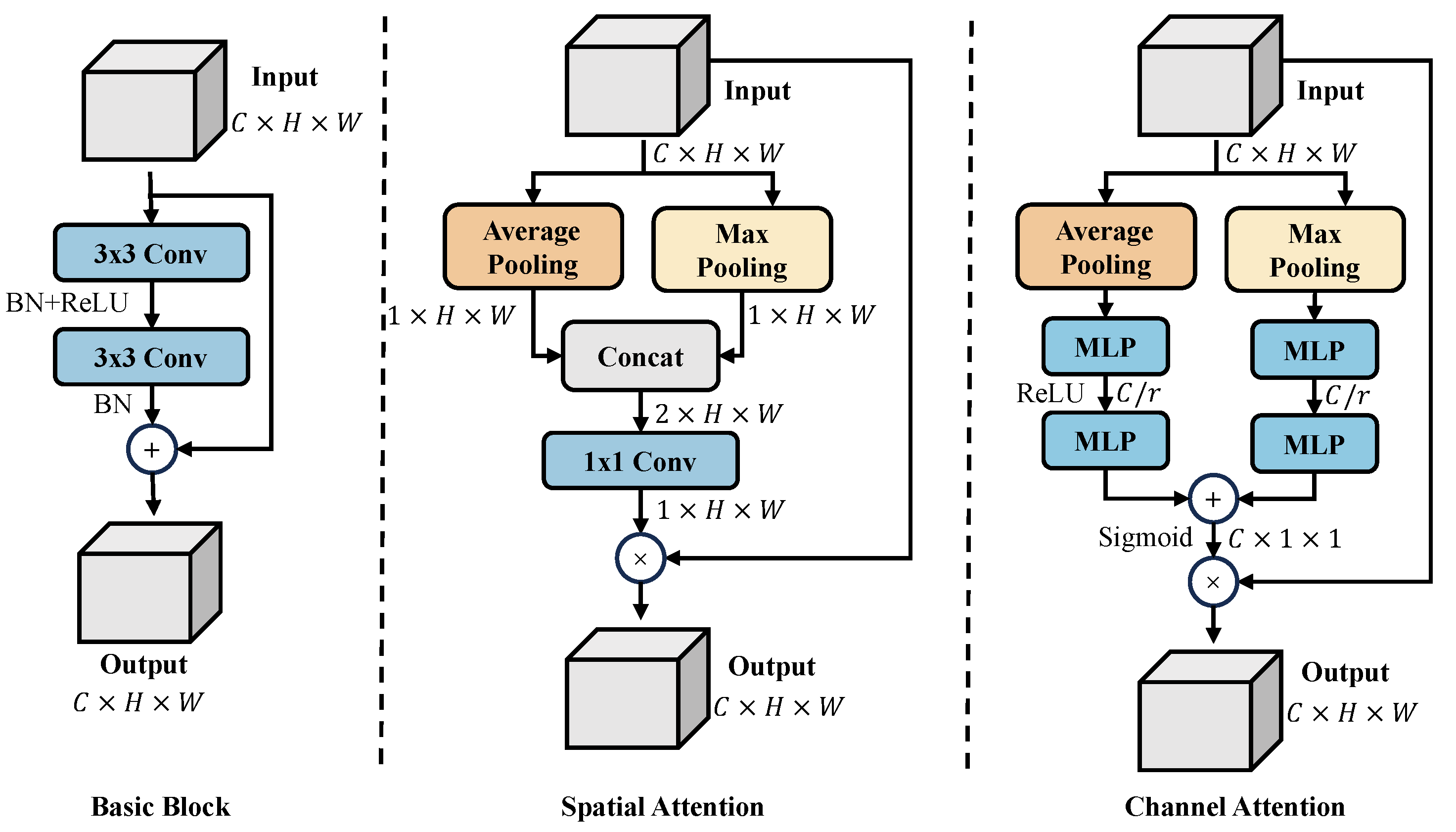
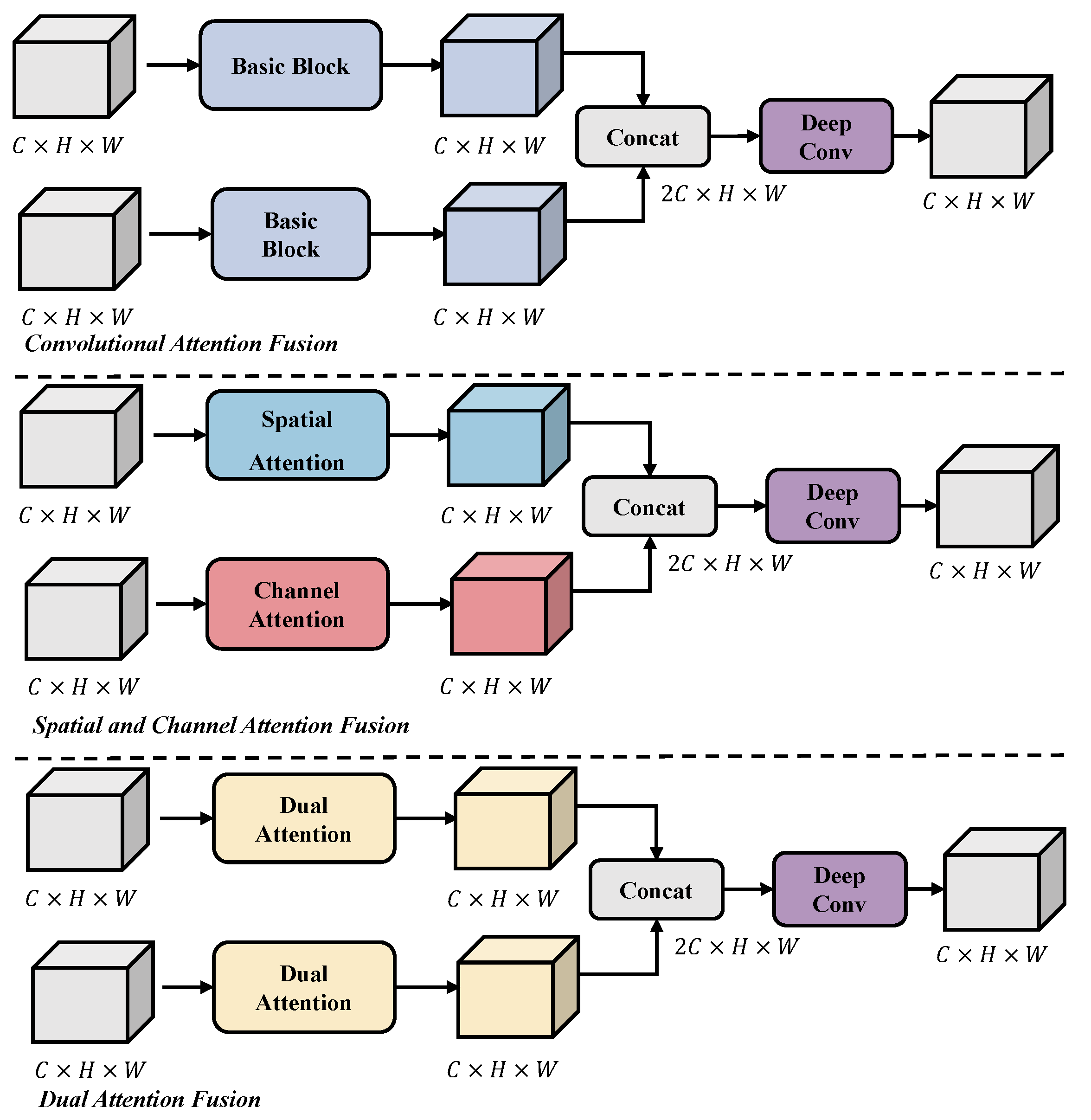
We remove MSCAM and replace HBFM with different fusion strategies to compare their impact on model performance. Specifically, we evaluate six representative fusion methods: the RGB-depth fusion module from ESANet, the iterative Attentional Feature Fusion (iAFF) from AFF [95], the Grouped Attention Gate (GAG) from UltraLightUNet [96], convolutional attention fusion, spatial and channel attention fusion, and dual attention fusion.

In the HBFM module, the convolutional attention fusion replaces the two original branches with a convolutional block composed of standard convolution, activation functions, and batch normalization. The spatial and channel attention fusion mechanisms apply average pooling and max pooling, respectively, to capture the attention weights of each branch, which are then applied to the original features, serving as substitutes for the original branches. The dual attention fusion sequentially applies spatial and channel attention operations to process the features from each branch, effectively replacing the two branches in the original HBFM. The detailed structures are illustrated in Figure 13 and Figure 14.

The experimental results are shown in

Table 5. Experimental Results of Different Fusion Methods on the Vaihingen Dataset. The Bold Values Indicate the Best Performance.

Fusion Method	OA (%)	mIoU (%)	mF1 (%)	F1 (%)
				ImSurf	Building	LowVeg	Tree	Car
ESANet fusion	91.79	83.44	90.82	94.96	95.64	84.31	89.73	89.45
iAFF	91.74	83.38	90.78	94.84	95.62	84.14	89.90	89.39
GAG	91.26	82.30	90.14	94.27	95.14	84.02	89.59	87.65
ConvAttention	91.66	83.02	90.57	94.78	95.43	84.18	89.89	88.54
SpatialChannelAttention	91.76	83.29	90.72	94.91	95.72	84.14	89.72	89.10
DualAttention	91.76	83.34	90.75	95.00	95.61	84.09	89.79	89.25
HBFM	91.82	83.50	90.85	94.89	95.73	84.33	89.88	89.43

and

Table 6. Experimental Results of Different Fusion Methods on the Potsdam Dataset. The Bold Values Indicate the Best Performance.

Fusion Method	OA (%)	mIoU (%)	mF1 (%)	F1 (%)
				ImSurf	Building	LowVeg	Tree	Car
ESANet fusion	90.61	85.49	92.04	93.29	95.82	86.97	87.93	96.17
iAFF	90.00	84.62	91.53	93.00	95.35	85.85	88.03	95.43
GAG	88.64	82.25	90.15	91.76	93.03	85.68	86.00	94.27
ConvAttention	89.81	84.22	91.33	92.39	94.20	86.64	87.94	95.45
SpatialChannelAttention	89.72	83.87	91.10	92.39	94.40	85.70	87.63	95.36
DualAttention	90.57	85.21	91.89	93.12	95.53	86.91	88.26	95.65
HBFM	90.80	85.80	92.22	93.50	95.98	87.11	88.42	96.12

. On the Vaihingen dataset, HBFM achieved the best results in OA, mIoU, and mF1. It also maintained the best performance in the segmentation of buildings and low vegetation. Although the performance for the other three categories did not reach the best, it was very close to the best-performing fusion method. On the Potsdam dataset, HBFM achieved the first-place results in all metrics except for the “car” category. These results indicate that the proposed mixed-branch fusion module effectively integrates RGB and DSM features, while preserving edge information.

4.5. Complexity Comparison

We use Floating Point Operations (FLOPs), the number of parameters, and Frames Per Second (FPS) as evaluation metrics to compare the computational complexity and inference speed of each model. FLOPs reflect the computational demands of the model, while FPS measures its inference efficiency. The experimental results are presented in

Table 7. Comparison of Computational Complexity, Parameters, and Speed. The Bold Values Indicate the Best Performance.

Method	FLOPs (G)	Parameter (M)	Speed (FPS)
UNet	55.95	26.36	402.10
FuseNet	60.36	44.17	257.40
ACNet	26.47	116.60	56.11
ESANet	8.21	34.03	80.70
CMFNet	78.26	98.49	98.49
ASMFNet	27.46	88.19	25.11
FTransUNet	56.11	179.42	8.89
PACSCNet	37.96	89.96	39.90
MSFFNet	41.64	190.84	34.79

. We employed a unified evaluation protocol to assess all the models.

Although ESANet achieves the lowest FLOPs, it exhibits relatively poor accuracy in our comparative experiments. FuseNet demonstrates the highest FPS, attributed to its simple network design; however, its performance varies significantly across datasets, indicating limited generalizability to diverse scenarios. Our proposed model does not outperform other methods in terms of FLOPs, parameter count, or FPS, ranking at a moderate level among the compared models. This is due to the inclusion of complex fusion and enhancement modules, as well as a dual-branch architecture and Transformer-based design, which increase computational overhead. Nevertheless, these components contribute to improved multimodal semantic segmentation accuracy by mitigating edge information loss during feature fusion and enhancing overall model performance.

5. Discussion

Through a series of experiments, the results show that, compared to other models, our model incorporates DSM, combines the HBFM and MSCAM, constructing a multimodal segmentation network that improves the semantic segmentation accuracy of remote sensing images. In the model comparison experiments, our model achieved excellent performance. In ablation experiments, the improvements were effective in enhancing the segmentation capabilities of the model. In scene segmentation visualization experiments, compared to other models, our model’s segmentation results were closer to the ground truth and successfully preserved edge information. We also designed different fusion strategies and tested their impact on the multimodal model. Experimental results show that, compared to other fusion strategies, HBFM achieved impressive results. On both datasets, it ranked first in OA, mIoU, and mF1.

Although our proposed model does not achieve the lowest FLOPs, parameter count, or FPS, its moderate computational complexity represents a reasonable trade-off for the substantial improvement in segmentation accuracy. The dual-branch design and Transformer-based fusion modules inevitably increase computational cost, yet they enable more effective cross-modal interaction and fine-grained feature representation. Consequently, the model attains the highest overall accuracy among all compared methods, confirming that the additional complexity is justified by its performance gains. Nevertheless, the relatively high computational demand may limit its applicability in real-time or resource-constrained scenarios. Future work will focus on enhancing model efficiency while preserving high segmentation accuracy.

6. Conclusions

This paper proposes a multimodal segmentation network that fuses RGB and DSM features, alleviating the problem of edge information loss during feature fusion and improving segmentation accuracy. We designed a Hybrid Branch Fusion Module (HBFM) that decomposes DSM features from a frequency perspective using wavelet transformations, effectively preserving edge features. This module also uses depthwise convolutions to fuse key information from RGB and DSM. Additionally, we introduced a Multi-Scale Context Attention Module (MSCAM), which combines multi-scale spatial attention and contextual channel attention sequentially to capture contextual information of the objects, enrich semantic representation, and enhance feature expressiveness. Finally, a series of experiments validated the effectiveness of the proposed method, providing a solid research foundation for semantic segmentation of remote sensing images based on multimodal feature fusion.

References

1. Liu, Y.; Zhang, Y.; Wang, Y.; Mei, S. Rethinking transformers for semantic segmentation of remote sensing images. IEEE Trans. Geosci. Remote Sens. 2023, 61, 5617515. [Google Scholar] [CrossRef]
2. Wang, Y.; Mei, S.; Ma, M.; Liu, Y.; Gao, T.; Han, H. Hyperspectral Object Tracking with Context-Aware Learning and Category Consistency. IEEE Trans. Geosci. Remote Sens. 2025, 63, 5508716. [Google Scholar] [CrossRef]
3. Wang, N.; Mei, S.; Wang, Y.; Zhang, Y.; Zhan, D. WHANet: Wavelet-Based Hybrid Asymmetric Network for Spectral Super-Resolution From RGB Inputs. IEEE Trans. Multimed. 2024, 27, 414–428. [Google Scholar] [CrossRef]
4. Wang, L.; Mei, S.; Wang, Y.; Lian, J.; Han, Z.; Chen, X. Few-Shot Object Detection with Multi-level Information Interaction for Optical Remote Sensing Images. IEEE Trans. Geosci. Remote Sens. 2024, 62, 5628014. [Google Scholar]
5. Yuan, Q.; Shen, H.; Li, T.; Li, Z.; Li, S.; Jiang, Y.; Xu, H.; Tan, W.; Yang, Q.; Wang, J.; et al. Deep learning in environmental remote sensing: Achievements and challenges. Remote Sens. Environ. 2020, 241, 111716. [Google Scholar] [CrossRef]
6. Hassan, K.A.; Elgendi, E.O.; Shehata, A.S.; Elmasry, M.I. Energy saving and environment protection solution for the submarine pipelines based on deep learning technology. Energy Rep. 2022, 8, 1261–1274. [Google Scholar] [CrossRef]
7. Guan, P.; Lam, E.Y. Cross-domain contrastive learning for hyperspectral image classification. IEEE Trans. Geosci. Remote Sens. 2022, 60, 5528913. [Google Scholar] [CrossRef]
8. Hang, R.; Yang, P.; Zhou, F.; Liu, Q. Multiscale progressive segmentation network for high-resolution remote sensing imagery. IEEE Trans. Geosci. Remote Sens. 2022, 60, 5412012. [Google Scholar] [CrossRef]
9. Yang, L.; Han, Y.; Chen, X.; Song, S.; Dai, J.; Huang, G. Resolution adaptive networks for efficient inference. In Proceedings of the IEEE/CVF Conference on Computer Vision and Pattern Recognition, Seattle, WA, USA, 14–19 June 2020; pp. 2369–2378. [Google Scholar]
10. Zheng, Z.; Yang, L.; Wang, Y.; Zhang, M.; He, L.; Huang, G.; Li, F. Dynamic spatial focus for efficient compressed video action recognition. IEEE Trans. Circuits Syst. Video Technol. 2023, 34, 695–708. [Google Scholar] [CrossRef]
11. Yang, L.; Jiang, H.; Cai, R.; Wang, Y.; Song, S.; Huang, G.; Tian, Q. Condensenet v2: Sparse feature reactivation for deep networks. In Proceedings of the IEEE/CVF Conference on Computer Vision and Pattern Recognition, Virtual, 19–25 June 2021; pp. 3569–3578. [Google Scholar]
12. Zha, J.; Fan, Y.; Li, K.; Li, H.; Gao, C.; Chen, X.; Li, Y. DIMM: Decoupled Multi-hierarchy Kalman Filter for 3D Object Tracking. arXiv 2025, arXiv:2505.12340. [Google Scholar] [CrossRef]
13. Wang, H.; Guo, R.; Ma, P.; Ruan, C.; Luo, X.; Ding, W.; Zhong, T.; Xu, J.; Liu, Y.; Chen, X. Towards Mobile Sensing with Event Cameras on High-agility Resource-constrained Devices: A Survey. arXiv 2025, arXiv:2503.22943. [Google Scholar]
14. Ma, X.; Wu, Q.; Zhao, X.; Zhang, X.; Pun, M.; Huang, B. SAM-assisted remote sensing imagery semantic segmentation with object and boundary constraints. arXiv 2023, arXiv:2312.02464. [Google Scholar] [CrossRef]
15. Ma, X.; Xu, X.; Zhang, X.; Pun, M.O. Adjacent-Scale Multimodal Fusion Networks for Semantic Segmentation of Remote Sensing Data. IEEE J. Sel. Top. Appl. Earth Obs. Remote Sens. 2024, 17, 20116–20128. [Google Scholar] [CrossRef]
16. Cui, J.; Liu, J.; Ni, Y.; Wang, J.; Li, M. FDGSNet: A Multi-modal Gated Segmentation Network for Remote Sensing Image Based on Frequency Decomposition. IEEE J. Sel. Top. Appl. Earth Obs. Remote Sens. 2024, 17, 19756–19770. [Google Scholar] [CrossRef]
17. Fan, X.; Zhou, W.; Qian, X.; Yan, W. Progressive adjacent-layer coordination symmetric cascade network for semantic segmentation of multimodal remote sensing images. Expert Syst. Appl. 2024, 238, 121999. [Google Scholar] [CrossRef]
18. Ma, X.; Zhang, X.; Pun, M.O.; Huang, B. MANet: Fine-Tuning Segment Anything Model for Multimodal Remote Sensing Semantic Segmentation. arXiv 2024, arXiv:2410.11160. [Google Scholar] [CrossRef]
19. Zheng, A.; He, J.; Wang, M.; Li, C.; Luo, B. Category-wise fusion and enhancement learning for multimodal remote sensing image semantic segmentation. IEEE Trans. Geosci. Remote Sens. 2022, 60, 4416212. [Google Scholar] [CrossRef]
20. Ma, X.; Zhang, X.; Pun, M.O. A crossmodal multiscale fusion network for semantic segmentation of remote sensing data. IEEE J. Sel. Top. Appl. Earth Obs. Remote Sens. 2022, 15, 3463–3474. [Google Scholar] [CrossRef]
21. He, S.; Yang, H.; Zhang, X.; Li, X. MFTransNet: A multi-modal fusion with CNN-transformer network for semantic segmentation of HSR remote sensing images. Mathematics 2023, 11, 722. [Google Scholar] [CrossRef]
22. Ma, X.; Zhang, X.; Pun, M.O.; Liu, M. A multilevel multimodal fusion transformer for remote sensing semantic segmentation. IEEE Trans. Geosci. Remote Sens. 2024, 62, 5403215. [Google Scholar] [CrossRef]
23. Zhang, P.; Du, P.; Lin, C.; Wang, X.; Li, E.; Xue, Z.; Bai, X. A hybrid attention-aware fusion network (HAFNet) for building extraction from high-resolution imagery and LiDAR data. Remote Sens. 2020, 12, 3764. [Google Scholar] [CrossRef]
24. Zhang, C. Based on multi-feature information attention fusion for multi-modal remote sensing image semantic segmentation. In Proceedings of the 2021 IEEE International Conference on Mechatronics and Automation (ICMA), Takamatsu, Japan, 8–11 August 2021; IEEE: New York, NY, USA, 2021; pp. 71–76. [Google Scholar]
25. Audebert, N.; Le Saux, B.; Lefèvre, S. Semantic segmentation of earth observation data using multimodal and multi-scale deep networks. In Proceedings of the Asian Conference on Computer Vision, Taipei, Taiwan, 20–24 November 2016; Springer: Berlin/Heidelberg, Germany, 2016; pp. 180–196. [Google Scholar]
26. Liu, W.; Su, F.; Jin, X.; Li, H.; Qin, R. Bispace Domain Adaptation Network for Remotely Sensed Semantic Segmentation. IEEE Trans. Geosci. Remote Sens. 2022, 60, 5600211. [Google Scholar] [CrossRef]
27. Li, J.; Han, X.H.; Qiao, X.; Sun, J.; Wang, J. DWU-Net: A Dual-Branch U-Shaped Multi-Modal Medical Image Segmentation Network Based on Wavelet Transform. In MICCAI Challenge on Comprehensive Analysis and Computing of Real-World Medical Images; Springer: Berlin/Heidelberg, Germany, 2024; pp. 240–251. [Google Scholar]
28. Zhou, Y.; Huang, J.; Wang, C.; Song, L.; Yang, G. XNet: Wavelet-Based Low and High Frequency Fusion Networks for Fully- and Semi-Supervised Semantic Segmentation of Biomedical Images. In Proceedings of the 2023 IEEE/CVF International Conference on Computer Vision (ICCV), Paris, France, 2–6 October 2023; pp. 21028–21039. [Google Scholar] [CrossRef]
29. Wang, Y.; Liu, J.; Wang, J.; Yang, L.; Dong, B.; Li, Z. HaarFuse: A dual-branch infrared and visible light image fusion network based on Haar wavelet transform. Pattern Recognit. 2025, 164, 111594. [Google Scholar] [CrossRef]
30. Wang, Z.; Liao, Z.; Wang, P.; Chen, P.; Luo, W. WaveCRNet: Wavelet Transform-Guided Learning for Semantic Segmentation in Adverse Railway Scenes. IEEE Trans. Intell. Transp. Syst. 2025, 26, 8794–8809. [Google Scholar] [CrossRef]
31. Wang, Q.; Li, Z.; Zhang, S.; Chi, N.; Dai, Q. WaveFusion: A Novel Wavelet Vision Transformer with Saliency-Guided Enhancement for Multimodal Image Fusion. IEEE Trans. Circuits Syst. Video Technol. 2025, 35, 7526–7542. [Google Scholar] [CrossRef]
32. Groenendijk, R.; Dorst, L.; Gevers, T. HaarNet: Large-scale linear-morphological hybrid network for RGB-D semantic segmentation. In Proceedings of the International Conference on Discrete Geometry and Mathematical Morphology, Florence, Italy, 15–18 April 2024; Springer: Berlin/Heidelberg, Germany, 2024; pp. 242–254. [Google Scholar]
33. Jeevan, P.; Viswanathan, K.; S, A.A.; Sethi, A. Wavemix: A resource-efficient neural network for image analysis. arXiv 2022, arXiv:2205.14375. [Google Scholar]
34. Garg, M.; Ghosh, D.; Pradhan, P.M. Gestformer: Multiscale wavelet pooling transformer network for dynamic hand gesture recognition. In Proceedings of the IEEE/CVF Conference on Computer Vision and Pattern Recognition, Seattle, WA, USA, 16–22 June 2024; pp. 2473–2483. [Google Scholar]
35. Liu, H.; Mao, Q.; Dong, M.; Zhan, Y. Infrared-visible image fusion using dual-branch auto-encoder with invertible high-frequency encoding. IEEE Trans. Circuits Syst. Video Technol. 2024, 35, 2675–2688. [Google Scholar] [CrossRef]
36. Hua, D.; Chen, Q.; Wu, Z.; Zuo, Y.; Wen, W.; Fang, Y. Perceptual Transform Fusion of Infrared and Visible Images. IEEE Trans. Circuits Syst. Video Technol. 2025. [Google Scholar] [CrossRef]
37. Wang, Z.; Zhang, Z.; Qi, W.; Yang, F.; Xu, J. FreqGAN: Infrared and visible image fusion via unified frequency adversarial learning. IEEE Trans. Circuits Syst. Video Technol. 2024, 35, 728–740. [Google Scholar] [CrossRef]
38. Vaswani, A.; Shazeer, N.; Parmar, N.; Uszkoreit, J.; Jones, L.; Gomez, A.N.; Kaiser, Ł.; Polosukhin, I. Attention is all you need. Adv. Neural Inf. Process. Syst. 2017, 30, 6000–6010. [Google Scholar]
39. Long, J.; Shelhamer, E.; Darrell, T. Fully convolutional networks for semantic segmentation. In Proceedings of the IEEE Conference on Computer Vision and Pattern Recognition, Boston, MA, USA, 7–12 June 2015; pp. 3431–3440. [Google Scholar]
40. Ronneberger, O.; Fischer, P.; Brox, T. U-net: Convolutional networks for biomedical image segmentation. In Proceedings of the Medical Image Computing and Computer-Assisted Intervention–MICCAI 2015: 18th International Conference, Munich, Germany, 5–9 October 2015; Proceedings, Part III 18; Springer: Berlin/Heidelberg, Germany, 2015; pp. 234–241. [Google Scholar]
41. Zhao, H.; Shi, J.; Qi, X.; Wang, X.; Jia, J. Pyramid scene parsing network. In Proceedings of the IEEE Conference on Computer Vision and Pattern Recognition, Honolulu, HI, USA, 21–26 July 2017; pp. 2881–2890. [Google Scholar]
42. Badrinarayanan, V.; Kendall, A.; Cipolla, R. Segnet: A deep convolutional encoder-decoder architecture for image segmentation. IEEE Trans. Pattern Anal. Mach. Intell. 2017, 39, 2481–2495. [Google Scholar] [CrossRef]
43. Chen, L.C.; Zhu, Y.; Papandreou, G.; Schroff, F.; Adam, H. Encoder-decoder with atrous separable convolution for semantic image segmentation. In Proceedings of the European Conference on Computer Vision (ECCV), Munich, Germany, 8–14 September 2018; pp. 801–818. [Google Scholar]
44. Xie, E.; Wang, W.; Yu, Z.; Anandkumar, A.; Alvarez, J.M.; Luo, P. SegFormer: Simple and efficient design for semantic segmentation with transformers. Adv. Neural Inf. Process. Syst. 2021, 34, 12077–12090. [Google Scholar]
45. Geng, J.; Song, S.; Jiang, W. Dual-path feature aware network for remote sensing image semantic segmentation. IEEE Trans. Circuits Syst. Video Technol. 2023, 34, 3674–3686. [Google Scholar] [CrossRef]
46. Li, R.; Zheng, S.; Duan, C.; Su, J.; Zhang, C. Multistage attention ResU-Net for semantic segmentation of fine-resolution remote sensing images. IEEE Geosci. Remote Sens. Lett. 2021, 19, 8009205. [Google Scholar] [CrossRef]
47. Li, Y.; Li, X.; Dai, Y.; Hou, Q.; Liu, L.; Liu, Y.; Cheng, M.; Yang, J. LSKNet: A Foundation Lightweight Backbone for Remote Sensing. arXiv 2024, arXiv:2403.11735. [Google Scholar] [CrossRef]
48. Ding, L.; Tang, H.; Bruzzone, L. LANet: Local attention embedding to improve the semantic segmentation of remote sensing images. IEEE Trans. Geosci. Remote Sens. 2020, 59, 426–435. [Google Scholar] [CrossRef]
49. Hanyu, T.; Yamazaki, K.; Tran, M.; McCann, R.A.; Liao, H.; Rainwater, C.; Adkins, M.; Cothren, J.; Le, N. Aerialformer: Multi-resolution transformer for aerial image segmentation. Remote Sens. 2024, 16, 2930. [Google Scholar] [CrossRef]
50. Wang, L.; Li, R.; Duan, C.; Zhang, C.; Meng, X.; Fang, S. A novel transformer based semantic segmentation scheme for fine-resolution remote sensing images. IEEE Geosci. Remote Sens. Lett. 2022, 19, 6506105. [Google Scholar] [CrossRef]
51. Diakogiannis, F.I.; Waldner, F.; Caccetta, P.; Wu, C. ResUNet-a: A deep learning framework for semantic segmentation of remotely sensed data. ISPRS J. Photogramm. Remote Sens. 2020, 162, 94–114. [Google Scholar] [CrossRef]
52. Ma, X.; Zhang, X.; Pun, M.O. Rs 3 mamba: Visual state space model for remote sensing image semantic segmentation. IEEE Geosci. Remote Sens. Lett. 2024, 21, 6011405. [Google Scholar] [CrossRef]
53. Wang, T.; Xu, C.; Liu, B.; Yang, G.; Zhang, E.; Niu, D.; Zhang, H. MCAT-UNet: Convolutional and cross-shaped window attention enhanced UNet for efficient high-resolution remote sensing image segmentation. IEEE J. Sel. Top. Appl. Earth Obs. Remote Sens. 2024, 17, 9745–9758. [Google Scholar] [CrossRef]
54. Zhang, J.; Shao, M.; Wan, Y.; Meng, L.; Cao, X.; Wang, S. Boundary-aware spatial and frequency dual-domain transformer for remote sensing urban images segmentation. IEEE Trans. Geosci. Remote Sens. 2024, 62, 5637718. [Google Scholar] [CrossRef]
55. Ni, Y.; Liu, J.; Chi, W.; Wang, X.; Li, D. CGGLNet: Semantic Segmentation Network for Remote Sensing Images Based on Category-Guided Global-Local Feature Interaction. IEEE Trans. Geosci. Remote Sens. 2024, 62, 5615617. [Google Scholar] [CrossRef]
56. Pastorino, M.; Moser, G.; Serpico, S.B.; Zerubia, J. CRFNet: A deep convolutional network to learn the potentials of a CRF for the semantic segmentation of remote sensing images. IEEE Trans. Geosci. Remote Sens. 2024, 62, 4707619. [Google Scholar] [CrossRef]
57. Chen, Z.; Xu, T.; Pan, Y.; Shen, N.; Chen, H.; Li, J. Edge feature enhancement for fine-grained segmentation of remote sensing images. IEEE Trans. Geosci. Remote Sens. 2024, 62, 5636613. [Google Scholar] [CrossRef]
58. Zhang, R.; Zhang, Q.; Zhang, G. LSRFormer: Efficient transformer supply convolutional neural networks with global information for aerial image segmentation. IEEE Trans. Geosci. Remote Sens. 2024, 62, 5610713. [Google Scholar] [CrossRef]
59. Wang, L.; Li, R.; Zhang, C.; Fang, S.; Duan, C.; Meng, X.; Atkinson, P.M. UNetFormer: A UNet-like transformer for efficient semantic segmentation of remote sensing urban scene imagery. ISPRS J. Photogramm. Remote Sens. 2022, 190, 196–214. [Google Scholar] [CrossRef]
60. He, X.; Liu, Y.; Zhou, Y.; Ding, H.; Zhao, J.; Liu, B.; Jiang, X. Hierarchical Relation Learning for Few-Shot Semantic Segmentation in Remote Sensing Images. IEEE Trans. Geosci. Remote Sens. 2025, 63, 4410615. [Google Scholar] [CrossRef]
61. Maiti, A.; Elberink, S.O.; Vosselman, G. TransFusion: Multi-modal fusion network for semantic segmentation. In Proceedings of the IEEE/CVF Conference on Computer Vision and Pattern Recognition, Vancouver, BC, Canada, 17–24 June 2023; pp. 6537–6547. [Google Scholar]
62. Sun, Y.; Fu, Z.; Sun, C.; Hu, Y.; Zhang, S. Deep multimodal fusion network for semantic segmentation using remote sensing image and LiDAR data. IEEE Trans. Geosci. Remote Sens. 2021, 60, 5404418. [Google Scholar] [CrossRef]
63. Du, W.L.; Gu, Y.; Zhao, J.; Zhu, H.; Yao, R.; Zhou, Y. A Mamba-Diffusion Framework for Multimodal Remote Sensing Image Semantic Segmentation. IEEE Geosci. Remote Sens. Lett. 2024, 21, 6016905. [Google Scholar] [CrossRef]
64. Gu, A.; Dao, T. Mamba: Linear-time sequence modeling with selective state spaces. arXiv 2023, arXiv:2312.00752. [Google Scholar] [CrossRef]
65. Liu, T.; Hu, Q.; Fan, W.; Feng, H.; Zheng, D. AMIANet: Asymmetric Multimodal Interactive Augmentation Network for Semantic Segmentation of Remote Sensing Imagery. IEEE Trans. Geosci. Remote Sens. 2024, 62, 5706915. [Google Scholar] [CrossRef]
66. Hong, D.; Gao, L.; Hang, R.; Zhang, B.; Chanussot, J. Deep encoder–decoder networks for classification of hyperspectral and LiDAR data. IEEE Geosci. Remote Sens. Lett. 2020, 19, 5500205. [Google Scholar] [CrossRef]
67. Mohla, S.; Pande, S.; Banerjee, B.; Chaudhuri, S. Fusatnet: Dual attention based spectrospatial multimodal fusion network for hyperspectral and lidar classification. In Proceedings of the IEEE/CVF Conference on Computer Vision and Pattern Recognition Workshops, Seattle, WA, USA, 14–19 June 2020; pp. 92–93. [Google Scholar]
68. Wang, Y.; Wan, Y.; Zhang, Y.; Zhang, B.; Gao, Z. Imbalance knowledge-driven multi-modal network for land-cover semantic segmentation using aerial images and LiDAR point clouds. ISPRS J. Photogramm. Remote Sens. 2023, 202, 385–404. [Google Scholar] [CrossRef]
69. Gao, H.; Feng, H.; Zhang, Y.; Fei, S.; Sheng, R.; Xu, S.; Zhang, B. Interactive enhanced network based on multihead self-attention and graph convolution for classification of hyperspectral and lidar data. IEEE Trans. Geosci. Remote Sens. 2024, 62, 5533716. [Google Scholar] [CrossRef]
70. Roy, S.K.; Deria, A.; Hong, D.; Rasti, B.; Plaza, A.; Chanussot, J. Multimodal fusion transformer for remote sensing image classification. IEEE Trans. Geosci. Remote Sens. 2023, 61, 5515620. [Google Scholar] [CrossRef]
71. Hong, D.; Yao, J.; Meng, D.; Xu, Z.; Chanussot, J. Multimodal GANs: Toward crossmodal hyperspectral–multispectral image segmentation. IEEE Trans. Geosci. Remote Sens. 2020, 59, 5103–5113. [Google Scholar] [CrossRef]
72. Tu, B.; Ren, Q.; Li, J.; Cao, Z.; Chen, Y.; Plaza, A. NCGLF2: Network combining global and local features for fusion of multisource remote sensing data. Inf. Fusion 2024, 104, 102192. [Google Scholar] [CrossRef]
73. Hu, X.; Yang, K.; Fei, L.; Wang, K. Acnet: Attention based network to exploit complementary features for rgbd semantic segmentation. In Proceedings of the 2019 IEEE international conference on image processing (ICIP), Taipei, Taiwan, 22–25 September 2019; IEEE: New York, NY, USA, 2019; pp. 1440–1444. [Google Scholar]
74. Hazirbas, C.; Ma, L.; Domokos, C.; Cremers, D. Fusenet: Incorporating depth into semantic segmentation via fusion-based cnn architecture. In Proceedings of the Asian Conference on Computer Vision, Taipei, Taiwan, 20–24 November 2016; Springer: Berlin/Heidelberg, Germany, 2016; pp. 213–228. [Google Scholar]
75. Seichter, D.; Köhler, M.; Lewandowski, B.; Wengefeld, T.; Gross, H.M. Efficient rgb-d semantic segmentation for indoor scene analysis. In Proceedings of the 2021 IEEE International Conference on Robotics and Automation (ICRA), Xi’an, China, 30 May–5 June 2021; IEEE: New York, NY, USA, 2021; pp. 13525–13531. [Google Scholar]
76. Li, Q.; Shen, L. Wavesnet: Wavelet integrated deep networks for image segmentation. In Proceedings of the Chinese Conference on Pattern Recognition and Computer Vision (PRCV), Shenzhen, China, 4–7 November 2022; Springer: Berlin/Heidelberg, Germany, 2022; pp. 325–337. [Google Scholar]
77. Fan, R.; Liu, Y.; Jiang, S.; Zhang, R. RGB-D indoor semantic segmentation network based on wavelet transform. Evol. Syst. 2023, 14, 981–991. [Google Scholar] [CrossRef]
78. Singh, V.K.; Kalafi, E.Y.; Wang, S.; Benjamin, A.; Asideu, M.; Kumar, V.; Samir, A.E. Prior wavelet knowledge for multi-modal medical image segmentation using a lightweight neural network with attention guided features. Expert Syst. Appl. 2022, 209, 118166. [Google Scholar] [CrossRef]
79. Anusooya, G.; Bharathiraja, S.; Mahdal, M.; Sathyarajasekaran, K.; Elangovan, M. Self-supervised wavelet-based attention network for semantic segmentation of MRI brain tumor. Sensors 2023, 23, 2719. [Google Scholar] [CrossRef]
80. Pan, W.; Shi, H.; Zhao, Z.; Zhu, J.; He, X.; Pan, Z.; Gao, L.; Yu, J.; Wu, F.; Tian, Q. Wnet: Audio-guided video object segmentation via wavelet-based cross-modal denoising networks. In Proceedings of the IEEE/CVF Conference on Computer Vision and Pattern Recognition, New Orleans, LA, USA, 18–24 June 2022; pp. 1320–1331. [Google Scholar]
81. Lin, X.; Tan, P.; Wang, Z.; Ma, L.; Li, Y. DDFL: Dual-Domain Feature Learning for nighttime semantic segmentation. Displays 2024, 83, 102685. [Google Scholar] [CrossRef]
82. Zeng, Y.; Li, J.; Zhao, Z.; Liang, W.; Zeng, P.; Shen, S.; Zhang, K.; Shen, C. WET-UNet: Wavelet integrated efficient transformer networks for nasopharyngeal carcinoma tumor segmentation. Sci. Prog. 2024, 107, 00368504241232537. [Google Scholar] [CrossRef]
83. Pan, Y.; Yong, H.; Lu, W.; Li, G.; Cong, J. Brain tumor segmentation by combining MultiEncoder UNet with wavelet fusion. J. Appl. Clin. Med Phys. 2024, 25, e14527. [Google Scholar] [CrossRef]
84. Yao, T.; Pan, Y.; Li, Y.; Ngo, C.W.; Mei, T. Wave-vit: Unifying wavelet and transformers for visual representation learning. In Proceedings of the European Conference on Computer Vision, Tel Aviv, Israel, 23–27 October 2022; Springer: Berlin/Heidelberg, Germany, 2022; pp. 328–345. [Google Scholar]
85. Shafiq, M.; Gu, Z. Deep residual learning for image recognition: A survey. Appl. Sci. 2022, 12, 8972. [Google Scholar] [CrossRef]
86. Lin, T.Y.; Dollár, P.; Girshick, R.; He, K.; Hariharan, B.; Belongie, S. Feature pyramid networks for object detection. In Proceedings of the IEEE Conference on Computer Vision and Pattern Recognition, Honolulu, HI, USA, 21–26 July 2017; pp. 2117–2125. [Google Scholar]
87. Liu, Z.; Mao, H.; Wu, C.Y.; Feichtenhofer, C.; Darrell, T.; Xie, S. A convnet for the 2020s. In Proceedings of the IEEE/CVF Conference on Computer Vision and Pattern Recognition, New Orleans, LA, USA, 18–24 June 2022; pp. 11976–11986. [Google Scholar]
88. Yu, W.; Luo, M.; Zhou, P.; Si, C.; Zhou, Y.; Wang, X.; Feng, J.; Yan, S. Metaformer is actually what you need for vision. In Proceedings of the IEEE/CVF Conference on Computer Vision and Pattern Recognition, New Orleans, LA, USA, 18–24 June 2022; pp. 10819–10829. [Google Scholar]
89. Shi, D. Transnext: Robust foveal visual perception for vision transformers. In Proceedings of the IEEE/CVF Conference on Computer Vision and Pattern Recognition, Seattle, WA, USA, 16–22 June 2024; pp. 17773–17783. [Google Scholar]
90. Si, Y.; Xu, H.; Zhu, X.; Zhang, W.; Dong, Y.; Chen, Y.; Li, H. SCSA: Exploring the synergistic effects between spatial and channel attention. arXiv 2024, arXiv:2407.05128. [Google Scholar] [CrossRef]
91. Guo, M.H.; Lu, C.Z.; Hou, Q.; Liu, Z.; Cheng, M.M.; Hu, S.M. Segnext: Rethinking convolutional attention design for semantic segmentation. Adv. Neural Inf. Process. Syst. 2022, 35, 1140–1156. [Google Scholar]
92. Wu, Y.; He, K. Group normalization. In Proceedings of the European Conference on Computer Vision (ECCV), Munich, Germany, 8–14 September 2018; pp. 3–19. [Google Scholar]
93. Loshchilov, I.; Hutter, F. Decoupled weight decay regularization. arXiv 2017, arXiv:1711.05101. [Google Scholar]
94. Bochkovskiy, A.; Wang, C.Y.; Liao, H.Y.M. Yolov4: Optimal speed and accuracy of object detection. arXiv 2020, arXiv:2004.10934. [Google Scholar] [CrossRef]
95. Dai, Y.; Gieseke, F.; Oehmcke, S.; Wu, Y.; Barnard, K. Attentional feature fusion. In Proceedings of the IEEE/CVF winter Conference on Applications of Computer Vision, Virtual, 5–9 January 2021; pp. 3560–3569. [Google Scholar]
96. Rahman, M.M.; Marculescu, R. UltraLightUNet: Rethinking U-shaped Network with Multi-kernel Lightweight Convolutions for Medical Image Segmentation. Preprint on OpenReview. 2025. Available online: https://openreview.net/forum?id=BefqqrgdZ1 (accessed on 15 October 2024).
Figure 1. Examples of the Potsdam dataset. From left to right, the images are the remote sensing RGB image, the corresponding DSM image, and the ground truth. The DSM represents different heights using grayscale values.
Remotesensing 17 03745 g001
Figure 2. The structure of the proposed method. RGB and DSM images are first downsampled to obtain low-resolution features, which are then processed by ResNet to extract multi-scale representations. HBFM and MSCAM perform fusion and enhancement of RGB and DSM features.
Remotesensing 17 03745 g002
Figure 3. The structure of HBFM.
Remotesensing 17 03745 g003
Figure 4. Comparison of feature maps after fusion in the first stage of the encoder. The shallow feature maps reflect the quality of the fused features, where the hybrid method produces representations that are closer to the original image. The visualizations use a color spectrum to represent activation intensity, where bright yellow denotes the highest activations, green represents intermediate values, and dark blue signifies the lowest or zero activations.
Remotesensing 17 03745 g004
Figure 5. The structure of Deep Convolution (DeepConv) Fusion (a) and ConvNeXt Block (b).
Remotesensing 17 03745 g005
Figure 6. The structure of the WTM. The Wavelet Transform Module (WTM) consists of a Wavelet Attention Module (WAM) and a Channel Mixer. After positional encoding, the input is separately processed by the two submodules, followed by a residual connection to obtain the final output of the WTM. The WAM is composed of Discrete Wavelet Transform (DWT), Inverse Discrete Wavelet Transform (IDWT), and multiple average pooling layers for edge information extraction. The Channel Mixer includes linear layers, convolutional operations, and activation functions to regulate the information flow.
Remotesensing 17 03745 g006
Figure 7. The structure of the MSCAM. The MSCAM consists of a Multi-Scale Spatial Attention submodule and a Contextual Channel Attention submodule. In the first submodule, the horizontally and vertically pooled features are processed by multi-scale convolutions, followed by group normalization to generate spatial attention weights. Based on these spatial attention weights, a self-attention mechanism is further applied to produce the final output of the MSCAM.
Remotesensing 17 03745 g007
Figure 8. The structure of the Multi-Scale Convolution.
Remotesensing 17 03745 g008
Figure 9. Visualizationcomparison experiment on Vaihingen Scene 1. The color mapping for each class follows the scheme defined in Figure 1.
Remotesensing 17 03745 g009
Figure 10. Visualization comparison experiment on Vaihingen Scene 2.
Remotesensing 17 03745 g010
Figure 11. Visualization comparison experiment on Potsdam Scene 1.
Remotesensing 17 03745 g011
Figure 12. Visualization comparison experiment on Potsdam Scene 2.
Remotesensing 17 03745 g012
Figure 13. The structural diagrams of convolutional attention fusion, spatial and channel attention fusion.
Remotesensing 17 03745 g013
Figure 14. The structural diagrams of the three fusion modules.
Remotesensing 17 03745 g014