Article

Graph-Based Multi-Resolution Cosegmentation for Coarse-to-Fine Object-Level SAR Image Change Detection

1
Key Laboratory of Target Cognition and Application Technology (TCAT), Aerospace Information Research Institute, Chinese Academy of Sciences, Beijing 100190, China
2
Aerospace Information Research Institute, Chinese Academy of Sciences, Beijing 100094, China
3
School of Electronic, Electrical and Communication Engineering, University of Chinese Academy of Sciences, Beijing 100049, China
4
College of Surveying and Geo-Informatics, Tongji University, Shanghai 200092, China
*
Author to whom correspondence should be addressed.
Remote Sens. 2025, 17(22), 3736; https://doi.org/10.3390/rs17223736
Submission received: 16 September 2025 / Revised: 4 November 2025 / Accepted: 12 November 2025 / Published: 17 November 2025
(This article belongs to the Special Issue SAR Image Change Detection: From Hand-Crafted to Deep Learning)

Highlights

What are the main findings?
  • We propose a novel SAR change detection framework based on multi-level structural feature embedding and graph consistency analysis.
  • This method is robust to speckle noise and improves the detection ability of small-scale targets while maintaining the structural integrity of the changing region.
What are the implications of the main findings?
  • This method provides a modeling approach for capturing the spatially correlated structural relationships among analysis units at different scales within the image.
  • This method enhances the accuracy and efficiency of SAR image change detection in large-scale and complex scenes.

Abstract

The ongoing launch of high-resolution satellites has led to a significant increase in the volume of synthetic aperture radar data, resulting in a high-resolution and high-revisit Earth observation that efficiently supports subsequent high-resolution SAR change detection. To address the issues of speckle noise interference, insufficient integrity of change targets and blurred boundary location of high-resolution SAR change detection, we propose a coarse-to-fine framework based on the multi-scale segmentation and hybrid structure graph (HSG), which consists of three modules: multi-scale segmentation, difference measurement, and change refinement. First, we propose a graph-based multi-resolution co-segmentation (GMRCS) in the multi-scale segmentation module to generate hierarchically nested superpixel masks. And, a two-stage ranking (TSR) strategy is designed to help GMRCS better approximate the target edges and preserve the spatio-temporal structure of changed regions. Then, we introduce a graph model and measuring difference level based on the HSG. The multi-scale difference image (DI) is generated by constructing the HSG for bi-temporal SAR images and comparing the consistency of the HSGs to reduce the effect of speckle noise. Finally, the coarse-scale change information is gradually mapped to the fine-scale based on the multi-scale fusion refinement (FR) strategy, and we can get the binary change map (BCM). Experimental results on three high-resolution SAR change detection datasets demonstrates the superiority of our proposed algorithm in preserving the integrity and structural precision of change targets compared with several state-of-the-art methods.

1. Introduction

Change detection (CD) is one of the key researches in the field of remote sensing earth observation, aimed at analyzing and extracting change information by comparing satellite images taken at different times in the same scene [1]. Various image sources, including optical, multispectral, thermal infrared and synthetic aperture radar (SAR), have been applied in practice. Compared with passive observation sensing mode, SAR can transmit clouds and provide all-day and all-weather earth observation. It is widely used in change detection applications, such as urban development [2,3,4], environmental monitoring [5,6], disaster management [7,8] and situational awareness [9,10]. However, due to its unique side-looking and coherent imaging mechanism, SAR images have severe speckle noise and geometric distortion, which poses a great challenge to SAR image change detection [11].
Change detection typically involves three stages: (1) image co-registration, (2) difference image (DI) generation, and (3) change map (CM) production. Since most multi-temporal SAR data are Level-1 products, co-registration and DEM-based ortho-correction are required [12,13,14]. The data used here have been pre-registered; thus, this study focuses on DI and CM generation. Traditional SAR change detectors include ratio-based, region-based, and fusion-driven methods [15,16,17,18]. Recently, graph-based approaches have emerged as effective solutions [19,20], modeling pixel or object relations [21] and measuring changes via graph similarity to suppress speckle noise. With the growing resolution of SAR imagery, object-based and deep learning techniques have become increasingly valuable for reducing imaging interference and improving feature representation in high-resolution change detection.
Object-based change detection (OBCD) segments SAR images into homogeneous regions and computes change features at the superpixel level, effectively reducing errors from speckle noise in high-resolution data. Numerous studies have demonstrated the superiority of object-based over pixel-based methods [22,23,24,25]. Fu et al. [22,26] reported 3–10% higher accuracy in wetland vegetation mapping using object-based techniques. Wan et al. [23] developed a multi-scale statistical model employing Kullback–Leibler divergence to reduce false alarms, while Wan et al. [24] introduced a SAR-specific distance metric to enhance change discrimination. To extend these advantages to high-resolution SAR imagery, Zhu et al. [25] proposed a coarse-to-fine framework using multi-scale joint segmentation and uncertainty modeling to progressively extract changed objects. In recent years, the Segment Anything Model (SAM) has attracted widespread attention as a powerful image segmentation approach. It can extract homogeneous foreground regions from images in an unsupervised manner and has demonstrated remarkable advantages in various remote sensing applications. For example, Xue et al. [27] designed an adapter module for SAM to dynamically refine feature representations and enhance ship detection performance.
Recently, deep learning-based change detection (DLCD) has shown remarkable performance in SAR imagery by autonomously learning robust and discriminative features [28]. Gao et al. [29] introduced PCANet to extract neighborhood features for direct change mapping, and later proposed a convolutional wavelet neural network (CWNN) for sea ice monitoring [30]. Zhang et al. [31] further enhanced CWNN using multi-level superpixel fusion and fuzzy clustering to detect small changes. Qu et al. [32] developed a dual-domain network (DDNet) integrating spatial–frequency features, while Zhang et al. [33] incorporated attention mechanisms with a ViT-like model to capture long-range dependencies. Xie et al. [34] addressed high-frequency loss via a wavelet-based aggregation network. Additionally, object-based deep learning frameworks have been explored, such as Zhang et al.’s two-phase approach (TPOBDL) [35] and Ji et al.’s siamese U-Net model [36], which integrate segmentation and deep learning for refined change localization. Ai et al. [37] subsequently proposed MKSFF-CNN, which introduces a multi-channel parallel topology convolution architecture that greatly enhances the completeness of SAR target feature representation.
Despite the groundbreaking advancements of deep learning (DL) methods in SAR change detection (CD), several challenges remain [38]. Most DL-based SAR change detection methods rely on pseudo-labeled samples generated by pre-classification [39], where label noise can degrade network performance [40,41]. Although numerous optimization strategies have been proposed [42,43,44], the impact of label noise persists. Moreover, the training inputs for DLCD networks are usually local rectangular image blocks, making it difficult to extract target-level semantic information [45]. While some studies have adapted network structures and training paradigms to accommodate irregular objects [36,46], challenges still exist. Furthermore, current DLCD methods face challenges in directly applying to very high-resolution (VHR) SAR images due to the limited annotated samples [25]. This is because VHR SAR images experience stronger speckle noise and intense scattering fluctuations, hindering DLCD methods from extracting effective deep features. Moreover, geometric distortions from side-looking imaging, such as layover, double-bounce effects, and shadowing in non-informative regions also exacerbate change detection false alarms [17]. The vast majority of DLCD methods have been evaluated on medium- and low-resolution SAR images, and their performance on VHR SAR images has yet to be fully investigated. Since DLCD methods are trained using local square patches, their ability to extract complex content from SAR images is restricted, preventing them from mitigating the interference induced by the characteristics of high-resolution imaging [47].
Overall, deep learning (DL) has revolutionized the field of remote sensing, often outperforming most traditional approaches in specific scenarios and datasets. However, for high-resolution SAR images, due to the inherent characteristics of speckle noise, object-based image analysis (OBIA) remains a reliable and effective solution. In this paper, we propose a change detection method for high-resolution SAR images based on a multi-level hybrid structural graph (HSG). The main contributions of this work are summarized as follows:
(1)
A graph-based multi-resolution co-segmentation (GMRCS) method is proposed, which is guided by a two-stage ranking (TSR) strategy of edges. This approach jointly segments bi-temporal SAR images to generate hierarchically nested superpixel masks while effectively preserving the structural information of change regions.
(2)
A hybrid structural graph is constructed to represent multi-level spatial relationships within the SAR image, integrating pixel–pixel, pixel–region, and region–region connections. Change intensity is quantified from the perspective of graph structural consistency, effectively mitigating the impact of speckle noise.
(3)
A region-level fusion refinement model is developed to integrate change information across multiple segmentation scales. By progressively propagating coarse-scale changes to finer levels, this strategy maintains the spatial integrity of change regions and enhances the detection of small-scale variations.
The rest of this article is organized as follows. Section 2 outlines the details of the proposed method. Section 3 covers the experimental designs, experimental results, and analysis. Finally, Section 4 concludes this article.

2. Methodology

Figure 1 illustrates the workflow of the proposed method, which consists of three main modules: (1) GMRCS, the graph-based multi-resolution co-segmentation module, which generates multi-scale superpixel masks using a two-stage ranking strategy; (2) HSG, the hybrid structural graph change measurement module, which constructs multi-level spatial relationships at the superpixel scale and quantifies change intensity via graph structural consistency; (3) FR, the multi-scale fusion refinement module, which integrates change results across scales to enhance the completeness of change regions and preserve fine details.

2.1. Graph-Based Multi-Resolution Co-Segmentation

Graph-based multi-resolution co-segmentation (GMRCS) is a segmentation method designed for change detection tasks, addressing the lack of effective and fast multi-temporal segmentation methods in object-level change detection. GMRCS represents an image as a graph, where the nodes represent pixels, the edges represent connections between pixels or regions, and the edge weights represent the similarity between adjacent regions. GMRCS then traverses each edge and merges regions that meet the merging criterion.
(1) Multi-resolution co-segmentation: Previously, we proposed multi-resolution joint segmentation (MRJS) [25] for SAR images change detection. The MRJS is based on the minimum heterogeneity criterion (MHR) of the fractional net evolution approach (FNEA). MHR integrates spectral and shape heterogeneity features, which are defined as follows:
h = ω c o l o r × h c o l o r + ω s h a p e × h s h a p e
where h c o l o r and h s h a p e denotes the spectral and shape heterogeneity increment, respectively. ω s p e c t r a l and ω s h a p e are the weights of spectral and shape components, and ω s p e c t r a l + ω s h a p e = 1 . They are defined as
h s p e c t r a l = c ω c × n r i r j × σ r i r j ω c × n r i × σ c , r i + n r j × σ c , r j
h s h a p e = ω s m o o t h × h s m o o t h + ω c o m p × h c o m p
where ω c is the weight of c-band, n r i , n r j and n r i r j denote the number of pixels of the i-th and j-th and merged parcels. σ c , r i , σ c , r j and σ c , r i r j are the standard on c-band. Usually, c ω c = 1 . h s m o o t h and h c o m p denote smoothness and compactness heterogeneity, respectively, as defined in the study [25].
Considering the single image segmentation, the adjacent regions are merged when the heterogeneity increment h meets h < T , T is the pre-defined threshold. Considering multi-temporal segmentation in the change detection task, we can define two merging thresholds T p r e and T p o s t for the bi-temporal SAR image, respectively. And then, we can get the overall heterogeneity increment h p r e and h p o s t resulting from the merging of adjacent regions in I p r e and I p o s t , respectively. If the following conditions are simultaneously satisfied
h p r e < = T p r e h p o s t < = T p o s t
the adjacent regions on I p r e and I p o s t are merged.
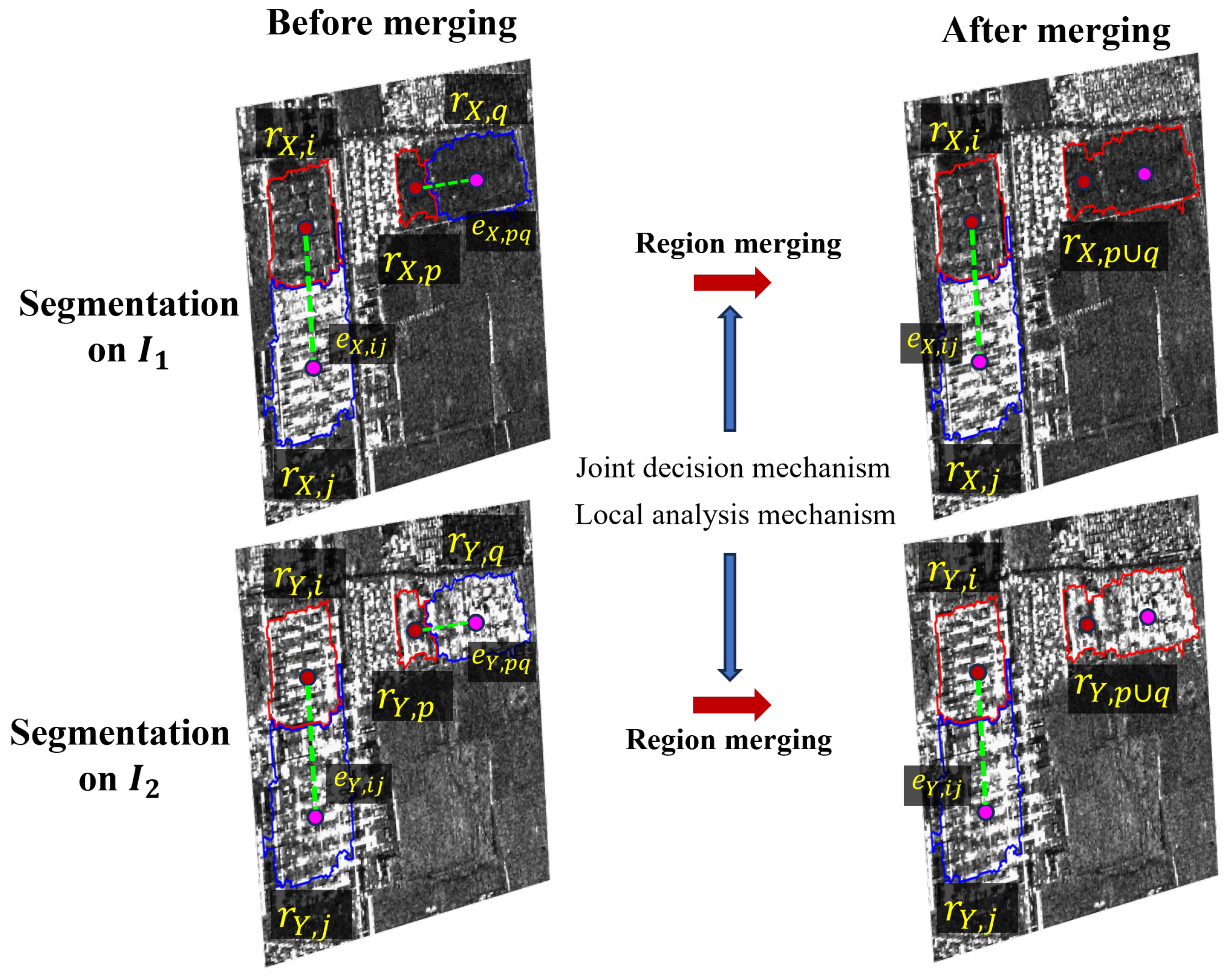
The advantage of co-segmentation lies in establishing segmentation correlations between different images, thereby preserving the changed areas structure during segmentation. This prevents the loss of change information due to excessive regional merging during Object-Based Image Analysis (OBIA). Figure 2 illustrates the co-segmentation process. In the figure, the regional characteristics of r X , p and r X , q are similar, while those of r Y , p and r Y , q are also similar. The heterogeneity of edges e X , p q and e Y , p q is below the predefined merging threshold, thus satisfying the merging conditions. Thus, in the merged result, r X , p and r X , q merge into r X , p q , while r Y , p and r Y , q merge into r Y , p q . However, although r Y , i and r Y , j are similar to each other and meet the merging criteria, they are not merged because the heterogeneity between r X , i and r X , j is too high, failing to satisfy the joint decision mechanism (denoted as Equation (4)). In traditional single image segmentation, r Y , i and r Y , j might be merged, potentially obscuring areas of change. Under the co-segmentation framework, the local heterogeneity of I p r e and I p o s t is simultaneously considered. This allows change regions (i.e., locations of r X , i and r Y , i ) to be individually preserved in the final segmentation result, effectively reducing the possibility of change region misclassification.
(2) Graph-based co-segmentation strategy: Multi-resolution segmentation (FNEA) starts with a single pixel and merges neighboring pixels in bottom-up order. This merging order often suffers from redundancy and poor segmentation timeliness. Therefore, we use a graph-based strategy to construct GMRCS. The graph-based segmentation strategy assumes the SAR image as an undirected weighted graph G = ( V , E ) , V and E denote the vertex sets and edge sets, are defined as V = { v 1 , v 2 , , v N } and E = { e 1 , e 2 , , e M } , respectively.
For a SAR image, each pixel can be represented by a vertex, and each edge e k = ( u , v ) possesses a weight ω ( u , v ) , which is the dissimilarity between vertices u and v. In order to generate homogeneous primitive for SAR images, the vertex V needs to be divided into K mutually disjoint components, i.e., superpixels, objects, regions, or parcels. Each superpixel corresponds to a connected subgraph G = ( V , E ) , where V V and E E . Superpixel can be expressed using a minimum spanning tree (MST). A spanning tree (ST) is defined as a weighted, undirected, acyclic subgraph, and the MST is actually the spanning tree with the least total weight of all connected edges among vertices [48]. Thus, graph-based segmentation can be viewed as the process of obtaining the MST of a SAR image. This is because the pixels within the MST have the least overall dissimilarity, resulting in a local region with fairly similar attributes.
The Kruskal algorithm is one of the commonly used methods for extracting MST, which is a greedy algorithm. It first ranks all edges by their weight in ascending order and processes them starting from the smallest, deciding whether to merge adjacent nodes based on specific segmentation criterion (e.g., intra-regional consistency or MHR, etc.), and then gradually generates a local region (subgraph). Notably, Kruskal algorithm integrates naturally with segmentation criteria due to its edge-guided MST construction, making it computationally efficient.
In a single segmentation scenario, a SAR image can be modeled as a graph G = ( V , E ) , where the edge weights are defined as
ω ( i , j ) = m a x c I p r e , c ( v i ) I p o s t , c ( v j )
where I p r e , c and I p o s t , c denote the node intensity of dual-temporal images on c-band. The edge E can be easily ranked, and then we can extract homogeneous parcels by kruskal algorithm. In the co-segmentation scenario, we will build two edge sets E p r e and E p o s t , and how to rank them and incorporate them into graph-based framework remains unclear. To address the problem of ranking associated edges across I p r e and I p o s t , we propose a Two-Stage Ranking (TSR) method to adapt to the co-segmentation tasks.
In co-segmentation, graph can be constructed for each bi-temporal images, defined as follows:
G p r e = ( V p r e , E p r e ) , G p o s t = ( V p o s t , E p o s t )
where e p r e , k E p r e , e p o s t , k E p o s t ( k = 1 , , M ) denote the k-th edge in I p r e and I p o s t , respectively. First, the Formula (5) is used to assign weights to the initial edge sets E p r e and E p o s t , denoted respectively as
ω p r e : E p r e R + , ω p o s t : E p o s t R +
The objective of the two-stage ranking is to obtain an optimized set of edge pair indexes (EPI), defined as
Q = T E p r e , E p o s t , ω p r e , ω p o s t
where T ( · ) denotes the TSR operation, which returns the sorted edge pair index set Q = { q k } k = 1 M , where q k corresponds to the position index of the edge pair e p r e , k , e p o s t , k in the new edge set. The sorting process can be decomposed into two stages:
T ( · ) = S F ( E p r e , E p o s t , ω p r e , ω p o s t )
where, F ( · ) represents the First Stage Ranking (FSR), while S ( · ) denotes the Second Stage Ranking (SSR).
The first-stage ranking F ( · ) is defined as
E ^ p r e , E ^ p o s t = F E p r e , E p o s t , ω p r e , ω p o s t = R a n k e i j E ω p r e ( i , j ) + ω p o s t ( i , j )
where, R a n k e i j E denotes the ascending order of edge weights, E ^ p r e , E ^ p o s t represents the edge pair indices after the first-stage sorting, and E ^ p r e and E ^ p o s t denote the sorted edge sets respectively. The FSR prioritizes merging adjacent nodes with high similarity. Therefore, the algorithm should first process edge pairs with the smallest weights to ensure the rationality and coherence of region merging.
Second-stage ranking (SSR) further optimizes the FSR and is defined as follows:
E ˜ p r e , E ˜ p o s t = S E ^ p r e , E ^ p o s t , ω ^ p r e , ω ^ p o s t = R a n k e i j E ^ | ω ^ p r e ( i , j ) ω ^ p o s t ( i , j ) |
where ω ^ p r e and ω ^ p o s t denote the edge weights after FSR, while E ˜ p r e , E ˜ p o s t represents the final edge pair index set after SSR. The core idea of SSR is to further rank the results from the FSR based on the difference in edge weights between the pre- and post-time. By prioritizing the merging of edges with similar weights, SSR effectively prevents change regions from being merged into large-scale regions, thereby preserving the structure of these change regions.
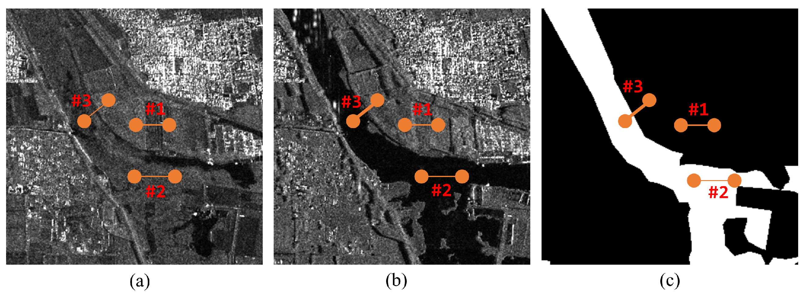
Figure 3 illustrates the core considerations of the two stage ranking method to meet the requirements of change detection tasks. In the figure, #1, #2, and #3 represent the three edge pairs ( e # 1 , p r e , e # 1 , p o s t ) , ( e # 2 , p r e , e # 2 , p o s t ) , and ( e # 3 , p r e , e # 3 , p o s t ) , respectively. The width of the lines indicates the weight of the corresponding edges. It can be observed that the two nodes of e # 1 , p r e reside within the same homogeneous region, resulting in a smaller edge weight. Similarly, the two nodes of e # 1 , p o s t also belong to the same homogeneous region, yielding a smaller weight. Since the regions containing e # 1 , p r e and e # 1 , p o s t remain unchanged, this region should be prioritized for merging during the partitioning process. For e # 2 , p r e and e # 2 , p o s t , although their regions have changed, they remain within the same homogeneous area with similar weights. Therefore, this region should also be prioritized for merging. In contrast, observing ( e # 3 , p r e , e # 3 , p o s t ) reveals a significant weight disparity between these two edges. This indicates that either ( e # 3 , p r e ) or ( e # 3 , p o s t ) resides in a heterogeneous region, which may undergo changes. Therefore, merging this region should be postponed until the partitioning process stabilizes.
(3) Hierarchical co-segmentation masks: Based on the scale of the units to be merged at the start of segmentation, we decomposes GMRCS into two merging stages and performs hierarchical segmentation across L levels, with the segmentation threshold increment between levels defined as T s + 1 = T s + Δ . The first segmentation stage begins at the pixel level (hierarchical scale l = 1 ). Utilizing Formula (5), a pixel-level graph model is constructed. After traversing all edge pairs in the edge set Q , the first-stage segmentation mask is obtained, denoted as Ω 1 = { r 1 , r 2 , , r N } is obtained. The second stage begins with Ω 1 and performs segmentation at scales l = 2 to l = L . Since the segmentation units at this stage are primitives with relatively large dimensions, we employ statistical distance to measure similarity between adjacent regions. The edge weight can be defined by spectral histograms, as follows:
ω ( r i , r j ) = c d i s t ( h c , i , h c , j )
where, d i s t ( h c , i , h c , j ) is the χ 2 function. The second stage involves constructing region adjacency graphs (RG) in the dual-phase SAR image domains I p r e and I p o s t , denoted as R G p r e and R G p o s t , respectively. After constructing the region adjacency graphs, the TSR strategy is similarly applied to jointly rank the edge sets, thereby optimizing the merging order for the Kruskal algorithm.
Figure 4 illustrates the overall workflow of the graph-based multi-resolution co-segmentation proposed in this paper. GMRCS comprises two segmentation stages: the first stage segments images into homogeneous primitives starting from pixels, while the second stage merges small-scale primitives into larger-scale regions starting from homogeneous primitives, thereby modeling hierarchical structures to capture multi-scale features.

2.2. Hybrid Structure Graph Change Detector

In order to suppress the interference of high-frequency scatter and ensure the completeness of the change information, we adopt a robust method based on the affinity relationship to detect the degree of change. Inspired by the hierarchical heterogeneity graph (HHG) [49], we propose constructing a hybrid structure graph HSG of SAR images and measuring the changes based on the degree of consistency of the HSG of the anterior and posterior time-phase images.
Hybrid Structure Graph (HSG) is defined as a graph structure containing nodes and edges, denoted as H S G = { V , E , ω } . HSG effectively captures the local structural features of an image through affinity relations. We construct the affinity relations of HSG at the pixel level, region level, and the mixing level of pixels and regions, respectively, including the pixel-level affinity, region-level affinity, and the mixing affinity between pixels and regions, which characterize the similarity between nodes in the graph. In HSG, V denotes the set of nodes in the graph, including pixel nodes and region nodes; E denotes the set of connected edges between nodes; and W denotes the weights of connected edges. Based on the theoretical framework of HHG [49], we define HSG formally as follows:
V = V p V R ; E = E p p E r r E r p E p r E p r p ; E p p = { ( p n , p k ) : p n , p k V p , p k K L N N ( p n ) } ; E r r = { ( r n , r k ) : r n , r k V R , r k E S ( r n ) } ; E r p = E p r = { ( r n , p k ) : r n V R , p k V p , p k r n } ; E p r p = { ( p n , p k ) : p n , p k V p , r m   and   p k K P T N ( r m ) }
where p n , p k denote pixel nodes, r n , r k denote region nodes, V P and V R are sets of pixel nodes and region nodes, and E p p , E r r , E r p , E p r and E p r p are different types of edges in the graph, respectively. K L N N ( · ) , E S ( · ) and K P T N ( · ) denote different connectivity rules, respectively.
E p p is the set of pixel-pixel connected edges, which is constructed based on the location nearest rule (K-location nearest neighbor, KLNN) and expresses the affinity relationship at the pixel level. For a pixel p i on an image, the set of spatially neighboring pixels is denoted as K L N N s ( p i ) , and the size of the neighborhood window is s × s . In order to suppress the scattering noise, we use the patch-based non-iterative probability weights shown below to express the similarity:
ω p p ( p i , p j ) = exp 1 K k N w I ( p i , k ) I ( p j , k ) + I ( p j , k ) I ( p i , k )
where p j K L N N s ( p i ) , the patch size is w × w , K = w × w , and w is usually set to 3.
E r r is the set of connected edges between region nodes, which is constructed based on the Edge Sharing (ES) rule and expresses the affinity relationship between regions. For each region r i in the partition mask, the affinity with neighboring regions is calculated as follows:
ω r r ( r i , r j ) = h , q Φ exp I ( p h ) I ( p q ) 2
where p h r i ,   p q r j , and ϕ denotes the edges shared by regions r i and r j , p h and p q are the pixel nodes connected by the shared edges contained in r i and r j , respectively, and I ( · ) denotes the SAR magnitude value.
E r p and E p r are the edges between pixel and region, and it express the affinity relationship between pixels and regions. In HSG, E r p and E p r are equivalent and defined as follows:
ω p r ( p i , r j ) = ω r p ( r j , p i ) = 1 , if p i r j 0 , if others
E r p and E p r express the containment relationship between pixels and regions.
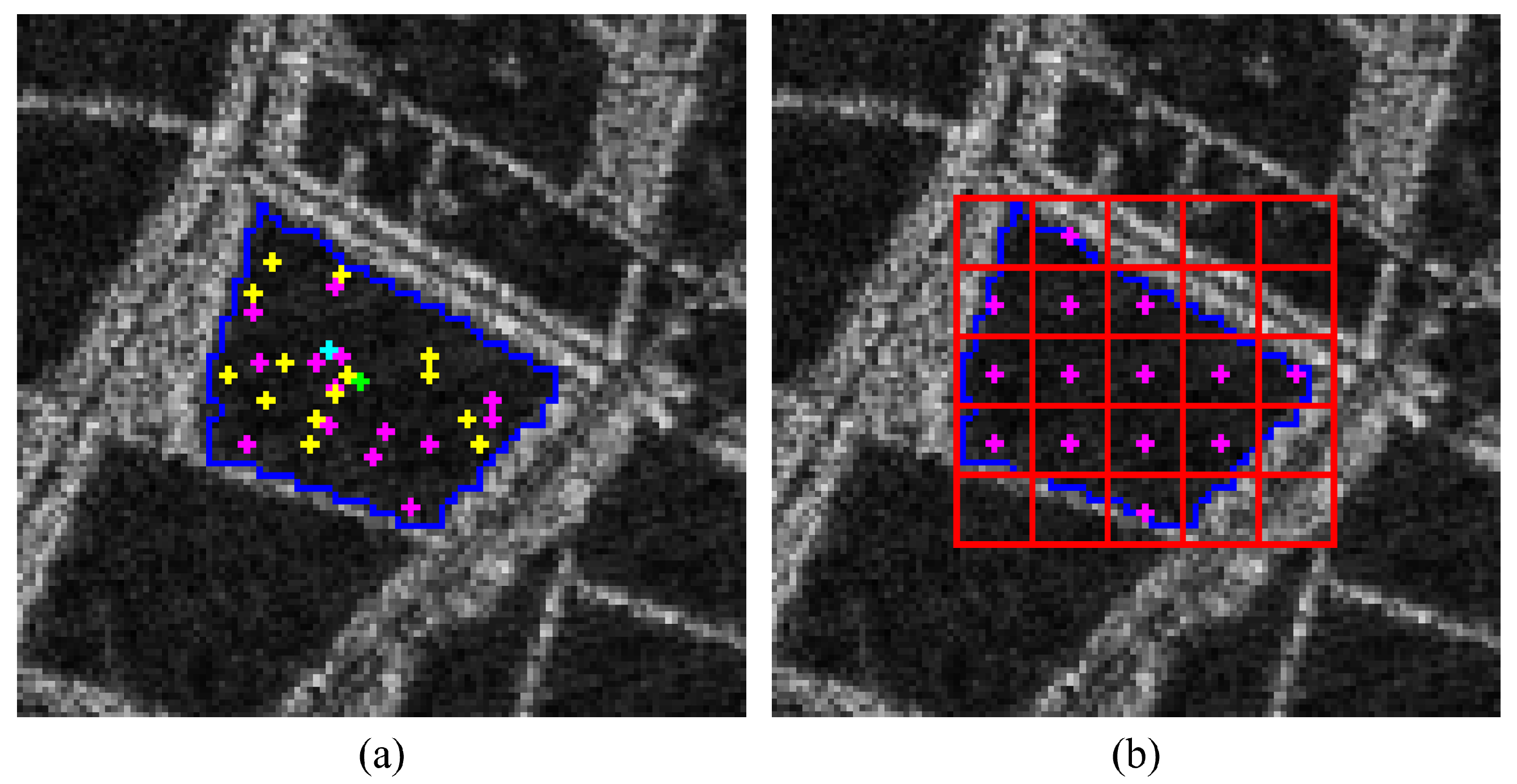
E p r p represents a mixed affinity relationship between a pixel and a region, based on the connection between the pixel and the regional key pixel, differing from E r p and E p r . The K-Nearest Neighbors (KNN) rule can be employed to search for pixels within the region that exhibit similar intensity values to the target pixel [49], and these are then designated as the basis for constructing E p r p . However, due to repeated searches, this method incurs a high computational cost. To address this, we propose a grid-based key point extraction method (GKPE). For a region r i , we uniformly divide its minimum bounding rectangle into r g r i d × r g r i d grids, and using the grid centers as candidate key points. The candidate points within r i are selected as key points. As shown in Figure 5, our method eliminates repetitive searches [(a)] by using grid centers to predefine key points [(b)], where red lines represent grid divisions, and pink points denote selected key pixels.
For pixel p i , we are able to extract K region keypoints p l K P T N ( r j ) in the region r j to which it belongs, and thus the mixing affinity relationship between the pixel and the region can be expressed by the patch similarity calculation of p i and p l
ω p r p ( p i , p j ) = exp 1 K k N w I ( p i , k ) I ( p i , k ) + I ( p j , k ) I ( p i , k )
According to edge sets, the affinity matrix W can be derived, which quantifies the key information and local structure of SAR image, and W is defined as
W = ω ( i , j ) , i f i , j E 0 , o t h e r w i s e
furthermore, the degree matrix and the random wandering matrix are defined as D i i = j W i j and P = D 1 W , respectively. Assuming that the intensity and mean intensity characteristics of the pixels and the region nodes are defined as F P = { f p ( i ) R , i = 1 , , N } and F R = { f r ( i ) R , i = 1 , , M } , respectively, which in turn can be used to describe the key properties on the graph by the following equation:
( P f ) ( i ) = 1 i , j E ω ( i , j ) i , j E ω ( i , j ) f ( j )
where ( P f ) ( i ) describes the concentration of information from neighboring nodes to the study node i. It can be viewed as an on-graph filter, which suppress scattering noise. Based on the E = { E p p , E r r , E r p , E p r , E p r p } , we are able to obtain P = { P p p , P r r , P p r , P r p , P p r p } , which in turn enables us to derive the hybrid structure graph (HSG) of the SAR image. The HSG incorporates both regional and pixel-level information and can be defined as follows:
H S G = λ × H S G r e g i o n + ( 1 λ ) × H S G p i x e l = P p r ( P r r f r + P r p f p ) + ( P p p + P p r p ) f p
where, region-level information H S G r e g i o n is conveyed through P r r , P p r , P r p , while pixel-level information H S G p i x e l is conveyed by P p p , P p r p . λ is the smoothing parameter, which adjusts the weight between H S G r e g i o n and H S G p i x e l to achieve a balance between speckle suppression and local detail preservation. f p represents the intensity features of pixel nodes, while f r denotes the regional node and average intensity features. By leveraging hierarchical connectivity, regional features can be propagated to the pixel scale, fully utilizing spatial contextual information to suppress speckle noise. Constructing H S G p r e and H S G p o s t on I p r e and I p o s t , respectively, enables the generation of a Pixel Level Difference Image (PLDI) based on the following metric:
P L D I = log H S G p r e log H S G p o s t

2.3. Region-Level Fusion Refinement Model

Assuming that GMRCS generates L segmentation masks for I p r e and I p o s t , according to HSG (Equation (21)), then we can construct the multiscale difference images P L D I = { P L D I 1 , P L D I 2 , , P L D I L } , in which each DI reflects the change information of the scale. By fusing the L difference maps, we significantly improve the accuracy and robustness of change detection. Firstly, the P L D I is converted to a region-level change information, and the change intensity of each region is the average of the change intensities of the pixels contained in that region, so we can obtain L region-level difference images (RLDI) with R L D I = { R L D I 1 , R L D I 2 , R L D I L } . Then, we classify each RLDI using FCM to obtain the membership degree matrix (MDM) at l scale, denoted as U l = u 1 , c u N l , c u 1 , u c u N l , u c , U l R 2 × N l . Subsequently, a fusion matrix derived based on spectral and distance similarities is used to fuse the coarse scale results { R L D I 2 , , R L D I L } to the finest scale R L D I 1 . Specifically, at each coarse scale, we compute a fusion matrix M l R N l × N 1 , for l = 2 , , L . Each element in M l can be computed by the following equation:
M i , j = N 1 , i N l , j exp d i s t A m p ( r 1 , i , r l , j ) + d i s t L o c ( r 1 , i , r l , j ) 2 β
where N 1 , i and N l , j denote the number of pixels contained in the regions r 1 , i and r l , j , respectively, and d i s t A m p denotes the magnitude feature similarity, which is obtained by calculating the euclidean distance between the spectral features of r 1 , i and r l , j . d i s t L o c denotes the positional feature similarity, which is obtained by calculating the euclidean distance between the centers of the two regions, and β is usually set to 0.5.
After obtaining the fusion matrix M = { M 2 , M 3 , , M L } for each coarse scale, we can project U 2 , U 3 , , U L to the finest scale U 1 , which in turn yields the refined region-level MDM. The fusion process is represented as follows:
R U = U 1 + U 2 M 2 + U 3 M 3 + + U L M L
where R U = u 1 , c u N 1 , c u 1 , u c u N 1 , u c denotes the refined MDM. Finally, we get the final change map based on the following judgment:
C M ( r 1 , i ) = 1 , i f u i , c > u i , u c 0 , i f u i , c u i , u c
The proposed RMF-HSG integrates pixel, region, and cross-layer affinity relationships within a unified framework, improving the robustness of DI by measuring the consistency of bi-temporal HSG.

3. Experimental Results and Analysis

In this section, we validate the effectiveness of the proposed algorithm using three pair of SAR datasets. First, we compare the proposed method with several state-of-the-art approaches from the aspects of visual and quantitative indicators. Then, the ablation studies and parameters analysis are conducted. Finally, we compare the segment anything-based change detection.

3.1. Experiment Dataset Description

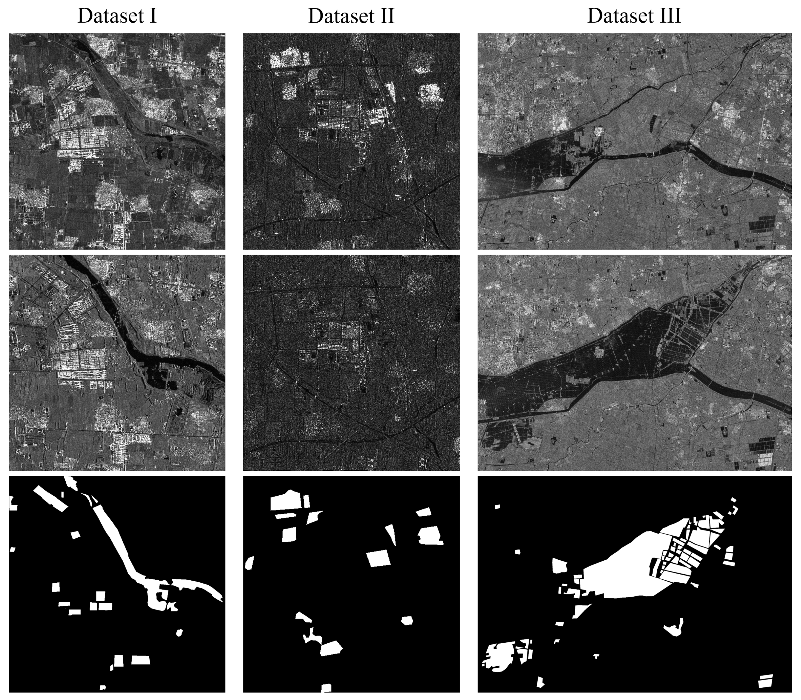
In this study, we used three real SAR image pairs, named Dataset I, Dataset II, and Dataset III, as shown in Figure 6. A brief description of each dataset is provided below.
  • Dataset I: This dataset includes two TerraSAR images, each with a size of 1000 × 1000 pixels, acquired in January 2014 and August 2015, HH polarization, 3 m resolution, StripMap mode, ENL ≈ 6.3. The high-resolution images capture changes in water bodies and buildings between the two observations.
  • Dataset II: The two GF-3 images (600 × 600 pixels) acquired in July and August 2023, HH polarization, 10 m resolution, Fine StripMap mode, ENL ≈ 1.6, used for flood-related building change detection in Zhou Zhou, Hebei, China, following a flood event.
  • Dataset III: This dataset covers a different geographic area from DatasetĨI within the same imaging task. The images have a size of 1965 × 2848 pixels, HH polarization, 10 m resolution, Fine StripMap mode, and ENL ≈ 5.7. This region captures significant post-flood surface changes in a floodplain in Hebei, including farmland inundation and waterbody expansion.

3.2. Comparison Methods and Parameter Setting

We selected seven state-of-the-art methods for comparison with our proposed method, including SBMRF [50], NLSW [21], HHG [49], CoSEG-BCD [51], LANTNet [43], SAFNet [52], DDNet [32], CAMixer [33], and AEKAN [53]. These comparison methods cover various popular types in recent years. SBMRF, a segmentation-based change detection method capable of preserving complete change features, was configured with parameters set as: β ranging from 4 to 9, and the number of superpixels K = 3000 . NLSW and HHG are graph-based change detection methods. For NLSW, we set the parameters as: ω 1 = 2 , ω 2 = 7 , k = 0.1 , L = 1 . For HHG, we set the parameters as: K s = 2 , K r = 1 , K c = 10 % . For the four self-supervised (or unsupervised) deep learning methods, they are configured with the parameters settings suggested in original paper. For proposed RMF-HSG, we set ω s p e c t r a l = 0.7 , ω s m o o t h n e s s = 0.7 , L = 10 , the initial threshold T p r e t i m e = T p o s t t i m e = 10 , Δ = 10 , ω = 3 , and r g r i d = 5 . Notably, the thresholds T p r e t i m e and T p o s t t i m e can be set to different values according to the scene characteristics, land cover type and the degree of interference of the dual-temporal SAR image.

3.3. Evaluation Criteria

The evaluation indicators are derived from four key elements of the confusion matrix: T P , F P , T N , and F N . Assume that the ground truth contains N c actual changed pixels, and N n c unchanged pixels. Thus, T P (True Positive) is the number of pixels in the intersection of the detected foreground and the labeled foreground. T N (True Negative) is the number of pixels in the intersection of the detected background and the labeled background. The definitions of F P (False Positive) and F N (False Negative) are as follows:
F P = N u c T N   a n d   F N = N c T P
Based on the definitions above, this paper uses seven commonly used evaluation indicators, including F P , F N , percentage of correct classification ( P C C ), P r e c i s i o n ( P R E ), R e c a l l , F1- s c o r e ( F 1 ), and the Kappa coefficient ( K C ). These metrics are defined as follows:
P C C = T P + T N T P + F P + T N + F N
P R E = T P T P + F P
R e c a l l = T P T P + F N
K C = P o P e 1 P e
where P o = P C C , and
P e = ( T P + F P ) × N c + ( F N + T N ) × N u c ( N c + N u c ) 2
F 1 - s c o r e is used to assess overall performance, can be computed by
F 1 = 2 × P r e c i s i o n × R e c a l l P r e c i s i o n + R e c a l l

3.4. Change Detection Results

3.4.1. Change Detection Results on Dataset I

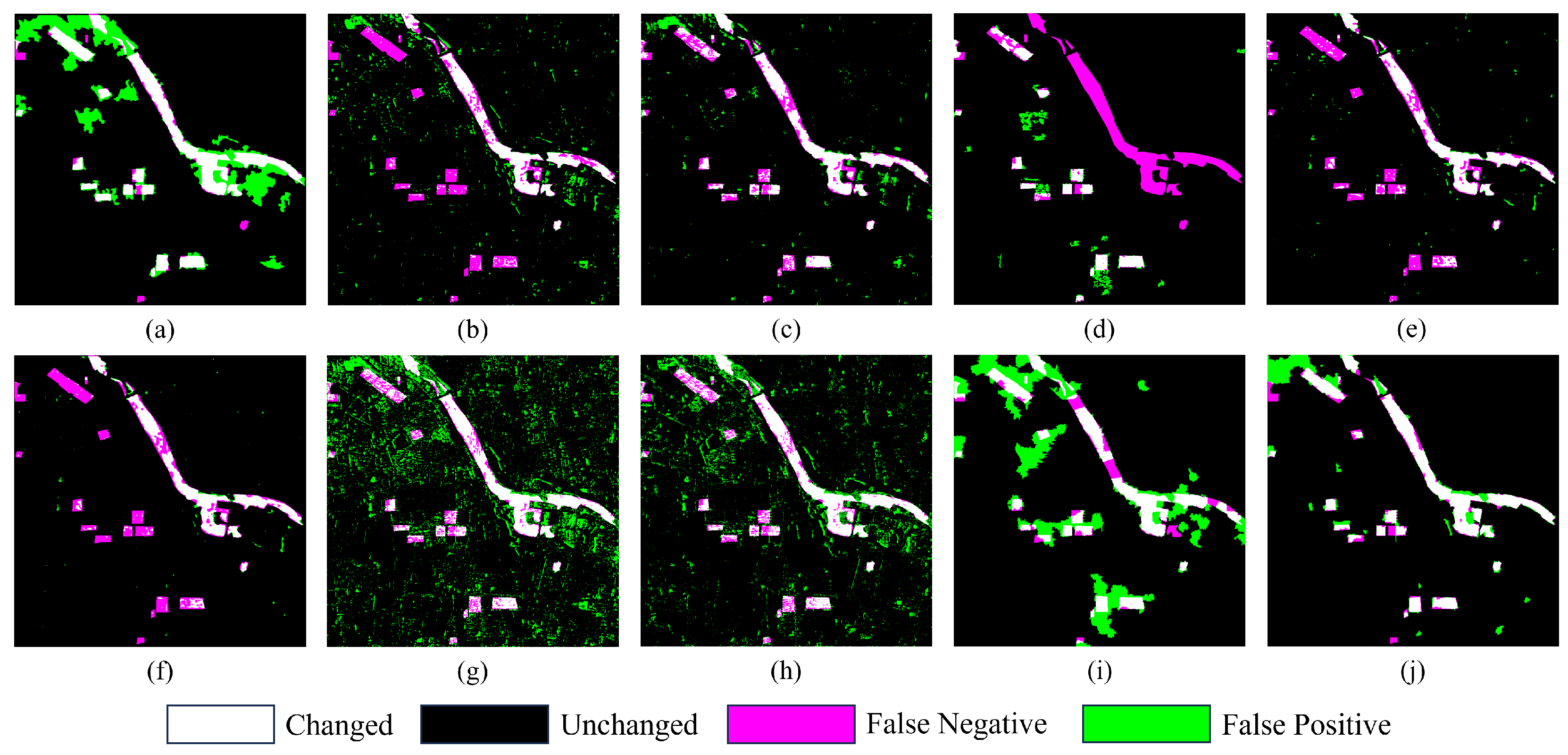
Figure 7 illustrates the change detection results of different methods on Dataset I. It can be observed that, compared to NLSW and HHG, SBMRF effectively eliminates pepper-like noise and captures most of the change areas. However, it also produces a significant number of false detections. NLSW and HHG effectively detect changes in water areas, but they fail to identify changes in building regions exhibiting high scattering, likely due to the nonlinear suppression inherent in ratio-based detectors. The LANTNet and SAFNet methods also miss many building regions, whereas the confusion maps produced by DDNet and CAMXier contain numerous false detected pixels, predominantly clustered around buildings. These observations indicate that deep networks struggle with robustness when processing change information in high-resolution building areas. In contrast, the proposed method [shown in Figure 7h] yields visually superior change maps. It detects most change areas while minimizing false alarms.
Table 1 presents the quantitative results on this dataset. The optimal and suboptimal results are highlighted in blue and red, respectively. From the table, it can be seen that the proposed method achieves optimal results in PCC, F1-score, and Kappa, which are 96.93%, 78.47%, and 76.83%, respectively, and sub-optimal values in RC (84.30%). HHG achieves sub-optimal results in F1 and Kappa, and our method compares to it with an improvement of 12.51% and 11.62%, which is attributed to the multi-scale modeling of GMRCS and the information fusion strategy of the FR module. These findings demonstrate the superiority of the proposed method over the comparison methods.

3.4.2. Change Detection Results on Dataset II

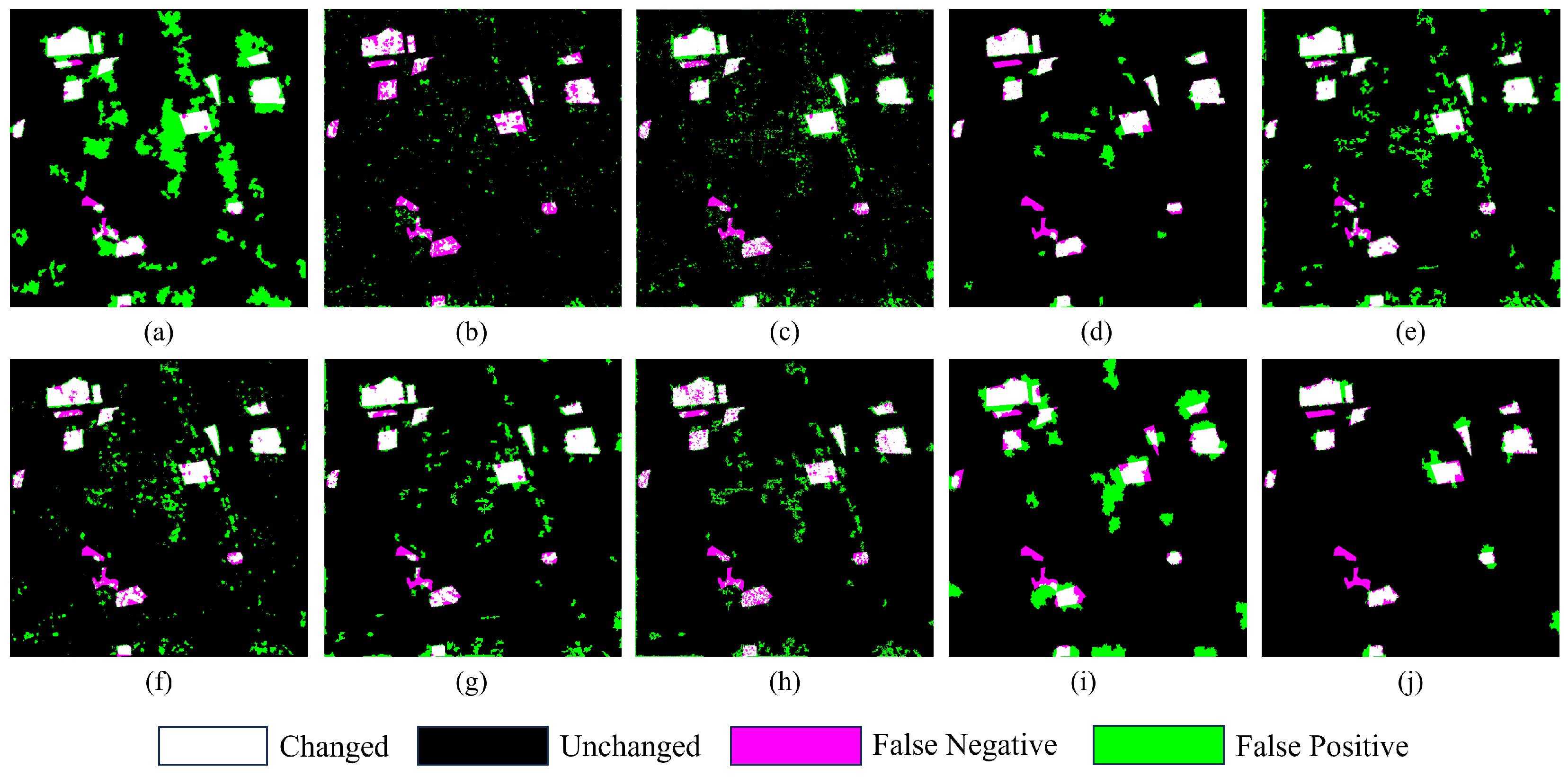
The changes occurring in Dataset II are mainly caused by submerged buildings, represented in the images as transitions from high to moderate scattering values. Confusion maps of various approaches are shown in Figure 8. It is noted that ratio-based methods face issues with nonlinear compression when handling such changes, potentially leading to detection failures. This inference can be confirmed by the results produced by NLSW [Figure 8b,c]. Additionally, Dataset II has slight misregistration errors on the left and bottom part of the co-registered bitemporal SAR images. Instead of removing this noise, we used it as a robustness test for the algorithm. In Figure 8c,d,f,g, elongated false alarm streaks can be seen, indicating that residual coregistration errors affect the performance of the comparison methods. By contrast, the proposed method [Figure 8h] effectively suppresses such distortion noise. Moreover, we found that deep learning methods tend to produce discrete patches, as shown in Figure 8d–g, likely due to their use of image patches for training and inference.
Table 1 reports the corresponding assessment results. From the results we know that on PCC, PRE, F1, and Kappa, HG obtains suboptimal and our method obtains optimal, indicating that the graph structure is effective in suppressing speckle noise. Notably, our method significantly outperforms HHG in all the metrics, with 0.65%, 9.62%, 5.45%, 7.55%, and 8.21% improvement, respectively. Interestingly, SBMRF achieved the highest RC (89.59%), yet it has the lowest PRE (29.68%). These findings clearly indicate that the proposed method significantly outperforms the comparison methods in detecting meaningful changes.

3.4.3. Change Detection Results on Dataset III

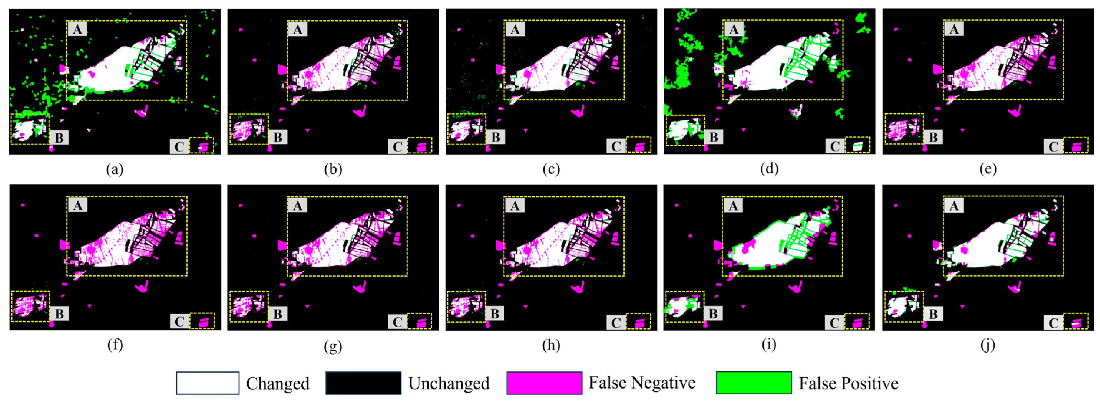
Dataset III contains extensive large-area changes as well as dense, small-area changes, posing a significant challenge to the precision of detection algorithms. As shown in Figure 9a, SBMRF produced the most false alarm regions. Other methods effectively suppressed speckle noise but missed a substantial amount of change information. The proposed method achieved a more balanced trade-off between False Point and Miss Point. Regarding the completeness of the detected changes, the comparison method failed to provide continuous change information, and only the proposed method maintains the integrity of the change regions, as shown Figure 9h. For boundary localization accuracy, the comparison methods produced numerous false detections along the edges of change regions, while the proposed method effectively determined the extent and boundaries of the changes. Table 1 shows the performance indicators. SBMRF and DDNet achieved the best results on two metrics, our method performed best on three critical metrics. The PCC, F1-score and Kappa of the proposed method achieved 3.39%, 13.20% and 16.29% higher than those of SBMRF, respectively, and 1.80%, 15.46%, and 17.03% higher than those of DDNet, respectively.
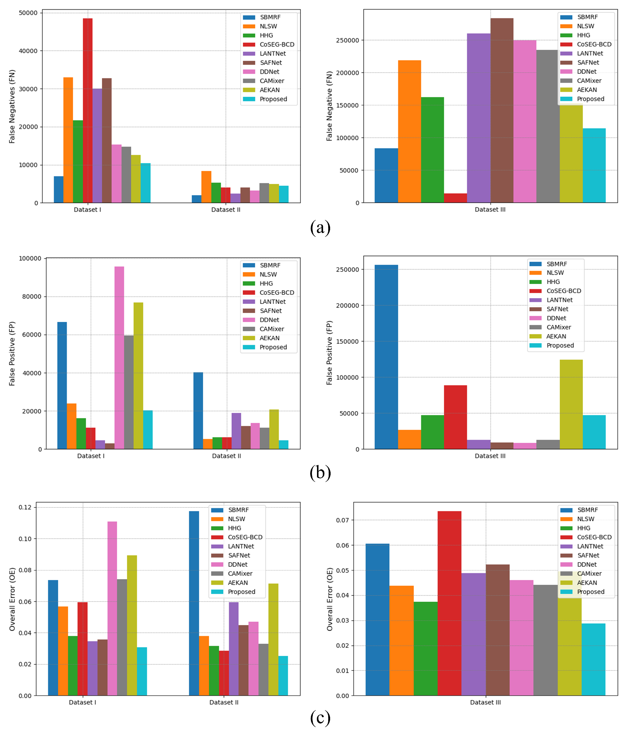
Figure 10 presents the FN, FP, and overall error (OE) statistics of different methods in histogram form. Although our method does not achieve the best performance on FN and FP across Datasets I, II, and III, it consistently yields the lowest OE. Notably, methods like NLSW and SBMRF usually produce diametrically opposed values of FN and FP: NLSW has low FP but high FN, while SBMRF shows the opposite trend. These results do not highlight the balance between FN and FP, whereas our method strikes a favorable compromise between FP and FN. This conclusion aligns with the visual and analytical findings in Figure 7, Figure 8 and Figure 9, further confirming the effectiveness and robustness of our method.

3.5. Ablation Study

3.5.1. Ablation Study for Graph-Based Strategy

The proposed GMRCS method offers the advantage of effectively balancing co-segmentation timeliness and accuracy. To evaluate its performance, we assess both the runtime and segmentation effectiveness of GMRCS on three datasets. Table 2 presents a comparison of the running times for GMRCS and the benchmark method MRJS across these datasets, where L represents the number of scales. From the results, it is evident that GMRCS achieves a shorter running time than MRJS. Notably, the current implementation of GMRCS has not been optimized by leveraging techniques such as multi-thread technology, block parallel, or GPU acceleration. With further optimization, we anticipate a significant improvement in the execution efficiency of GMRCS.
Figure 11 presents local slices of the segmentation results for both GMRCS and MRJS across the three datasets. It is evident that, by combining the graph-based greedy segmentation strategy with the proposed two-stage ranking strategy, GMRCS more effectively aligns with the edge structure of targets and extracts a more realistic geographic target. This characteristic contributes to reducing the holes and gaps and enhancing the completeness of change map, and thereby improve the accuracy of change detection.

3.5.2. Ablation Study for Two Stage Ranking

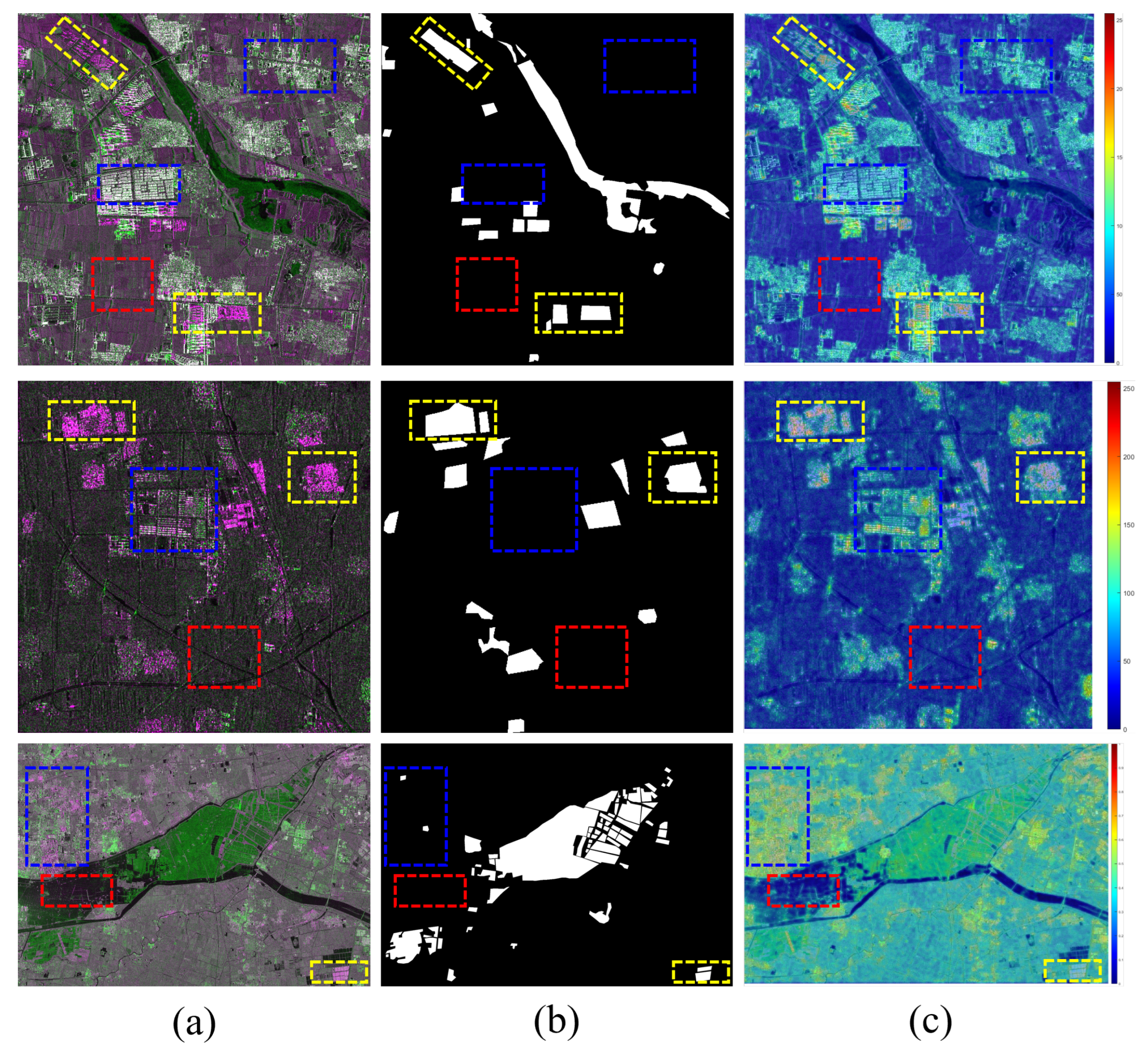
In this section, we evaluate the effectiveness of the Two-Stage Ranking (TSR) strategy in the GMRCS algorithm. Figure 12 visualizes the weights heat map of the edge set after TSR ranking. The first column shows the bi-temporal SAR pseudo-color image, which roughly distinguishes between changing and non-changing regions. The second column presents the ground truth, and the third column displays the weights heat map. Yellow, blue and red rectangular boxes highlight the changed regions, unchanged heterogeneous regions and unchanged homogeneous regions, respectively. Notably, the TSR strategy optimizes the merging order in co-segmentation by prioritizing the merging of non-changed homogeneous regions, thereby reducing edge noise and enhancing segmentation accuracy. As shown in Figure 12, the yellow and blue box regions have higher thermal values, while the red box regions have lower values. The weight of connecting edges increases with lower similarity between neighboring regions, leading to higher heat values. Consequently, in GMRCS, regions with lower heat values are merged first, while regions with higher heat values are merged later, demonstrating the effectiveness of the proposed two-stage ranking in improving co-segmentation.
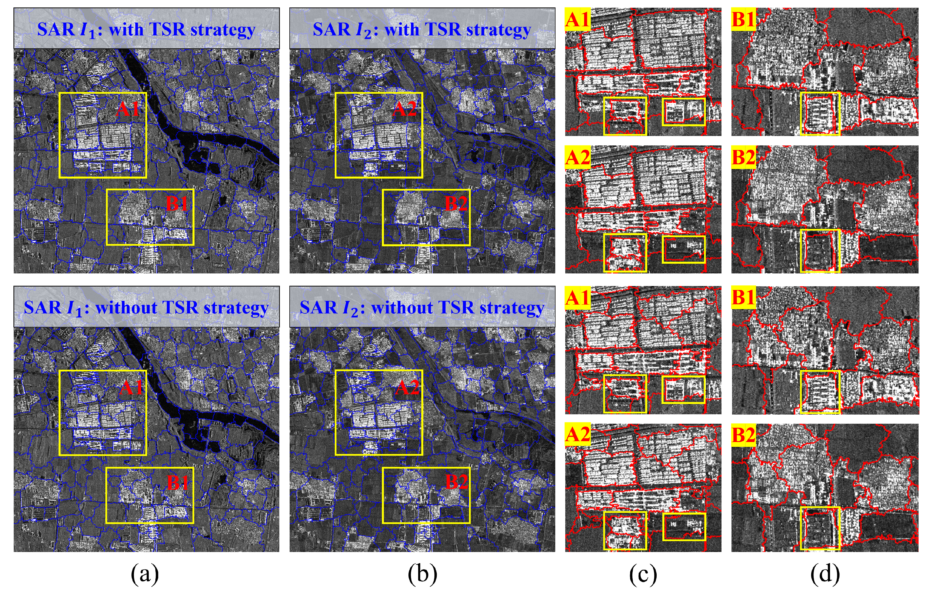
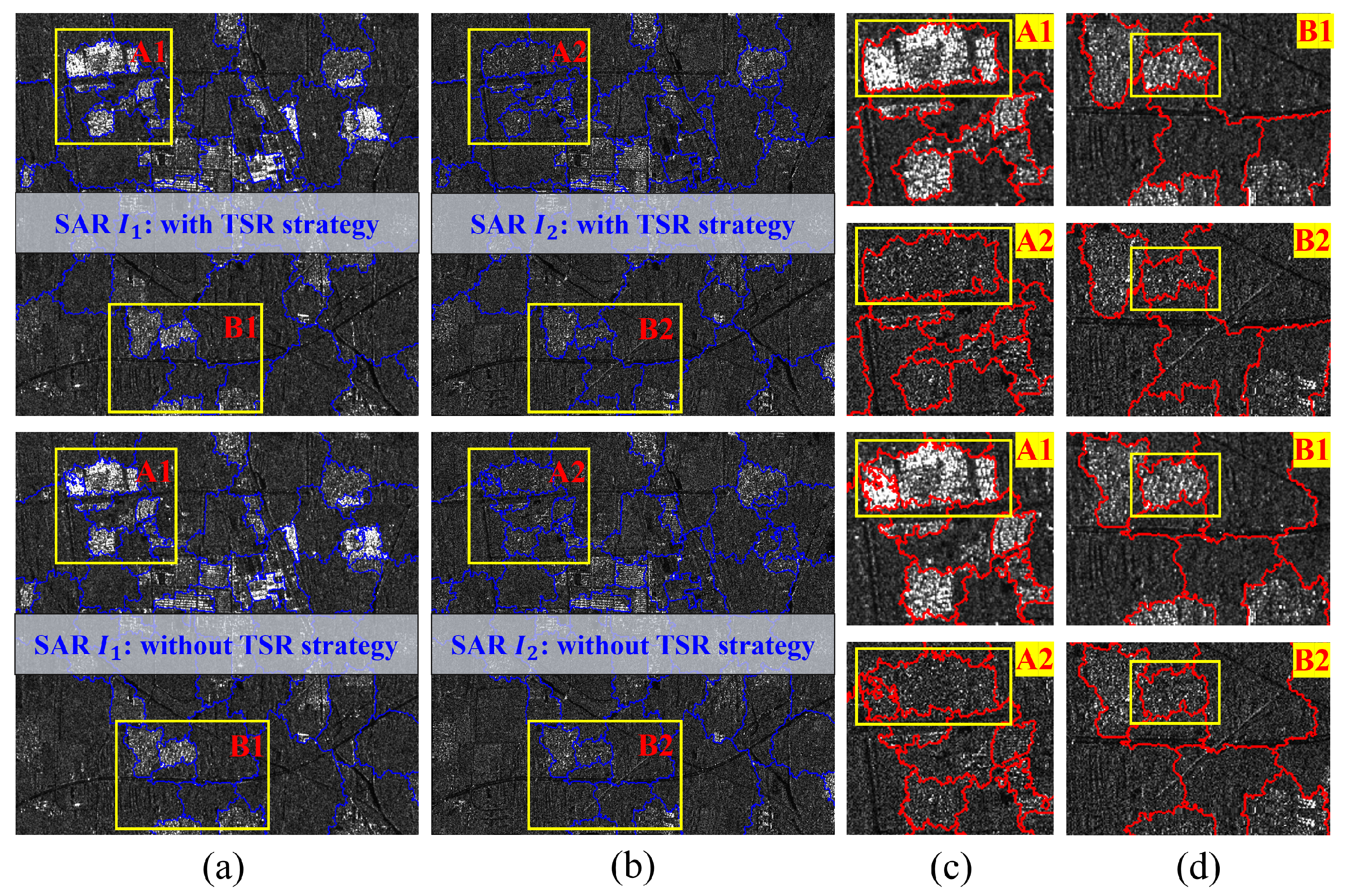
In this section, we use the segmentation results on Dataset I and Dataset II to verify the effectiveness of the proposed graph-based multi-resolution co-segmentation and proposed two-stage ranking (TSR) strategy. It worthy mentioning that there is currently no quantitative evaluation strategies for the segmentation results targeting change detection, hence our discussion is mainly focused on the qualitative analysis and comparisons. Figure 13 and Figure 14 display the segmentation results using proposed GMRCS on the two datasets, respectively, with the first row showing the results using the TSR strategy and the second row showing the results without the TSR strategy. Specifically, (c) and (d) of Figure 13 and Figure 14 show the enlarged segmentation results of slices A and B. From the yellow box, we can see that the change area is effectively segmented, indicating that collaborative interaction plays an important role in the segmentation process. If collaborative interactions are not implemented effectively, adjacent homogeneous regions will inevitably be merged. Therefore, through the joint analysis of the segmentation process, the change information on the bi-temporal SAR can be effectively retained without being merged into adjacent objects.
Further analysis of the overall segmentation results in Figure 13 and Figure 14, we can find that the joint segmentation with the TSR strategy is significantly better than the results without the strategy. For example, by observing the regions A and B in Figure 13c,d and Figure 14c,d, we find that the segmentation boundary is more accurate and the contour of the building area is more complete after adding TSR, while the results without TSR are over-segmented. It may lead to inaccurate measures of change differences, and in turn affects the detection integrity of change information.

3.5.3. Ablation Study for Fusion Refinement Module

In the proposed method, the Fusion Refinement (FR) module is primarily used to integrate change information across different segmentation scales, thereby reducing missed detections caused by erroneous merges and enhancing the preservation of small-scale change targets. Therefore, this section illustrates the effectiveness of the FR module through a case of incorrect merging.
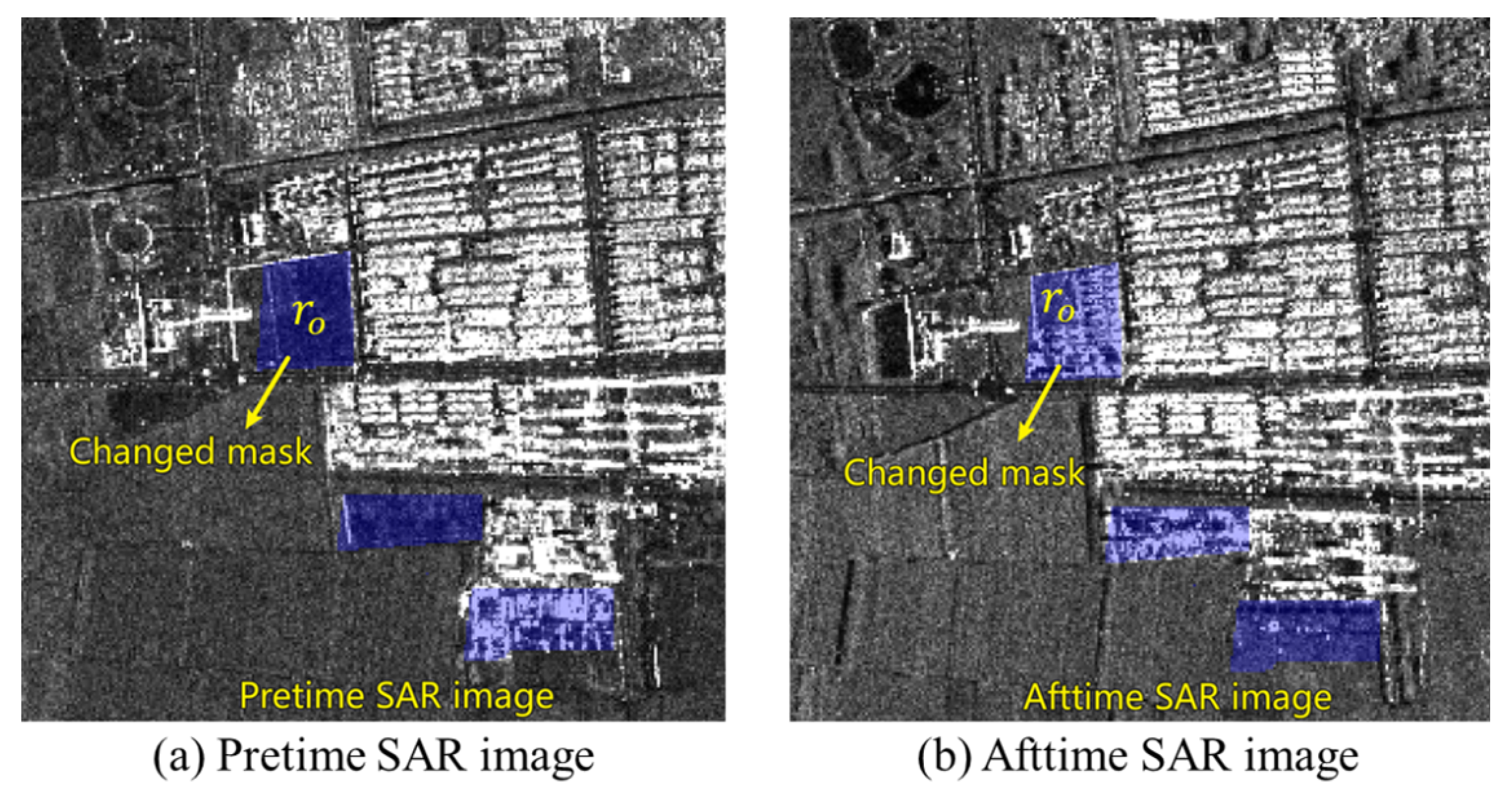
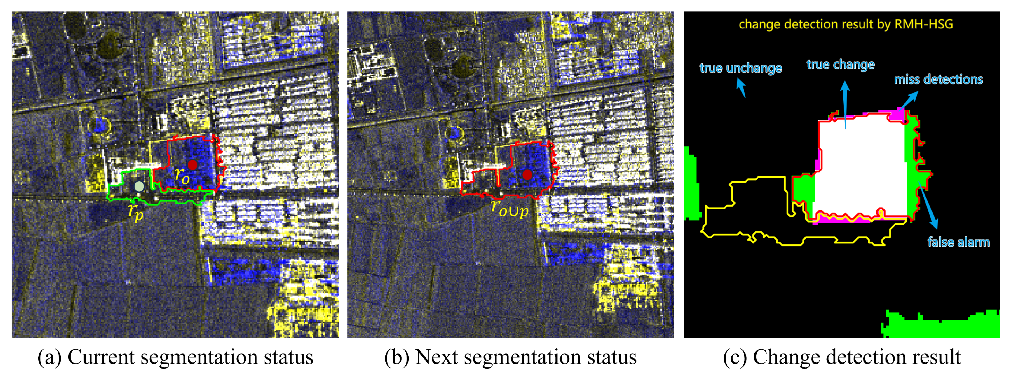
As shown in Figure 15, the overlay of bi-temporal SAR images and the ground truth highlights the changed region r o indicated by the yellow arrow as a representative example.
Figure 16 further illustrates instances where the proposed GMRCS method mistakenly merges regions during co-segmentation, where blue and yellow regions indicate the changes. Specifically, Figure 16a shows the current segmentation status, and Figure 16b shows the next segmentation status. It can be observed that when the current segmentation state progresses to the next one, the changed region r o and its adjacent unchanged region r p are erroneously merged into a larger superpixel r o p , resulting in partial omission of r o .
Despite these local merging errors, the proposed method incorporates a multi-scale fusion and refinement module (FR) in subsequent stages, which integrates change information across scales, providing overall robustness and tolerance to such errors. Figure 16c presents the confusion map of change detection results obtained by our method, showing that although there are minor omissions and false alarms around r o , the changed target is largely correctly identified. This demonstrates that the FR module effectively mitigates the impact of erroneous merging while preserving the structure of small-scale changed regions.

3.6. Key Parameter Analysis

We analyze three key parameters of the proposed method: the grid size r g r i d , the shape heterogeneity weight parameter ω s h a p e and the smoothness heterogeneity parameter ω s m o o t h of GMRCS. Figure 17 shows the performance curves for these parameters. From Figure 17a, we can observe that the kappa of the proposed method increases and then reaches stable as r g r i d increases. The best performance is achieved when r g r i d = 5 . Figure 17b,c hightlight the effect of GMRCS parameters on the change detection performance. Notably, ω s h a p e and ω s m o o t h have less impact on Dataset III but significantly impact datasets I and II. This may be attributed to the greater homogeneity of land cover in Dataset III. The segmentation parameters should typically be adjusted according to land cover types and background complexity of the data. When ω s h a p e is 0.7, the proposed algorithm performs best on datasets I and II. Similarly, when ω s m o o t h is 0.7, the RMF-HSG yields optimal results on Dataset II and obtains near-optimal results on Dataset I. Therefore, we recommend setting ω s h a p e = 0.7 , ω s m o o t h = 0.7 for GMRCS and r g r i d = 5 to ensure balanced performance across various datasets.

3.7. Comparison of GMRCS and SAM for Change Detection

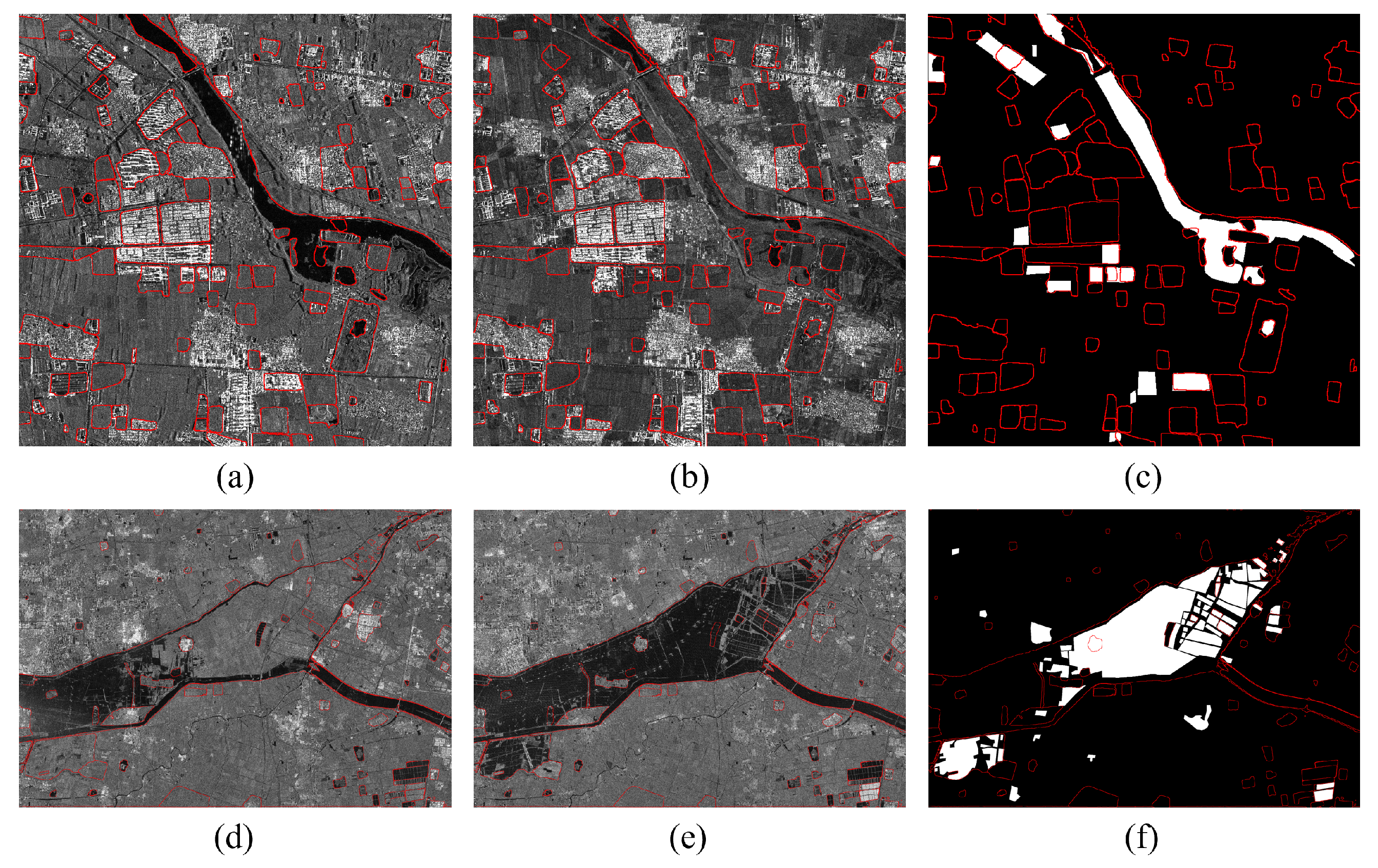
The vision fundamental model represents an important recent development in the field of computer vision. Among them, SAM (Segment Anything Model) [54] is the first foundation model for prompt-based image segmentation, which has strong zero-shot generalization ability and can adapt to unknown objects and data distribution. At present, SAM has been preliminarily applied to optical remote sensing images, and can generate segmentation masks for different targets. However, in the SAR images change detection task, SAM has not yet reached expectations. In this study, we applied SAM to segment Dataset I and Dataset II, and we analyze its limitations in the SAR change detection. Specifically, SAR is used to segment the pseudo-color image formed by superimposing the bi-temporal images on the channel. And then, the segmentation mask is superimposed to the bi-temporal SAR images and ground truth. Figure 18 displays this process. The results show that SAM can effectively divide the image into a background area and several compact foreground targets. For example, in Figure 18a–c, the SAM successfully extracts salient targets, such as building areas. However, SAM is deficient in extracting all areas that are subject to change. In Figure 18d,e, many of the changed targets are incorrectly segmented into background category, which leads to serious missed detections. In addition, the segmentation precision of the SAM method is insufficient, and many unchanged targets and the changed targets are segmented into the same mask, which leads to false alarms. Therefore, the adaptability of SAM in SAR image change detection still needs to be further studied to improve its segmentation and detection performance in complex scenes.

4. Discussion

(1)
Algorithm Effectiveness Analysis: The proposed RMF-HSG method is centered on multi-level spatial structural associations and aims to address two key issues in SAR change detection: high false alarms caused by speckle noise and inconsistent boundaries or poor internal connectivity in pixel-level methods. Its effectiveness is mainly reflected in three aspects. First, the GMRCS module introduces spatiotemporal constraints into multi-temporal co-segmentation, ensuring precise boundaries and regional integrity of change areas across multiple scales. Second, the HSG module employs a pixel–region–structure hierarchical graph consistency measure, effectively suppressing the influence of speckle noise on change intensity estimation. Finally, the FR module fuses multi-scale change information to enhance the detection of small-scale change targets. The three modules work collaboratively to improve both accuracy and stability of change detection. As shown in the experimental results (Figure 7, Figure 8 and Figure 9), the proposed method produces change maps with clear boundaries, low false alarms, and coherent change regions, confirming its effectiveness.
(2)
Comparison with Existing Methods: Existing SAR change detection methods can be broadly categorized into hand-crafted and deep learning-based approaches. The proposed method belongs to the former category. In the experiments, we compared the proposed algorithm with several representative methods, and both visual and quantitative results demonstrated its superiority. Compared with hand-crafted methods (SBMRF, NLSW, HHG, CoSEG-BCD), the proposed method exploits the stability of spatial structural associations to achieve stronger noise suppression. Moreover, by introducing spatiotemporal constraints (the TSR strategy) into multi-temporal co-segmentation, it achieves more precise boundary localization at the object level. In contrast, deep learning-based CD methods (LANTNet, DDNet, CAMixer) often suffer from limited training data quality and quantity, making it difficult to handle complex change scenarios. Furthermore, their small patch-based training leads to fragmented detection results, reducing precision and usability. In addition, DLCD methods require pseudo-sample extraction, network training, and inference, resulting in longer processing time. As shown in Table 3, the proposed method runs significantly faster than three representative DLCD methods.
(3)
Algorithm Generalization Analysis: The generalization capability of the algorithm is mainly reflected in its adaptability to different scenarios and its stability with respect to parameter settings. The proposed method is not tailored to any specific scene and is theoretically applicable to various surface types. From a modular perspective, GMRCS guides segmentation by assessing feature consistency among adjacent regions and considering temporal changes, but in highly heterogeneous areas such as dense urban scenes, layover, double bounce, and shadows may cause mis-segmentation, which can further affect the structural relationship description in HSG. Fortunately, the spectral and shape weighting parameters w spectral and w shape in GMRCS can mitigate this issue to some extent. The parameter sensitivity analysis (Section 3.6) shows that the algorithm is relatively stable with respect to key parameters; moreover, when the geometric feature weight is higher ( w shape > w spectral ), the detection performance improves. This indicates that emphasizing geometric feature modeling in SAR imagery is more beneficial for change detection.
(4)
Algorithm Limitations: The algorithm assumes a high-precision registration between multi-temporal images; thus, its performance may degrade under severe geometric distortions or large viewing angle differences. For example, in ultra-high-resolution SAR images of dense urban areas, the algorithm may fail to precisely capture change boundaries. Although the proposed method is more efficient and produces more coherent results than DLCD methods, its computational efficiency is slightly lower than pixel-level approaches due to the multi-temporal segmentation process. Furthermore, its performance across different scenarios (e.g., urban, vegetation, coastal, mountainous) remains sensitive to parameter settings, requiring manual adjustment for optimal results.
(5)
Future Research: Future work will focus on adapting the algorithm to different scenarios. Specifically, GMRCS will be enhanced to automatically adjust segmentation thresholds based on scene characteristics, and HSG will be extended to construct spatial associations at the semantic feature rather than merely the low feature level. In addition, scene-specific SAR scattering priors will be incorporated to further improve the detection performance of the algorithm in complex environments.

5. Conclusions

This paper proposes an object-level change detection method for high-resolution SAR images, which effectively extracts change information through multi-scale segmentation and multi-level change difference fusion model. The proposed change detection method consists of two stages: First, in the segmentation stage, a graph-driven multi-resolution co-segmentation framework is designed, incorporating an effective two stage ranking strategy to ensure that primitives with high spatiotemporal consistency are prioritized during cooperative merging, resulting in high-quality multi-level segmentation masks. Second, in the multi-level difference fusion stage, an improved region-based structural graph detector is used to extract change intensity from bi-temporal SAR images at different scales. And a designed fusion model is applied to integrate the multi-scale changes, ensuring effective detection of changed targets with various scale properties. Comparisons with several state-of-the-art algorithms demonstrate that the proposed method achieves superior performance in change detection accuracy and change information completeness, showing significant potential for engineering applications.

Author Contributions

Conceptualization, J.Z.; methodology, J.Z.; software, J.Z.; validation, J.Z.; formal analysis, M.Y.; investigation, J.Z.; resources, J.Z.; data curation, J.Z.; writing—original draft preparation, J.Z.; writing—review and editing, M.Y.; visualization, J.Z.; supervision, F.W., G.Z., N.J., Y.X. and H.Y. All authors have read and agreed to the published version of the manuscript.

Funding

This research received no external funding.

Data Availability Statement

No new data were created in this manuscript.

Conflicts of Interest

The authors declare no conflict of interest.

References

  1. Zhu, J.; Zhou, G.; Wang, F.; Liu, R.; Xiang, Y.; Wang, W.; You, H. Multi-temporal sar images change detection considering ambiguous co-registration errors: A unified framework. IEEE Geosci. Remote Sens. Lett. 2024, 21, 4019405. [Google Scholar] [CrossRef]
  2. Quan, S.; Xiong, B.; Xiang, D.; Zhao, L.; Zhang, S.; Kuang, G. Eigenvalue-based urban area extraction using polarimetric sar data. IEEE J. Sel. Top. Appl. Earth Obs. Remote Sens. 2018, 11, 458–471. [Google Scholar] [CrossRef]
  3. Wang, B.; Zhao, C.; Zhang, Q.; Lu, Z.; Pepe, A. Long-term continuously updated deformation time series from multisensor insar in xi’an, china from 2007 to 2021. IEEE J. Sel. Top. Appl. Earth Obs. Remote Sens. 2021, 14, 7297–7309. [Google Scholar] [CrossRef]
  4. Zou, B.; Li, W.; Zhang, L. Built-up area extraction using high-resolution sar images based on spectral reconfiguration. IEEE Geosci. Remote Sens. Lett. 2020, 18, 1391–1395. [Google Scholar] [CrossRef]
  5. Adeli, S.; Salehi, B.; Mahdianpari, M.; Quackenbush, L.J.; Brisco, B.; Tamiminia, H.; Shaw, S. Wetland monitoring using sar data: A meta-analysis and comprehensive review. Remote Sens. 2020, 12, 2190. [Google Scholar] [CrossRef]
  6. Tsokas, A.; Rysz, M.; Pardalos, P.M.; Dipple, K. Sar data applications in earth observation: An overview. Expert Syst. Appl. 2022, 205, 117342. [Google Scholar] [CrossRef]
  7. Brunner, D.; Lemoine, G.; Bruzzone, L. Earthquake damage assessment of buildings using vhr optical and sar imagery. IEEE Trans. Geosci. Remote Sens. 2010, 48, 2403–2420. [Google Scholar] [CrossRef]
  8. AlAli, Z.T.; Alabady, S.A. A survey of disaster management and sar operations using sensors and supporting techniques. Int. J. Disaster Risk Reduct. 2022, 82, 103295. [Google Scholar] [CrossRef]
  9. Sun, Z.; Dai, M.; Leng, X.; Lei, Y.; Xiong, B.; Ji, K.; Kuang, G. An anchor-free detection method for ship targets in high-resolution sar images. IEEE J. Sel. Top. Appl. Earth Obs. Remote Sens. 2021, 14, 7799–7816. [Google Scholar] [CrossRef]
  10. Zhao, Y.; Zhao, L.; Xiong, B.; Kuang, G. Attention receptive pyramid network for ship detection in sar images. IEEE J. Sel. Top. Appl. Earth Obs. Remote Sens. 2020, 13, 2738–2756. [Google Scholar] [CrossRef]
  11. Xiang, Y.; Teng, F.; Wang, L.; Jiao, N.; Wang, F.; You, H. Orthorectification of high-resolution sar images in island regions based on fast multimodal registration. J. Radars 2024, 13, 1–19. [Google Scholar]
  12. Xiang, Y.; Jiao, N.; Liu, R.; Wang, F.; You, H.; Qiu, X.; Fu, K. A geometry-aware registration algorithm for multiview high-resolution sar images. IEEE Trans. Geosci. Remote Sens. 2022, 60, 5234818. [Google Scholar] [CrossRef]
  13. Xiang, Y.; Jiang, L.; Wang, F.; You, H.; Qiu, X.; Fu, K. Detector-free feature matching for optical and sar images based on a two-step strategy. IEEE Trans. Geosci. Remote Sens. 2024, 62, 5214216. [Google Scholar] [CrossRef]
  14. Jiao, N.; Wang, F.; Hu, Y.; Xiang, Y.; Liu, R.; You, H. Sar true digital ortho maps production for target geometric structure preservation. IEEE J. Sel. Top. Appl. Earth Obs. Remote Sens. 2023, 16, 10279–10286. [Google Scholar] [CrossRef]
  15. Gong, M.; Cao, Y.; Wu, Q. A neighborhood-based ratio approach for change detection in sar images. IEEE Geosci. Remote Sens. Lett. 2011, 9, 307–311. [Google Scholar] [CrossRef]
  16. Zhuang, H.; Tan, Z.; Deng, K.; Yao, G. Adaptive generalized likelihood ratio test for change detection in sar images. IEEE Geosci. Remote Sens. Lett. 2019, 17, 416–420. [Google Scholar] [CrossRef]
  17. Saha, S.; Bovolo, F.; Bruzzone, L. Building change detection in vhr sar images via unsupervised deep transcoding. IEEE Trans. Geosci. Remote Sens. 2020, 59, 1917–1929. [Google Scholar] [CrossRef]
  18. Pirrone, D.; De, S.; Bhattacharya, A.; Bruzzone, L.; Bovolo, F. Unsupervised change detection in built-up areas by multi-temporal polarimetric sar images. In Proceedings of the 2017 IEEE International Geoscience and Remote Sensing Symposium (IGARSS), Fort Worth, TX, USA, 23–28 July 2017; pp. 4554–4557. [Google Scholar]
  19. Wang, J.; Yang, X.; Jia, L. Pointwise sar image change detection based on stereograph model with multiple-span neighbourhood information. Int. J. Remote Sens. 2019, 40, 31–50. [Google Scholar] [CrossRef]
  20. Wang, J.; Zeng, F.; Niu, S.; Zheng, J.; Jiang, X. Sar image change detection via heterogeneous graph with multi-order and multi-level connections. IEEE J. Sel. Top. Appl. Earth Obs. Remote Sens. 2024, 17, 11386–11401. [Google Scholar] [CrossRef]
  21. Zhu, J.; Wang, F.; You, H. Unsupervised sar image change detection based on structural consistency and cfar threshold estimation. Remote Sens. 2023, 15, 1422. [Google Scholar] [CrossRef]
  22. Fu, B.; Wang, Y.; Campbell, A.; Li, Y.; Zhang, B.; Yin, S.; Xing, Z.; Jin, X. Comparison of object-based and pixel-based random forest algorithm for wetland vegetation mapping using high spatial resolution gf-1 and sar data. Ecol. Indic. 2017, 73, 105–117. [Google Scholar] [CrossRef]
  23. Wan, L.; Zhang, T.; You, H. Object-based multiscale method for sar image change detection. J. Appl. Remote Sens. 2018, 12, 025004. [Google Scholar] [CrossRef]
  24. Wan, L.; Zhang, T.; You, H. An object-based method based on a novel statistical distance for sar image change detection. In Proceedings of the 2018 IEEE 3rd International Conference on Signal and Image Processing (ICSIP), Shenzhen, China, 13–15 July 2018; pp. 172–176. [Google Scholar]
  25. Zhu, J.; Wang, F.; You, H. Segmentation-based vhr sar images built-up area change detection: A coarse-to-fine approach. J. Appl. Remote Sens. 2024, 18, 016503. [Google Scholar] [CrossRef]
  26. Cheng, G.; Huang, Y.; Li, X.; Lyu, S.; Xu, Z.; Zhao, H.; Zhao, Q.; Xiang, S. Change detection methods for remote sensing in the last decade: A comprehensive review. Remote Sens. 2024, 16, 2355. [Google Scholar] [CrossRef]
  27. Xue, W.; Ai, J.; Zhu, Y.; Chen, J.; Zhuang, S. Ais-fcanet: Long-term ais data assisted frequency-spatial contextual awareness network for salient ship detection in sar imagery. IEEE Trans. Aerosp. Electron. Syst. 2025, 61, 15166–15171. [Google Scholar] [CrossRef]
  28. Wang, R.; Chen, J.-W.; Wang, Y.; Jiao, L.; Wang, M. Sar image change detection via spatial metric learning with an improved mahalanobis distance. IEEE Geosci. Remote Sens. Lett. 2019, 17, 77–81. [Google Scholar] [CrossRef]
  29. Gao, F.; Dong, J.; Li, B.; Xu, Q. Automatic change detection in synthetic aperture radar images based on pcanet. IEEE Geosci. Remote Sens. Lett. 2016, 13, 1792–1796. [Google Scholar] [CrossRef]
  30. Gao, F.; Wang, X.; Gao, Y.; Dong, J.; Wang, S. Sea ice change detection in sar images based on convolutional-wavelet neural networks. IEEE Geosci. Remote Sens. Lett. 2019, 16, 1240–1244. [Google Scholar] [CrossRef]
  31. Zhang, X.; Su, H.; Zhang, C.; Gu, X.; Tan, X.; Atkinson, P.M. Robust unsupervised small area change detection from sar imagery using deep learning. ISPRS J. Photogramm. Remote Sens. 2021, 173, 79–94. [Google Scholar] [CrossRef]
  32. Qu, X.; Gao, F.; Dong, J.; Du, Q.; Li, H.-C. Change detection in synthetic aperture radar images using a dual-domain network. IEEE Geosci. Remote Sens. Lett. 2022, 19, 4013405. [Google Scholar] [CrossRef]
  33. Zhang, H.; Lin, Z.; Gao, F.; Dong, J.; Du, Q.; Li, H.-C. Convolution and attention mixer for synthetic aperture radar image change detection. IEEE Geosci. Remote Sens. Lett. 2023, 20, 4012105. [Google Scholar] [CrossRef]
  34. Xie, J.; Gao, F.; Zhou, X.; Dong, J. Wavelet-based bi-dimensional aggregation network for sar image change detection. IEEE Geosci. Remote Sens. Lett. 2024, 21, 4013705. [Google Scholar] [CrossRef]
  35. Zhang, X.; Liu, G.; Zhang, C.; Atkinson, P.M.; Tan, X.; Jian, X.; Zhou, X.; Li, Y. Two-phase object-based deep learning for multi-temporal sar image change detection. Remote Sens. 2020, 12, 548. [Google Scholar] [CrossRef]
  36. Ji, L.; Zhao, J.; Zhao, Z. A novel end-to-end unsupervised change detection method with self-adaptive superpixel segmentation for sar images. Remote Sens. 2023, 15, 1724. [Google Scholar] [CrossRef]
  37. Ai, J.; Mao, Y.; Luo, Q.; Jia, L.; Xing, M. Sar target classification using the multikernel-size feature fusion-based convolutional neural network. IEEE Trans. Geosci. Remote Sens. 2021, 60, 5214313. [Google Scholar] [CrossRef]
  38. Ning, X.; Zhang, H.; Zhang, R.; Huang, X. Multi-stage progressive change detection on high resolution remote sensing imagery. ISPRS J. Photogramm. Remote Sens. 2024, 207, 231–244. [Google Scholar] [CrossRef]
  39. Zhao, C.; Ma, L.; Wang, L.; Ohtsuki, T.; Mathiopoulos, P.T.; Wang, Y. Sar image change detection in spatial-frequency domain based on attention mechanism and gated linear unit. IEEE Geosci. Remote Sens. Lett. 2023, 20, 4002205. [Google Scholar] [CrossRef]
  40. Yi, W.; Wang, S.; Ji, N.; Wang, C.; Xiao, Y.; Song, X. Sar image change detection based on gabor wavelets and convolutional wavelet neural networks. Multimed. Tools Appl. 2023, 82, 30895–30908. [Google Scholar] [CrossRef]
  41. Li, T.; Liang, Z.; Zhao, S.; Gong, J.; Shen, J. Self-learning with rectification strategy for human parsing. In Proceedings of the 2020 IEEE/CVF Conference on Computer Vision and Pattern Recognition (CVPR), Seattle, WA, USA, 13–19 June 2020; pp. 9260–9269. [Google Scholar] [CrossRef]
  42. Peng, Y.; Cui, B.; Yin, H.; Zhang, Y.; Du, P. Automatic sar change detection based on visual saliency and multi-hierarchical fuzzy clustering. IEEE J. Sel. Top. Appl. Earth Obs. Remote Sens. 2022, 15, 7755–7769. [Google Scholar] [CrossRef]
  43. Meng, D.; Gao, F.; Dong, J.; Du, Q.; Li, H.-C. Synthetic aperture radar image change detection via layer attention-based noise-tolerant network. IEEE Geosci. Remote Sens. Lett. 2022, 19, 4026505. [Google Scholar] [CrossRef]
  44. Fang, S.; Qi, C.; Yang, S.; Li, Z.; Wang, W.; Wang, Y. Unsupervised sar change detection using two-stage pseudo labels refining framework. IEEE Geosci. Remote Sens. Lett. 2024, 21, 4005405. [Google Scholar] [CrossRef]
  45. Zhang, H.; Lin, M.; Yang, G.; Zhang, L. Escnet: An end-to-end superpixel-enhanced change detection network for very-high-resolution remote sensing images. IEEE Trans. Neural Netw. Learn. Syst. 2021, 34, 28–42. [Google Scholar] [CrossRef]
  46. Gong, M.; Zhan, T.; Zhang, P.; Miao, Q. Superpixel-based difference representation learning for change detection in multispectral remote sensing images. IEEE Trans. Geosci. Remote Sens. 2017, 55, 2658–2673. [Google Scholar] [CrossRef]
  47. Duan, Y.; Sun, K.; Li, W.; Wei, J.; Gao, S.; Tan, Y.; Zhou, W.; Liu, J.; Liu, J. Wcmu-net: An effective method for reducing the impact of speckle noise in sar image change detection. IEEE J. Sel. Top. Appl. Earth Obs. Remote Sens. 2024, 18, 2880–2892. [Google Scholar] [CrossRef]
  48. Zhang, W.; Xiang, D.; Su, Y. Fast multiscale superpixel segmentation for sar imagery. IEEE Geosci. Remote Sens. Lett. 2020, 19, 4001805. [Google Scholar] [CrossRef]
  49. Wang, J.; Zhao, T.; Jiang, X.; Lan, K. A hierarchical heterogeneous graph for unsupervised sar image change detection. IEEE Geosci. Remote Sens. Lett. 2022, 19, 4516605. [Google Scholar] [CrossRef]
  50. Hao, M.; Zhou, M.; Jin, J.; Shi, W. An advanced superpixel-based markov random field model for unsupervised change detection. IEEE Geosci. Remote Sens. Lett. 2019, 17, 1401–1405. [Google Scholar] [CrossRef]
  51. Zhang, K.; Fu, X.; Lv, X.; Yuan, J. Unsupervised multitemporal building change detection framework based on cosegmentation using time-series sar. Remote Sens. 2021, 13, 471. [Google Scholar] [CrossRef]
  52. Gao, Y.; Gao, F.; Dong, J.; Du, Q.; Li, H.-C. Synthetic aperture radar image change detection via siamese adaptive fusion network. IEEE J. Sel. Top. Appl. Earth Obs. Remote Sens. 2021, 14, 10748–10760. [Google Scholar] [CrossRef]
  53. Liu, T.; Xu, J.; Lei, T.; Wang, Y.; Du, X.; Zhang, W.; Lv, Z.; Gong, M. Aekan: Exploring superpixel-based autoencoder kolmogorov-arnold network for unsupervised multimodal change detection. IEEE Trans. Geosci. Remote Sens. 2025, 63, 5601114. [Google Scholar] [CrossRef]
  54. Kirillov, A.; Mintun, E.; Ravi, N.; Mao, H.; Rolland, C.; Gustafson, L.; Xiao, T.; Whitehead, S.; Berg, A.C.; Lo, W.-Y.; et al. Segment anything. In Proceedings of the IEEE/CVF International Conference on Computer Vision, Paris, France, 2–6 October 2023; pp. 4015–4026. [Google Scholar]
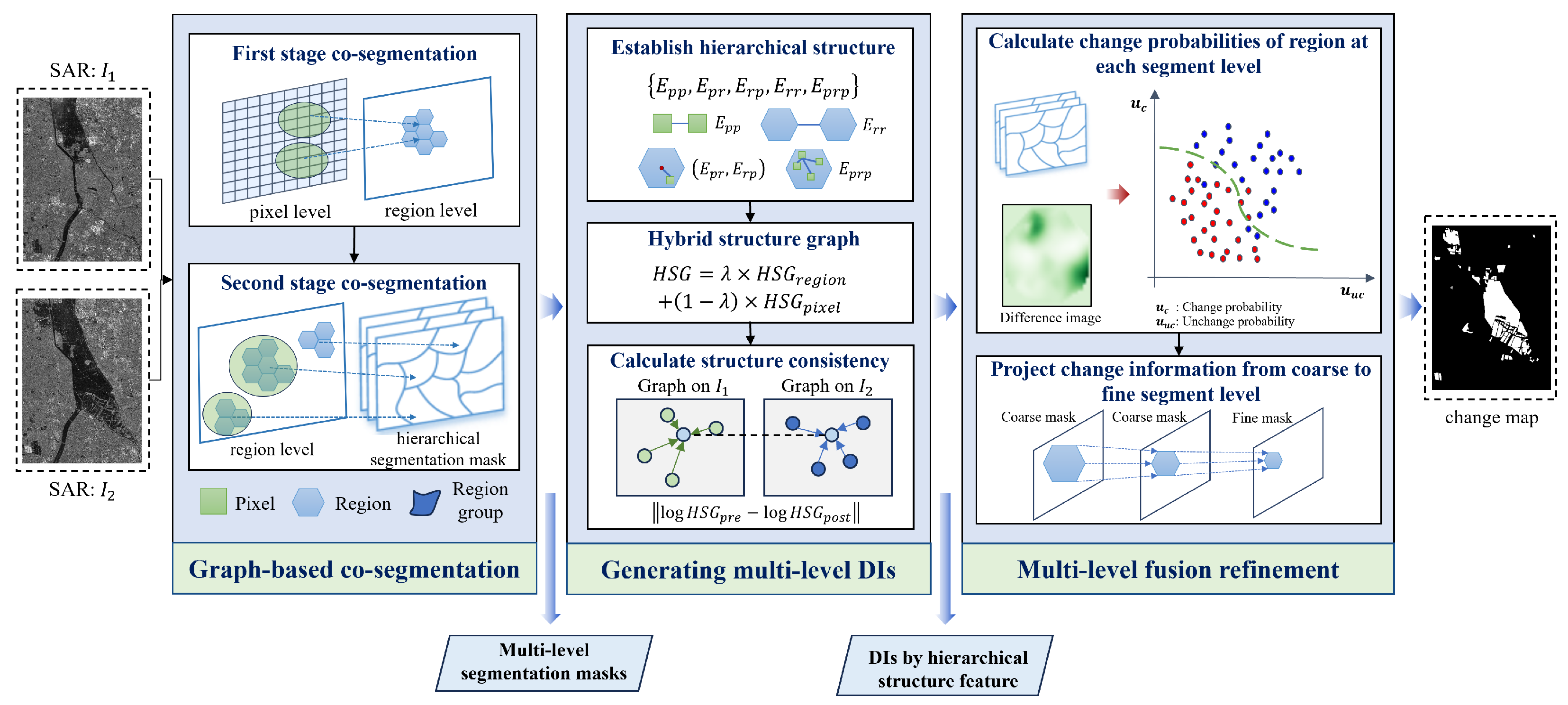
Figure 1. The flowchart of the proposed VHR SAR image change detection method based on graph-based multi-resolution co-segmentation and structure features fusion.
Remotesensing 17 03736 g001
Figure 2. The co-segmentation illustration of bi-temporal SAR images.
Remotesensing 17 03736 g002
Figure 3. Illustration of the second-stage ranking strategy. (a) pretime SAR image; (b) posttime SAR image; (c) ground truth. #1, #2, #3 denote three cases of edge pairs, denoted as ( e # 1 , p r e , e # 1 , p o s t ) , ( e # 2 , p r e , e # 2 , p o s t ) , and ( e # 3 , p r e , e # 3 , p o s t ) .
Remotesensing 17 03736 g003
Figure 4. The flowchart of proposed graph-based multi-resolution co-segmentation. It contains the first segmentation and second segmentation stage.
Remotesensing 17 03736 g004
Figure 5. Illustration of regional key pixel selection. (a) KNN-based regional key pixel extraction. (b) Region key point extraction based on grid sampling. In (a,b) blue lines indicate the regional boundaries in the segmentation results. In (a), green and blue denote two center pixels, and pink and yellow are their corresponding key pixels by KNN, respectively.
Remotesensing 17 03736 g005
Figure 6. Three SAR change detection datasets used in experiments. From left to right are Dataset I, Dataset II, and Dataset III. From top to bottom are the pre-event SAR image, post-event SAR image, and ground truth.
Remotesensing 17 03736 g006
Figure 7. Change detection results using different methods on Dataset I. (a) SBMRF; (b) NLSW; (c) HHG; (d) CoSEG-BCD; (e) LANTNet; (f) SAFNet; (g) DDNet; (h) CAMXier; (i) AEKAN; (j) Proposed RMF-HSG. In the confusion change map, white: TP; Black: TN; Magenta: FN; Green: FP.
Remotesensing 17 03736 g007
Figure 8. Change detection results using different methods on Dataset II. (a) SBMRF; (b) NLSW; (c) HHG; (d) CoSEG-BCD; (e) LANTNet; (f) SAFNet; (g) DDNet; (h) CAMXier; (i) AEKAN; (j) Proposed RMF-HSG. In the confusion change map, white: TP; Black: TN; Magenta: FN; Green: FP.
Remotesensing 17 03736 g008
Figure 9. Change detection results using different methods on Dataset III. (a) SBMRF; (b) NLSW; (c) HHG; (d) CoSEG-BCD; (e) LANTNet; (f) SAFNet; (g) DDNet; (h) CAMXier; (i) AEKAN; (j) Proposed RMF-HSG. In the confusion change map, white: TP; Black: TN; Magenta: FN; Green: FP.
Remotesensing 17 03736 g009
Figure 10. Comparison of three quantitative evaluation indices on Dataset I/II/III. (a) FNs of different methods. (b) FPs of different methods. (c) OE of different methods.
Remotesensing 17 03736 g010
Figure 11. Local slices of GMRCS and MRJS segmentation results on the three datasets. The first line of (ae) shows the segmentation results of the proposed GMRCS and the second line of (ae) shows the segmentation results of the comparison method MRJS.
Remotesensing 17 03736 g011
Figure 12. Weight visualization maps of edge sets after TSR ranking in the GMRCS method. (a) Bi-temporal pseudo-color images of the three datasets; (b) Groundtruth; (c) Heat maps of the weights after TSR ranking. Yellow boxes indicate changed regions, blue boxes indicate non-changed heterogeneous regions, and red boxes denote non-changed homogeneous regions. In the heat map, the lower the similarity of neighboring objects, the higher the connecting edge weight and the higher the heat value.
Remotesensing 17 03736 g012
Figure 13. Co-segmentation results with and without the TSR strategy and local zoomed slices on Dataset I. (a) Pretime segmentation results with and without the TSR strategy; (b) Posttime segmentation results with and without the TSR strategy; (c) Enlarged view of region A; (d) Enlarged view of region B.
Remotesensing 17 03736 g013
Figure 14. Co-segmentation results with and without the TSR strategy and local zoomed slices on Dataset II. (a) Pretime segmentation results with and without the TSR strategy; (b) Posttime segmentation results with and without the TSR strategy; (c) Local zoomed-in view of region A; (d) Local zoomed-in view of region B.
Remotesensing 17 03736 g014
Figure 15. The superimposed images between bi-temporal SAR images and ground truth.
Remotesensing 17 03736 g015
Figure 16. Illustration of local merging errors in the proposed GMRCS method and the robustness provided by the multi-scale Fusion–Refinement (FR) module. (a) Current segmentation status; (b) Next segmentation status; (c) Change detection result.
Remotesensing 17 03736 g016
Figure 17. The performance analysis of key parameters. (a) performance analysis of grid size r g r i d ; (b) performance analysis of GMRCS parameter ω s h a p e ; (c) performance analysis of GMRCS parameter ω s m o o t h .
Remotesensing 17 03736 g017
Figure 18. The segmentation results of the SAM segmentation model on Dataset I and Dataset III. The red lines represent the extracted foreground contours. (ac) The result of the segmentation boundary generated by SAM superimposed on Dataset I; (df) The result of the segmentation boundary generated by SAM superimposed on Dataset III.
Remotesensing 17 03736 g018
Table 1. The quantitative evaluation results of different algorithms on Dataset I/II/III. The optimal results are highlighted in blue, and suboptimal results are highlighted in red. Note: The ↑ indicates that the larger the value, the better the performance.
MethodsDataset IDataset IIDataset III
PCC(%) ↑PRE(%) ↑RC(%) ↑F1(%) ↑Kappa(%) ↑PCC(%) ↑PRE(%) ↑RC(%) ↑F1(%) ↑Kappa(%) ↑PCC(%) ↑PRE(%) ↑RC(%) ↑F1(%) ↑Kappa(%) ↑
SBMRF [50]92.6547.2189.5161.8158.1788.2629.6889.5944.5939.8293.9468.3586.9176.5273.10
NLSW [21]94.3258.4050.3454.0751.0696.2266.8156.1861.0459.0695.6294.0365.6577.3174.97
HHG [49]96.2273.5067.3770.3068.2996.8469.1672.4570.7769.1096.2690.9874.4781.9079.84
CoSEG-BCD [51]94.0461.7527.1037.6735.0497.1570.6078.6274.4072.8992.6562.0191.1673.8169.71
LANTNet [43]96.5388.6654.8667.7866.0694.0546.5587.0560.6757.7695.1296.7659.0973.3770.86
SAFNet [52]96.4491.9850.7965.4463.7395.5255.2879.0965.0862.7694.7897.4955.4770.7168.08
DDNet [32]88.9034.8477.0147.9842.8495.2953.4682.9865.0262.6395.4097.8560.8375.0272.64
CAMixer [33]92.5846.5077.8658.2354.4495.4455.1672.6962.7360.3595.5897.0063.0876.4474.12
AEKAN [53]91.0641.2281.0854.6550.2792.8540.3274.0052.2048.6995.0479.5275.9577.6974.91
RMF-HSG96.9373.4084.3078.4776.8397.4775.8176.4076.1174.7797.1291.7482.0486.6285.01
Table 2. Running time of the proposed segmentation method GMRCS on different datasets.
ScaleDataset IDataset IIDataset III
NumberMRJSGMRCSMRJSGMRCSMRJSGMRCS
L = 1 35.02 s19.88 s12.73 s5.85 s53.09 s25.08 s
L = 5 40.17 s30.71 s14.15 s9.61 s67.59 s40.47 s
L = 10 43.94 s38.80 s15.62 s12.17 s73.57 s52.08 s
Table 3. Comparison of computational efficiency between RMF-HSG and typical DLCD methods.“↓4” indicates 4× down-sampling of the input images.
MethodDataset #1Dataset #2Dataset #3
LANTNet135.0293.49733.48
DDNet763.92452.49248.21  ( 4 )
CAMixer359.95142.911393.41
RMF-HSG51.59115.170122.498
Disclaimer/Publisher’s Note: The statements, opinions and data contained in all publications are solely those of the individual author(s) and contributor(s) and not of MDPI and/or the editor(s). MDPI and/or the editor(s) disclaim responsibility for any injury to people or property resulting from any ideas, methods, instructions or products referred to in the content.