CPMFFormer: Class-Aware Progressive Multiscale Fusion Transformer for Hyperspectral Image Classification

Highlights

What are the main findings?

• Existing spectral weighting mechanisms mainly rely on spectral responses to measure band importance. This makes it difficult for them to effectively distinguish samples with similar spectra, but which belong to different classes. Therefore, this paper introduces class information to enable learning of class-specific spectral weights. This will help in the exploration of subtle spectral differences between ground objects.
• Current multiscale fusion strategies generally ignore the semantic hierarchical differences between features at different scales. Directly fusing features with large-scale differences easily leads to information confusion and semantic conflict. Therefore, this paper designs a progressive multiscale fusion strategy. It achieves a smooth semantic transition by gradually fusing adjacent scale features.

What are the implications of the main findings?

• Integrating class information into the spectral weighting mechanism provides a novel approach to handle the intra-class variability and inter-class similarity in HSI analysis. This is crucial for fine-grained classification tasks.
• The progressive multiscale fusion strategy provides a scalable and transferable feature representation learning framework for most remote sensing image processing tasks involving multiscale spatial consistency modeling.

Abstract

Hyperspectral image (HSI) classification is a basic and significant task in remote sensing, the aim of which is to assign a class label to each pixel in an image. Recently, deep learning networks have been widely applied in HSI classification. They can extract discriminative spectral–spatial features through spectral weighting and multiscale spatial information modeling. However, existing spectral weighting mechanisms lack the ability to explore the inter-class spectral overlap caused by spectral variability. Moreover, current multiscale fusion strategies ignore semantic conflicts between features with large-scale differences. To address these problems, a class-aware progressive multiscale fusion transformer (CPMFFormer) is proposed. It first introduces class information into a spectral weighting mechanism. This helps CPMFFormer to learn class-specific spectral weights and enhance class-discriminative spectral features. Then, a center residual convolution module is constructed to extract features at different scales. It is embedded with a center feature calibration layer to achieve hierarchical enhancement of representative spatial features. Finally, a progressive multiscale fusion strategy is designed to promote effective collaboration between features at different scales. It achieves a smooth semantic transition by gradually fusing adjacent scale features. Experiments using five public HSI datasets show that CPMFFormer is rational and effective.

1. Introduction

Hyperspectral images (HSIs) are a core data source for achieving fine observation and quantitative analysis in remote sensing. They are composed of hundreds of continuous and narrow spectral bands [1]. HSIs can provide abundant spectral–spatial information for fine-grained ground-object identification. HSIs play a crucial role in various remote sensing tasks [2]. For example, in agricultural remote sensing, by capturing subtle differences in vegetation spectra, HSIs can be used to achieve precise crop-type classification [3], dynamic monitoring of growth status [4], and early detection of pests and diseases [5]. This provides technical support for remote sensing-enabled smart agriculture. In geological remote sensing, leveraging the unique spectral absorption characteristics of minerals, HSIs can be used for lithological mapping [6], mineral resource exploration [7], and monitoring of environmental changes [8] in mining regions. This improves the efficiency and accuracy of remote sensing geological surveys. In ecological and environmental remote sensing, HSIs can be used to assess wetland ecosystem evolution [9], forest health status [10], and trace sources of soil/water pollution [11]. This provides long-term and large-scale quantitative data for remote sensing ecological monitoring. In marine remote sensing, HSIs can be used to retrieve water quality parameters [12] and provide early warnings of algal blooms [13]. This compensates for the shortcomings of traditional remote sensing in fine-scale marine monitoring. As a basic and significant task in HSI applications, HSI classification aims to assign a specific class label to each pixel [14].

In early works, non-deep learning (non-DL) models were often applied in HSI classification, including the support vector machines (SVMs) [15], random forests (RFs) [16], multinomial logistic regressions (MLRs) [17], back-propagation artificial neural networks (BP-ANNs) [18], and spectral angle mappers (SAMs) [19]. These models usually take handcrafted spectral–spatial features [20,21,22] as input. However, their limited representation capability and poor generalization performance make it difficult for non-DL methods to adapt to different scenes [23]. As a representative paradigm in artificial intelligence (AI), deep learning technology has been widely applied in HSI classification [24]. The convolutional neural networks (CNNs) and transformers are two popular deep learning methods. Through end-to-end representation learning, they can adaptively extract highly discriminative spectral–spatial features based on task requirements [25]. To effectively integrate spectral–spatial information, various AI methods have been proposed [26], including spectral methods, spatial methods, and center attention methods.

Spectral methods are mainly used to exploit subtle spectral differences between ground objects. The spectral weighting mechanism is a common spectral feature enhancement technology. It can assign an importance weight to each band. This emphasizes representative bands and suppresses redundant spectral information [27]. For example, Yang et al. [28] used global and local spectral information to enhance spectral features that contribute greatly to HSI classification. Shu et al. [29] used a spectral attention mechanism to generate a weight vector for enhancing discriminative spectral bands. Chhapariya et al. [30] used a spectral weighting mechanism to dynamically select basic features from each band. The above methods mainly measure the band contribution based on the difference in spectral responses, but their discrimination capability is still greatly restricted due to the impact of spectral variability. Spectral variability causes the spectral distributions of samples of the same ground object to diverge and the spectral responses of different ground objects to overlap with each other [31]. Existing spectral weighting mechanisms generally ignore class semantics. This makes it difficult for AI methods to accurately distinguish samples with similar spectra, but which belong to different classes.

Spatial methods are mainly used to model spatial distribution characteristics of ground objects. The multiscale CNN is a common spatial method. It uses convolution kernels with different receptive fields to extract features at different scales, which facilitates capturing diverse spatial distribution patterns of ground objects [32]. Features at different scales are complementary, and their fusion can enrich spatial semantic information [33]. For example, Ge et al. [34] first concatenated features at different scales and then used a channel attention mechanism to highlight the information-rich channel features. Similarly, Shi et al. [35] first concatenated features at different scales and subsequently adopted a spatial-channel attention mechanism to reinforce salient spatial and channel responses. Shu et al. [36] first split features into multiple branches along the channel dimension, from which they extracted features at different scales. Then, features at different scales are concatenated. The above multiscale fusion strategies directly fuse features from all scales. Although they are easy to calculate and simple in structure, these multiscale fusion strategies generally ignore the semantic hierarchical differences between features at different scales. Directly fusing features with large-scale differences easily leads to information confusion and semantic conflicts. This makes it difficult for AI systems to effectively integrate the scale information that is crucial for HSI classification.

Unlike other computer vision tasks, HSI classification usually takes a 3D patch cropped from HSI data as input and predicts the class label of the center pixel [37]. The input patch usually contains background noise and heterogeneous pixels that do not belong to the same class as the center pixel. These pixels introduce interference information [38]. The sliding sampling characteristic and parameter sharing mechanism of CNN further propagate such interference information into the convolutional features, which adversely affects the classification decision of the center pixel. Due to the limitation of the receptive field, it is difficult for the CNN to model correlations between the center pixel and its neighboring pixels [39]. Therefore, Chen et al. [40], Wang et al. [41], Jia et al. [42], Lu et al. [43], and Yu et al. [44] have proposed various center attention methods based on transformer [45]. They measure different contributions of neighboring pixels to the center pixel. This enables the classification network to learn discriminative features for accurately characterizing the center pixel. However, the above methods generally regard CNN and the center attention mechanism as two independent feature processing modules. This limits their capability to effectively suppress interference information accumulated during convolution, thereby affecting AI’s recognition accuracy and predictive performance.

In general, although AI modules such as the spectral weight learning and center attention mechanism can improve classification performance, their decision processes lack interpretability. This makes it difficult for them to intuitively explain how AI systems use spectral–spatial features for reasoning. Furthermore, in multiscale feature fusion, current AI networks tend to introduce redundant or conflicting information, which results in semantic degradation and reduces the feature representation capability.

To address the above problems, a class-aware progressive multiscale fusion transformer (CPMFFormer) is proposed. CPMFFormer first introduces class information and designs a class-aware spectral weighting module (CSWM) to enhance class-discriminative spectral features. Second, a center residual convolution module (CRCM) is constructed to extract features at different scales and suppress interference information. Then, a progressive multiscale fusion strategy is designed to gradually fuse adjacent scale features, which achieves a smooth semantic transition. Finally, the final fusion features are used to predict the class label of the center pixel. The main contributions in this paper are as follows:

(1)

CSWM introduces an aggregation operation to smooth the input patch, which reduces spectral information differences between intra-class samples. Moreover, CSWM uses a class consistency loss to learn spectral weight centers of different ground objects. This helps CSWM to obtain class-specific spectral weights.

(2)

A center feature calibration layer (CFCL) is designed to enhance the representational capability of the center pixel. Furthermore, CFCL is combined with multiscale group convolutional layers to construct CRCM, which enables continuous suppression of interference information at different spatial scales.

(3)

A cross-scale fusion bottleneck transformer (CSFBT) is built to integrate complementary information at different scales. It designs a multi-head cross-scale dual-dimensional attention (MHCSD2A) mechanism to promote semantic interaction between adjacent scale features from both spatial and channel dimensions.

To validate the superiority of CPMFFormer, this paper compares it with 15 existing networks using five public HSI datasets. Experiments show that CPMFFormer has better classification performance, stronger stability, and lower computational complexity.

The rest of this paper is organized as follows. Section 2 introduces the preliminaries. Section 3 presents CPMFFormer. Section 4 validates CPMFFormer using five public HSI datasets. Section 5 discusses CPMFFormer. Section 6 draws the conclusions.

2. Preliminaries

HSI classification is a classic task in remote sensing. Its purpose is to identify different ground objects based on spectral–spatial information. In current research, CNN and transformer are two common feature representation learning frameworks. This section provides a systematic analysis of their theoretical foundations and inherent limitations.

2.1. Question Statement

HSI classification aims to assign a class label to each pixel. A common approach is to use a 3D patch cropped from HSI data as input and predict the class label of the center pixel. Let the HSI data be $X\in {\mathbb{R}}^{H\times W\times B}$, where $H$, $W$, and $B$ are the image height, image width, and the number of spectral bands, respectively. The input patch set can be represented as $\left\{X_1, X_2, \dots , X_N\right\}$. Here, $X_i\in {\mathbb{R}}^{P\times P\times B}$ is the input patch centered at the pixel $x_i$, where $P$ is the patch size. The purpose of HSI classification is to learn a mapping function $f_{\theta }:X_i\to \left\{\mathrm{1,2},\dots ,K\right\}$ that maps the input patch $X_i$ to the class label of the pixel $x_i$, where $\theta$ is a set of learnable parameters and $K$ is the number of classes.

2.2. CNN in HSI Classification

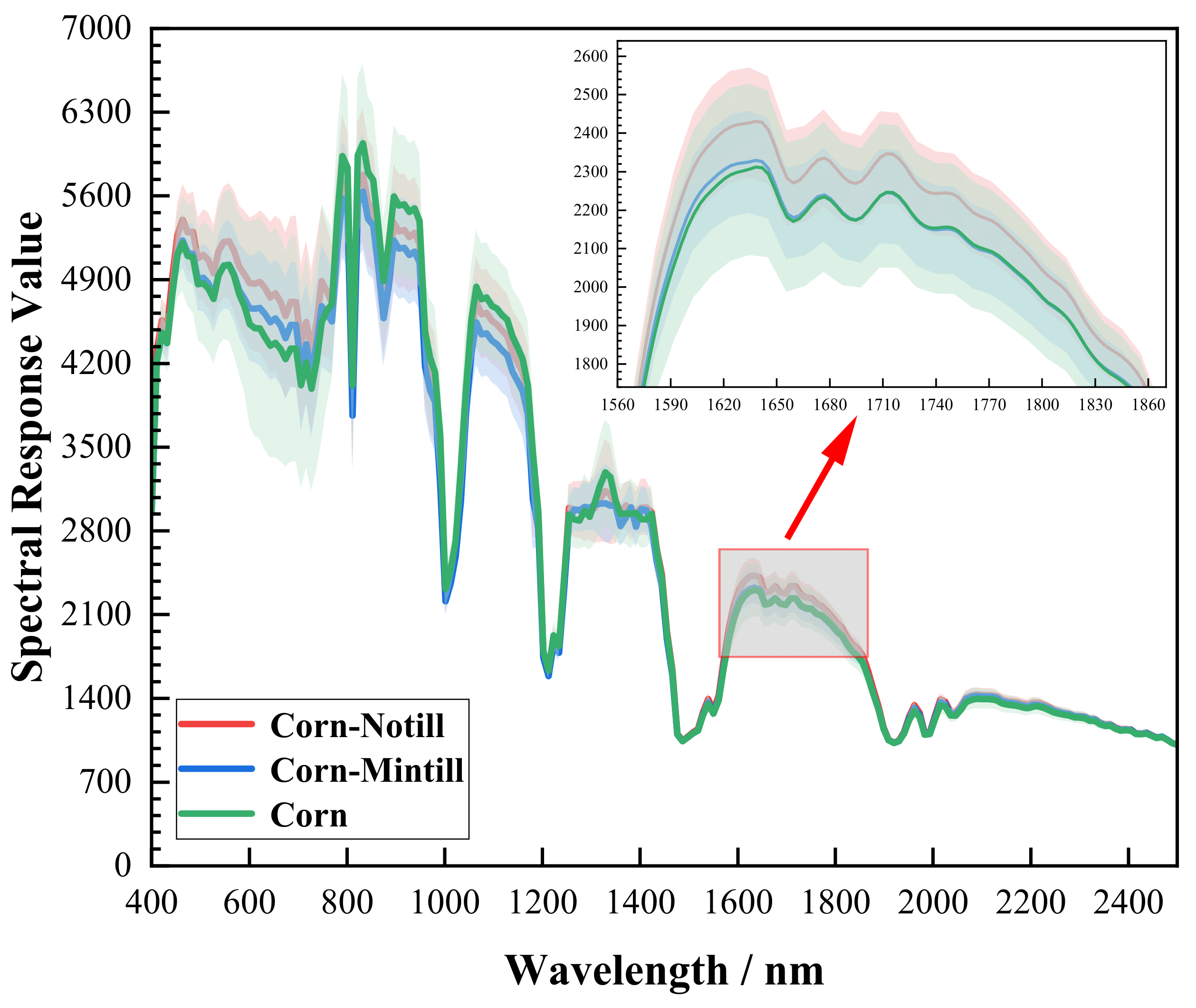
In CNN-based classification networks, spectral weighting mechanisms are often used to enhance representative spectral features. They learn an importance weight for each band based on spectral response values. Spectral variability causes samples of the same class to have different spectral responses, while samples of different classes have similar spectral characteristics. As shown in Figure 1, this section presents the average spectral response values and standard deviations of the Corn-Notill, Corn-Mintill, and Corn classes in the Indian dataset. The results indicate that the three types of ground objects have highly similar spectral curves. Moreover, the spectral distributions of samples of the three types of ground objects overlap with each other. However, current spectral weighting mechanisms generally learn band weights based on spectral responses and ignore class information. This makes it difficult for them to deal with inter-class spectral overlap and accurately distinguish samples with similar spectra, but which belong to different classes.

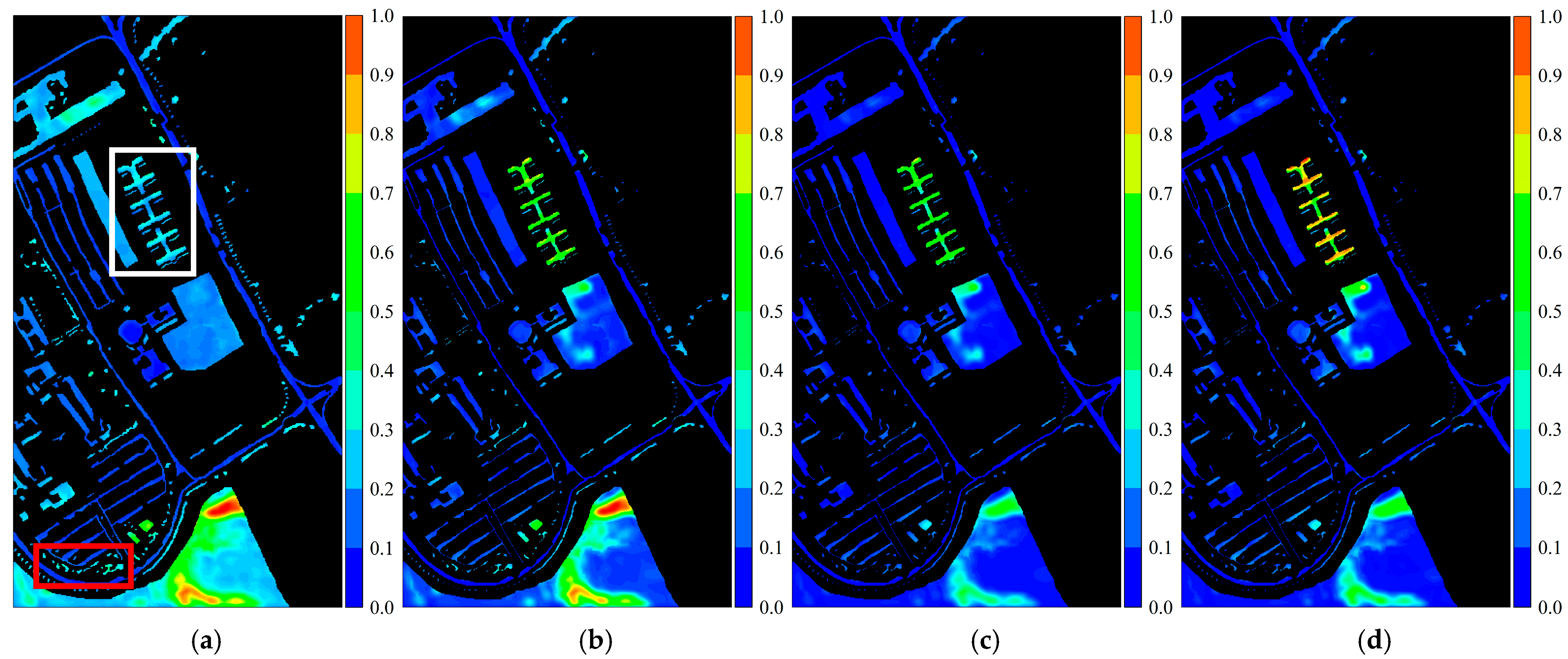
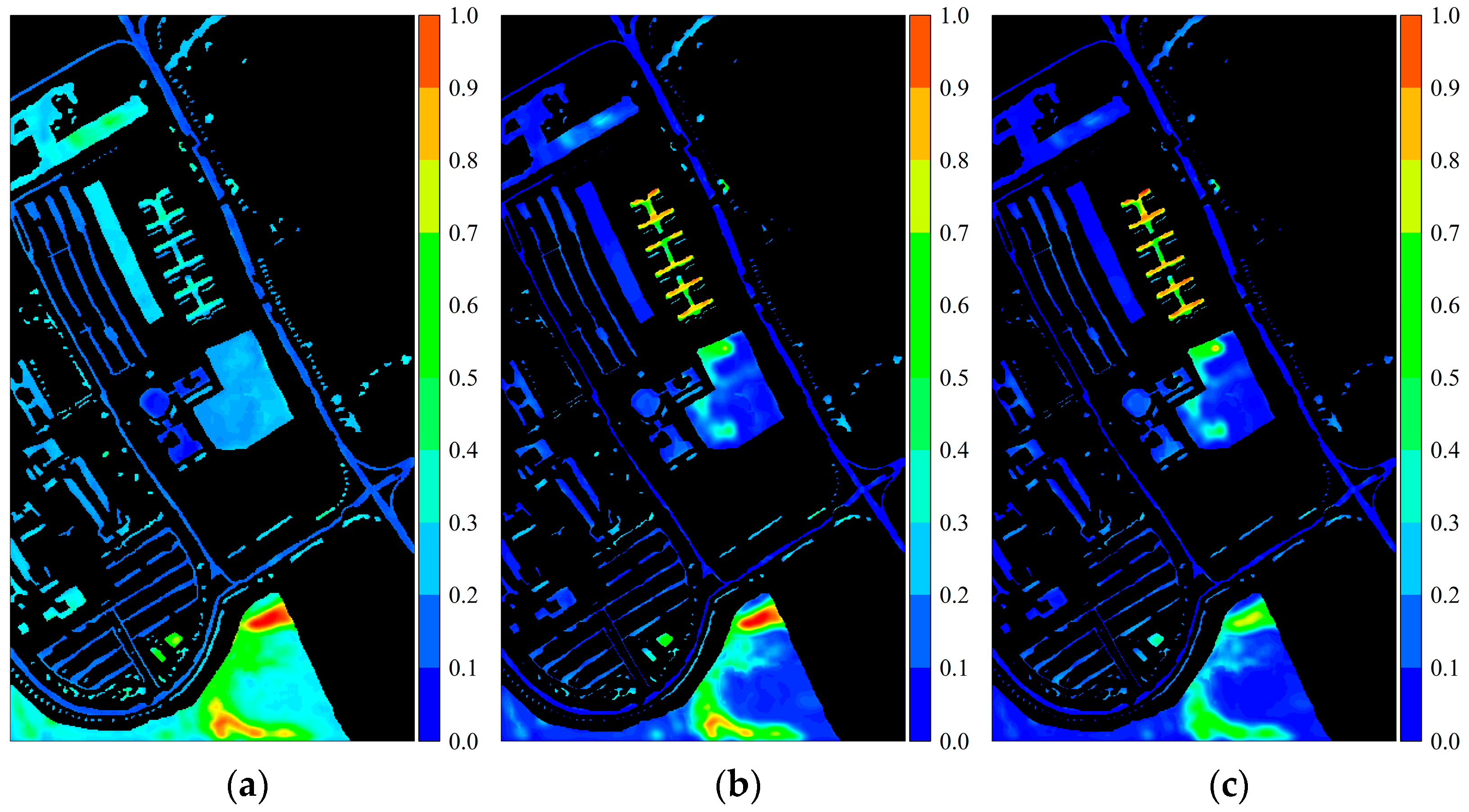
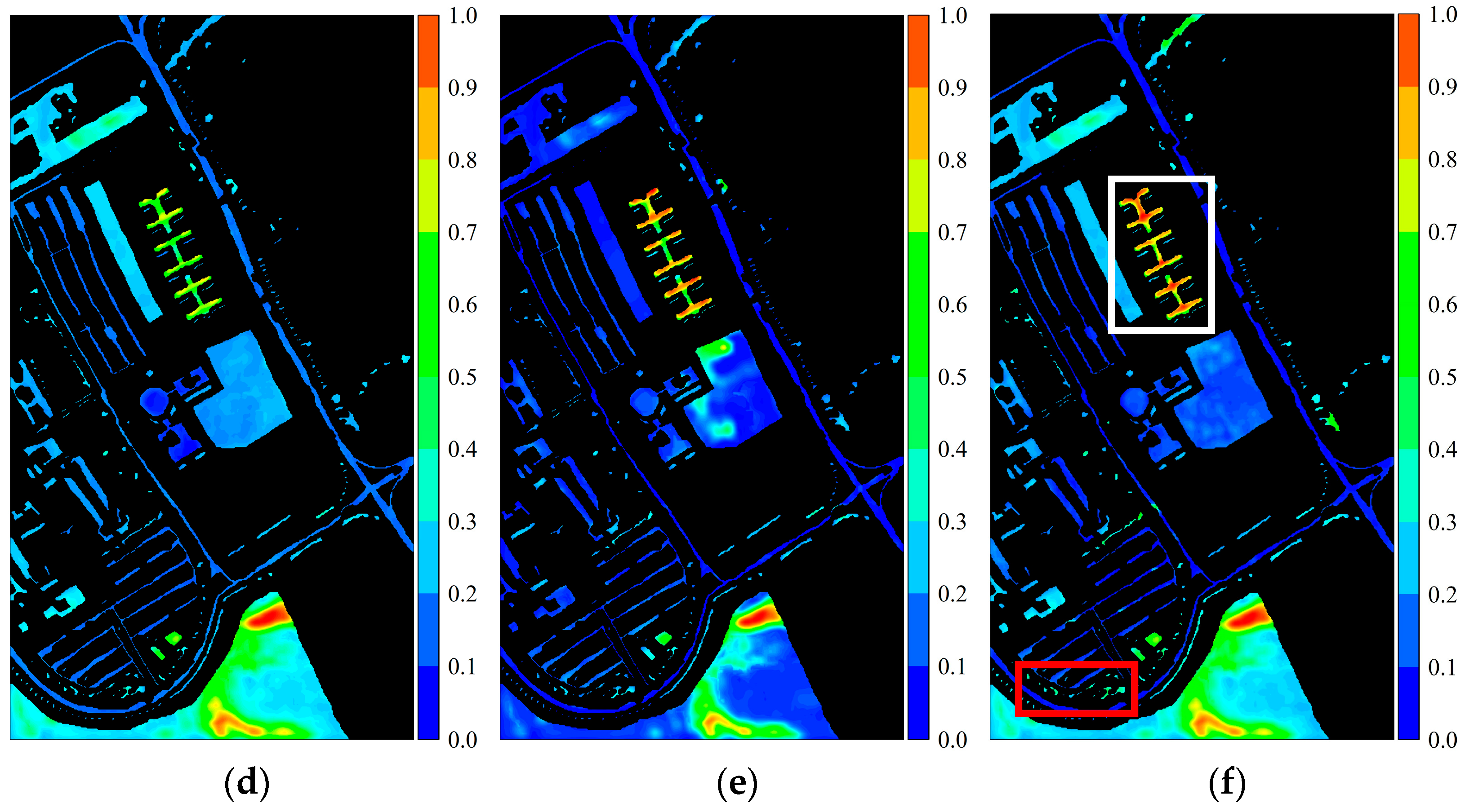
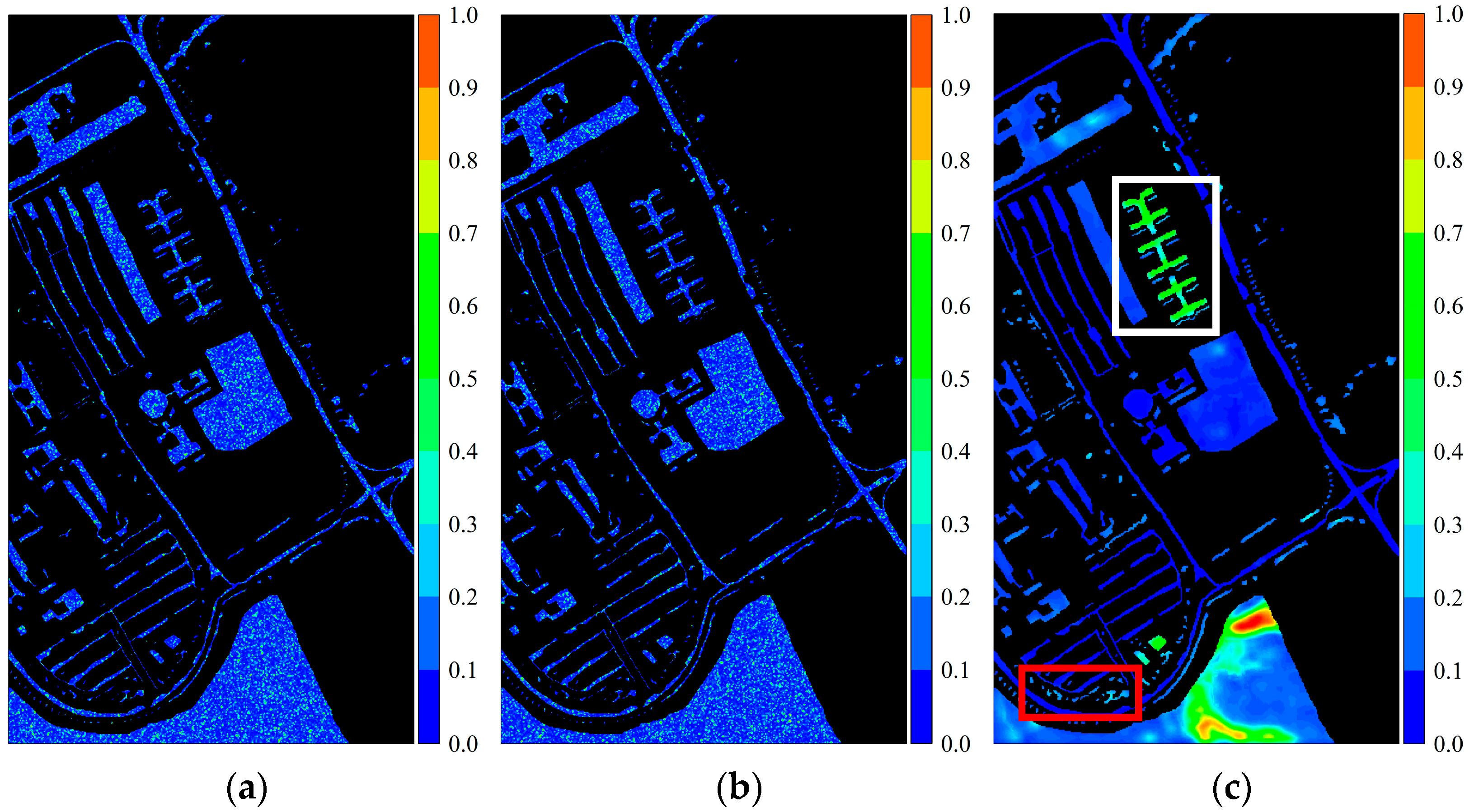
In HSI classification, the multiscale CNN uses convolutional kernels with different receptive fields to extract features at different scales. This helps the classification network to better model spatial information and capture diverse spatial distribution patterns of ground objects. As shown in Figure 2, this section presents the activation response heatmaps obtained from the PaviaU dataset using different convolutional kernels. The activation response represents the effective feature information obtained at a specific scale. The larger the activation response, the more effective the feature information. The red and white boxes in Figure 2a represent the Trees and Painted Metal Sheets classes, respectively. On small-scale features extracted by $3\times 3$ convolutional kernel, the Trees class has  a larger activation response. Its activation response gradually decreases as  the receptive field increases. The Painted Metal Sheets class has a smaller  activation response on small-scale features extracted by $3\times 3$ convolutional kernel. As the receptive  field increases, its activation response gradually increases. In particular, the  Trees and Painted Metal Sheets classes have completely different activation  responses on features extracted by $3\times 3$ convolutional kernel and features  extracted by $9\times 9$ convolutional kernel. In this case,  directly fusing features from all scales may cause the ground object with a higher  activation response at a specific scale to be weakened by features at other  scales. This easily leads to semantic degradation and affects classification  performance.

2.3. Transformer in HSI Classification

The limited receptive field makes it difficult for CNN to model long-range dependency. Recently, transformer based on the multi-head self-attention (MHSA) mechanism [45] has been applied in HSI classification to capture long-range context [46,47,48,49,50].

Let the input feature be $F\in {\mathbb{R}}^{H_F\times W_F\times C}$, where $H_F$, $W_F$, and $C$ are the feature height, width, and channel dimension. As shown in Figure 3, the self-attention mechanism first uses three linear projection layers to generate the query matrix $Q\in {\mathbb{R}}^{H_F\times W_F\times D}$, key matrix $K\in {\mathbb{R}}^{H_F\times W_F\times D}$, and value matrix $V\in {\mathbb{R}}^{H_F\times W_F\times D}$ from the input feature $F$, as follows:

$$Q=F{W}^Q,\mathrm{ }\mathrm{ }\mathrm{ }K=F{W}^K,\mathrm{ }\mathrm{ }\mathrm{ }V=F{W}^V$$

(1)

where $W^Q,W^K,W^V\in {\mathbb{R}}^{D\times D}$ are three learnable projection matrixes.

According to Figure 3, the self-attention mechanism can be formulated as follows:

$$A=Attention\left(Q,K,V\right)=softmax\left({\displaystyle \frac{Q{K}^T}{\sqrt{D}}}\right)V$$

(2)

MHSA first uses multiple $W_h^Q$, $W_h^K$, and $W_h^V$ to generate $Q_h$, $K_h$, and $V_h$. Then, $Q_h$, $K_h$, and $V_h$ are used to calculate the self-attention according to Equation (2) in the hth head. Finally, the self-attention calculated in all heads is concatenated, and a linear projection layer is used to obtain the output features of MHSA, as follows:

$$MHSA=Concat\left(A_1,\dots ,A_H\right)W^o$$

(3)

where $H$ is the number of heads; $W^o$ is a learnable linear projection matrix; and $A_h$ denotes the self-attention calculated in the hth head, which can be formulated as

$$A_h=Attention\left(Q_h,K_h,V_h\right)$$

(4)

HSI classification networks usually take a square patch as input. This results in the input patch containing background noise and heterogeneous pixels that do not belong to the same class as the center pixel. The interference information introduced by these pixels affects the classification decision of the center pixel. As shown in

Table 1. The number of homogeneous patches and heterogeneous patches in five public HSI datasets. The homogeneous patch indicates that all pixels in the patch belong to the same class. The heterogeneous patch means that the patch contains background noise or heterogeneous pixels.

Dataset	Indian	Houston	HongHu	PaviaU	Salinas
Homogeneous Patches	1402	32	10,740	26,561	9179
Heterogeneous Patches	8847	14,997	375,953	27,568	33,597

, this section reports the number of homogeneous patches and heterogeneous patches in five public HSI datasets. The results show that the number of heterogeneous patches is significantly greater than the number of homogeneous patches.

To reduce the impact of background noise and heterogeneous pixels, various center attention mechanisms have been proposed. They measure correlations between the center pixel and its neighboring pixels. This enables the classification network to obtain discriminative spectral–spatial information from neighboring pixels that have high correlation with the center pixel. However, current center attention mechanisms usually neglect their combination with convolutional feature extraction. They take the center attention mechanism as an independent feature processing module. This may cause interference information to continue accumulate in the convolutional layer, thereby reducing the feature representation capability and overall classification performance.

3. Class-Aware Progressive Multiscale Fusion Transformer

Aiming at the above problems, a class-aware progressive multiscale fusion transformer (CPMFFormer) is proposed. It is a deep learning network based on AI reasoning. CPMFFormer enhances AI’s intelligent decision capabilities through class-aware spectral discrimination and progressive semantic fusion mechanism.

3.1. Overall Framework

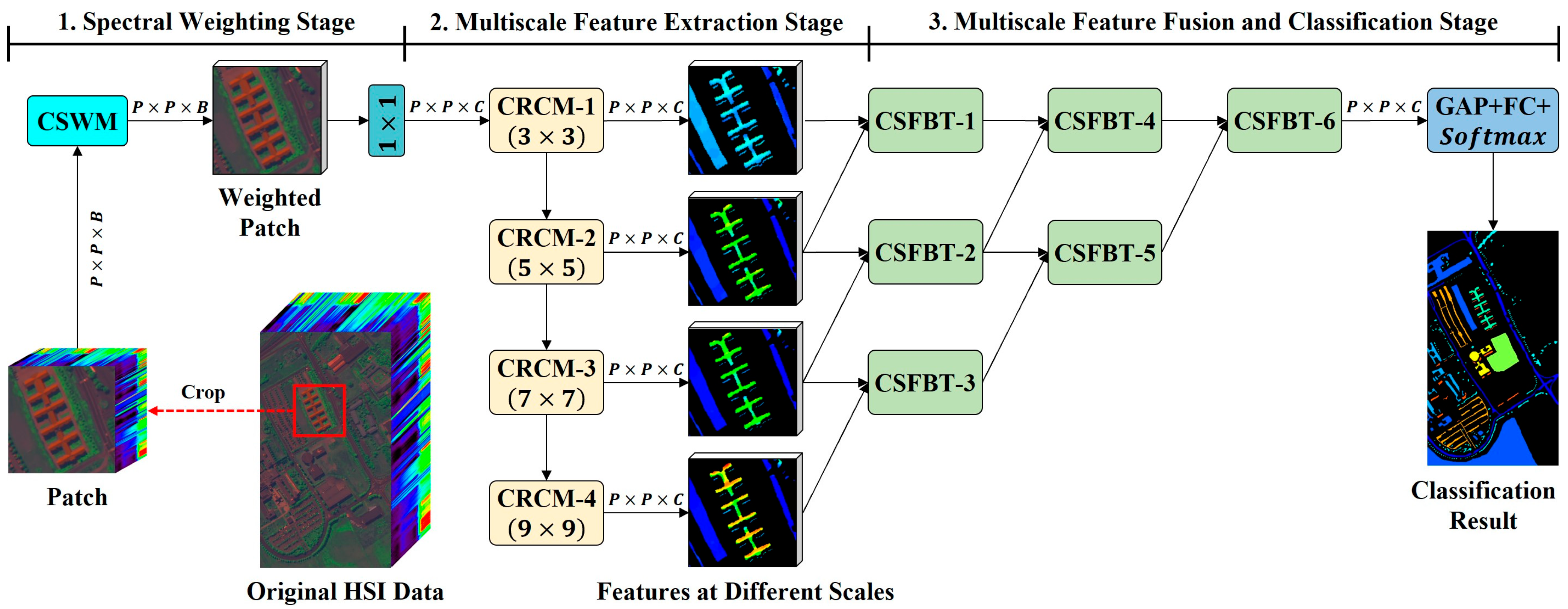
As shown in Figure 4, CPMFFormer consists of the spectral weighting stage, multiscale feature extraction stage, and multiscale feature fusion and classification stages.

(1)

In the spectral weighting stage, CPMFFormer first crops a patch of size $P\times P\times B$ centered at the pixel $x_i$ from HSI. Then, the patch is fed into CSWM to generate a weighted patch of size $P\times P\times B$. Finally, the weighted patch is resized to $P\times P\times C$ using a $1\times 1$ convolutional layer, where $C$ is the feature channel dimension.

(2)

In the multiscale feature extraction stage, CPMFFormer uses four CRCMs with different receptive fields to extract features at different scales of size $P\times P\times C$. Moreover, CRCM introduces a center feature calibration layer (CFCL) to suppress interference information and enhance the representation capability for the center pixel.

(3)

In the multiscale feature fusion and classification stage, CPMFFormer uses the cross-scale fusion bottleneck transformer (CSFBT) to gradually fuse adjacent scale features. Moreover, a global average pooling (GAP) layer, a fully connected (FC) layer, and a $Softmax$ function are used to predict the class label of the center pixel, as follows:

$${\widehat{y}}_i=Softmax\left(FC\left(GAP\left(F_{OUT}\right)\right)\right)$$

(5)

where $F_{OUT}$ is the output features of CSFBT-6 and ${\widehat{y}}_i$ is the predicted class probability.

3.2. Class-Aware Spectral Weighting Module

In the first stage shown in Figure 4, to accurately distinguish samples with similar spectra but which belong to different classes, CSWM introduces class information into the spectral weighting mechanism to obtain class-specific spectral weights.

As shown in Figure 5, CSWM consists of an aggregation operation, a spectral weight learning block, and a class consistency loss function. Affected by spectral variability, pixels of the same class may exhibit significant differences across spectral bands. To mitigate this intra-class spectral fluctuation, CSWM first measures similarity relationships between bands in the spectral domain through the aggregation operation. This operation calculates the inter-band similarity matrix $A\in {\mathbb{R}}^{B\times B}$ using the Euclidean distance, as follows:

$$A=1-{\displaystyle \frac{S-min\left(S\right)}{max\left(S\right)-min\left(S\right)}}$$

(6)

where $S\in {\mathbb{R}}^{B\times B}$ is the distance matrix which can be formulated as follows:

$$S_{ij}={‖B_i-B_j‖}^2=\sum _{h,w=1}^{H, W}{\left(B_{hwi}-B_{hwj}\right)}^2$$

(7)

where $H$ and $W$ are the height and width of the HSI. $B_i$ and $B_j$ are two bands.

Next, a normalized graph Laplacian matrix $L$ is constructed, as follows:

$$L=G^{-1/2}\left(I-A\right)G^{-1/2}$$

(8)

where $I$ and $G$ are the identity matrix and degree matrix, respectively.

By smoothing the input patch $X_i$ using the graph Laplacian matrix $L$, the aggregated patch ${\tilde{X}}_i$ can be obtained. The calculation process can be formulated as follows:

$${\tilde{X}}_i=X_{i}L$$

(9)

This process can be viewed as building a fully connected graph between similar bands in the spectral domain. This allows spectral information to be propagated between semantically similar band features and helps mitigate random shifts caused by spectral fluctuations. In addition, CSWM introduces a learnable matrix $W\in {\mathbb{R}}^{B\times B}$ to adaptively weight the aggregated patches. This further enhances discriminative band combination. The final smoothing output in the spectral domain can be formulated as follows:

$${\overline{X}}_i={\tilde{X}}_{i}W$$

(10)

Through the above operations, CSWM can automatically learn the dynamic correlations between bands and effectively reduce the interference of noise bands.

To highlight key band information, CSWM uses the channel attention mechanism [51] to weight the spectral vector. Specifically, CSWM uses a global max pooling (GMP) layer and a GAP layer in parallel to generate two spatial context descriptors, as follows:

$$D_{GMP}=GMP\left({\overline{X}}_i\right),\mathrm{ }\mathrm{ }\mathrm{ }{D}_{GAP}=GAP\left({\overline{X}}_i\right)$$

(11)

These two descriptors are fed into a shared multi-layer perceptron (MLP). The spectral weight $w_i\in {\mathbb{R}}^{1\times 1\times B}$ is obtained through a nonlinear activation function, as follows:

$$w_i=\sigma \left(MLP\left(D_{CMP}\right)+MLP\left(D_{CAP}\right)\right)$$

(12)

where $\sigma \left(·\right)$ is the $Sigmoid$ function. The final weighted output can be formulated as follows:

$${\widehat{X}}_i={\overline{X}}_i·w_i+X_i$$

(13)

Relying only on the spectral distribution for weighting may result in band weights of different ground objects being highly similar. To enhance class-discriminative spectral features, CSWM introduces a class consistency loss, as follows:

$${\mathcal{L}}_C={\displaystyle \frac{1}{M}}\sum _{i=1}^M{‖C_{y_i}-w_i‖}_2^2$$

(14)

where $M$ is the batch size; $l_i$ is the class label of the ith patch; and $C_{y_i}$ is a learnable matrix that represents the spectral weight center of the y_ith class.

This constraint forces the spectral weights of samples of the same class to converge to the same center during training, thereby enhancing intra-class consistency.

By introducing spectral aggregation, attention weighting, and class constraints, CSWM improves the discriminative power of spectral features. It not only smooths spectral fluctuations and suppresses redundant bands but also achieves class-level spectral selectivity. This provides more discriminative input features for subsequent modules.

3.3. Center Residual Convolution Module

In the second stage shown in Figure 4, to extract features at different scales and reduce the impact of abnormal pixels on the classification decision of the center pixel, this section designs CRCM based on group convolution and a center attention mechanism.

As shown in Figure 6, CRCM is composed of two bottleneck residual blocks. Let the input feature size be $P\times P\times C$. The bottleneck residual block first uses a $1\times 1$ convolutional layer to reduce the feature channel dimension. The reduced feature size is $P\times P\times C_R$. Second, a $k_t\times k_t$ group convolutional layer is used to extract features at the tth scale. A batch normalization and a rectified linear unit (ReLU) function are used for feature normalization and nonlinear enhancement. Then, CRCM introduces CFCL to model the dependencies between the center pixel and its neighboring pixels. Finally, a $1\times 1$ convolutional layer is used to restore the feature channel dimension.

As shown in Figure 4, to capture spatial structure information, CPMFFormer uses four CRCMs with convolution kernel sizes of $3\times 3$, $5\times 5$, $7\times 7$, and $9\times 9$, respectively, to extract features at different scales. The increase in the convolutional kernel size leads to an increase in the computational complexity. Considering that group convolution can reduce computational cost by decreasing the feature channel dimension in each group. Therefore, this paper adaptively allocates the feature channel dimension $C_t$ in each group based on the convolutional kernel size, which can be formulated as follows:

$$C_t=C_R/2^{{\displaystyle \frac{k_t-1}{2}}}$$

(15)

This adaptive strategy enables CRCM to achieve abundant multiscale perception while remaining lightweight. This helps improve the applicability of CPMFFormer.

The core idea of CFCL is to simulate the attention mechanism, which strengthens the key region features by calculating dependencies between the center pixel and its neighboring pixels. As shown in Figure 7, CFCL first calculates an inner product attention weight $A^C\in {\mathbb{R}}^{P\times P}$ between each neighboring pixel and the center pixel, as follows:

$$A_{ij}^C=F_{ij}·F_{i_c{j}_c}+R_{ij}^C$$

(16)

where $\left(i,j\right)$ is the spatial position of the neighboring pixel $x_n$; $\left(i_c,j_c\right)$ is the spatial position of the center pixel $x_c$; $A_{ij}^C$ is the dependency between the neighboring pixel $x_n$ and the center pixel $x_c$; $F_{ij}$ represents the feature vector of the neighboring pixel $x_n$; $F_{ij}$ represents the feature vector of the center pixel $x_c$; and $R_{ij}^C$ is the relative center position encoding of the neighboring pixel $x_n$, which can be formulated as follows:

$$R_{ij}^C=1/\left(1+\sqrt{{\left|\right|i-i_c\left|\right|}^2+{\left|\right|j-j_c\left|\right|}^2}\right)$$

(17)

Then, a center dependency matrix $S^C\in {\mathbb{R}}^{P\times P}$ is obtained using a $Softmax$ normalization. The final output calibration features $F^C\in {\mathbb{R}}^{P\times P\times C_R}$ can be expressed as follows:

$$F_{ij}^C=S_{ij}^C·F_{ij}$$

(18)

The above process can be viewed as a weighted summation for the neighboring pixels, which enhances the feature representation for regions that are highly correlated with the center pixel. This helps to improve the distinguishability of the center pixel.

Compared with the existing center attention mechanism, this section embeds CFCL into CRCM at different spatial scales. This achieves hierarchical suppression of interference information. Among them, shallow CFCL suppresses local noise, while deep CFCL enhances structural boundaries. This module not only effectively resists interference from abnormal pixels but also enhances spatial continuity. This provides a semantically consistent feature representation for subsequent cross-scale fusion.

3.4. Cross-Scale Fusion Bottleneck Transformer

In the third stage shown in Figure 4, after completing the multiscale spatial feature extraction, CPMFFormer needs to effectively fuse features at different scales to fully explore cross-scale complementary information. Therefore, this paper builds a progressive multiscale fusion strategy. This strategy takes CSFBT as its core, which achieves a smooth semantic transition by gradually fusing adjacent scale features.

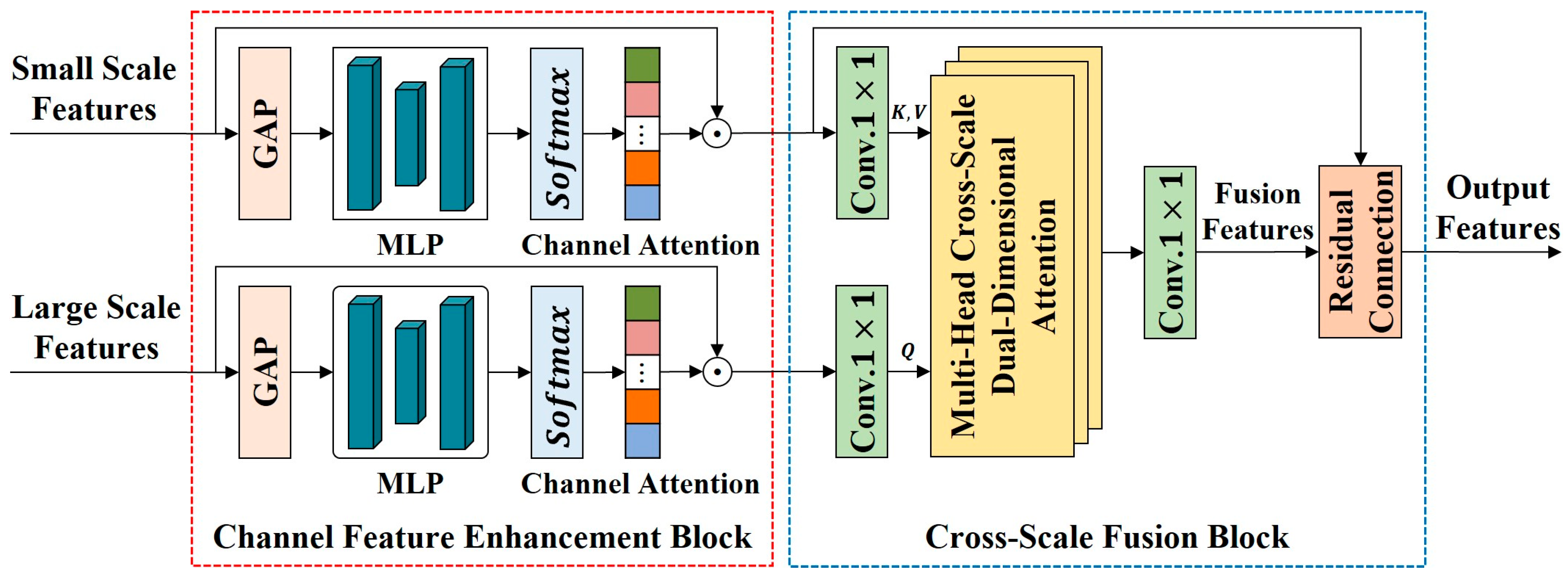
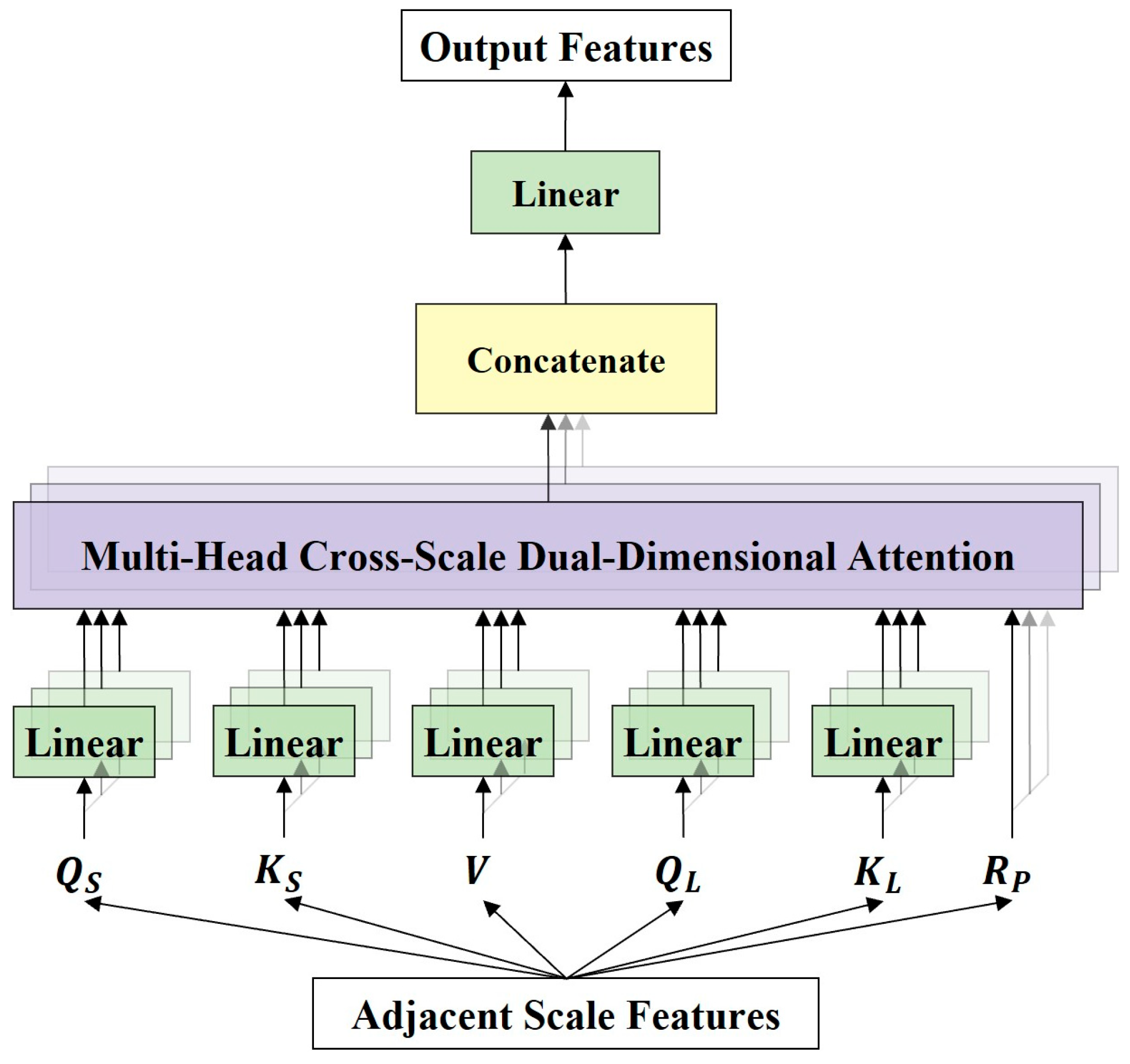
As shown in Figure 8, CSFBT takes adjacent scale features as input. It consists of a channel feature enhancement block (CFEB) and a cross-scale fusion block (CSFB). CFEB enhances valuable channel features. CSFB uses a multi-head cross-scale dual-dimensional attention (MHCSD2A) mechanism to promote semantic interaction and information redistribution across adjacent scale features from both spatial and channel dimensions.

The design idea of CFEB is to weight the channel features in adjacent scale features. This enables CFEB to highlight information-rich channel responses. For small-scale features $F_S\in {\mathbb{R}}^{P\times P\times C}$ and large-scale features $F_L\in {\mathbb{R}}^{P\times P\times C}$, CFEB first uses two GAP layers to obtain two spatial context descriptors $D_{GAP}^S,D_{GAP}^L\in {\mathbb{R}}^{1\times 1\times C}$, as follows:

$$D_{GAP}^S=GAP\left(F_S\right), D_{GAP}^L=GAP\left(F_L\right)$$

(19)

Then, two MLPs are used to generate the channel attention weights $w_S\in {\mathbb{R}}^{1\times 1\times C}$ and $w_L\in {\mathbb{R}}^{1\times 1\times C}$ for small-scale and large-scale features, respectively, as follows:

$$w_S=\sigma \left(MLP\left(D_{GAP}^S\right)\right), w_L=\sigma \left(MLP\left(D_{GAP}^L\right)\right)$$

(20)

where $\sigma \left(·\right)$ denotes the $Softmax$ function.

Finally, the weight vectors $w_S$ and $w_L$ are used to reweight small-scale features and large-scale features, respectively, which can be formulated as follows:

$$F_S^{\prime }=w_S·F_S, F_L^{\prime }=w_L·F_L$$

(21)

CFEB can effectively suppress invalid channel features and make the input adjacent scale features more focused and discriminative in the channel dimension.

Next, CSFB is used to capture cross-scale dependencies from both spatial and channel dimensions. As shown in Figure 8, CSFB first uses two $1\times 1$ convolutional layers to reduce the feature channel dimension. The reduced small-scale and large-scale features are denoted as $F_S^{″}, F_L^{″}\in {\mathbb{R}}^{P\times P\times C^{\prime }}$. Then, $F_S^{″}$ and $F_L^{\prime \prime }$ are fed into MHCSD2A to integrate complementary information across different scales. Finally, a $1\times 1$ convolutional layer is used to restore the feature channel dimension and obtain the fusion features.

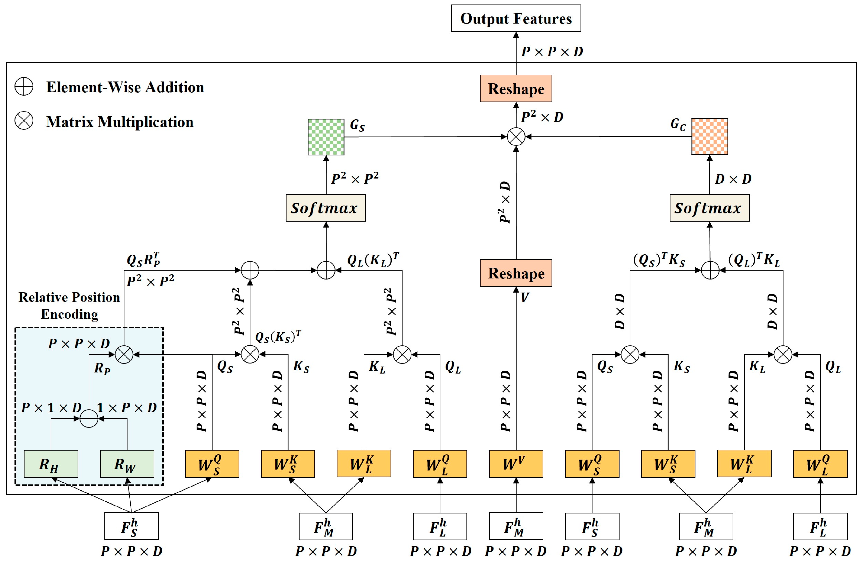
Let MHCSD2A have $H$ heads and the feature channel dimension in each head be $D$. As shown in Figure 9, MHCSD2A projects $F_S^{″}$ and $F_L^{″}$ into $\left\{F_S^1,\dots ,F_S^H\right\}\in {\mathbb{R}}^{P\times P\times D}$ and $\left\{F_L^1,\dots ,F_L^H\right\}\in {\mathbb{R}}^{P\times P\times D}$, respectively. $F_S^h$ and $F_L^h$ are input into the cross-scale dual-dimensional attention (CSD2A) mechanism to enhance scale-specific information. As shown in Figure 10, CSD2A adds $F_S^h$ and $F_L^h$ to obtain multiscale features $F_M^h\in {\mathbb{R}}^{P\times P\times D}$. $F_M^h$ contains both small-scale detail information and large-scale semantic information. CSD2A uses two $1\times 1$ convolutional layers to obtain $Q_S\in {\mathbb{R}}^{P\times P\times D}$ and $Q_L\in {\mathbb{R}}^{P\times P\times D}$ from $F_S^h$ and $F_L^h$, respectively. Meanwhile, CSD2A uses three $1\times 1$ convolutional layers to obtain $K_S\in {\mathbb{R}}^{P\times P\times D}$, $K_L\in {\mathbb{R}}^{P\times P\times D}$, and $V\in {\mathbb{R}}^{P\times P\times D}$ from $F_M^h$, which can be formulated as follows:

$$Q_S=F_S^h{W}_S^Q, Q_L=F_L^h{W}_L^Q$$

(22)

$$K_S=F_M^h{W}_S^K, K_L=F_M^h{W}_L^K, V=F_M^h{W}^V$$

(23)

where $W_S^Q,W_L^Q,W_S^K,W_L^K,W^V\in {\mathbb{R}}^{D\times D}$ are five learnable linear projection matrices.

On the spatial dimension, CSD2A first multiplies $Q_S$ and ${\left(K_S\right)}^T$ to obtain the small-scale spatial attention matrix $Z_S^S=Q_S{\left(K_S\right)}^T\in {\mathbb{R}}^{P^2\times P^2}$. The larger the value in $Z_S^S$, the more spatially informative the position is for small-scale features. Then, $Q_L$ and ${\left(K_L\right)}^T$ are multiplied to obtain the large-scale spatial attention matrix $Z_L^S=Q_L{\left(K_L\right)}^T\in {\mathbb{R}}^{P^2\times P^2}$. The larger the value in $Z_L^S$, the more spatially informative the position is for large-scale features. Finally, $Z_S^S$ and $Z_L^S$ are added to obtain the cross-scale spatial attention matrix $Z^S=Z_S^S+Z_L^S\in {\mathbb{R}}^{P^2\times P^2}$. To better describe spatial structures, the relative position encoding $R_P\in {\mathbb{R}}^{P\times P\times D}$ is introduced into $Z^S$. In addition, a $Softmax$ function is used for normalization to obtain the cross-scale spatial dependency matrix $G_S\in {\mathbb{R}}^{P^2\times P^2}$, as follows:

$$G_S=Softmax\left({\displaystyle \frac{Q_S{\left(R_P\right)}^T+Q_S{\left(K_S\right)}^T+Q_L{\left(K_L\right)}^T}{\sqrt{D}}}\right)$$

(24)

On the channel dimension, CSD2A first multiplies ${\left(Q_S\right)}^T$ and $K_S$ to obtain the small-scale channel attention matrix $Z_S^C={\left(Q_S\right)}^T{K}_S\in {\mathbb{R}}^{D\times D}$. The larger the value in $Z_S^C$, the more channel-informative the position is for small-scale features. Second, ${\left(Q_L\right)}^T$ and $K_L$ are multiplied to obtain the large-scale channel attention matrix $Z_L^C={\left(Q_L\right)}^T{K}_L\in {\mathbb{R}}^{D\times D}$. The larger the value in $Z_L^C$, the more channel-informative the position is for large-scale features. Then, $Z_S^C$ and $Z_L^C$ are added to obtain the cross-scale channel attention matrix $Z^C=Z_S^C+Z_L^C\in {\mathbb{R}}^{D\times D}$. Meanwhile, a $Softmax$ function is used for normalization to obtain the cross-scale channel dependency matrix $G_c\in {\mathbb{R}}^{D\times D}$, which can be formulated as follows:

$$G_C=Softmax\left({\displaystyle \frac{{\left(Q_S\right)}^T{K}_S+{\left(Q_L\right)}^T{K}_L}{\sqrt{D}}}\right)$$

(25)

Finally, CSD2A multiplies $G_S$, $V$, and $G_C$ to obtain its output, as follows:

$$A_h=G_{S}V{G}_C\in {\mathbb{R}}^{P\times P\times D}$$

(26)

Next, the outputs of all heads are concatenated, and a linear projection layer is used to obtain the output of MHCSD2A. MHCSD2A with $H$ heads can be formulated as follows:

$$MHCSD2A=Concat\left(A_1,A_2,\dots ,A_H\right)W^o$$

(27)

where $W^o\in {\mathbb{R}}^{C^{\prime }\times C^{\prime }}$ represents a learnable linear projection matrix.

According to the above descriptions, MHCSD2A ensures that the fusion result can preserve small-scale detail features while integrating large-scale semantic information. This helps CPMFFormer to form a hierarchical and progressive spatial representation.

Compared with existing multiscale fusion strategies, the progressive multiscale fusion strategy not only avoids semantic conflicts between features with large-scale differences, but also maintains the continuity of semantic hierarchy across different scales. This enhances the representational power and classification robustness of CPMFFormer.

3.5. Loss Function

The loss function is used to quantify the difference between the predicted label and the actual label. By minimizing the loss function, a deep learning network can gradually adjust its parameters to make the predicted label as close to the actual label as possible. The common loss function in HSI classification is the cross-entropy loss ${\mathcal{L}}_{CE}$, as follows:

$${\mathcal{L}}_{CE}=-{\displaystyle \frac{1}{M}}{\sum }_{i=1}^{M}log\left(p_{i,l_i}\right)$$

(28)

where $p_{i,l_i}$ is the predicted probability that the ith pixel belongs to the l_ith class.

The total loss $L$ of CPMFFormer includes the class consistency loss in CSWM and the cross-entropy loss for classification, which can be formulated as follows:

$$L={\mathcal{L}}_{CE}+\tau {\mathcal{L}}_C$$

(29)

where $\tau$ is a balance parameter, which is set to 10 by trial and error.

3.6. Illustrative Example

To show CPMFFormer more clearly, this section takes the Indian dataset of size $145\times 145\times 200$ as an example to analyze its calculation process in detail. Let the input patch size be $11\times 11\times 200$ and the feature channel dimension be 128. As shown in Figure 4, a $1\times 1$ convolutional layer following the weighted patch is used to adjust the feature channel dimension. It can extract features of size $11\times 11\times 128$. Moreover, this feature is used as the input of CRCM $\left(3\times 3\right)$. The implementation processes of different modules are shown in

Table 2. The implementation process of CSWM.

Layer Name	Kernel Size	Output Size
Aggregation	-	11 × 11 × 200
Spectral Weight Learning	-	1 × 1 × 200
Element-Wise Multiplication	-	11 × 11 × 200
Element-Wise Addition	-	11 × 11× 200

,

Table 3. The implementation process of CRCM (3 × 3).

Layer Name	Kernel Size	Output Size
Conv	1 × 1	11 × 11 × 64
GConv-BN-ReLU	3 × 3	11 × 11 × 64
CFCL	-	11 × 11 × 64
Conv	1 × 1	11 × 11 × 128
Residual Connection	-	11 × 11 × 128
Conv	1 × 1	11 × 11 × 64
GConv-BN-ReLU	3 × 3	11 × 11 × 64
CFCL	-	11 × 11 × 64
Conv	1 × 1	11 × 11 × 128
Residual Connection	-	11 × 11 × 128

and

Table 4. The implementation process of CSFBT.

Layer Name	Kernel Size	Output Size
CFEB	-	11 × 11 × 128 11 × 11 × 128
Conv	1 × 1	11 × 11 × 12 11 × 11 × 12
MHCSD2A	-	11 × 11 × 12
Conv	1 × 1	11 × 11 × 128
Residual Connection	-	11 × 11 × 128

, respectively.

For ease of description, the group convolutional layer, batch normalization, and ReLU activation function are abbreviated as GConv-BN-ReLU. The convolutional layer is abbreviated as Conv. This section only shows the implementation process of CRCM (3 × 3). The implementation processes of CRCM for other scale features extraction are similar to CRCM (3 × 3), and only the group convolutional kernel size needs to be changed according to Table 3. In Table 4, CFEB and the first Conv have two output sizes. They correspond to small-scale features and large-scale features, respectively.

Finally, a GAP layer is used to compress the output features of size 11 × 11 × 128 into a feature vector of size 1 × 1 × 128. Moreover, an FC layer and a Softmax function are used to obtain the predicted class labels. In addition, the optimization solution is performed according to the loss function until the network converges. Based on the above descriptions, the implementation process of CPMFFormer is shown in Algorithm 1.

Algorithm 1: The implementation process of CPMFFormer.

Input: HSI data, ground truth, training ratio, patch size, feature channel dimension, batch size, learning rate, the number of epochs.

Output: The predicted class labels on test samples.

1. Cropping the training, validation, and test patches from the HSI data.

2. Generating the training, validation, and test labels from the ground truth.

3. For $e$ = 1 to epoches

4.  Using the CSWM to obtain the weighted input patch.

5.  Using a $1\times 1$ convolutional layer to adjust the feature channels dimension.

6.  Using CRCM to extract the features at different scales.

7.  Using CSFBT to gradually fuse adjacent scale features.

8.  Using a GAP layer, an FC layer, and a $Softmax$ function to predict the class label.

9.  Updating the network parameters using training samples.

10.  Calculating loss function using validation samples. If loss function is smaller than of last epoch, the network parameter is saved. Conversely, it will not be saved.

11. End for

12. Predict the class labels on the test set using the best network.

4. Experiments and Analysis

4.1. Dataset’s Description

To validate the effectiveness of CPMFFormer, we use five public HSI datasets to carry out the subsequent experiments, including the Indian pines dataset, Houston dataset, WHU-Hi-HongHu dataset, Pavia University dataset, and Salinas dataset. These datasets were acquired using different sensors in multiple countries and regions.

Indian pines (Indian) dataset: This dataset was taken by AVIRIS sensor on Indian pines in northwestern Indiana, USA. It contains $145\times 145$ pixels and 200 spectral bands. Its ground truth provides 10,249 labeled pixels for 16 ground objects. The types of ground objects and sample distributions in the Indian dataset are shown in

Table 5. The types of ground objects and samples distribution in the Indian datasets.

Class	Name	Training	Validation	Test	Total
1	Alfalfa	1	1	44	46
2	Corn-Notill	29	29	1370	1428
3	Corn-Mintill	17	17	796	830
4	Corn	5	5	227	237
5	Grass-Pasture	10	10	463	483
6	Grass-Trees	15	15	700	730
7	Grass-Pasture-Mowed	1	1	26	28
8	Hay-Windrowed	10	10	458	478
9	Oats	1	1	18	20
10	Soybean-Notill	20	20	932	972
11	Soybean-Mintill	50	50	2355	2455
12	Soybean-Clean	12	12	569	593
13	Wheat	5	5	195	205
14	Woods	26	26	1213	1265
15	Buildings-Grass-Trees-Drives	8	8	370	386
16	Stone-Steel-Towers	2	2	89	93
Total		212	212	9825	10,249

.

Houston dataset: This dataset was taken by ITRES CASI-1500 sensor on the Houston university in Houston, TX, USA. It contains $349\times 1905$ pixels and 144 spectral bands. Its ground truth provides 15,029 labeled pixels for 15 ground objects. The types of ground objects and sample distributions in the Houston dataset are shown in

Table 6. The types of ground objects and sample distribution in the Houston datasets.

Class	Name	Training	Validation	Test	Total
1	Healthy Grass	26	26	1199	1251
2	Stressed Grass	26	26	1202	1254
3	Synthetic Grass	14	14	669	697
4	Trees	25	25	1194	1244
5	Soil	25	25	1192	1242
6	Water	7	7	311	325
7	Residential	26	26	1216	1268
8	Commercial	25	25	1194	1244
9	Road	26	26	1200	1252
10	Highway	25	25	1177	1227
11	Railway	25	25	1185	1235
12	Parking Lot1	25	25	1183	1233
13	Parking Lot2	10	10	449	469
14	Tennis Court	9	9	410	428
15	Running Track	14	14	632	660
Total		308	308	14,413	15,029

.

WHU-Hi-HongHu (HongHu) dataset: This dataset was taken by Headwall Nano-Hyperspec sensor on Honghu city, China. It contains $940\times 475$ pixels and 270 spectral bands. Its ground truth provides 386,693 labeled pixels for 22 ground objects. The types of ground objects and sample distributions in the HongHu dataset are shown in

Table 7. The types of ground objects and sample distribution in the HongHu datasets.

Class	Name	Training	Validation	Test	Total
1	Red Roof	281	281	13,479	14,041
2	Road	71	71	3370	3512
3	Bare Soil	437	437	20,947	21,821
4	Cotton	3266	3266	156,753	163,285
5	Cotton Firewood	125	125	5968	6218
6	Rape	892	892	42,773	44,557
7	Chinese Cabbage	483	483	23,137	24,103
8	Pakchoi	82	82	3890	4054
9	Cabbage	217	217	10,385	10,819
10	Tuber Mustard	248	248	11,898	12,394
11	Brassica Parachinensis	221	221	10,573	11,015
12	Brassica Chinensis	180	180	8594	8954
13	Small Brassica Chinensis	451	451	21,605	22,507
14	Lactuca Sativa	148	148	7060	7356
15	Celtuce	21	21	960	1002
16	Film-Covered Lettuce	146	146	6970	7262
17	Romaine Lettuce	61	61	2888	3010
18	Carrot	65	65	3087	3217
19	White Radish	175	175	8362	8712
20	Garlic Sprout	70	70	3346	3486
21	Broad Bean	27	27	1274	1328
22	Tree	81	81	3878	4040
Total		7748	7748	371,197	386,693

.

Pavia University (PaviaU) dataset: This dataset was taken by ROSIS sensor on Pavia University in Pavia, Italy. It contains $610\times 340$ pixels and 103 spectral bands. Its ground truth provides 42,776 labeled pixels for 9 ground objects. The types of ground objects and sample distributions in the PaviaU dataset are shown in

Table 8. The types of ground objects and sample distribution in the PaviaU datasets.

Class	Name	Training	Validation	Test	Total
1	Asphalt	133	133	6365	6631
2	Meadows	373	373	17,903	18,649
3	Gravel	42	42	2015	2099
4	Trees	62	62	2940	3064
5	Painted Metal Sheets	27	27	1291	1345
6	Bare Soil	101	101	4827	5029
7	Bitumen	27	27	1276	1330
8	Self-Blocking Bricks	74	74	3534	3682
9	Shadows	19	19	909	947
Total		858	858	41,060	42,776

.

Salinas dataset: This dataset was taken by AVIRIS sensor on Salinas Valley in California, USA. It contains $512\times 217$ pixels and 204 spectral bands. Its ground truth provides 54,129 labeled pixels for 16 ground objects. The types of ground objects and sample distributions in the Salinas dataset are shown in

Table 9. The types of ground objects and sample distribution in the Salinas datasets.

Class	Name	Training	Validation	Test	Total
1	Broccoli Green Weeds 1	41	41	1927	2009
2	Broccoli Green Weeds 2	75	75	3576	3726
3	Fallow	40	40	1896	1976
4	Fallow Rough Plow	28	28	1338	1394
5	Fallow Smooth	54	54	2570	2678
6	Stubble	80	80	3799	3959
7	Celery	72	72	3435	3579
8	Grapes Untrained	226	226	10,819	11,271
9	Soil Vineyard Develop	125	125	5953	6203
10	Corn Senesced Green Weeds	66	66	3146	3278
11	Lettuce Romaine 4 wk.	22	22	1024	1068
12	Lettuce Romaine 5 wk.	39	39	1849	1927
13	Lettuce Romaine 6 wk.	19	19	878	916
14	Lettuce Romaine 7 wk.	22	22	1026	1070
15	Vineyard Untrained	146	146	6976	7268
16	Vineyard Vertical Trellis	37	37	1733	1807
Total		1092	1092	51,945	54,129

.

4.2. Experimental Setup

Experiment Overview: To comprehensively validate the advancement and effectiveness of CPMFFormer, this section conducts the following experiments:

(1)

Parameters sensitivity analysis: This part of the experiment is used to explore the impact of important hyperparameters on network learning behavior and classification performance, which determines the appropriate parameter setting range.

(2)

Quantitative comparison: This part of the experiment is used to compare the classification performance obtained by the proposed network and existing methods on different datasets, which validates the competitiveness of CPMFFormer.

(3)

Full-scene visualization: This part of the experiment uses the complete classification results to evaluate spatial coherence and boundary retention, which intuitively reflects the expression capabilities of different networks for complex ground objects.

(4)

Network stability evaluation: This part of the experiment uses different training samples sizes to evaluate the classification performance changes in the proposed network and existing methods, which validates the reliability of CPMFFormer.

(5)

Network complexity and inference efficiency: This part of the experiment is used to measure the computational resource requirements and running speed of different networks, which evaluates the practical application prospects of CPMFFormer.

(6)

Ablation studies: This part of the experiment is mainly used to analyze the specific functions and independent contributions of each core design, which clarifies the role of different components in the feature extraction and fusion process.

(7)

Expandability analysis: This part of the experiment analyzes the value of semi-supervised learning and its improvement on classification performance, which provides a theoretical and experimental foundation for future research work.

Evaluation Metrics: In the following experiments, we use three common metrics to evaluate the classification performance of CPMFFormer, including the overall accuracy (OA), average accuracy (AA), and Kappa ($\kappa$) coefficient. OA is the ratio of the correctly  classified samples to all labeled samples. AA represents the average  classification accuracy across all classes. $\kappa$ measures the consistency between the predicted result  and ground truth. Furthermore, we adopt the Moran’s I (MI), boundary F1 score  (BF1), and structural similarity index measure (SSIM) to evaluate the spatial  coherence and boundary retention of the classification results of different  networks.

Implementation Details: All codes are implemented on the PyTorch platform. The basic hardware configurations are Intel Xeon Platinum 8358 CPU 2.60 GHz and NVIDIA A800 GPU 80 GB. The basic software configurations are Python 3.8, PyTorch 2.4, and CUDA v11.8. CPMFFormer is trained using an Adam optimizer. The initial learning rate is set to 0.003, the decay rate is (0.9, 0.999), and the fuzziness factor is 1e−8. The training epoch is set at 200 and the learning rate is dynamically adjusted every 15 epochs using cosine annealing. The comparison networks are set using the optimal parameters based on the recommendations in their papers and are trained to achieve the best classification performance using five public HSI datasets to the maximum extent possible. We repeat the experiment five times on each HSI dataset to eliminate the impact caused by the randomness and report the average classification performance $\pm$ standard deviation.

4.3. Parameters Sensitivity Analysis

The sensitivity analysis for the batch size: The batch size affects network training stability, convergence speed, and classification performance. A small batch size may introduce more gradient noise and lead to training instability. A large batch size may reduce the generalization performance of the classification network due to the dilution caused by the data diversity in each batch. As shown in Figure 11, to determine the optimal batch size, this paper sets the batch size to 16, 32, 48, 64, 80, and 96. According to the experimental results, when the batch size is 48, the Indian, Houston, HongHu, and PaviaU datasets reach the optimal evaluation metrics. Moreover, when the batch size is 48 or 64, the PaviaU dataset exhibits similar classification performance. In subsequent experiments, this paper uniformly sets the batch size to 48 for all HSI datasets.

The sensitivity analysis for the learning rate: The learning rate determines the update step of network parameters and plays a crucial role in the stability and convergence of network training. A small learning rate results in slow convergence and makes it difficult for the classification network to obtain optimal parameters. A large learning rate may lead to oscillation or even divergence in the training process, thereby reducing the classification performance. As shown in Figure 12, to determine the optimal learning rate, this paper sets the learning rate to 0.0003, 0.001, 0.003, 0.01, and 0.03. The experimental results show that when the learning rate is 0.003, the Indian and Houston datasets have the best classification performance. In contrast, the learning rate has a relatively small impact on the other three HSI datasets. In subsequent experiments, this paper uniformly sets the learning rate to 0.003 for all HSI datasets.

The sensitivity analysis for the number of CRCM: The number of CRCMs is related to the spatial information captured by the classification network. Fewer CRCMs make it difficult for CPMFFormer to effectively suppress interference pixels. More CRCMs may introduce redundant information and increase the computational cost. As shown in

Table 10. Impact of the number of CRCM on classification performance. The optimal results are in red.

Datasets	Metrics	CRCM = 2	CRCM = 3	CRCM = 4	CRCM = 5	CRCM = 6
Indian	OA (%)	93.70 ± 1.06	94.83 ± 0.92	94.85 ± 0.69	94.84 ± 0.83	93.94 ± 0.78
	AA (%)	92.88 ± 0.97	93.48 ± 1.36	94.35 ± 0.61	94.33 ± 0.60	92.93 ± 1.21
	κ (%)	92.82 ± 1.21	94.12 ± 1.04	94.13 ± 0.80	94.14 ± 0.95	93.09 ± 0.89
Houston	OA (%)	95.76 ± 0.62	95.88 ± 0.73	95.93 ± 0.36	95.91 ± 0.40	95.29 ± 0.52
	AA (%)	95.93 ± 0.81	96.01 ± 0.73	96.06 ± 0.26	95.92 ± 0.53	95.51 ± 0.64
	κ (%)	95.42 ± 0.67	95.55 ± 0.78	95.61 ± 0.39	95.60 ± 0.44	94.91 ± 0.56
HongHu	OA (%)	99.53 ± 0.04	99.50 ± 0.04	99.53 ± 0.03	99.50 ± 0.05	99.49 ± 0.05
	AA (%)	98.92 ± 0.20	98.83 ± 0.16	98.99 ± 0.10	98.82 ± 0.20	98.68 ± 0.06
	κ (%)	99.40 ± 0.05	99.37 ± 0.04	99.41 ± 0.04	99.36 ± 0.07	99.24 ± 0.06
PaviaU	OA (%)	99.45 ± 0.12	99.45 ± 0.22	99.50 ± 0.06	99.48 ± 0.13	99.35 ± 0.09
	AA (%)	98.95 ± 0.27	98.88 ± 0.45	99.02 ± 0.10	99.01 ± 0.20	98.74 ± 0.14
	κ (%)	99.27 ± 0.15	99.27 ± 0.29	99.34 ± 0.08	99.31 ± 0.18	99.13 ± 0.12
Salinas	OA (%)	99.81 ± 0.12	99.77 ± 0.13	99.84 ± 0.06	99.84 ± 0.06	99.75 ± 0.13
	AA (%)	99.81 ± 0.13	99.79 ± 0.08	99.84 ± 0.05	99.86 ± 0.02	99.75 ± 0.09
	κ (%)	99.79 ± 0.14	99.74 ± 0.14	99.82 ± 0.07	99.82 ± 0.07	99.72 ± 0.15

, to determine the optimal number of CRCM, this paper sets the number of CRCM to 2, 3, 4, 5, and 6. The experimental results show that when the number of CRCMs is 4, the Indian dataset achieves the best OA and AA. The Houston, HongHu, and PaviaU datasets reach the optimal evaluation metrics. The Salinas dataset has the optimal OA and $\kappa$ When the  number of CRCMs is 5, the Indian dataset achieves the best $\kappa$. The Salinas  dataset achieves optimal evaluation metrics. In subsequent experiments, this  paper uniformly sets the number of CRCM to 4 for all HSI datasets.

The sensitivity analysis for the number of bottleneck residual blocks within CRCM: The number of bottleneck residual blocks within CRCM affects the efficiency of feature extraction. Fewer bottleneck residual blocks make it difficult for CRCM to extract high-level spatial semantics. More bottleneck residual blocks increase the computational cost, and cause feature redundancy. As shown in

Table 11. Impact of the number of bottleneck residual blocks within CRCM on classification performance. The optimal results are in red.

Datasets	Metrics	BRB = 1	BRB = 2	BRB = 3	BRB = 4	BRB = 5
Indian	OA (%)	94.10 ± 0.56	94.85 ± 0.69	94.29 ± 0.42	94.57 ± 0.89	94.74 ± 0.72
	AA (%)	93.05 ± 1.89	94.35 ± 0.61	93.73 ± 0.70	93.30 ± 2.47	93.66 ± 0.53
	κ (%)	93.26 ± 0.65	94.13 ± 0.80	93.49 ± 0.49	93.80 ± 1.02	94.00 ± 0.82
Houston	OA (%)	96.02 ± 0.48	95.93 ± 0.36	95.09 ± 1.24	95.66 ± 0.53	95.65 ± 0.55
	AA (%)	96.04 ± 0.63	96.06 ± 0.26	95.35 ± 1.12	95.82 ± 0.54	95.77 ± 0.73
	κ (%)	95.70 ± 0.52	95.61 ± 0.39	94.69 ± 1.34	95.31 ± 0.57	95.30 ± 0.60
HongHu	OA (%)	99.47 ± 0.05	99.53 ± 0.03	99.47 ± 0.01	99.52 ± 0.03	99.49 ± 0.03
	AA (%)	98.77 ± 0.15	98.99 ± 0.10	98.75 ± 0.05	98.78 ± 0.11	98.71 ± 0.18
	κ (%)	99.33 ± 0.07	99.41 ± 0.04	99.34 ± 0.01	99.40 ± 0.03	99.36 ± 0.04
PaviaU	OA (%)	99.39 ± 0.10	99.50 ± 0.06	99.38 ± 0.15	99.34 ± 0.14	99.43 ± 0.14
	AA (%)	98.77 ± 0.19	99.02 ± 0.10	98.80 ± 0.38	98.74 ± 0.33	98.82 ± 0.33
	κ (%)	99.19 ± 0.13	99.34 ± 0.08	99.18 ± 0.19	99.12 ± 0.19	99.25 ± 0.19
Salinas	OA (%)	99.83 ± 0.09	99.84 ± 0.06	99.79 ± 0.06	99.82 ± 0.13	99.79 ± 0.08
	AA (%)	99.83 ± 0.05	99.84 ± 0.05	99.79 ± 0.07	99.84 ± 0.09	99.81 ± 0.06
	κ (%)	99.81 ± 0.10	99.82 ± 0.07	99.76 ± 0.07	99.80 ± 0.15	99.77 ± 0.09

, to determine the optimal number of bottleneck residual blocks within CRCM, this paper sets the number of bottleneck residual blocks within CRCM to 1, 2, 3, 4, and 5. When the number of bottleneck residual blocks within CRCM is 2, the Indian, HongHu, PaviaU, and Salinas datasets reach the best classification performance. The Houston dataset has the optimal AA. When the number of bottleneck residual blocks within CRCM is 1, the Houston dataset achieves the best OA and $\kappa$. In subsequent experiments, this paper uniformly sets the number of bottleneck residual blocks within CRCM to 2 for all HSI datasets.

The sensitivity analysis for the patch size: The patch size $P$ is related to the balance between the capture range of spatial information and the introduction of interference information. A small patch size may lose some representative spatial information and make it difficult for the classification network to extract discriminative spatial features. A large patch size may introduce redundant or erroneous spatial information that is not conducive to the classification decision of the center pixel. As shown in Figure 13, to determine the optimal patch size, this paper sets $P$ to 9, 11, 13, 15, 17, 19, and 21. It can be seen from the experimental results that when $P=11$, the Indian, Houston, and PaviaU datasets reach the optimal evaluation metrics. When $P=13$, the HongHu and Salinas datasets have the best classification performance.

The sensitivity analysis for the feature channel dimension: The feature channel dimension $C$ is related to the feature representation capability and computational efficiency. A small feature channel dimension makes it difficult for the classification network to effectively represent different ground objects. A large feature channel dimension may cause the classification network to learn redundant semantic features and increase the computational cost. As shown in

Table 12. Impact of feature channel dimension on classification performance. The optimal results are in red.

Datasets	Metrics	C = 32	C = 64	C = 96	C = 128	C = 160	C = 192
Indian	OA (%)	93.67 ± 0.43	94.05 ± 1.39	94.52 ± 0.97	94.85 ± 0.69	94.30 ± 1.00	94.47 ± 0.72
	AA (%)	92.79 ± 1.16	93.22 ± 2.34	94.07 ± 1.67	94.35 ± 0.61	93.93 ± 1.95	94.56 ± 0.68
	κ (%)	92.78 ± 0.50	93.21 ± 1.59	93.75 ± 1.11	94.13 ± 0.80	93.50 ± 1.14	93.70 ± 0.81
Houston	OA (%)	95.28 ± 1.22	95.93 ± 0.36	95.76 ± 0.61	95.58 ± 0.80	95.40 ± 0.73	95.12 ± 0.94
	AA (%)	95.41 ± 1.53	96.06 ± 0.26	95.82 ± 0.62	95.77 ± 0.72	95.71 ± 0.72	95.38 ± 0.96
	κ (%)	94.89 ± 1.32	95.61 ± 0.39	95.41 ± 0.66	95.23 ± 0.87	95.02 ± 0.79	94.72 ± 1.02
HongHu	OA (%)	99.45 ± 0.08	99.53 ± 0.03	99.51 ± 0.05	99.47 ± 0.08	99.48 ± 0.08	99.50 ± 0.05
	AA (%)	98.71 ± 0.23	98.99 ± 0.10	98.85 ± 0.21	98.85 ± 0.18	98.86 ± 0.19	98.85 ± 0.18
	κ (%)	99.31 ± 0.11	99.41 ± 0.04	99.38 ± 0.07	99.33 ± 0.10	99.34 ± 0.10	99.37 ± 0.06
PaviaU	OA (%)	99.44 ± 0.12	99.43 ± 0.15	99.47 ± 0.10	99.50 ± 0.06	99.39 ± 0.12	99.39 ± 0.08
	AA (%)	98.88 ± 0.31	98.89 ± 0.26	98.92 ± 0.22	99.02 ± 0.10	98.82 ± 0.31	98.87 ± 0.21
	κ (%)	99.25 ± 0.16	99.24 ± 0.20	99.29 ± 0.13	99.34 ± 0.08	99.19 ± 0.16	99.19 ± 0.11
Salinas	OA (%)	99.76 ± 0.05	99.84 ± 0.06	99.82 ± 0.07	99.83 ± 0.08	99.82 ± 0.06	99.76 ± 0.13
	AA (%)	99.75 ± 0.05	99.84 ± 0.05	99.82 ± 0.06	99.82 ± 0.05	99.79 ± 0.07	99.78 ± 0.14
	κ (%)	99.75 ± 0.05	99.82 ± 0.07	99.80 ± 0.08	99.81 ± 0.09	99.79 ± 0.06	99.73 ± 0.14

, to determine the optimal feature channel dimension, this paper sets $C$ to 32, 64, 96, 128, 160, and 192. It can be seen from the experimental results that when $C=128$, the Indian dataset has the best OA and $\kappa$. The PaviaU dataset has the best classification performance. When $C=192$, the Indian dataset reaches the optimal AA. Considering the computational cost, this paper sets the feature channel dimension to 128 for the Indian dataset. When $C=64$, the Houston, HongHu, and Salinas datasets reach the optimal evaluation metrics.

4.4. Quantitative Comparison

In this section, CPMFFormer is compared with three CNN-based classification networks (S3ARN [29], PMCN [34], and S3GAN [36]), two transformer-based classification networks (ViT [45] and SFormer [46]), and ten CNN-Transformer-based classification networks (HFormer [47], MHCFormer [35], D2S2BoT [48], SQSFormer [40], EATN [41], CFormer [42], SSACFormer [43], CPFormer [44], DSFormer [49], LGDRNet [50]).

The classification performances obtained by different networks on five HSI datasets are shown in

Table 13. Classification performances obtained by S3ARN, PMCN, S3GAN, ViT, SFormer, HFormer, MHCFormer, and D2S2BoT from the Indian dataset. The optimal results and suboptimal results are in red and blue, respectively.

Class	S3ARN	PMCN	S3GAN	ViT	SFormer	HFormer	MHCFormer	D2S2BoT
1	52.89 ± 8.80	16.00 ± 15.5	62.22 ± 13.7	6.222 ± 8.52	3.554 ± 2.53	44.89 ± 11.9	42.67 ± 14.7	80.00 ± 12.7
2	88.84 ± 4.47	90.82 ± 1.85	93.00 ± 2.33	65.75 ± 10.9	76.80 ± 12.8	91.87 ± 2.38	91.39 ± 2.56	85.75 ± 4.03
3	90.95 ± 4.71	86.27 ± 4.76	90.96 ± 2.68	53.16 ± 10.8	55.33 ± 14.3	87.50 ± 8.96	87.99 ± 7.05	87.01 ± 9.05
4	53.53 ± 25.0	84.74 ± 10.1	84.27 ± 11.5	21.38 ± 10.4	22.76 ± 10.1	71.81 ± 12.7	76.38 ± 12.5	85.00 ± 13.2
5	89.18 ± 4.81	90.86 ± 3.11	90.23 ± 3.83	65.12 ± 8.46	75.10 ± 7.97	89.77 ± 4.66	91.37 ± 2.08	90.36 ± 1.46
6	93.12 ± 2.27	93.79 ± 1.43	94.58 ± 3.06	87.97 ± 3.10	86.41 ± 4.26	94.46 ± 2.88	96.39 ± 2.50	94.46 ± 1.99
7	73.33 ± 16.2	8.888 ± 19.9	87.04 ± 7.09	17.78 ± 14.7	2.222 ± 3.31	71.11 ± 18.8	82.22 ± 15.6	93.33 ± 7.59
8	94.49 ± 5.59	99.40 ± 0.46	99.79 ± 0.30	97.09 ± 2.21	93.59 ± 4.15	99.87 ± 0.29	99.96 ± 0.09	99.15 ± 0.88
9	70.53 ± 25.4	1.052 ± 2.35	56.58 ± 15.1	6.316 ± 11.4	2.106 ± 4.71	70.53 ± 20.9	82.11 ± 16.1	61.05 ± 38.1
10	78.02 ± 2.22	83.68 ± 3.83	82.14 ± 1.93	61.32 ± 8.43	70.69 ± 8.38	84.45 ± 2.85	83.95 ± 4.10	84.51 ± 2.86
11	90.54 ± 3.49	93.24 ± 3.30	96.30 ± 2.00	76.61 ± 3.15	83.21 ± 8.12	96.06 ± 2.97	94.80 ± 2.79	93.48 ± 3.11
12	66.16 ± 7.39	86.68 ± 6.18	89.67 ± 4.45	52.98 ± 5.25	52.53 ± 7.81	87.37 ± 4.86	90.91 ± 4.28	81.89 ± 7.99
13	96.10 ± 2.53	96.80 ± 2.39	97.38 ± 0.85	86.10 ± 5.75	75.10 ± 14.7	95.30 ± 3.65	98.40 ± 1.78	98.00 ± 1.87
14	96.01 ± 2.83	97.69 ± 1.38	98.15 ± 2.00	93.04 ± 2.28	88.86 ± 4.63	97.50 ± 1.21	97.19 ± 2.94	97.29 ± 2.00
15	79.52 ± 14.8	87.67 ± 6.60	88.89 ± 12.6	53.81 ± 16.9	53.97 ± 14.4	90.00 ± 6.72	84.50 ± 5.54	89.63 ± 6.60
16	35.16 ± 19.8	82.86 ± 12.0	86.27 ± 9.35	38.02 ± 20.7	32.09 ± 36.7	57.36 ± 23.7	87.91 ± 6.73	94.51 ± 3.39
OA (%)	86.80 ± 0.94	90.64 ± 1.15	92.78 ± 0.78	70.73 ± 3.91	74.27 ± 4.53	91.62 ± 0.98	91.91 ± 1.20	90.65 ± 1.93
AA (%)	78.02 ± 2.74	75.03 ± 2.77	87.34 ± 1.23	55.17 ± 5.16	54.64 ± 5.67	83.12 ± 1.11	86.76 ± 2.20	88.46 ± 3.29
κ (%)	84.91 ± 1.09	89.31 ± 1.29	91.75 ± 0.88	66.28 ± 4.58	70.34 ± 5.25	90.42 ± 1.11	90.75 ± 1.37	89.33 ± 2.20

,

Table 14. Classification performances obtained by SQSFormer, EATN, CFormer, SSACFormer, CPFormer, DSFormer, LGDRNet, and CPMFFormer from the Indian dataset. The optimal results and suboptimal results are in red and blue, respectively.

Class	SQSFormer	EATN	CFormer	SSACFormer	CPFormer	DSFormer	LGDRNet	CPMFFormer
1	6.956 ± 3.89	65.65 ± 29.9	80.98 ± 16.7	97.29 ± 2.74	69.57 ± 25.2	95.22 ± 2.38	82.61 ± 10.2	96.96 ± 3.64
2	89.10 ± 2.20	89.93 ± 2.85	94.28 ± 1.88	90.58 ± 4.11	95.73 ± 1.15	91.74 ± 2.11	91.88 ± 3.27	94.06 ± 2.06
3	86.46 ± 5.63	76.00 ± 4.82	91.87 ± 2.36	88.17 ± 2.01	93.95 ± 4.65	92.77 ± 3.53	92.98 ± 3.57	90.60 ± 5.31
4	77.64 ± 8.40	78.06 ± 12.9	93.99 ± 7.29	86.39 ± 14.1	85.23 ± 13.5	89.28 ± 6.31	94.31 ± 8.45	91.90 ± 9.81
5	94.16 ± 1.46	91.92 ± 2.09	91.77 ± 3.81	89.75 ± 2.80	90.17 ± 1.60	91.30 ± 2.45	89.86 ± 6.65	90.10 ± 2.84
6	98.79 ± 0.50	98.27 ± 1.83	93.15 ± 1.10	99.18 ± 0.25	98.70 ± 1.42	98.49 ± 1.00	94.63 ± 2.12	97.31 ± 1.50
7	20.00 ± 9.98	85.71 ± 7.58	48.22 ± 35.3	73.22 ± 48.9	98.22 ± 3.57	91.43 ± 5.42	85.72 ± 19.4	99.29 ± 1.60
8	99.92 ± 0.12	99.66 ± 0.35	99.27 ± 1.19	100.0 ± 0.00	99.69 ± 0.27	100.0 ± 0.00	98.95 ± 0.57	99.79 ± 0.30
9	7.000 ± 2.74	48.00 ± 23.1	15.00 ± 16.8	47.50 ± 49.9	26.25 ± 12.5	49.00 ± 14.8	65.00 ± 8.16	88.00 ± 4.47
10	81.23 ± 5.41	86.52 ± 6.71	85.55 ± 1.85	86.86 ± 4.52	90.54 ± 0.71	87.99 ± 2.61	90.05 ± 2.45	91.93 ± 4.97
11	91.22 ± 1.88	87.89 ± 2.75	97.02 ± 1.29	95.61 ± 1.69	94.16 ± 3.48	95.66 ± 1.12	94.69 ± 0.78	96.94 ± 1.21
12	88.47 ± 5.20	82.19 ± 6.44	88.95 ± 6.44	93.30 ± 3.18	88.20 ± 5.13	87.62 ± 0.91	87.69 ± 8.09	88.40 ± 6.84
13	99.51 ± 0.60	99.31 ± 0.27	95.24 ± 4.46	99.39 ± 0.73	98.66 ± 0.83	99.61 ± 0.41	98.41 ± 1.34	99.12 ± 1.70
14	97.86 ± 1.55	96.33 ± 1.57	99.37 ± 0.13	99.78 ± 0.17	99.05 ± 0.76	98.62 ± 0.56	98.83 ± 1.13	98.59 ± 0.59
15	90.98 ± 5.61	83.52 ± 3.82	87.50 ± 7.90	96.63 ± 2.41	87.83 ± 10.6	96.16 ± 1.34	95.53 ± 3.41	93.63 ± 6.31
16	66.24 ± 18.8	91.83 ± 8.31	62.63 ± 10.4	94.36 ± 4.42	94.35 ± 4.15	87.31 ± 4.39	88.44 ± 10.4	92.90 ± 7.15
OA (%)	90.22 ± 0.48	88.96 ± 1.07	93.39 ± 0.93	93.78 ± 0.94	94.08 ± 1.60	94.02 ± 0.59	93.69 ± 0.22	94.85 ± 0.69
AA (%)	74.72 ± 0.92	85.05 ± 4.14	82.80 ± 1.98	89.87 ± 6.02	88.14 ± 3.65	90.76 ± 1.26	90.60 ± 1.38	94.35 ± 0.61
$\kappa$ (%)	88.84 ± 0.55	87.41 ± 1.25	92.46 ± 1.06	92.90 ± 1.07	93.26 ± 1.81	93.17 ± 0.67	92.82 ± 0.26	94.13 ± 0.80

,

Table 15. Classification performances obtained by S3ARN, PMCN, S3GAN, ViT, SFormer, Hformer, MHCFormer, and D2S2BoT from the Houston dataset. The optimal results and suboptimal results are in red and blue, respectively.

Class	S3ARN	PMCN	S3GAN	ViT	SFormer	HFormer	MHCFormer	D2S2BoT
1	96.78 ± 3.75	96.68 ± 1.46	98.50 ± 0.84	95.20 ± 1.81	97.66 ± 0.94	97.55 ± 1.67	97.89 ± 1.15	96.57 ± 2.14
2	88.16 ± 4.43	91.12 ± 2.42	92.86 ± 4.62	92.21 ± 3.88	91.30 ± 2.67	93.32 ± 4.18	95.34 ± 4.93	94.72 ± 3.29
3	98.83 ± 1.24	98.10 ± 1.16	99.75 ± 0.18	99.97 ± 0.07	98.80 ± 1.24	98.83 ± 0.87	98.77 ± 0.76	98.48 ± 1.56
4	92.66 ± 1.10	93.24 ± 3.89	97.71 ± 2.95	94.60 ± 4.65	96.10 ± 1.91	96.13 ± 3.59	97.82 ± 2.46	94.70 ± 3.10
5	97.25 ± 3.54	99.52 ± 0.38	100.0 ± 0.00	99.87 ± 0.17	99.79 ± 0.29	100.0 ± 0.00	99.95 ± 0.04	99.72 ± 0.22
6	90.41 ± 2.45	89.62 ± 3.52	89.54 ± 4.17	83.02 ± 7.22	95.85 ± 4.79	88.74 ± 2.16	90.25 ± 4.81	90.06 ± 4.12
7	83.25 ± 0.23	84.30 ± 4.09	93.99 ± 4.12	76.57 ± 3.73	85.53 ± 3.75	86.78 ± 4.37	93.73 ± 2.66	91.30 ± 2.82
8	70.92 ± 4.36	73.67 ± 6.20	83.80 ± 6.47	76.83 ± 5.73	74.40 ± 7.38	79.08 ± 3.98	79.92 ± 5.78	80.82 ± 4.51
9	78.71 ± 2.08	79.14 ± 3.19	85.86 ± 3.81	72.43 ± 7.40	67.91 ± 8.27	80.41 ± 4.19	83.56 ± 3.62	84.93 ± 5.08
10	93.34 ± 5.88	88.84 ± 5.46	98.33 ± 1.33	83.53 ± 6.04	87.14 ± 5.40	92.28 ± 4.12	95.72 ± 3.55	96.41 ± 2.25
11	90.74 ± 6.66	91.52 ± 2.49	93.91 ± 7.56	87.79 ± 7.97	89.59 ± 2.31	95.34 ± 2.80	97.50 ± 2.07	95.78 ± 2.98
12	96.28 ± 3.27	87.45 ± 4.34	89.76 ± 4.89	87.18 ± 6.19	79.12 ± 7.34	93.26 ± 4.38	92.53 ± 4.58	90.60 ± 6.49
13	82.46 ± 6.01	83.71 ± 2.96	91.21 ± 3.07	66.23 ± 7.16	61.22 ± 10.6	80.70 ± 2.88	93.51 ± 0.81	89.24 ± 2.05
14	93.32 ± 9.45	98.85 ± 0.59	99.06 ± 0.83	83.67 ± 11.7	99.67 ± 0.49	99.38 ± 0.90	99.71 ± 0.20	98.90 ± 1.94
15	99.23 ± 1.10	99.72 ± 0.17	100.0 ± 0.00	98.36 ± 1.82	100.0 ± 0.00	100.0 ± 0.00	99.88 ± 0.28	99.91 ± 0.08
OA (%)	89.67 ± 0.21	89.64 ± 1.00	94.05 ± 1.42	86.94 ± 1.84	87.74 ± 1.98	91.96 ± 0.87	94.04 ± 0.92	93.17 ± 1.24
AA (%)	90.15 ± 0.45	90.37 ± 0.85	94.29 ± 1.27	86.50 ± 1.86	88.27 ± 2.21	92.12 ± 0.70	94.41 ± 0.93	93.48 ± 1.18
$\kappa$ (%)	88.83 ± 0.22	88.80 ± 1.08	93.57 ± 1.54	85.88 ± 1.99	86.74 ± 2.14	91.30 ± 0.94	93.56 ± 1.00	92.61 ± 1.34

,

Table 16. Classification performances obtained by SQSFormer, EATN, CFormer, SSACFormer, CPFormer, DSFormer, LGDRNet, and CPMFFormer from the Houston dataset. The optimal results and suboptimal results are in red and blue, respectively.

Class	SQSFormer	EATN	CFormer	SSACFormer	CPFormer	DSFormer	LGDRNet	CPMFFormer
1	97.18 ± 1.08	98.11 ± 1.13	95.29 ± 2.98	98.43 ± 0.90	96.40 ± 1.68	98.37 ± 0.58	96.29 ± 1.35	97.94 ± 0.56
2	95.81 ± 4.25	97.92 ± 1.58	90.91 ± 2.83	92.85 ± 5.72	93.38 ± 6.12	98.64 ± 0.45	97.16 ± 2.07	95.49 ± 3.32
3	99.97 ± 0.06	99.74 ± 0.12	98.17 ± 0.91	100.0 ± 0.00	100.0 ± 0.00	97.05 ± 0.83	99.51 ± 0.60	98.51 ± 1.30
4	96.61 ± 2.34	98.75 ± 1.53	93.11 ± 1.99	97.81 ± 2.12	97.35 ± 2.44	97.62 ± 2.62	95.79 ± 1.85	97.07 ± 3.35
5	100.0 ± 0.00	98.87 ± 0.60	99.98 ± 0.04	100.0 ± 0.00	99.62 ± 0.50	100.0 ± 0.00	98.42 ± 1.06	99.94 ± 0.07
6	92.98 ± 3.50	88.80 ± 5.65	90.16 ± 5.51	91.32 ± 4.30	86.00 ± 13.9	85.35 ± 5.08	86.34 ± 6.78	93.41 ± 5.82
7	93.11 ± 2.90	96.13 ± 2.34	96.12 ± 1.58	95.54 ± 3.87	96.41 ± 1.29	97.30 ± 2.44	94.10 ± 2.00	95.03 ± 2.70
8	80.61 ± 6.06	89.74 ± 3.41	83.02 ± 9.35	82.43 ± 7.00	83.42 ± 5.15	87.72 ± 8.33	88.17 ± 4.40	89.42 ± 1.26
9	82.28 ± 2.50	86.51 ± 5.35	89.54 ± 2.57	87.89 ± 5.22	92.19 ± 2.36	82.15 ± 6.67	87.91 ± 4.30	90.14 ± 3.80
10	96.53 ± 3.11	97.12 ± 2.90	99.88 ± 0.24	98.89 ± 1.39	99.78 ± 0.10	92.99 ± 3.04	98.08 ± 1.04	98.65 ± 0.92
11	96.53 ± 2.10	92.15 ± 3.14	98.12 ± 2.00	97.09 ± 1.20	95.04 ± 5.74	93.97 ± 4.24	93.36 ± 2.08	97.22 ± 1.54
12	91.91 ± 3.75	87.30 ± 8.34	94.36 ± 5.56	93.58 ± 4.40	93.39 ± 3.68	93.79 ± 1.60	94.34 ± 3.13	95.44 ± 1.26
13	68.06 ± 12.0	56.67 ± 8.85	88.01 ± 4.60	84.44 ± 4.86	85.87 ± 2.51	90.53 ± 2.43	89.98 ± 5.33	93.22 ± 1.66
14	98.04 ± 2.60	97.71 ± 2.35	100.0 ± 0.00	99.91 ± 0.13	98.42 ± 2.70	99.67 ± 0.39	97.71 ± 4.00	99.44 ± 0.79
15	99.55 ± 0.48	99.03 ± 0.68	99.96 ± 0.08	99.79 ± 0.40	99.89 ± 0.23	100.0 ± 0.00	98.91 ± 1.38	99.97 ± 0.07
OA (%)	93.01 ± 0.84	93.54 ± 0.80	94.37 ± 1.19	94.71 ± 1.43	94.81 ± 1.04	94.49 ± 1.10	94.58 ± 1.06	95.93 ± 0.36
AA (%)	92.61 ± 0.82	92.31 ± 0.79	94.44 ± 1.23	94.66 ± 1.19	94.48 ± 1.34	94.34 ± 1.11	94.40 ± 1.12	96.06 ± 0.26
$\kappa$ (%)	92.45 ± 0.91	93.01 ± 0.87	93.91 ± 1.29	94.28 ± 1.54	94.39 ± 1.12	94.04 ± 1.19	94.14 ± 1.14	95.61 ± 0.39

,

Table 17. Classification performances obtained by S3ARN, PMCN, S3GAN, ViT, SFormer, HFormer, MHCFormer, and D2S2BoT from the HongHu dataset. The optimal and suboptimal results are in red and blue, respectively.

Class	S3ARN	PMCN	S3GAN	ViT	SFormer	HFormer	MHCFormer	D2S2BoT
1	98.90 ± 0.53	98.85 ± 0.30	98.71 ± 0.87	96.25 ± 0.73	97.66 ± 0.44	98.59 ± 0.56	98.44 ± 0.55	98.86 ± 0.32
2	91.91 ± 2.33	90.32 ± 1.95	91.53 ± 0.76	78.43 ± 7.80	88.05 ± 2.57	90.32 ± 1.27	93.11 ± 3.32	94.24 ± 2.24
3	98.12 ± 0.50	97.81 ± 0.38	99.09 ± 0.18	94.08 ± 1.67	96.18 ± 0.44	98.34 ± 0.40	97.37 ± 0.47	98.17 ± 0.27
4	99.84 ± 0.03	99.83 ± 0.03	99.95 ± 0.02	99.39 ± 0.24	99.67 ± 0.10	99.87 ± 0.13	99.63 ± 0.13	99.84 ± 0.15
5	96.16 ± 1.59	96.49 ± 0.60	99.46 ± 0.43	83.17 ± 2.47	90.28 ± 1.99	96.83 ± 1.15	89.20 ± 3.84	96.18 ± 1.91
6	99.35 ± 0.22	99.60 ± 0.19	99.87 ± 0.05	96.96 ± 0.98	99.21 ± 0.18	99.74 ± 0.08	99.27 ± 0.16	99.53 ± 0.16
7	96.92 ± 0.52	97.41 ± 0.24	98.98 ± 0.36	89.30 ± 4.19	94.91 ± 1.60	97.22 ± 0.69	96.04 ± 0.83	98.05 ± 0.32
8	83.31 ± 3.88	96.04 ± 0.78	98.88 ± 0.49	54.05 ± 8.83	85.55 ± 5.71	94.06 ± 3.55	86.17 ± 4.68	92.16 ± 2.58
9	99.53 ± 0.28	99.34 ± 0.34	99.50 ± 0.15	96.06 ± 1.35	98.70 ± 0.68	99.17 ± 0.38	98.70 ± 0.48	99.39 ± 0.12
10	97.81 ± 0.76	96.95 ± 0.84	98.98 ± 0.35	85.59 ± 1.80	93.09 ± 0.84	97.63 ± 0.76	95.77 ± 0.88	97.80 ± 0.89
11	95.75 ± 1.78	96.48 ± 0.60	98.66 ± 0.48	81.27 ± 3.97	91.31 ± 4.02	96.21 ± 1.22	94.95 ± 1.65	97.59 ± 0.48
12	93.17 ± 2.39	95.82 ± 0.70	98.44 ± 0.53	71.46 ± 4.04	88.13 ± 1.46	95.49 ± 2.36	91.21 ± 1.06	95.42 ± 2.13
13	96.71 ± 0.52	96.63 ± 1.16	99.07 ± 0.33	81.96 ± 3.76	94.12 ± 1.23	97.57 ± 0.95	94.96 ± 1.64	97.76 ± 0.95
14	97.64 ± 0.56	96.45 ± 0.75	98.57 ± 0.28	86.64 ± 4.94	92.58 ± 1.44	95.62 ± 2.00	97.05 ± 0.78	98.11 ± 0.72
15	94.21 ± 4.33	94.15 ± 2.10	95.17 ± 3.62	83.71 ± 2.56	84.04 ± 10.9	96.13 ± 3.17	92.64 ± 4.28	94.19 ± 4.90
16	98.96 ± 0.59	98.05 ± 0.91	99.22 ± 0.50	92.88 ± 0.71	96.45 ± 1.48	98.51 ± 1.15	98.69 ± 0.83	98.11 ± 0.94
17	97.55 ± 0.58	97.82 ± 0.77	98.84 ± 0.92	82.99 ± 3.35	92.81 ± 2.14	98.82 ± 0.52	92.82 ± 2.47	98.34 ± 0.75
18	92.30 ± 3.29	95.77 ± 0.96	96.85 ± 1.09	88.43 ± 6.90	93.38 ± 2.86	96.45 ± 2.02	94.99 ± 2.21	95.91 ± 2.27
19	96.54 ± 1.41	96.65 ± 1.24	97.36 ± 0.86	90.11 ± 4.08	94.49 ± 0.89	97.69 ± 0.50	96.69 ± 1.61	97.75 ± 0.32
20	96.55 ± 1.24	94.83 ± 1.94	97.54 ± 1.25	84.91 ± 2.39	91.32 ± 2.73	95.66 ± 3.14	94.62 ± 2.42	95.56 ± 1.71
21	85.37 ± 5.96	95.65 ± 1.50	97.73 ± 1.35	56.11 ± 18.0	88.79 ± 2.35	96.19 ± 2.53	83.55 ± 3.48	92.99 ± 3.73
22	96.82 ± 0.43	96.81 ± 1.46	99.34 ± 0.40	84.94 ± 6.60	90.68 ± 2.65	95.60 ± 2.78	91.67 ± 4.76	97.78 ± 1.15
OA (%)	98.30 ± 0.11	98.52 ± 0.09	99.34 ± 0.09	93.17 ± 0.72	96.91 ± 0.36	98.63 ± 0.25	97.65 ± 0.22	98.75 ± 0.10
AA (%)	95.61 ± 0.48	96.72 ± 0.14	98.25 ± 0.07	84.49 ± 1.48	92.79 ± 0.98	96.90 ± 0.35	94.43 ± 0.72	96.99 ± 0.33
$\kappa$ (%)	97.85 ± 0.14	98.12 ± 0.11	99.17 ± 0.17	91.36 ± 0.91	96.10 ± 0.46	98.27 ± 0.31	97.03 ± 0.29	98.42 ± 0.13

,

Table 18. Classification performances obtained by SQSFormer, EATN, CFormer, SSACFormer, CPFormer, DSFormer, LGDRNet, and CPMFFormer from the HongHu dataset. The optimal results and suboptimal results are in red and blue, respectively.

Class	SQSFormer	EATN	CFormer	SSACFormer	CPFormer	DSFormer	LGDRNet	CPMFFormer
1	98.39 ± 0.35	98.13 ± 0.46	99.49 ± 0.19	99.42 ± 0.15	99.29 ± 0.50	99.21 ± 0.58	99.19 ± 0.36	99.45 ± 0.18
2	88.42 ± 1.76	87.28 ± 4.91	93.07 ± 2.02	96.24 ± 1.95	95.54 ± 0.67	95.64 ± 0.79	96.56 ± 1.69	94.89 ± 1.21
3	97.04 ± 0.73	96.70 ± 1.30	98.85 ± 0.39	99.10 ± 0.13	98.79 ± 0.36	98.79 ± 0.30	98.96 ± 0.16	99.04 ± 0.19
4	99.76 ± 0.14	99.83 ± 0.02	99.97 ± 0.02	99.99 ± 0.04	99.90 ± 0.07	99.91 ± 0.03	99.95 ± 0.02	99.98 ± 0.02
5	94.31 ± 2.76	88.68 ± 4.49	99.31 ± 0.58	98.95 ± 0.43	99.13 ± 0.88	97.30 ± 0.54	97.63 ± 0.93	99.57 ± 0.30
6	99.09 ± 0.30	99.48 ± 0.19	99.83 ± 0.07	99.88 ± 0.13	99.71 ± 0.13	99.38 ± 0.05	99.64 ± 0.13	99.87 ± 0.04
7	97.16 ± 1.07	95.82 ± 0.88	98.88 ± 0.20	99.52 ± 0.28	98.45 ± 0.48	98.12 ± 0.21	98.73 ± 0.50	99.20 ± 0.32
8	92.21 ± 5.13	78.58 ± 6.89	97.64 ± 1.97	99.21 ± 0.46	98.40 ± 1.39	91.46 ± 1.24	94.05 ± 2.41	99.45 ± 0.77
9	99.31 ± 0.21	98.38 ± 0.61	99.81 ± 0.26	99.70 ± 0.10	99.65 ± 0.12	99.64 ± 0.14	99.50 ± 0.14	99.79 ± 0.16
10	96.22 ± 1.28	96.54 ± 0.80	98.98 ± 0.41	98.49 ± 0.24	97.89 ± 0.93	98.10 ± 0.33	98.42 ± 0.34	98.76 ± 0.35
11	94.64 ± 1.19	95.26 ± 2.36	98.66 ± 0.62	98.57 ± 0.24	98.05 ± 0.46	97.49 ± 0.65	98.33 ± 0.39	98.58 ± 0.46
12	94.37 ± 1.64	93.08 ± 1.30	98.53 ± 0.72	99.12 ± 0.66	98.47 ± 1.13	95.50 ± 0.94	97.99 ± 0.42	99.18 ± 0.40
13	94.33 ± 1.72	95.04 ± 0.79	99.01 ± 0.40	98.63 ± 0.41	98.94 ± 0.34	97.12 ± 0.29	98.32 ± 0.45	99.13 ± 0.31
14	98.11 ± 0.54	96.14 ± 1.54	99.18 ± 0.45	98.46 ± 0.36	98.17 ± 0.25	97.85 ± 0.76	98.99 ± 0.13	98.73 ± 0.80
15	87.67 ± 1.95	91.50 ± 4.34	95.73 ± 2.59	97.80 ± 3.15	95.83 ± 1.71	96.51 ± 1.34	94.63 ± 3.98	99.38 ± 0.36
16	98.04 ± 1.04	97.81 ± 0.83	99.38 ± 0.42	99.06 ± 0.39	99.37 ± 0.17	98.88 ± 0.76	99.61 ± 0.40	99.50 ± 0.38
17	97.27 ± 1.39	94.65 ± 1.75	99.30 ± 0.49	99.30 ± 0.48	99.34 ± 0.40	97.86 ± 1.33	99.08 ± 0.49	99.48 ± 0.27
18	94.38 ± 1.90	97.53 ± 0.76	96.85 ± 1.64	99.19 ± 1.11	97.49 ± 0.94	97.45 ± 0.55	97.68 ± 0.48	97.96 ± 0.41
19	95.16 ± 0.59	95.48 ± 0.56	98.41 ± 0.44	96.38 ± 1.00	97.48 ± 1.25	97.34 ± 1.09	97.97 ± 0.49	99.17 ± 0.39
20	92.72 ± 1.85	93.88 ± $1$.57	98.92 ± 0.54	97.65 ± 0.54	98.56 ± 0.82	96.15 ± 0.94	97.18 ± 1.02	98.00 ± 1.60
21	89.22 ± 9.14	62.63 ± 8.69	97.68 ± 1.47	99.85 ± 0.50	95.78 ± 6.76	93.15 ± 0.73	97.08 ± 0.83	99.80 ± 0.20
22	95.67 ± 2.16	94.82 ± 1.02	98.40 ± 1.29	97.70 ± 0.85	99.28 ± 0.59	96.74 ± 2.21	98.85 ± 0.36	98.96 ± 0.90
OA (%)	97.93 ± 0.39	97.55 ± 0.16	99.41 ± 0.06	99.43 ± 0.05	99.26 ± 0.10	98.83 ± 0.07	99.22 ± 0.04	99.53 ± 0.03
AA (%)	95.16 ± 1.03	93.06 ± 0.62	98.45 ± 0.21	98.74 ± 0.19	98.34 ± 0.41	97.25 ± 0.16	98.11 ± 0.19	98.99 ± 0.10
$\kappa$ (%)	97.38 ± 0.49	96.91 ± 0.20	99.25 ± 0.06	99.28 ± 0.07	99.06 ± 0.13	98.52 ± 0.09	99.01 ± 0.05	99.41 ± 0.04

,

Table 19. Classification performances obtained by S3ARN, PMCN, S3GAN, ViT, SFormer, HFormer, MHCFormer, and D2S2BoT from the PaviaU dataset. The optimal results and suboptimal results are in red and blue, respectively.

Class	S3ARN	PMCN	S3GAN	ViT	SFormer	HFormer	MHCFormer	D2S2BoT
1	97.08 ± 1.20	97.55 ± 0.33	99.62 ± 0.26	95.36 ± 1.50	95.91 ± 1.20	98.98 ± 0.43	99.37 ± 0.19	99.46 ± 0.38
2	99.85 ± 0.15	99.67 ± 0.08	99.98 ± 0.02	99.04 ± 0.67	99.73 ± 0.11	99.99 ± 0.01	99.83 ± 0.07	99.96 ± 0.04
3	90.97 ± 5.18	91.52 ± 2.41	94.52 ± 1.89	78.37 ± 1.78	81.00 ± 5.20	94.58 ± 1.15	94.04 ± 2.87	96.84 ± 1.52
4	98.65 ± 0.66	95.27 ± 1.32	97.62 ± 1.76	94.66 ± 2.06	95.62 ± 1.98	97.39 ± 1.15	98.09 ± 1.66	96.68 ± 1.26
5	99.89 ± 0.15	98.59 ± 0.96	100.0 ± 0.00	99.59 ± 0.71	99.98 ± 0.04	99.71 ± 0.44	99.95 ± 0.07	99.77 ± 0.39
6	99.52 ± 0.46	98.17 ± 1.47	99.92 ± 0.14	95.43 ± 2.29	97.50 ± 0.48	100.0 ± 0.00	99.59 ± 0.23	99.65 ± 0.49
7	92.39 ± 1.75	98.40 ± 0.78	100.0 ± 0.00	82.95 ± 10.7	93.95 ± 1.39	99.23 ± 1.36	98.65 ± 1.42	99.25 ± 0.96
8	97.20 ± 1.08	92.21 ± 3.90	96.51 ± 1.88	83.92 ± 6.00	87.78 ± 1.54	95.49 ± 2.30	97.24 ± 1.45	96.80 ± 0.97
9	99.20 ± 0.67	93.81 ± 1.51	97.38 ± 2.54	90.09 ± 7.85	95.43 ± 2.63	96.96 ± 1.29	99.18 ± 0.48	96.72 ± 0.16
OA (%)	98.39 ± 0.51	97.60 ± 0.44	99.13 ± 0.05	94.73 ± 0.94	96.37 ± 0.30	98.90 ± 0.25	99.05 ± 0.23	99.09 ± 0.21
AA (%)	97.20 ± 0.85	96.13 ± 0.58	98.39 ± 0.16	91.05 ± 1.64	94.10 ± 0.77	98.04 ± 0.43	98.44 ± 0.42	98.35 ± 0.35
$\kappa$ (%)	97.86 ± 0.68	96.82 ± 0.59	98.84 ± 0.07	93.00 ± 1.25	95.17 ± 0.40	98.54 ± 0.33	98.74 ± 0.30	98.79 ± 0.28

,

Table 20. Classification performances obtained by SQSFormer, EATN, CFormer, SSACFormer, CPFormer, DSFormer, LGDRNet, and CPMFFormer from the PaviaU dataset. The optimal results and suboptimal results are in red and blue, respectively.

Class	SQSFormer	EATN	CFormer	SSACFormer	CPFormer	DSFormer	LGDRNet	CPMFFormer
1	98.00 ± 1.32	96.24 ± 1.37	99.83 ± 0.20	99.16 ± 0.37	98.19 ± 1.67	99.28 ± 0.49	98.13 ± 0.81	99.78 ± 0.16
2	99.25 ± 0.18	99.19 ± 0.33	99.92 ± 0.06	100.0 ± 0.00	99.90 ± 0.14	99.97 ± 0.03	99.89 ± 0.05	99.96 ± 0.06
3	86.40 ± 2.44	84.27 ± 4.84	98.90 ± 1.10	93.49 ± 4.58	90.90 ± 7.28	96.82 ± 1.57	95.28 ± 2.39	97.74 ± 1.31
4	96.91 ± 1.75	96.27 ± 1.54	92.24 ± 2.04	98.33 ± 0.33	98.69 ± 1.10	98.15 ± 0.53	95.89 ± 1.79	97.75 ± 0.68
5	99.97 ± 0.07	99.70 ± 0.55	99.76 ± 0.10	100.0 ± 0.00	99.96 ± 0.10	99.98 ± 0.04	98.93 ± 0.94	99.45 ± 0.56
6	98.75 ± 0.72	97.22 ± 0.89	100.0 ± 0.00	99.90 ± 0.20	99.85 ± 0.14	99.05 ± 1.50	99.44 ± 0.59	99.96 ± 0.06
7	98.17 ± 2.07	92.48 ± 1.34	99.91 ± 0.13	99.98 ± 0.04	79.40 ± 44.4	98.42 ± 0.60	93.46 ± 3.75	99.85 ± 0.16
8	94.33 ± 1.47	91.10 ± 1.22	99.07 ± 0.64	93.65 ± 2.99	94.01 ± 4.63	97.15 ± 1.49	95.50 ± 0.51	98.85 ± 0.60
9	99.45 ± 0.37	99.45 ± 0.67	88.22 ± 2.54	99.89 ± 0.11	97.70 ± 2.85	97.50 ± 0.12	96.18 ± 1.86	97.89 ± 0.29
OA (%)	97.77 ± 0.39	96.68 ± 0.42	98.98 ± 0.15	98.87 ± 0.39	97.91 ± 1.89	99.13 ± 0.14	98.36 ± 0.26	99.50 ± 0.06
AA (%)	96.80 ± 0.65	95.10 ± 0.59	97.54 ± 0.43	98.27 ± 0.68	95.40 ± 5.92	98.48 ± 0.15	96.97 ± 0.62	99.02 ± 0.10
$\kappa$ (%)	97.05 ± 0.52	95.59 ± 0.56	98.64 ± 0.19	98.50 ± 0.52	97.22 ± 2.53	98.84 ± 0.19	97.82 ± 0.34	99.34 ± 0.08

,

Table 21. Classification performances obtained by S3ARN, PMCN, S3GAN, ViT, SFormer, HFormer, MHCFormer, and D2S2BoT from the Salinas dataset. The optimal results and suboptimal results are in red and blue, respectively.

Class	S3ARN	PMCN	S3GAN	ViT	SFormer	HFormer	MHCFormer	D2S2BoT
1	98.84 ± 1.29	99.50 ± 0.91	98.75 ± 1.38	99.13 ± 0.35	99.82 ± 0.19	99.48 ± 0.58	99.83 ± 0.28	99.95 ± 0.06
2	99.12 ± 0.69	99.87 ± 0.12	99.93 ± 0.06	99.81 ± 0.15	99.93 ± 0.11	99.92 ± 0.14	99.53 ± 0.46	99.92 ± 0.14
3	96.70 ± 2.19	99.93 ± 0.09	99.66 ± 0.22	97.42 ± 3.94	99.88 ± 0.20	100.0 ± 0.00	99.88 ± 0.11	99.99 ± 0.02
4	97.83 ± 1.06	97.78 ± 1.99	99.51 ± 0.15	97.51 ± 2.69	98.26 ± 0.34	99.40 ± 0.40	98.84 ± 0.74	99.22 ± 0.22
5	96.78 ± 2.20	98.96 ± 0.72	99.01 ± 0.45	97.83 ± 1.70	97.54 ± 1.03	99.71 ± 0.26	99.76 ± 0.22	99.53 ± 0.39
6	99.73 ± 0.58	99.87 ± 0.05	99.96 ± 0.05	99.95 ± 0.04	99.96 ± 0.04	99.86 ± 0.22	99.97 ± 0.04	99.96 ± 0.04
7	98.46 ± 1.69	99.77 ± 0.13	99.84 ± 0.03	98.95 ± 1.06	99.99 ± 0.01	99.76 ± 0.19	99.94 ± 0.08	99.86 ± 0.13
8	96.39 ± 2.07	97.93 ± 1.30	99.58 ± 0.35	93.90 ± 1.94	95.92 ± 0.62	99.23 ± 0.55	97.80 ± 0.61	99.24 ± 0.37
9	99.68 ± 0.16	99.97 ± 0.03	99.91 ± 0.12	99.92 ± 0.09	99.95 ± 0.06	99.98 ± 0.03	99.99 ± 0.01	100.0 ± 0.00
10	98.49 ± 0.69	99.10 ± 0.41	99.46 ± 0.61	97.43 ± 0.67	98.72 ± 0.88	99.82 ± 0.26	98.76 ± 0.55	99.51 ± 0.46
11	96.14 ± 3.61	99.56 ± 0.62	99.08 ± 0.31	98.95 ± 0.89	99.41 ± 0.79	99.56 ± 0.27	99.50 ± 0.21	99.71 ± 0.29
12	99.32 ± 0.80	99.25 ± 0.59	99.88 ± 0.17	99.33 ± 0.44	99.67 ± 0.41	99.82 ± 0.24	100.0 ± 0.00	99.89 ± 0.10
13	96.01 ± 4.84	97.32 ± 0.78	99.37 ± 0.32	96.01 ± 3.44	98.33 ± 1.20	98.84 ± 0.43	99.60 ± 0.37	99.58 ± 0.27
14	97.83 ± 1.77	98.55 ± 0.75	98.22 ± 2.10	97.75 ± 1.37	98.53 ± 0.64	98.55 ± 1.30	99.20 ± 0.90	99.14 ± 0.78
15	92.17 ± 3.63	96.68 ± 1.76	99.76 ± 0.09	89.71 ± 0.85	94.20 ± 1.96	98.43 ± 1.31	95.79 ± 0.89	98.92 ± 0.28
16	96.53 ± 5.96	99.43 ± 0.54	98.76 ± 0.59	98.93 ± 1.36	99.07 ± 0.71	99.20 ± 1.39	99.17 ± 1.27	99.54 ± 0.55
OA (%)	97.18 ± 1.37	98.77 ± 0.27	99.59 ± 0.07	96.61 ± 0.46	97.99 ± 0.17	99.44 ± 0.28	98.75 ± 0.16	99.55 ± 0.07
AA (%)	97.50 ± 1.37	98.97 ± 0.21	99.42 ± 0.09	97.66 ± 0.23	98.70 ± 0.23	99.47 ± 0.23	99.22 ± 0.08	99.62 ± 0.09
$\kappa$ (%)	96.86 ± 1.53	98.64 ± 0.30	99.54 ± 0.08	96.22 ± 0.51	97.76 ± 0.19	99.38 ± 0.32	98.61 ± 0.18	99.50 ± 0.08

and

Table 22. Classification performances obtained by SQSFormer, ENTA, CFormer, SSACFormer, CPFormer, DSFormer, LGDRNet, and CPMFFormer from the Salinas dataset. The optimal results and suboptimal results are in red and blue, respectively.

Class	SQSFormer	ENTA	CFormer	SSACFormer	CPFormer	DSFormer	LGDRNet	CPMFFormer
1	99.89 ± 0.11	99.97 ± 0.07	100.0 ± 0.00	100.0 ± 0.00	98.91 ± 1.17	99.43 ± 0.85	99.92 ± 0.18	99.96 ± 0.09
2	99.92 ± 0.08	99.90 ± 0.21	100.0 ± 0.00	100.0 ± 0.00	99.20 ± 1.40	100.0 ± 0.00	99.75 ± 0.34	100.0 ± 0.00
3	100.0 ± 0.00	99.55 ± 0.97	99.93 ± 0.11	100.0 ± 0.00	98.33 ± 3.45	100.0 ± 0.00	99.18 ± 1.67	100.0 ± 0.00
4	99.45 ± 0.41	99.86 ± 0.12	99.11 ± 1.11	99.83 ± 0.12	99.15 ± 0.98	99.70 ± 0.29	98.52 ± 0.97	99.47 ± 0.39
5	98.21 ± 1.10	97.40 ± 2.99	97.29 ± 3.25	99.27 ± 0.26	99.15 ± 0.57	99.83 ± 0.17	99.54 ± 0.30	99.69 ± 0.26
6	99.94 ± 0.06	99.98 ± 0.02	99.49 ± 0.98	99.99 ± 0.02	99.90 ± 0.05	100.0 ± 0.00	99.65 ± 0.67	100.0 ± 0.00
7	99.94 ± 0.07	99.92 ± 0.07	99.99 ± 0.03	100.0 ± 0.00	99.65 ± 0.41	99.99 ± 0.01	98.87 ± 0.97	99.97 ± 0.05
8	94.63 ± 1.66	91.98 ± 2.73	98.89 ± 1.41	99.05 ± 0.91	96.52 ± 4.79	97.99 ± 1.17	97.84 ± 1.02	99.62 ± 0.32
9	100.0 ± 0.00	99.95 ± 0.05	100.0 ± 0.00	100.0 ± 0.00	99.98 ± 0.04	100.0 ± 0.00	99.81 ± 0.11	100.0 ± 0.00
10	98.53 ± 0.99	98.55 ± 0.61	98.58 ± 1.68	99.74 ± 0.24	99.02 ± 0.75	99.02 ± 0.79	98.16 ± 0.52	99.89 ± 0.06
11	99.42 ± 0.28	98.90 ± 0.95	99.74 ± 0.48	99.85 ± 0.23	99.19 ± 0.76	99.93 ± 0.08	98.71 ± 0.74	99.89 ± 0.10
12	99.80 ± 0.11	99.99 ± 0.02	99.41 ± 0.38	100.0 ± 0.00	99.75 ± 0.33	99.98 ± 0.03	99.98 ± 0.04	99.74 ± 0.33
13	98.34 ± 1.87	99.54 ± 0.46	98.23 ± 1.70	98.75 ± 0.99	99.43 ± 0.56	100.0 ± 0.00	98.86 ± 0.99	99.78 ± 0.28
14	94.51 ± 4.43	98.99 ± 0.98	99.23 ± 0.95	98.73 ± 0.83	97.18 ± 2.96	99.68 ± 0.47	99.27 ± 0.97	99.83 ± 0.23
15	92.28 ± 1.89	87.19 ± 4.48	98.25 ± 1.11	98.38 ± 1.24	99.59 ± 0.29	97.29 ± 0.78	97.14 ± 1.17	99.92 ± 0.11
16	98.79 ± 0.92	98.88 ± 0.58	99.87 ± 0.24	99.98 ± 0.03	99.31 ± 0.57	99.93 ± 0.09	99.23 ± 1.13	99.68 ± 0.32
OA (%)	97.44 ± 0.27	96.27 ± 0.41	99.17 ± 0.24	99.48 ± 0.14	98.80 ± 1.03	99.11 ± 0.24	98.74 ± 0.24	99.84 ± 0.06
AA (%)	98.35 ± 0.22	98.16 ± 0.24	99.25 ± 0.32	99.60 ± 0.07	99.02 ± 0.34	99.55 ± 0.10	99.03 ± 0.19	99.84 ± 0.05
$\kappa$ (%)	97.15 ± 0.30	95.84 ± 0.45	99.08 ± 0.26	99.42 ± 0.15	98.66 ± 1.14	99.01 ± 0.26	98.59 ± 0.27	99.82 ± 0.07

. We report the class accuracy (CA), OA, AA, $\kappa$, and their standard deviation. Overall, CNN-Transformer-based classification networks outperform other networks. This is mainly because they integrate complementary characteristics of CNN and transformer. CPMFFormer achieves the optimal or suboptimal CA from most classes. Furthermore, its OA, AA, and $\kappa$ are consistently optimal across different datasets.

As shown in Table 13 and Table 14, using the Indian dataset, CPMFFormer achieves the optimal CA in three classes and the suboptimal CA in two classes. It has the optimal OA, AA, and $\kappa$, which are 94.85%, 94.35%, and 94.13%, respectively. CPFormer is second only to CPMFFormer in OA and $\kappa$, with values of 94.08% and 93.26%, respectively. The differences between CPMFFormer and CPFormer in OA and $\kappa$ are 0.77% and 0.87%, respectively. DSFormer is second only to CPMFFormer in AA, with a value of 90.76%. The difference between CPMFFormer and DSFormer in AA is 3.59%. CPFormer is a center attention network. However, it ignores multiscale spatial features. This makes it difficult for CPFormer to model diverse spatial distribution patterns. DSFormer can flexibly select and fuse features at different scales. However, its limitations in multiscale fusion strategy reduce the feature representation capability. Furthermore, SSACFormer is the best performing classification network in CA. It achieves the optimal CA in six classes and the suboptimal CA in one class. However, its CAs in class 7 and class 9 are poor. This is because these two classes only provide one training sample. Although SSACFormer can capture subtle spectral differences between ground objects by extracting multiscale spectral features, it ignores class information. This makes it difficult for SSACFormer to deal with inter-class spectral overlap caused by spectral variability with fewer training samples.

As shown in Table 15 and Table 16, using the Houston dataset, CPMFFormer achieves the suboptimal CA in six classes. For class 1, class 5, class 11, and class 14, the differences between the CA of CPMFFormer and the optimal CA are only 0.56%, 0.06%, 0.9%, and 0.56%, respectively. CPMFFormer has the best evaluation metrics, with OA, AA, and $\kappa$ of 95.93%, 96.06%, and 95.61%, respectively. CPFormer is second only to CPMFFormer in OA and $\kappa$, with values of 94.81% and 94.39%, respectively. The differences between CPMFFormer and CPFormer in OA and $\kappa$ are 1.12% and 1.22%, respectively. SSACFormer is second only to CPMFFormer in AA, with a value of 94.66%. The differences between CPMFFormer and SSACFormer in AA is 1.4%. DSFormer is the best performing classification network in CA. It achieves the optimal CA in four classes. The ground objects in the Houston dataset are more dispersed. This results in the input patch containing more interference pixels. Because DSFormer lacks a center calibration mechanism, its classification performance is inferior to that of some center attention networks, such as SSACFormer and CPFormer. Moreover, the AA of CFormer is higher than that of DSFormer. SQSFormer is also a center transformer, but its classification performance is poor. This is because it uses only one convolutional layer to learn semantic features. This makes it difficult for SQSFormer to effectively represent different ground objects.

As shown in Table 17 and Table 18, in the HongHu dataset, CPMFFormer achieves the optimal CA in seven classes and the suboptimal CA in eight classes. CPMFFormer is the best performing classification network in CA. For class 3, class 10, class 11, class 14, class 20, and class 22, the differences between the CA of CPMFFormer and the optimal CA are only 0.06%, 0.22%, 0.08%, 0.45%, 0.92%, and 0.38%, respectively. CPMFFormer has the optimal evaluation metrics, with OA, AA, and $\kappa$ of 99.53%, 98.99%, and 99.41%, respectively. SSACFormer is second only to CPMFFormer in OA, AA, and $\kappa$, with values of 99.43%, 98.74%, and 99.28%, respectively. The differences between CPMFFormer and SSACFormer in OA, AA, and $\kappa$ are 0.1%, 0.25%, and 0.13%, respectively. Since each ground object in the HongHu dataset has a wide distribution range, it is difficult for single-scale features to describe complex spatial relationship between pixels. Compared with other methods, multiscale classification networks perform better, such as S3ARN, PMCN, S3GAN, HFormer, D2S2BoT, CFormer, SSACFormer, and LGDRNet. MHCFormer is also a multiscale classification network, but its classification performance is poor. This is because the distributions of ground objects in the HongHu dataset are relatively continuous. MHCFormer transforms spatial semantic features into the Fourier domain to focus more on long-range spatial dependencies between high-frequency information. This makes it difficult for MHCFormer to effectively characterize different ground objects in the HongHu dataset, thereby affecting its classification performance.

As shown in Table 19 and Table 20, using the PaviaU dataset, CPMFFormer achieves suboptimal CA in four classes. Moreover, for class 2, class 4, class 5, and class 7, the differences between the CA of CPMFFormer and the optimal CA are 0.04%, 0.94%, 0.55%, and 0.15%, respectively. CPMFFormer has the best classification performance, with OA, AA, and $\kappa$ of 99.50%, 99.02%, and 99.34%, respectively. S3GAN is second only to CPMFFormer in OA and $\kappa$, with values of 99.13% and 98.84%, respectively. The differences between CPMFFormer and S3GAN in OA and $\kappa$ are 0.37% and 0.5%, respectively. DSFormer is second only to CPMFFormer in AA, with a value of 98.48%. The difference between CPMFFormer and DSFormer in AA is 0.54%. S3GAN is a multiscale classification network. However, it uses the concatenation operation to directly fuse features from all scales. This may lead to information confusion and semantic conflict. Therefore, the classification performance of S3GAN is inferior to that of CPMFFormer. Compared with the HongHu dataset, the PaviaU dataset has more high-frequency detail information. This enables MHCFormer to achieve a better classification performance.

As shown in Table 21 and Table 22, using the Salinas dataset, CPMFFormer achieves the optimal CA in eight classes and the suboptimal CA in two classes. For class 1, class 4, class 5, class 7, class 12, and class 16, the differences between the CA of CPMFFormer and the optimal CA are only 0.04%, 0.39%, 0.14%, 0.03%, 0.26%, and 0.3%, respectively. CPMFFormer has optimal evaluation metrics, with OA, AA, and $\kappa$ of 99.84%, 99.84%, and 99.82%, respectively. S3GAN is second only to CPMFFormer in OA and $\kappa$, with values of 99.59% and 99.54%, respectively. The differences between CPMFFormer and S3GAN in OA and $\kappa$ are 0.25% and 0.28%, respectively. D2S2BoT is second only to CPMFFormer in AA, with a value of 99.62%. The differences between CPMFFormer and D2S2BoT in AA is 0.22%. D2S2BoT and S3GAN are both multiscale classification networks. However, their limitations in the multiscale feature fusion strategy and their neglect of the center feature calibration mechanism make their classification performance inferior to that of CPMFFormer. Similar to the HongHu dataset, different ground objects in the Salinas dataset have a larger distribution range, and their distribution is relatively continuous. Compared with other methods, most multiscale classification networks exhibit better classification performance, such as HFormer, CFormer, SSACFormer, and DSFormer.

According to the experimental results, the classification performance obtained by different networks using the Indian and Houston datasets is significantly worse than that using the other three datasets. This performance difference mainly stems from multiple factors. On one hand, this difference is closely related to the inherent characteristics of the dataset. Specifically, in the Indian dataset, some ground objects (e.g., Corn-Notill, Corn-Mintill, and Corn) have highly similar spectral characteristics and significant intra-class spectral variability. This leads to a severe inter-class spectral overlap. As shown in Figure 1, samples in different corn-related classes share very similar spectral distributions. This makes the class separation more challenging. In the Houston dataset, most ground objects are spatially scattered. The input patches inevitably contain more background noise and heterogeneous pixels. Such interference information affects the representation of the center pixel and degrades classification stability. In contrast, ground objects in the HongHu, PaviaU, and Salinas datasets are more densely distributed and have distinct spectral differences. This makes it easier for the classification network to learn discriminative spectral–spatial features to characterize different ground objects.

On the other hand, the insufficient training samples in the Indian and Houston datasets further amplifies this performance difference. According to Table 5, Table 6, Table 7, Table 8 and Table 9, the Indian and Houston datasets only provide 212 and 308 training samples, respectively, while the HongHu, PaviaU, and Salinas datasets provide 7748, 858, and 1092 training samples, respectively. In the Indian dataset, some ground objects (e.g., Alfalfa, Corn, Grass-Pasture-Mowed, Oats, Wheat, and Stone-Steel-Towers) have relatively few training samples (only 1–5). In the Houston dataset, some ground objects (e.g., Water, Parking Lot2, and Tennis Court) have fewer than 10 training samples. Fewer training samples limits the network’s capability to comprehensively capture the high-level spectral–spatial features specific to these ground objects. This makes it difficult for the classification network to construct feature patterns that accurately distinguish ground objects with fewer training samples from other ground objects, thereby reducing classification accuracy. In contrast, the HongHu, PaviaU, and Salinas datasets have relatively more training samples for each ground objects. This allows the classification networks to learn stable and universal discriminative spectral–spatial features, thereby improving classification performance.

Nevertheless, CPMFFormer significantly outperforms other classification networks in relation to the Indian and Houston datasets. This indicates that CPMFFormer is more robust to spectral variability and spatial interference. Moreover, it can effectively reduce the impact of small sample size and imbalanced sample distributions.

4.5. Full-Scene Visualization

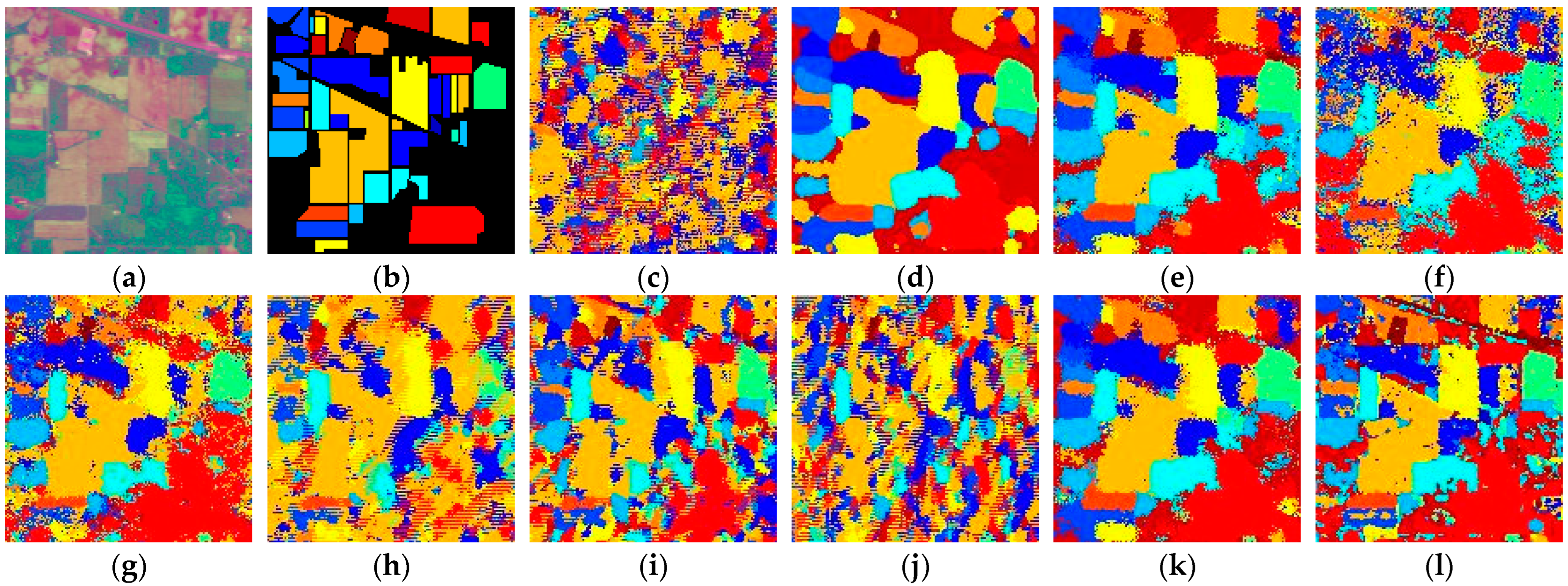
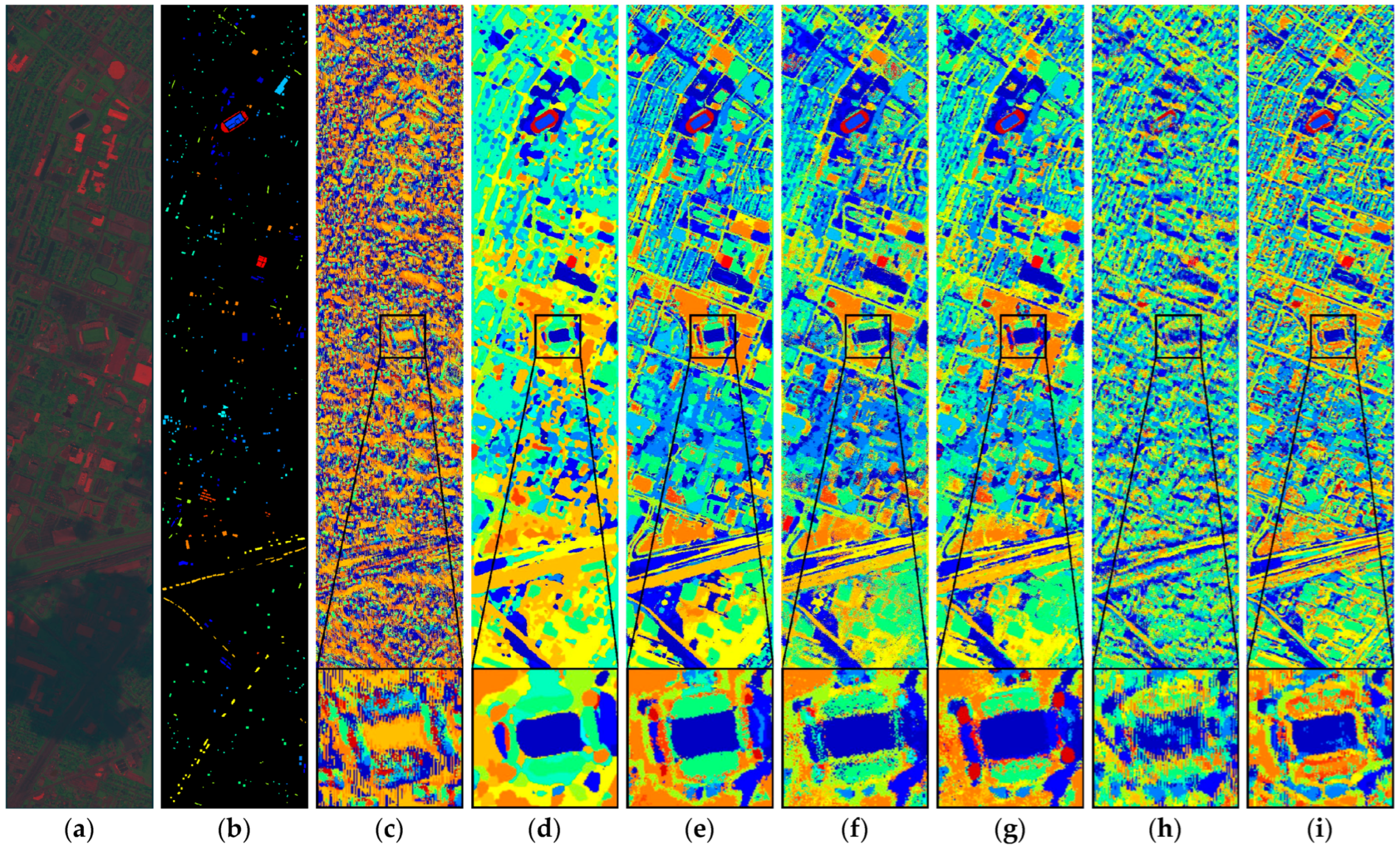
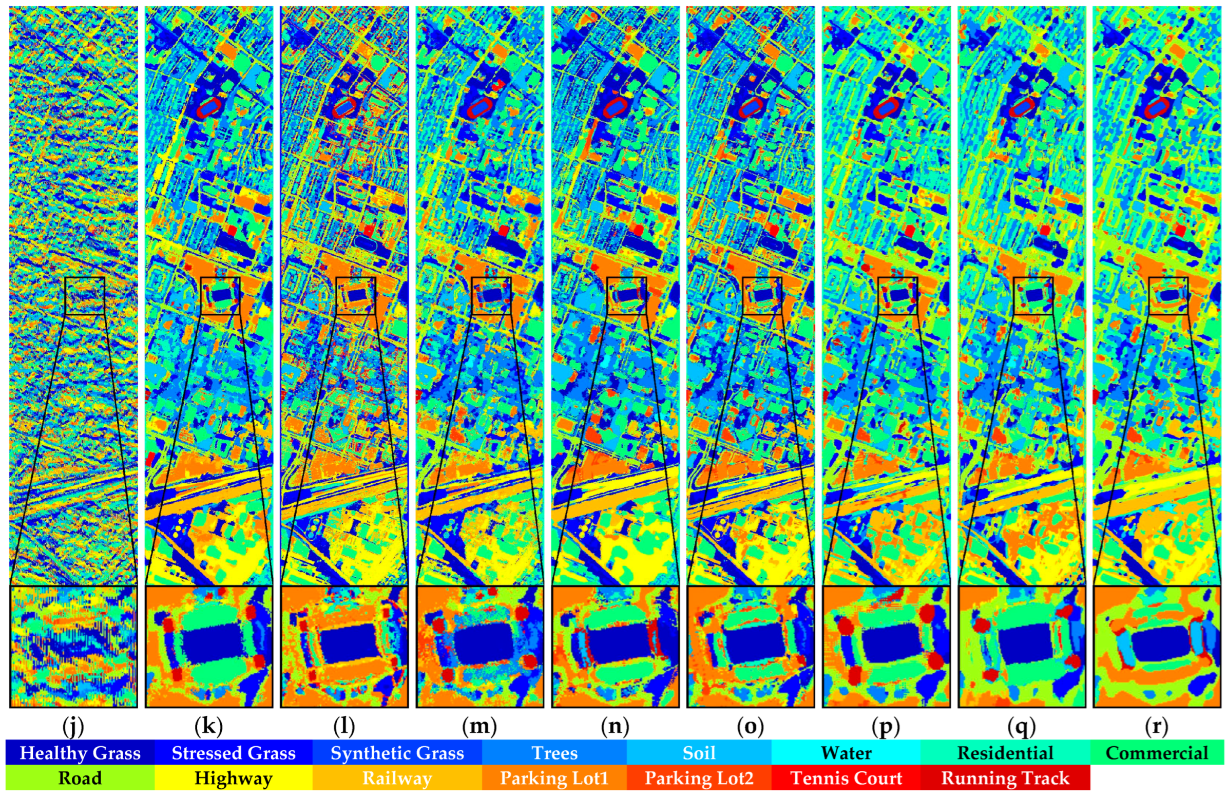
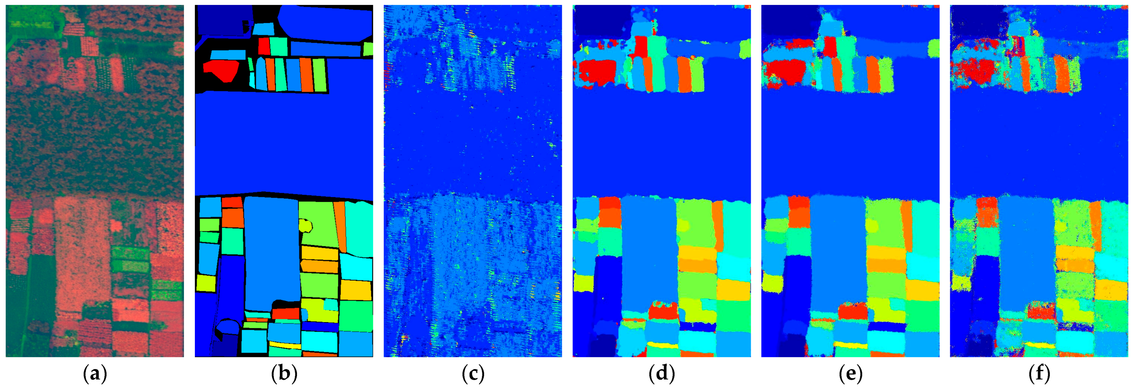
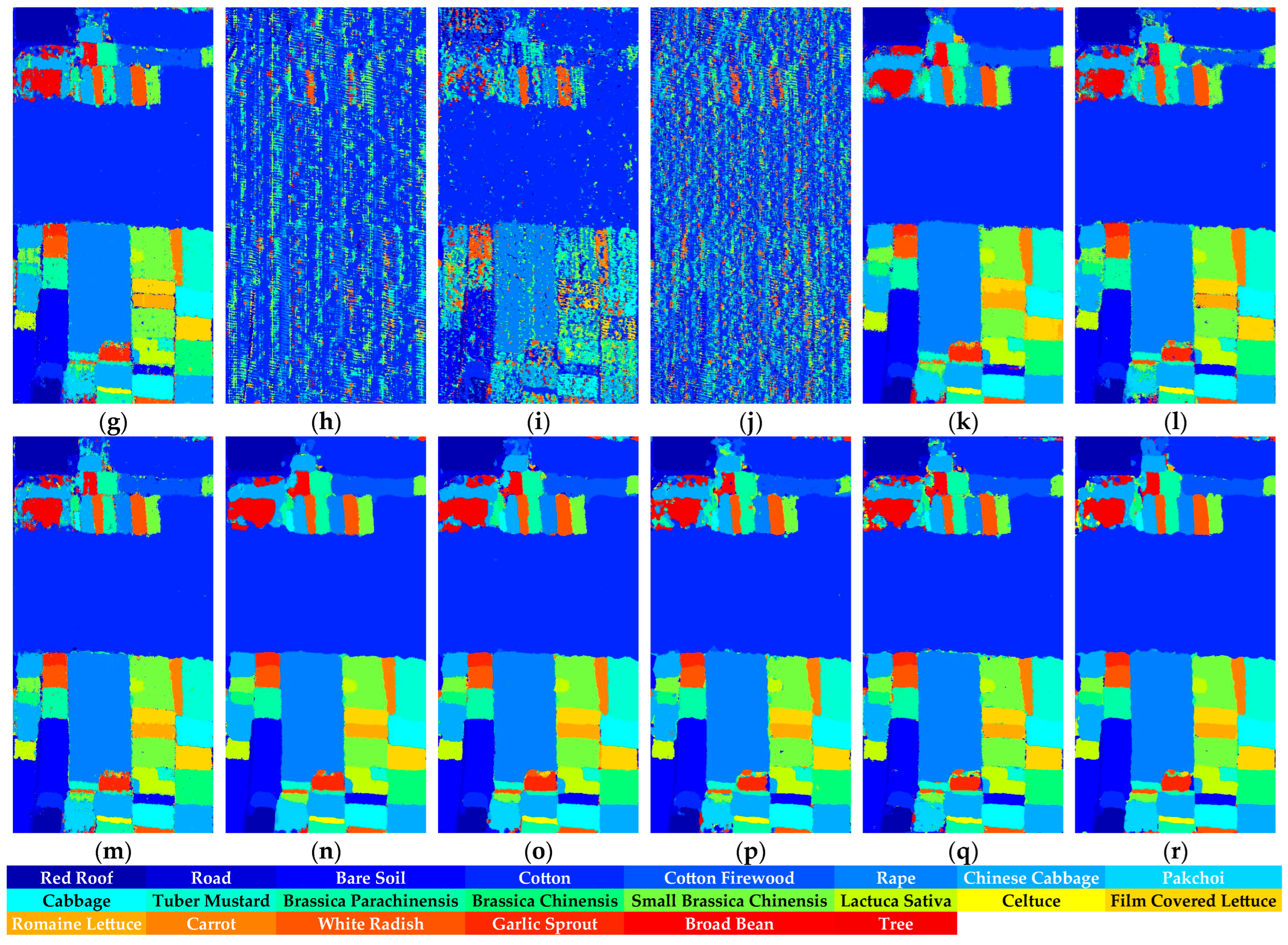
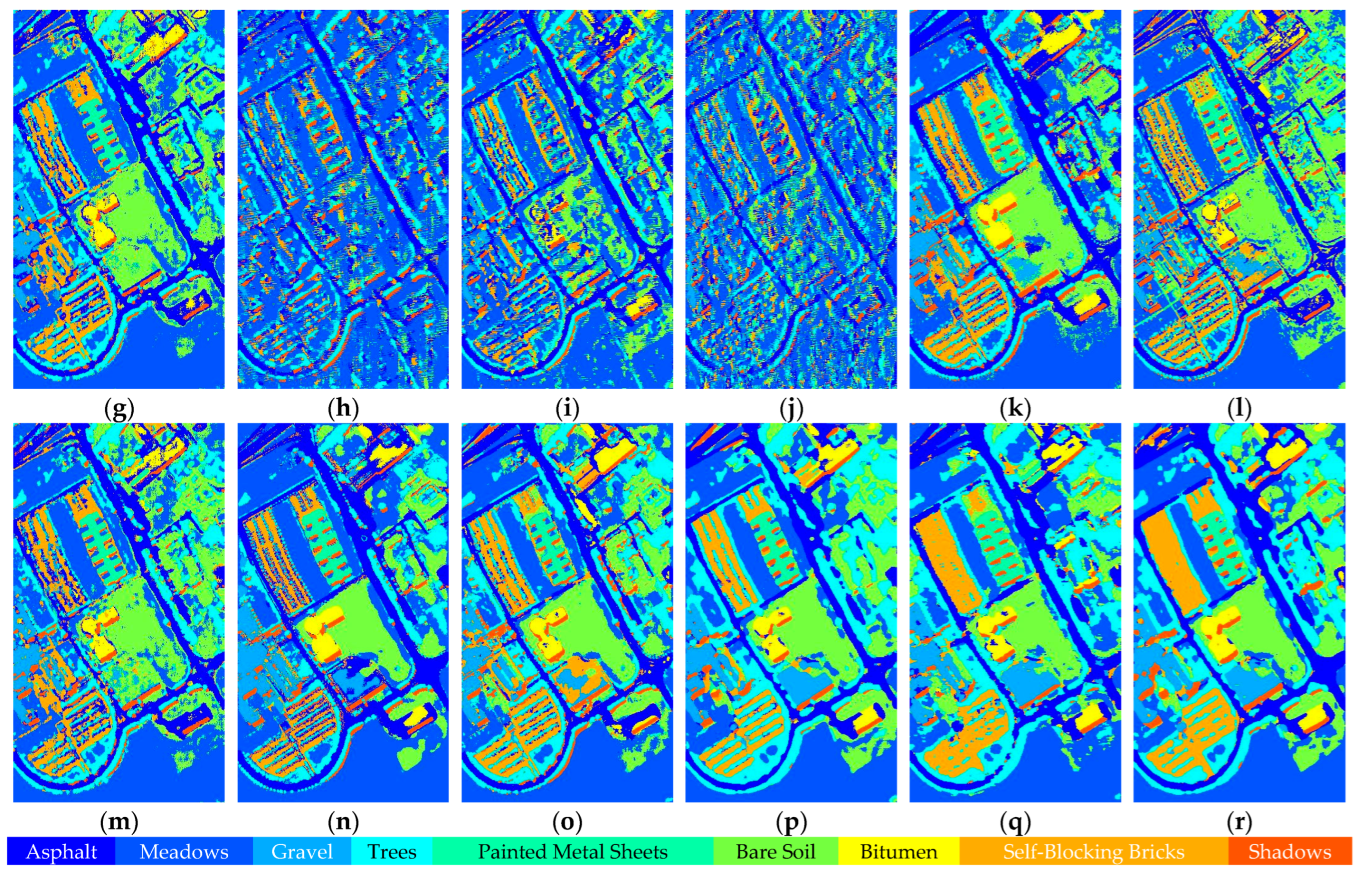
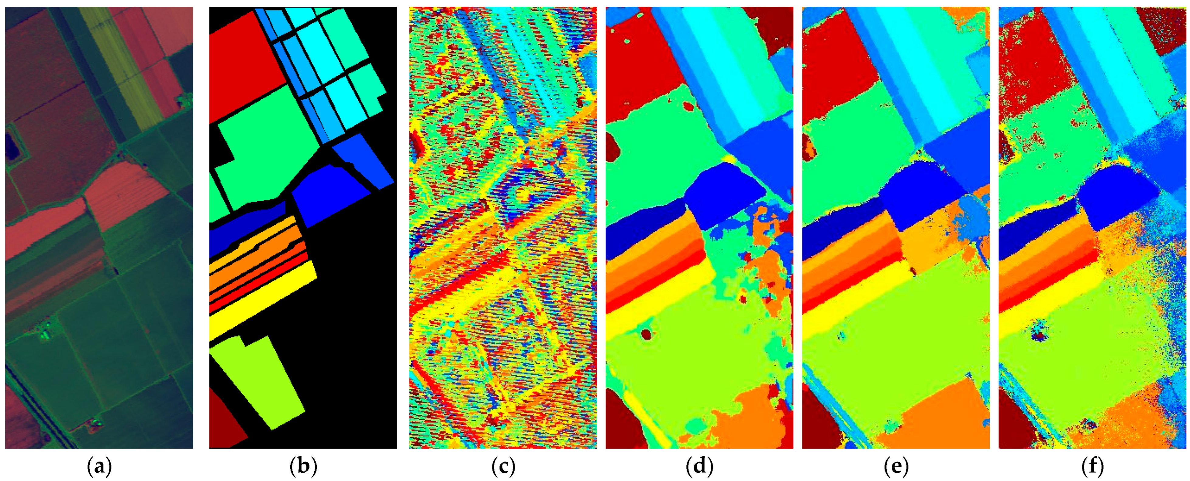
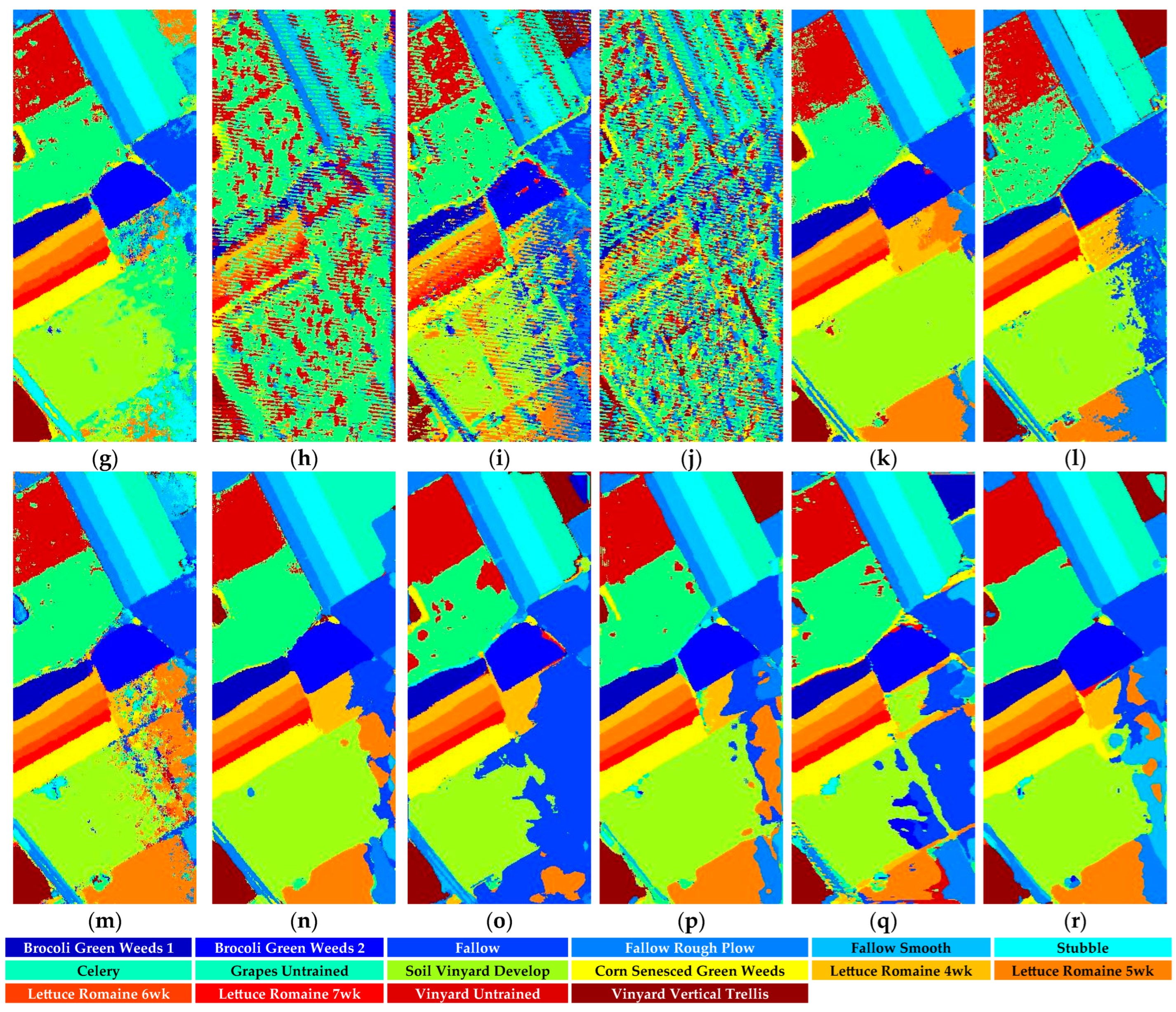
To further evaluate spatial coherence and boundary retention of the classification results obtained by different networks, this section conducts full-scene classification experiments. We use the classification network to predict the class label of all pixels. The full-scene classification results obtained by different networks from five HSI datasets are shown in Figure 14, Figure 15, Figure 16, Figure 17 and Figure 18. The full-scene classification performance obtained by different networks from five HSI datasets is shown in

Table 23. Full-scene classification performance obtained by S3ARN, PMCN, S3GAN, ViT, SFormer, HFormer, MHCFormer, and D2S2BoT from five public HSI datasets. The optimal results and suboptimal results are in red and blue, respectively.

Datasets	Metrics	S3ARN	PMCN	S3GAN	ViT	SFormer	HFormer	MHCFormer	D2S2BoT
Indian	MI (%)	36.87 ± 5.30	89.33 ± 1.18	79.99 ± 0.71	50.83 ± 6.78	62.02 ± 4.52	45.74 ± 3.47	67.55 ± 1.78	50.63 ± 4.53
	BF1 (%)	63.39 ± 2.25	98.26 ± 0.48	97.90 ± 1.00	78.23 ± 3.73	83.05 ± 3.40	66.68 ± 1.34	85.37 ± 0.83	68.45 ± 0.62
	SSIM (%)	53.93 ± 5.62	88.92 ± 0.63	88.97 ± 0.90	66.35 ± 2.47	72.35 ± 2.85	68.99 ± 1.51	73.47 ± 0.72	58.72 ± 0.77
Houston	MI (%)	44.51 ± 5.21	91.00 ± 0.49	81.41 ± 0.97	65.50 ± 5.05	73.69 ± 3.51	49.62 ± 4.41	66.18 ± 1.13	60.81 ± 1.55
	BF1 (%)	95.86 ± 1.34	96.74 ± 0.23	96.98 ± 0.12	96.78 ± 0.31	97.04 ± 0.05	94.37 ± 1.49	96.81 ± 0.36	95.63 ± 0.23
	SSIM (%)	94.40 ± 1.43	98.34 ± 0.05	98.56 ± 0.04	98.08 ± 0.14	98.20 ± 0.10	97.24 ± 0.12	98.05 ± 0.07	96.90 ± 0.14
HongHu	MI (%)	61.16 ± 8.24	96.97 ± 0.22	94.98 ± 0.49	83.96 ± 1.13	90.51 ± 0.74	52.68 ± 2.21	66.03 ± 3.14	45.44 ± 2.05
	BF1 (%)	26.40 ± 5.74	97.32 ± 0.08	95.36 ± 1.39	53.36 ± 3.36	77.59 ± 2.58	20.60 ± 1.38	26.49 ± 0.70	16.32 ± 2.22
	SSIM (%)	26.62 ± 10.1	91.42 ± 0.02	90.12 ± 0.75	66.89 ± 2.24	78.95 ± 1.31	24.25 ± 9.36	37.17 ± 3.70	13.52 ± 0.21
PaviaU	MI (%)	51.99 ± 2.18	90.02 ± 0.61	77.37 ± 1.79	63.28 ± 1.97	69.59 ± 2.10	53.99 ± 2.28	66.56 ± 0.73	52.35 ± 1.86
	BF1 (%)	64.96 ± 3.38	84.61 ± 0.30	85.21 ± 0.16	85.57 ± 1.29	87.03 ± 0.78	72.66 ± 1.13	77.30 ± 0.75	66.68 ± 0.82
	SSIM (%)	69.03 ± 0.86	84.73 ± 0.41	85.56 ± 0.08	81.64 ± 0.78	83.40 ± 0.20	71.59 ± 0.60	75.47 ± 0.89	69.54 ± 0.34
Salinas	MI (%)	51.64 ± 5.72	96.05 ± 0.28	94.54 ± 0.39	82.53 ± 1.54	89.10 ± 3.18	51.58 ± 1.16	71.83 ± 1.83	50.82 ± 3.08
	BF1 (%)	29.40 ± 1.59	97.11 ± 0.14	96.48 ± 0.60	81.43 ± 1.99	89.38 ± 0.52	33.26 ± 1.14	49.25 ± 1.73	27.54 ± 0.63
	SSIM (%)	55.38 ± 2.14	94.19 ± 0.22	93.44 ± 0.63	85.22 ± 1.63	88.79 ± 0.47	58.38 ± 0.54	65.33 ± 1.91	54.65 ± 0.61

and

Table 24. Full-scene classification performance obtained by SQSFormer, EATN, CFormer, SSACFormer, CPFormer, DSFormer, LGDRNet, and CPMFFormer from five public HSI datasets. The optimal results and suboptimal results are in red and blue, respectively.

Datasets	Metrics	SQSFormer	EATN	CFormer	SSACFormer	CPFormer	DSFormer	LGDRNet	CPMFFormer
Indian	MI (%)	78.65 ± 1.22	76.89 ± 0.84	72.78 ± 2.79	83.54 ± 2.75	80.96 ± 2.69	88.53 ± 0.83	87.34 ± 1.13	91.78 ± 0.95
	BF1 (%)	96.21 ± 0.76	91.00 ± 0.66	93.93 ± 1.62	97.19 ± 1.15	97.63 ± 0.64	97.96 ± 0.69	98.18 ± 0.36	99.17 ± 0.10
	SSIM (%)	86.64 ± 0.73	81.74 ± 0.95	82.91 ± 1.54	88.54 ± 1.49	87.97 ± 0.96	89.31 ± 0.87	87.66 ± 0.78	92.73 ± 0.39
Houston	MI (%)	82.25 ± 0.84	73.20 ± 1.81	79.67 ± 0.75	83.48 ± 1.41	79.01 ± 2.47	85.40 ± 0.88	89.22 ± 1.30	91.31 ± 0.44
	BF1 (%)	96.77 ± 0.23	97.02 ± 0.13	96.99 ± 0.06	96.85 ± 0.32	97.04 ± 0.41	96.90 ± 0.15	97.09 ± 0.20	97.12 ± 0.17
	SSIM (%)	98.44 ± 0.06	98.47 ± 0.05	98.46 ± 0.04	98.43 ± 0.07	98.44 ± 0.08	98.48 ± 0.05	98.44 ± 0.11	98.62 ± 0.05
HongHu	MI (%)	92.67 ± 0.46	91.18 ± 0.37	92.82 ± 0.41	97.19 ± 0.26	96.57 ± 0.29	96.24 ± 0.08	96.29 ± 0.14	97.66 ± 0.11
	BF1 (%)	87.03 ± 1.41	83.09 ± 1.42	88.93 ± 2.02	98.24 ± 0.18	97.06 ± 0.70	93.93 ± 0.23	95.92 ± 0.49	98.53 ± 0.05
	SSIM (%)	86.49 ± 0.63	83.99 ± 0.63	84.85 ± 1.16	92.13 ± 0.16	91.22 ± 0.46	89.67 ± 0.12	90.58 ± 0.36	92.54 ± 0.08
PaviaU	MI (%)	74.94 ± 0.61	70.91 ± 0.63	72.42 ± 0.68	77.70 ± 2.27	82.00 ± 1.86	88.69 ± 0.39	87.88 ± 0.62	91.80 ± 0.25
	BF1 (%)	85.33 ± 0.59	85.50 ± 0.53	86.46 ± 0.61	85.80 ± 0.32	85.15 ± 1.25	85.27 ± 0.25	85.45 ± 0.45	86.84 ± 0.16
	SSIM (%)	85.02 ± 0.26	83.49 ± 0.19	84.29 ± 0.30	85.43 ± 0.25	85.29 ± 0.90	85.52 ± 0.08	84.86 ± 0.40	85.98 ± 0.13
Salinas	MI (%)	93.37 ± 0.64	90.52 ± 0.87	89.31 ± 1.85	96.41 ± 0.22	94.83 ± 0.56	95.84 ± 0.23	95.29 ± 0.59	96.67 ± 0.11
	BF1 (%)	87.15 ± 1.74	80.37 ± 2.04	94.15 ± 0.53	96.73 ± 0.92	96.47 ± 1.17	94.75 ± 0.96	94.48 ± 1.04	97.99 ± 0.20
	SSIM (%)	88.99 ± 0.36	84.15 ± 0.79	91.28 ± 0.43	93.95 ± 0.6	93.63 ± 1.06	92.57 ± 0.	92.26 ± 0.40	95.19 ± 0.17

.

According to the experimental results, it can be seen that the full-scene classification results generated by S3ARN, HFormer, MHCFormer, and D2S2BoT are significantly worse than those of other classification networks. Although they achieve a better classification performance in Section 4.4, they perform poorly in the full-scene classification experiment. This is mainly because these models only consider the spectral–spatial features within the sample patch, while ignoring the spatial distribution differences between adjacent ground objects. Although these models can extract multiscale spatial features to better characterize complex spatial relationships and model the diverse spatial distribution patterns presented by ground objects, their limitations in the multiscale features fusion strategy may lead to information confusion and semantic conflicts. This reduces the spatial features representational capability. These networks lack the center feature calibration mechanism. This makes it difficult for them to suppress interference information and causes them to be prone to generating misclassified pixels.

In contrast, other classification networks can generate smoother full-scene classification results. Especially for the center attention networks, they perform better than other networks. This is mainly because these networks can calculate dependencies between the center pixel and its neighboring pixels. This helps them to dynamically select the valuable neighboring spectral–spatial features and effectively prevent the transmission and amplification of interference information. For the ground object boundaries, the center attention mechanism can accurately capture characteristic differences between the center pixels and their surrounding regions. This avoids class leakage and boundary blurring. These advantages enable the center attention networks to maintain stable and high-precision classification performance in full-scene classification tasks.

Compared with comparison networks, CPMFFormer can capture subtle spectral differences between ground objects. Moreover, it can hierarchically enhance discriminative spatial features at different scales. This is beneficial for reducing misclassified pixels and ensuring spatial coherence in the full-scene classification. Furthermore, CPMFFormer achieves a smooth semantic transition through the progressive multiscale fusion strategy. It can better model spatial correlations and enhance the spatial feature representational capability. As shown in Table 23 and Table 24, CPMFFormer achieved the best full-scene classification performance from most HSI datasets. Only its BF1 from the PaviaU dataset is slightly worse than that of SFormer. This is mainly because the PaviaU dataset contains a large amount of detailed information, which results in the input patch containing more interference pixels. This makes it easy for the classification network to learn incorrect spatial features. SFormer focuses more on spectral long-range dependence and has a relatively low dependence on spatial neighboring information. Its classification result is less affected by interference pixels, so it has better boundary retention performance. However, this also makes SFormer prone to generating non-smooth classification results. Therefore, SFormer has a lower spatial coherence on the PaviaU dataset.

4.6. Network Stability Evaluation

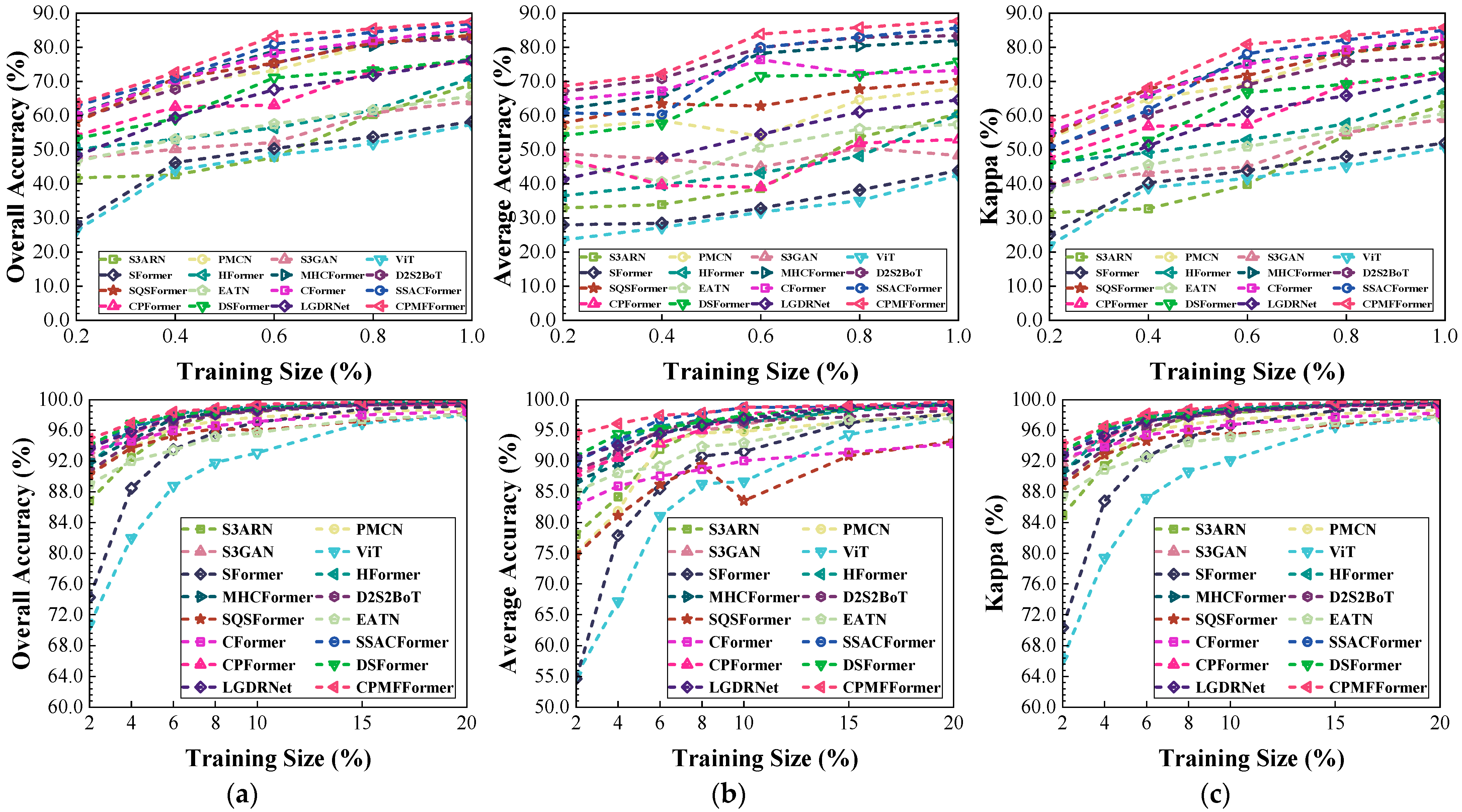
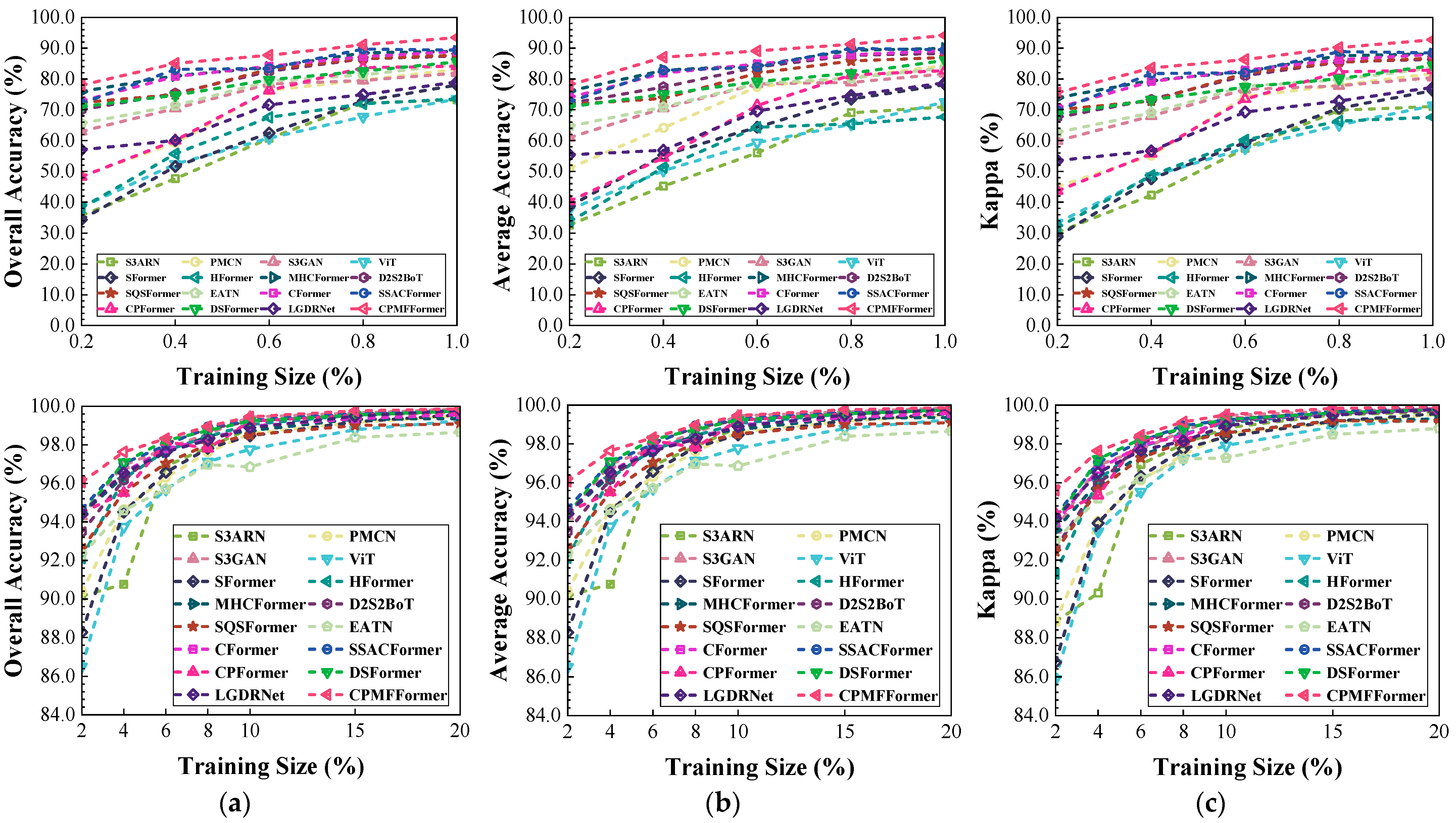
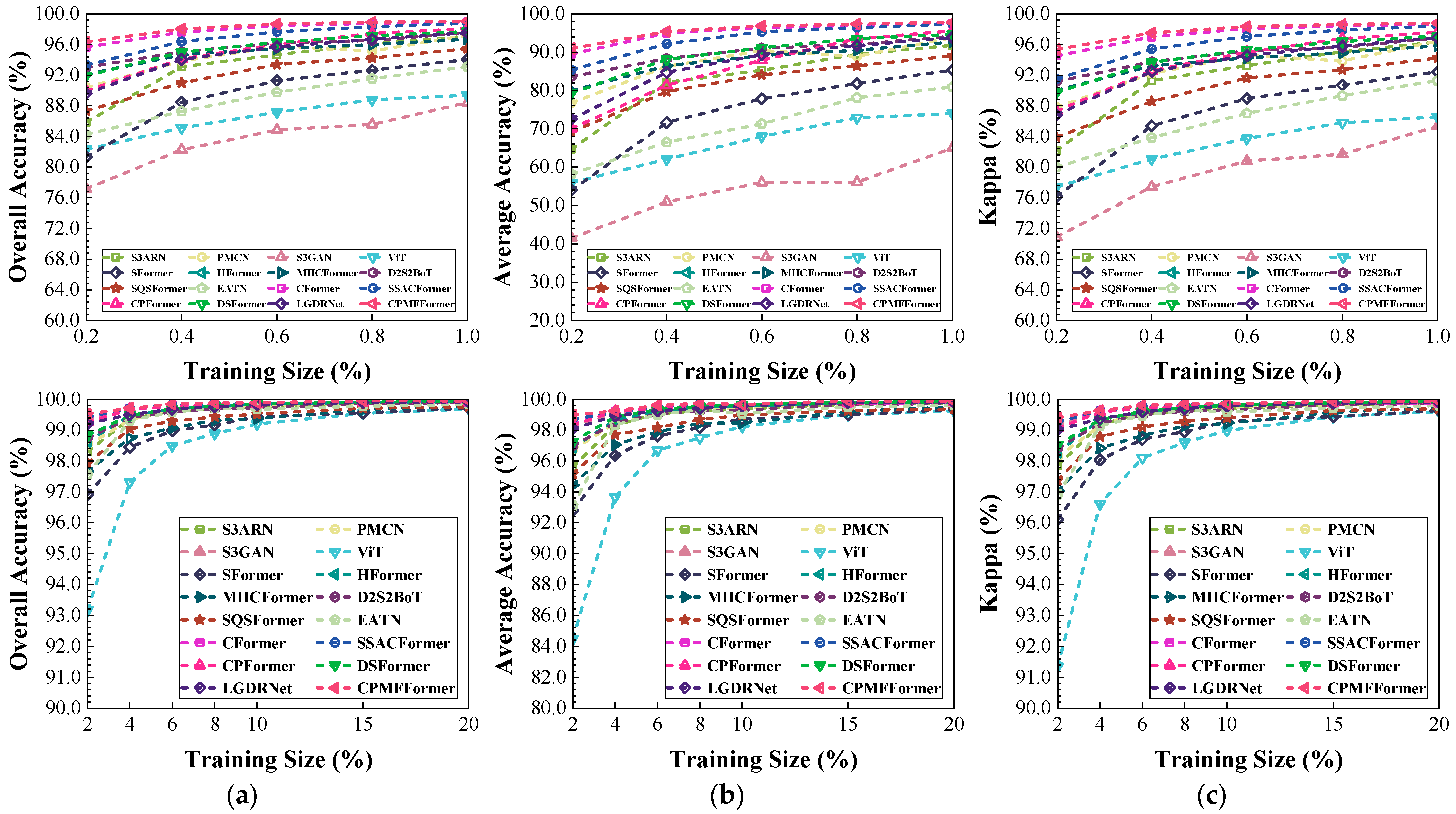
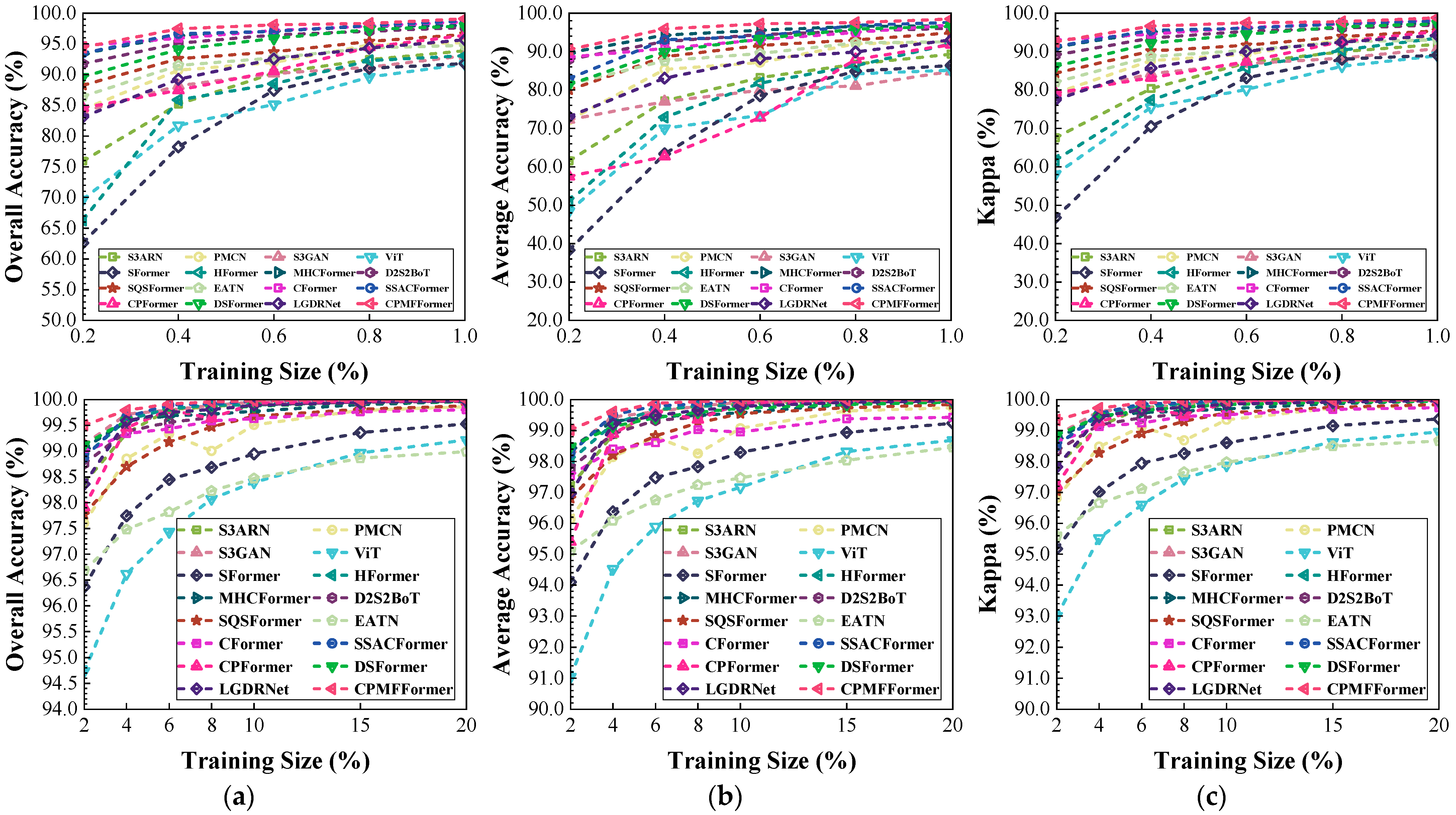
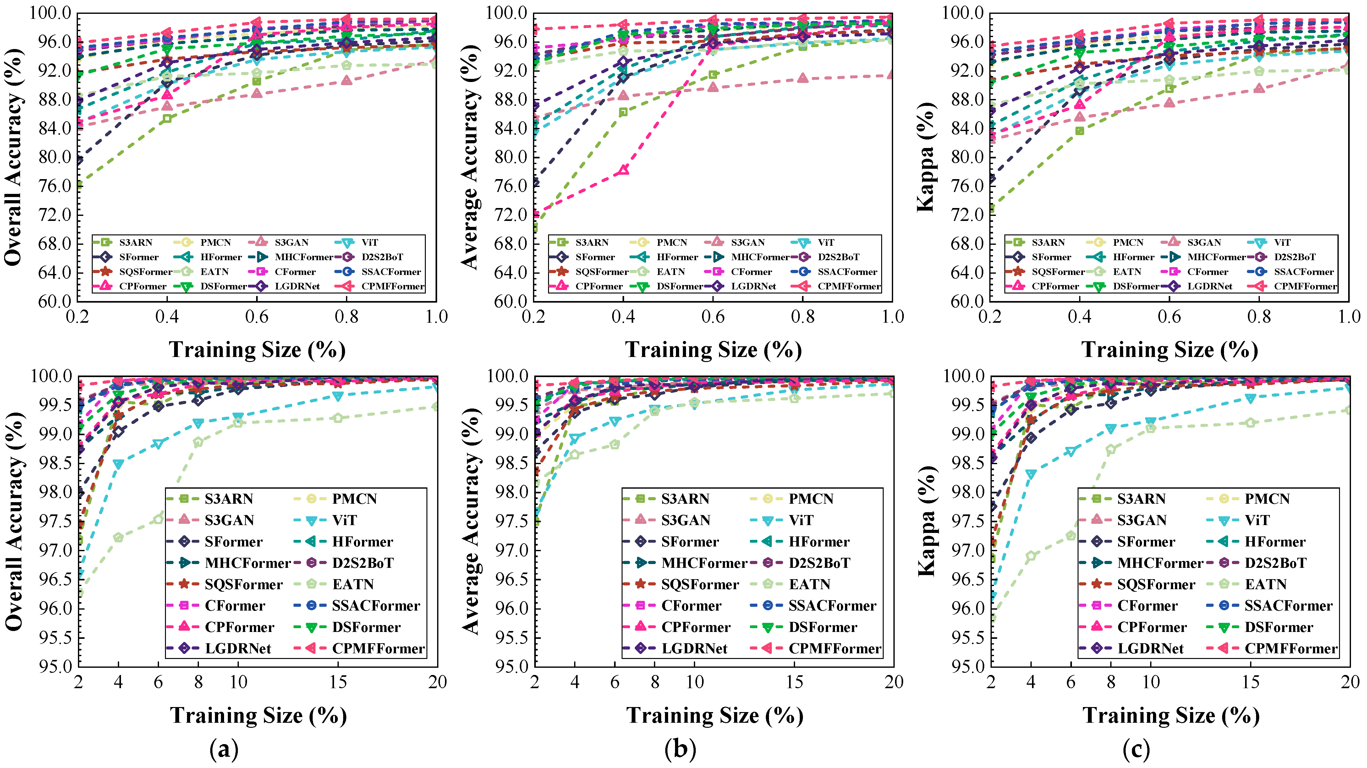
Network stability is an important indicator for evaluating classification performance. It ensures that the classification network can operate reliably and efficiently in practical applications. To validate the stability of CPMFFormer, this section sets the training sample sizes to 0.2%, 0.4%, 0.6%, 0.8%, 1%, 2%, 4%, 6%, 8%, 10%, 15%, and 20% of all label samples to analyze the performance changes in different networks. The experimental results obtained by different networks with different training sample sizes from five public HSI datasets are shown in Figure 19, Figure 20, Figure 21, Figure 22 and Figure 23.

It can be seen that under the impact of different training sample sizes, the performance of most classification networks on all HSI datasets generally shows a reasonable trend, that is, as the training sample size increases, their classification performance gradually improves. When there are sufficient training samples, most networks almost achieve optimal classification performance on five HSI datasets.

The experimental results show that compared with other classification networks, the performance curve of CPMFFormer converges faster in five HSI datasets. This demonstrates that CPMFFormer exhibits stronger stability. Furthermore, it is worth noting that at any training sample size, CPMFFormer performs better than other classification networks on all HSI datasets. Especially when there are fewer training samples (such as when the training sample size is less than 1%), the advantage of CPMFFormer in classification performance is more obvious. The above analyses indicate that the proposed classification network has better generalization performance and practicality.

4.7. Network Complexity and Inference Efficiency

Computational complexity affects training efficiency and resource consumption of the classification network. As shown in

Table 25. Computational complexity of S3ARN, PMCN, S3GAN, ViT, SFormer, HFormer, MHCFormer, and D2S2BoT.

Dataset	Metrics	S3ARN	PMCN	S3GAN	ViT	SFormer	HFormer	MHCFormer	D2S2BoT
Indian	Params (M)	8.1104	0.2288	0.0866	0.0954	0.3426	3.3918	0.4090	0.4560
	FLOPs (G)	1.0752	0.9697	2.6063	0.0381	0.0708	0.6258	0.0569	0.3742
	Training Time(s)	67.03	130.72	366.14	23.87	26.40	59.59	40.95	37.07
	Testing Time (s)	3.31	7.06	12.94	1.22	1.61	3.68	2.10	2.09
Houston	Params (M)	5.2644	0.1936	0.0599	0.0954	0.2262	2.8042	0.4089	0.4559
	FLOPs (G)	0.5612	0.7040	2.4428	0.0275	0.0448	0.3628	0.0569	0.3742
	Training Time(s)	82.79	137.26	461.06	26.50	34.21	76.08	57.44	51.93
	Testing Time (s)	4.41	7.28	17.70	1.75	2.25	4.62	3.36	3.04
HongHu	Params (M)	12.3283	0.2730	0.1259	0.0958	0.5415	4.4071	0.4094	0.4567
	FLOPs (G)	1.9505	1.3020	5.7876	0.0514	0.1100	1.0737	0.0569	0.3742
	Training Time(s)	2675.17	7416.70	31,776.6	900.77	1006.45	1919.27	1338.53	1281.81
	Testing Time (s)	132.11	360.21	1032.46	50.36	72.69	125.23	80.79	76.82
PaviaU	Params (M)	3.4804	0.1675	0.0465	0.0950	0.1644	2.4754	0.4085	0.4552
	FLOPs (G)	0.2912	0.5094	2.3408	0.0197	0.0289	0.2239	0.0569	0.3742
	Training Time(s)	204.73	297.33	1464.42	70.12	93.51	193.33	147.42	140.20
	Testing Time (s)	12.30	16.27	49.14	4.72	6.02	12.06	8.87	8.61
Salinas	Params (M)	8.3308	0.2313	0.0878	0.0954	0.3524	3.4407	0.4090	0.4560
	FLOPs (G)	1.1182	0.9887	2.6163	0.0389	0.0729	0.6478	0.0569	0.3742
	Training Time(s)	332.57	735.30	2063.5	93.17	147.86	270.07	198.95	179.84
	Testing Time (s)	16.51	35.26	68.83	6.52	9.23	18.49	10.76	16.51

and

Table 26. Computational complexity of SQSFormer, EATN, CFormer, SSACFormer, CPFormer, DSFormer, LGDRNet, and CPMFFormer.

Dataset	Metrics	SQSFormer	EATN	CFormer	SSACFormer	CPFormer	DSFormer	LGDRNet	CPMFFormer
Indian	Params (M)	0.2585	0.3914	0.6156	0.7060	0.6142	0.5939	0.3550	0.6688
	FLOPs (G)	0.0839	0.0949	0.1235	0.2319	0.2592	0.0421	2.8689	0.1495
	Training Time(s)	9.53	129.32	67.61	182.40	116.98	47.19	38.88	33.04
	Testing Time (s)	0.76	3.01	6.54	5.57	10.05	2.66	1.58	2.53
Houston	Params (M)	0.1490	0.3168	0.6118	0.3799	0.3202	0.5938	0.3549	0.2065
	FLOPs (G)	0.0469	0.0769	0.1219	0.2525	0.1353	0.0421	3.1857	0.0467
	Training Time(s)	9.50	201.38	98.34	262.50	131.67	55.93	41.70	42.89
	Testing Time (s)	0.55	4.05	7.53	9.65	11.62	3.94	2.40	3.33
HongHu	Params (M)	0.1614	0.5025	0.6217	1.2527	1.1136	0.5947	0.3553	0.2855
	FLOPs (G)	0.0508	0.1701	0.1255	0.7171	0.4692	0.0421	2.9004	0.0898
	Training Time(s)	214.56	1358.34	1041.4	9239.8	2074.2	1464.4	1578.6	1557.54
	Testing Time (s)	15.61	155.57	359.00	254.58	450.38	96.87	73.89	103.06
PaviaU	Params (M)	0.1597	0.2699	0.6076	0.2035	0.1597	0.5930	0.3546	0.5526
	FLOPs (G)	0.0508	0.0656	0.1207	0.1125	0.0508	0.0421	2.2926	0.1224
	Training Time(s)	23.75	192.68	114.54	332.19	247.22	147.11	133.71	149.93
	Testing Time (s)	1.72	7.53	14.87	17.59	24.36	9.72	6.62	9.69
Salinas	Params (M)	0.1606	0.3972	0.6159	0.7331	0.6389	0.5939	0.3550	0.2434
	FLOPs (G)	0.1324	0.0963	0.1236	0.3347	0.2025	0.0421	2.3463	0.0769
	Training Time(s)	93.21	225.69	167.73	539.63	339.52	201.26	177.06	202.99
	Testing Time (s)	35.26	13.63	31.36	29.27	39.40	13.36	8.55	10.76

, this section counts the trainable parameters, computational cost, training time, and testing time of different classification networks on five HSI datasets. The trainable parameters are in millions ($M$), the computational cost is in $GFLOPs$, and the training and testing times are in seconds ($s$).

As shown in Table 25 and Table 26, although this paper designs multiple modules to improve the feature representation capability, the computational complexity of CPMFFormer is not the highest. This is due to our optimization of the network framework. For example, this paper introduces the bottleneck structure into CRCM and CSFBT. This reduces the feature channels’ dimension. Moreover, when extracting features at different scales using group convolution, this paper adaptively allocates the feature channels’ dimension in each group based on the convolutional kernel size. These designs reduce the computational complexity of CPMFFormer. Furthermore, it is undeniable that some classification networks have smaller computational complexity than our network. However, it is worth noting that the difference in computational complexity between CPMFFormer and these classification networks is small, but the classification performance of CPMFFormer is much better than theirs. This demonstrates that CPMFFormer achieves a good compromise between computational complexity and classification performance.

4.8. Ablation Study

To analyze the impact of some important contributions in CPMFFormer on classification performance, this section carries out the ablation study from three aspects, including the ablation study on the overall framework, the ablation study on the spectral weighting mechanism, and the ablation study on the attention mechanism.

Ablation Study on the Overall Framework: CPMFFormer constructs three main modules to enhance the feature representation capability and improve classification performance, including CSWM, CRCM, and CSFBT. To validate their effectiveness, this section removes CSWM, CRCM, and CSFBT to carry out experiments.

As shown in Figure 24, after removing each module, the classification performance of CPMFFormer decreases to varying degrees. This shows that these modules are effective in improving classification performance. Specifically, after removing CSWM, CPMFFormer focuses more on extracting multiscale spatial features and ignores spectral features. This makes it difficult for CPMFFormer to reveal subtle differences in the spectral radiation characteristics of different ground objects. Moreover, it is worth noting that after removing CRCM, CSFBT used for multiscale features’ fusion is also removed because there is no multiscale feature extraction. In this case, CPMFFormer only depends on CSWM to extract class-discriminative spectral features but cannot obtain high-level spatial semantic features to model complex spatial relationships. Therefore, the classification performance after removing CRCM is significantly worse than other experiments. After removing CSFBT, CPMFFormer mainly uses the output features of the last CRCM to predict the class probabilities. This makes CPMFFormer neglect complementary features from other scales and reduce the feature representation capability. Removing both CSWM and CSFBT causes CPMFFormer to lack spectral awareness capability and have difficulty in capturing cross-scale complementary information. The classification performance is significantly worse than that obtained after separately removing CSWM and CSFBT. This demonstrates the synergistic and promoting effects between different modules.

This paper builds a progressive multiscale fusion strategy to promote the effective collaboration between different scale features. This achieves a smooth semantic transition by gradually fusing adjacent scale features, while avoiding information confusion and semantic conflict between features with large-scale differences. As shown in Figure 4, CPMFFormer uses six CSFBTs to enhance scale-specific information. To validate their effectiveness, this section uses the progressive multiscale fusion strategy to fuse features at different scales shown in Figure 2. The activation response heatmaps obtained by different CSFBTs on the PaviaU dataset are shown in Figure 25. The experimental results show that as the fusion level increases, the progressive multiscale fusion strategy gradually integrates semantic information specific to different scales into the fusion features. As shown in Figure 25f, the fusion features obtained by CSFBT-6 not only retain the larger activation response in small-scale features to the Trees class (red box) but also retain the larger activation response in large-scale features to the Painted Metal Sheets class (white box).

To comprehensively analyze the effectiveness of the progressive multiscale fusion strategy, this paper visualizes the activation responses obtained by current multiscale fusion methods, including concatenation, element-wise addition, and attention method in the literature [35]. As shown in Figure 26, it is difficult for concatenation and element-wise additions to effectively integrate complementary information at different scales. In contrast, the attention method can enhance the activation responses to the Trees and Painted Metal Sheets classes to a certain extent. However, compared with the fusion features obtained by the progressive multiscale fusion strategy, the fusion features obtained by the attention method have smaller activation responses to different ground objects. This reduces the features representation capability and affects classification performance.

Ablation Study on the Spectral Weighting Mechanism: To obtain the class-specific spectral weights, CSWM introduces an aggregation operation and a class consistency loss into spectral weight learning (SWL). To validate its effectiveness, we remove the aggregation operation and class consistency loss in CSWM and only use SWL to learn spectral weights. As shown in Figure 27, after removing the aggregation operation and class consistency loss function, the classification performance of CPMFFormer decreases. This is mainly because spectral variability causes the spectral distribution characteristics of different ground objects to be approximately the same. SWL only relies on spectral information to learn spectral weights. This makes it difficult for CPMFFormer to distinguish samples with similar spectral characteristics, but which not belong to the same class.

As shown in Figure 1, the spectral distribution characteristics of the Corn-Notill class, Corn-Mintill class, and Corn class in the Indian dataset overlap with each other. To further validate the effectiveness of CSWM, this section visualizes the average spectral weights learned by SWL and CSWM for the Corn-Notill class, Corn-Mintill class, and Corn class, as shown in Figure 28. It can be seen from the visualization results that since SWL lacks class information, the average spectral weights learned by SWL for the Corn-Notill class, Corn-Mintill class, and Corn class are basically the same. This makes it difficult for SWL to obtain discriminative spectral features that are beneficial for characterizing different ground objects with similar spectra. In contrast, the average spectral weights learned by CSWM for the Corn-Notill class, Corn-Mintill class, and Corn class have obvious differences. This enhances class-discriminative spectral features and increases inter-class spectral differences. This enables the proposed classification network to effectively deal with inter-class spectral overlap and accurately distinguish samples with similar spectra, but which belong to different classes, thereby improving classification performance.

Ablation Study on the Attention Mechanism: This paper designs three different attention mechanisms to enhance the feature representation capability, including CFCL, CFEB, and MHCSD2A. MHCSD2A is composed of a cross-scale spatial attention (CSSA) and a cross-scale channel attention (CSCA). To validate their effectiveness, this paper removes different attention mechanisms to carry out experiments. As shown in

Table 27. Impact of different attention mechanisms on classification performance. The best results are in red.

Dataset	Metrics	Without CFCL	Without CFEB	Without CSSA	Without CSCA	Without MHCSD2A	CPMFFormer
Indian	OA (%)	93.84 ± 0.91	93.96 ± 1.03	93.54 ± 1.49	93.05 ± 1.00	92.61 ± 2.17	94.85 ± 0.69
	AA (%)	93.14 ± 1.34	93.69 ± 2.50	93.66 ± 4.35	93.03 ± 2.09	91.17 ± 3.14	94.35 ± 0.61
	$\kappa$ (%)	92.97 ± 0.99	93.11 ± 1.16	92.63 ± 1.69	92.07 ± 1.13	91.59 ± 2.45	94.13 ± 0.80
Houston	OA (%)	92.95 ± 3.12	94.63 ± 1.01	94.99 ± 0.54	94.49 ± 1.18	93.73 ± 4.11	95.93 ± 0.36
	AA (%)	93.44 ± 2.82	95.07 ± 0.88	95.26 ± 0.74	94.75 ± 1.14	93.99 ± 3.84	96.06 ± 0.26
	$\kappa$ (%)	92.38 ± 3.38	94.20 ± 1.10	94.59 ± 0.59	94.05 ± 1.28	93.22 ± 4.45	95.61 ± 0.39
HongHu	OA (%)	99.35 ± 0.11	99.36 ± 0.08	99.34 ± 0.04	99.45 ± 0.04	99.18 ± 0.04	99.53 ± 0.03
	AA (%)	98.47 ± 0.65	98.37 ± 0.15	98.46 ± 0.13	98.62 ± 0.13	98.37 ± 0.18	98.99 ± 0.10
	$\kappa$ (%)	99.18 ± 0.14	99.20 ± 0.10	99.17 ± 0.05	99.31 ± 0.05	99.02 ± 0.05	99.41 ± 0.04
PaviaU	OA (%)	99.26 ± 0.13	99.31 ± 0.21	99.36 ± 0.21	99.27 ± 0.17	99.13 ± 0.25	99.50 ± 0.06
	AA (%)	98.64 ± 0.25	98.72 ± 0.41	98.78 ± 0.36	98.68 ± 0.29	98.20 ± 0.56	99.02 ± 0.10
	$\kappa$ (%)	99.01 ± 0.17	99.08 ± 0.28	99.15 ± 0.28	99.04 ± 0.22	98.84 ± 0.33	99.34 ± 0.08
Salinas	OA (%)	99.75 ± 0.07	99.69 ± 0.08	99.68 ± 0.10	99.65 ± 0.08	99.37 ± 0.20	99.84 ± 0.06
	AA (%)	99.69 ± 0.08	99.65 ± 0.09	99.61 ± 0.11	99.57 ± 0.09	99.52 ± 0.09	99.84 ± 0.05
	$\kappa$ (%)	99.72 ± 0.09	99.66 ± 0.08	99.65 ± 0.11	99.62 ± 0.09	99.19 ± 0.22	99.82 ± 0.07

, after removing each attention mechanism, the classification performance of CPMFFormer decreases to varying degrees. This shows that these attention mechanisms are effective in enhancing the feature representation capability and improving classification performance.

4.9. Expandability Analysis

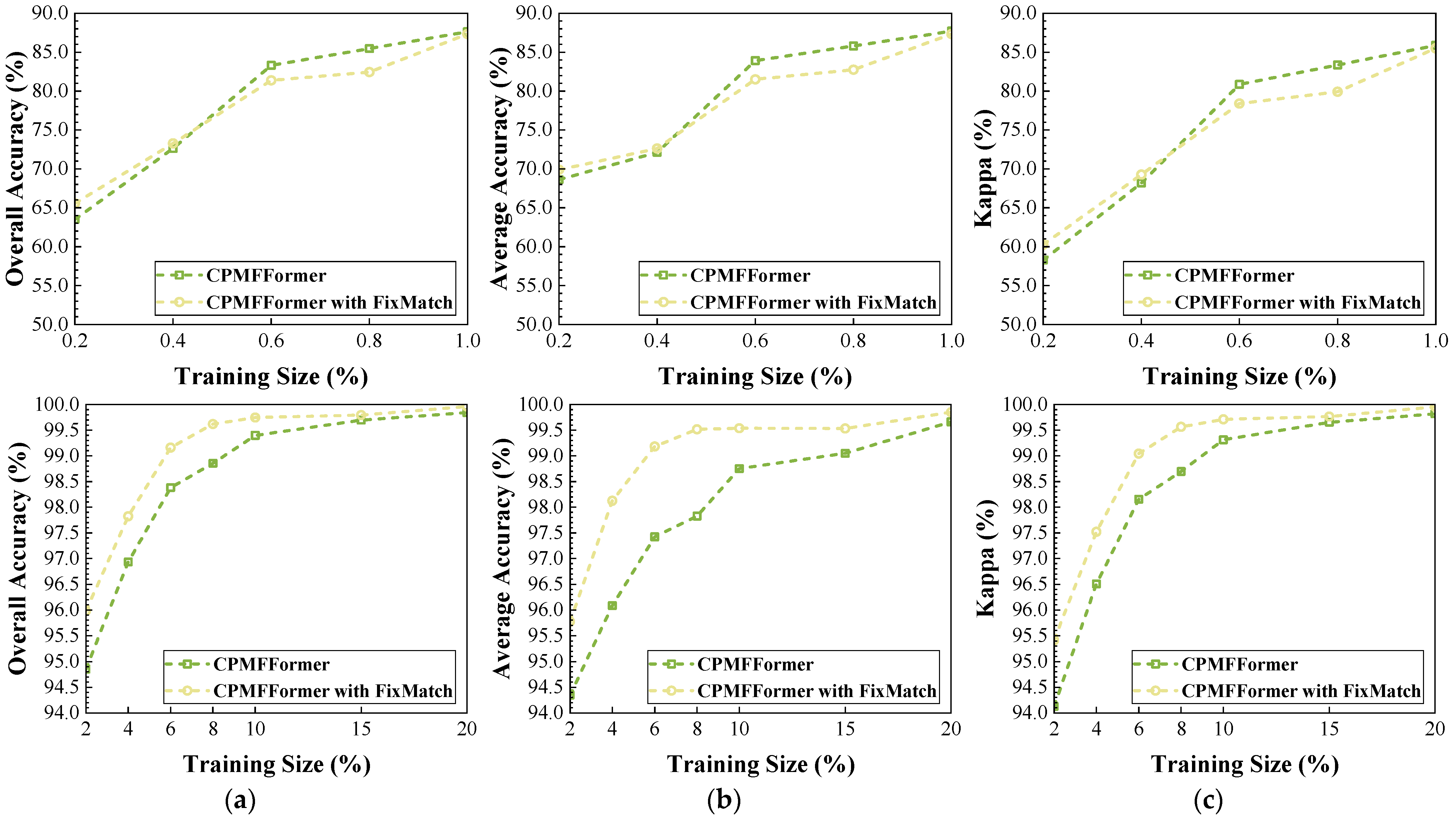
As shown in Figure 19, Figure 20, Figure 21, Figure 22 and Figure 23, the training sample size has a significant impact on classification performance. Taking the Indian dataset as an example, when the training sample size is 0.2%, the OA, AA, and $\kappa$ of CPMFFormer from the Indian dataset are 63.50%,  68.61%, and 58.26%, respectively. When the training sample size is 20%, the OA,  AA, and $\kappa$ of CPMFFormer from the Indian dataset are 99.84%,  99.66%, and 99.82%, respectively. In other words, when there are sufficient training samples, the classification network can usually achieve optimal classification performance. However, in practical applications, the data labeling cost is relatively high. To obtain better classification performance with limited labeled samples, existing research typically introduces semi-supervised learning [52]. Semi-supervised learning is a paradigm that uses both labeled and unlabeled samples for network training. In current research, FixMatch is a representative semi-supervised learning strategy based on pseudo-labels and consistency regularization [53].

To analyze the expandability of CPMFFormer, this section introduces FixMatch into the proposed network and constructs a semi-supervised HSI classification framework that combines labeled and unlabeled samples. The experimental results are shown in Figure 29. In the semi-supervised CPMFFormer, we first use Equation (29) to calculate the supervised loss based on labeled samples. Then, weak and strong augmentations are applied to unlabeled samples to construct the consistency regularization mechanism. Meanwhile, pseudo-labels are generated by predicting the weakly enhanced samples. When the prediction confidence is higher than a preset threshold, the pseudo-label is retained. This section sets the threshold to 0.95. Furthermore, the semi-supervised loss is calculated using the corresponding strongly augmented samples and pseudo-labels according to Equation (29), thereby guiding CPMFFormer to maintain stable predictions on unlabeled data. Finally, the supervised loss and semi-supervised loss are weighted to optimize the network parameters. In this section, the weight is set to 1.

Experimental results show that the classification performance of CPMFFormer is improved across most training sample sizes after introducing FixMatch. This demonstrates that semi-supervised learning can effectively mine spectral–spatial structure information in unlabeled samples. This is beneficial for enhancing the discriminative power and generalization capability of the classification network. When labeled samples are limited, the decision boundary of the supervised network tends to be biased towards the labeled class. The consistency constraint of FixMatch provides additional manifold structure information through unlabeled samples. This guides the classification network to learn a smoother decision boundary in the feature space that better fits the data distribution, thereby improving the stability and robustness of the classification network. Meanwhile, semi-supervised learning can significantly reduce labeling costs. The pixel-level labeling of HSIs typically requires expert involvement and extensive manual review. Semi-supervised learning frameworks can fully use massive unlabeled samples. This makes the classification network more practical in real-world remote sensing scenarios.

Furthermore, we observe that when the training sample sizes are 0.6%, 0.8%, and 1%, the classification performance after introducing FixMatch is slightly lower than that of CPMFFormer. The main reason is likely the use of a fixed high confidence threshold. This may lead to the predictions of CPMFFormer for unlabeled samples being just enough to pass through a large number of pseudo-labels at these three training sample sizes, while the supervised training is insufficient to guarantee the quality of pseudo-labels. This will cause many incorrect pseudo-labels to be used in network training, thereby generating negative transfer and affecting classification performance.

5. Discussion

This section mainly discusses the usage, AI properties and interpretability limitations, adaptive range, and future optimization directions of CPMFFormer, as follows:

Usage: CPMFFormer is suitable for HSI classification tasks that require handling significant spectral variability and complex multiscale spatial structure. It is particularly valuable in the following application scenarios:

(1)

Agricultural fine-grained classification and crop monitoring: By leveraging the capability of CSWM in distinguishing corps with similar spectra but which belong to different classes, CPMFFormer can identify adjacent crop species and field boundaries across large regions of cultivated land. This provides reliable support for crop planting structure surveys, agricultural monitoring, and yield estimation.

(2)

Urban and rural land object recognition: Using CRCM and the progressive multiscale fusion strategy, CPMFFormer can identify multiple types of ground objects in urban and suburban regions with complex spectral–spatial distributions, such as roads, rooftops, green plants, water bodies, etc. It is suitable for urban planning, change detection, and land use monitoring.

(3)

Fine-grained mapping for wetlands and ecological environments: For regions where wetlands, lakes, and farmland intersect, CPMFFormer can maintains stable classification results even under strong interference caused by background noise and mixed pixel conditions. This can support fine-grained mapping for ecological protection and environmental monitoring.

(4)

Other hyperspectral application scenarios: For tasks that require high-precision classification in the presence of significant spectral drift, internal heterogeneity of ground objects, or inhomogeneous spatial texture, CPMFFormer also has strong adaptability and practical value, such as forestry resource surveys, mining region distribution identification, geological surveys, etc.

In summary, CPMFFormer is not designed solely for a single public dataset but rather addresses key challenges such as spectral variability and multiscale spatial structure integration commonly encountered in real remote sensing scenes. Therefore, its usage not only covers typical agricultural, urban, and wetland scenarios validated by public HSI datasets, but can also be extended to other ground object fine-classification tasks that require high-discriminative spectral–spatial features.

AI properties and interpretability: The class-aware spectral weighting enables each ground object to learn a differentiated spectral attention pattern. The spectral weight curves are used to visually demonstrate the decision basis of CPMFFormer. This improves its interpretability. Moreover, the center dependency modeling effectively reflects the contribution of neighboring pixels to the classification decision of the center pixel. This semantic saliency-based filtering mechanism further reduces background and inter-class interference. Combined with the progressive multiscale fusion strategy, CPMFFormer obtains a balance between high performance and low-conflict semantics. It achieves adaptive learning decisions for ground object at the AI algorithm level.

Limitations: Although CPMFFormer maintains a lead in most tasks, its performance degrades when the training sample size is small. According to the classification performance obtained by CPMFFormer with different training sample sizes, when the training sample size is only 0.2%, the OA is reduced by approximately 36% compared with when the training sample size is 20%. In the cross-domain scenarios (e.g., the Houston dataset and the WHU-Hi-HongHu dataset), OA decreases by an average of approximately 4% due to differences in sensor and spectral distribution. Moreover, although CPMFFormer balances classification performance and computational complexity through group convolution and the bottleneck structure, it still incurs significant computational and memory pressure when performing classification in large-scale high-resolution scenarios.

Adaptive range: CPMFFormer is suitable for HSI classification tasks with medium or larger training sample size, significant spectral variability and complex spatial structure. When labeled samples are scarce or cross-sensor and cross-region transfer is required, semi-supervised learning (e.g., pseudo-labeling and consistency regularization), domain adaptation (e.g., distribution alignment or feature transformation), and transfer learning can be combined to enhance generalization performance.

Future optimization directions: Future research will focus on further exploring the combination between CPMFFormer and semi-supervised learning to improve robustness and generalization performance of CPMFFormer. According to the experimental results shown in Figure 29, future research can be mainly carried out in the following aspects:

(1)

Adaptive semi-supervised framework: FixMatch-based semi-supervised learning can effectively use unlabeled samples. However, performance fluctuations at some training sample sizes (e.g., 0.6%, 0.8%, and 1%) indicate the need to introduce adaptive mechanisms. Future research will focus on the dynamic confidence threshold, class-balanced pseudo-label selection, and staged unsupervised weighting strategy. This ensures stable training of the classification network at different supervised levels.

(2)

Spectral consistency augmentation: Current data augmentation may disrupt the band continuity of HSIs. This is particularly crucial for preserving spectral features. Future research will focus on designing spectrally friendly data augmentation strategy and extending consistency regularization to the spectral dimension. This can fully use unlabeled samples while preserving physical meaning.

(3)

CFCL-based pseudo-label selection mechanism: A center-dependent pseudo-label selection method will be constructed based on CFCL. By evaluating the spectral–spatial correlation between unlabeled samples and its center pixel, only samples with high reliability and consistency are selected for training. This can effectively suppress interference from noisy pseudo-labels.

(4)

Pre-training and multi-source data fusion: Advanced semi-supervised or self-supervised pre-training methods will be further introduced. By learning a general spectral–spatial representation on large-scale unlabeled data, the initialization performance for subsequent classification tasks can be optimized.

In summary, future work will focus on building a more adaptive and physically consistent semi-supervised learning framework. This will help achieve higher classification accuracy and stronger generalization ability in real remote sensing scenarios.

6. Conclusions

To reduce the impact of spectral variability and enhance the feature representation capability, this paper proposes CPMFFormer. Since it is difficult for current spectral weighting mechanisms to effectively identify samples with similar spectra, but which belong to different classes, this paper introduces class information to enable learning of class-specific spectral weights. Unlike existing center attention mechanisms, this paper combines CFCL with multiscale convolutional layers. This achieves continuous suppression of interference information at different scales. Furthermore, current multiscale fusion strategies directly fuse features with large-scale differences. This easily leads to information confusion and semantic conflict. This paper designs a progressive multiscale fusion strategy to achieve a smooth semantic transition by gradually fusing adjacent scale features. We compared CPMFFormer with fifteen existing networks. Experiments show that CPMFFormer has better classification performance, stronger network stability, and lower computational complexity. We conducted ablation experiments, which show the effectiveness of the overall network framework and the core design in CPMFFormer.

References

1. Yue, G.; Zhang, L.; Zhou, Y.; Wang, Y.; Xue, Z. S2TNet: Spectral–spatial triplet network for few-shot hyperspectral image classification. IEEE Geosci. Remote Sens. Lett. 2024, 21, 5501705. [Google Scholar] [CrossRef]
2. Lee, E.; Pan, L.; Li, Z.; Bhattacharyya, S.S. Efficient hyperspectral image classification using discrete cosine transform on limited-resource systems. IEEE J. Sel. Top. Appl. Earth Obs. Remote Sens. 2025, 18, 24647–24661. [Google Scholar] [CrossRef]
3. Bourriz, M.; Hajji, H.; Laamrani, A.; Elbouanani, N.; Abdelali, H.A.; Bourzeix, F.; El-Battay, A.; Amazirh, A.; Chehbouni, A. Integration of hyperspectral imaging and AI techniques for crop type mapping: Present status, trends, and challenges. Remote Sens. 2025, 17, 1574. [Google Scholar] [CrossRef]
4. Zhang, T.; Xuan, C.; Ma, Y.; Tang, Z.; Gao, X. An efficient and precise dynamic neighbor graph network for crop mapping using unmanned aerial vehicle hyperspectral imagery. Comput. Electron. Agric. 2025, 230, 109838. [Google Scholar] [CrossRef]
5. García-Vera, Y.E.; Polochè-Arango, A.; Mendivelso-Fajardo, C.A.; Gutiérrez-Bernal, F.J. Hyperspectral image analysis and machine learning techniques for crop disease detection and identification: A review. Sustainability 2024, 16, 6064. [Google Scholar] [CrossRef]
6. Rahmani, N.; Sekandari, M.; Pour, A.B.; Ranjbar, H.; Carranza, E.J.M. Evaluation of support vector machine classifiers for lithological mapping using PRISMA hyperspectral remote sensing data: Sahand–Bazman magmatic arc, central Iran. Remote Sens. Appl. Soc. Environ. 2025, 37, 101449. [Google Scholar] [CrossRef]
7. Wang, Y.; He, L.; He, Z.; Chen, J.; Luo, F. A task-oriented framework for efficient lithological mapping of imbalanced categories using hyperspectral imagery. Int. J. Appl. Earth Obs. Geoinf. 2025, 143, 104749. [Google Scholar] [CrossRef]
8. Tolentino, V.; Ortega Lucero, A.; Koerting, F.; Savinova, E.; Hildebrand, J.C.; Micklethwaite, S. Drone-based VNIR–SWIR hyperspectral imaging for environmental monitoring of a uranium legacy mine site. Drones 2025, 9, 313. [Google Scholar] [CrossRef]
9. Li, Z.; Liu, T.; Lu, Y.; Tian, J.; Zhang, M.; Zhou, C. Enhanced hyperspectral image classification for coastal wetlands using a hybrid CNN-Transformer approach with cross-attention mechanism. Front. Mar. Sci. 2025, 12, 1613565. [Google Scholar] [CrossRef]
10. Ceriani, R.; Brocco, S.; Pepe, M.; Oggioni, S.; Vacchiano, G.; Motta, R.; Berretti, R.; Ascoli, D.; Garbarino, M.; Morresi, D. Hyperspectral and LiDAR space-borne data for assessing mountain forest volume and biomass. Int. J. Appl. Earth Obs. Geoinf. 2025, 141, 104614. [Google Scholar] [CrossRef]
11. Holt, Z.K.; Khan, S.D.; Rodrigues, D.F. Hyperspectral remote sensing as an environmental plastic pollution detection approach to determine occurrence of microplastics in diverse environments. Environ. Pollut. 2025, 377, 126426. [Google Scholar] [CrossRef] [PubMed]
12. Luque-Söllheim, A.; Martín, J.; Medina, A.; Carrasco-Acosta, M.; García-Jiménez, P.; Ferrer, N.; Bergasa, O. Hyperspectral rapid detection of bacterial content and water quality parameters in coastal bathing waters. Mar. Pollut. Bull. 2026, 222, 118705. [Google Scholar] [CrossRef] [PubMed]
13. Arias, F.; Zambrano, M.; Galagarza, E.; Broce, K. Mapping harmful algae blooms: The potential of hyperspectral imaging technologies. Remote Sens. 2025, 17, 608. [Google Scholar] [CrossRef]
14. Ding, S.; Ruan, X.; Yang, J.; Sun, J.; Li, S.; Hu, J. LSSMA: Lightweight spectral–spatial neural architecture with multiattention feature extraction for hyperspectral image classification. IEEE J. Sel. Top. Appl. Earth Obs. Remote Sens. 2024, 17, 6394–6413. [Google Scholar] [CrossRef]
15. Melgani, F.; Bruzzone, L. Classification of hyperspectral remote sensing images with support vector machines. IEEE Trans. Geosci. Remote Sens. 2004, 42, 1778–1790. [Google Scholar] [CrossRef]
16. Ham, J.; Chen, Y.; Crawford, M.M.; Ghosh, J. Investigation of the random forest framework for classification of hyperspectral data. IEEE Trans. Geosci. Remote Sens. 2005, 43, 492–501. [Google Scholar] [CrossRef]
17. Haut, J.; Paoletti, M.; Paz-Gallardo, A.; Plaza, J.; Plaza, A.; Vigo-Aguiar, J. Cloud implementation of logistic regression for hyperspectral image classification. In Proceedings of the 17th International Conference on Computational and Mathematical Methods in Science and Engineering (CMMSE), Cádiz, Spain, 4–8 July 2017. [Google Scholar]
18. Paoletti, M.E.; Haut, J.M.; Plaza, J.; Plaza, A. A new deep convolutional neural network for fast hyperspectral image classification. ISPRS J. Photogramm. Remote Sens. 2018, 145, 120–147. [Google Scholar] [CrossRef]
19. Wei, L.; Ma, H.; Yin, Y.; Geng, C. Kmeans-CM algorithm with spectral angle mapper for hyperspectral image classification. IEEE Access 2023, 11, 26566–26576. [Google Scholar] [CrossRef]
20. Beirami, B.A.; Mokhtarzade, M. Band grouping SuperPCA for feature extraction and extended morphological profile production from hyperspectral images. IEEE Geosci. Remote Sens. Lett. 2020, 17, 1953–1957. [Google Scholar] [CrossRef]
21. Fang, Y.; Ye, Q.; Sun, L.; Zheng, Y.; Wu, Z. Multiattention joint convolution feature representation with lightweight transformer for hyperspectral image classification. IEEE Trans. Geosci. Remote Sens. 2023, 61, 5513814. [Google Scholar] [CrossRef]
22. Wei, Y.-L.; Zheng, Y.-B.; Wang, R.; Li, H.-C. Quaternion convolutional neural network with EMAP representation for multisource remote-sensing data classification. IEEE Geosci. Remote Sens. Lett. 2023, 20, 5508805. [Google Scholar] [CrossRef]
23. Han, Z.; Yang, J.; Gao, L.; Zeng, Z.; Zhang, B.; Chanussot, J. Dual-branch subpixel-guided network for hyperspectral image classification. IEEE Trans. Geosci. Remote Sens. 2024, 62, 5521813. [Google Scholar] [CrossRef]
24. Wei, L.; Liu, Y.; Yin, Y.; Gu, J. Improved transformer network based on multiscale grouping feature fusion for hyperspectral image classification. IEEE J. Sel. Top. Appl. Earth Obs. Remote Sens. 2025, 18, 21305–21325. [Google Scholar] [CrossRef]
25. Shi, C.; Yue, S.; Wang, L. A dual-branch multiscale transformer network for hyperspectral image classification. IEEE Trans. Geosci. Remote Sens. 2024, 62, 5504520. [Google Scholar] [CrossRef]
26. Bai, J.; Shi, W.; Xiao, Z.; Ali, T.A.A.; Ye, F.; Jiao, L. Achieving better category separability for hyperspectral image classification: A spatial–spectral approach. IEEE Trans. Neural Netw. Learn. Syst. 2023, 35, 9621–9635. [Google Scholar] [CrossRef]
27. Duan, Y.; Chen, C.; Fu, M.; Li, Y.; Gong, X.; Luo, F. Dimensionality reduction via multiple neighborhood-aware nonlinear collaborative analysis for hyperspectral image classification. IEEE Trans. Circuits Syst. Video Technol. 2024, 34, 9356–9370. [Google Scholar] [CrossRef]
28. Yang, K.; Sun, H.; Zou, C.; Lu, X. Cross-attention spectral–spatial network for hyperspectral image classification. IEEE Trans. Geosci. Remote Sens. 2021, 60, 5518714. [Google Scholar] [CrossRef]
29. Shu, Z.; Liu, Z.; Zhou, J.; Tang, S.; Yu, Z.; Wu, X.-J. Spatial–spectral split attention residual network for hyperspectral image classification. IEEE J. Sel. Top. Appl. Earth Obs. Remote Sens. 2022, 16, 419–430. [Google Scholar] [CrossRef]
30. Chhapariya, K.; Buddhiraju, K.M.; Kumar, A. A deep spectral–spatial residual attention network for hyperspectral image classification. IEEE J. Sel. Top. Appl. Earth Obs. Remote Sens. 2024, 17, 15393–15406. [Google Scholar] [CrossRef]
31. Han, Z.; Yang, J.; Gao, L.; Zeng, Z.; Zhang, B.; Chanussot, J. Subpixel spectral variability network for hyperspectral image classification. IEEE Trans. Geosci. Remote Sens. 2025, 63, 5504014. [Google Scholar] [CrossRef]
32. Liu, H.; Zhang, H.; Yang, R. Lithological classification by hyperspectral remote sensing images based on double-branch multi-scale dual-attention network. IEEE J. Sel. Top. Appl. Earth Obs. Remote Sens. 2024, 17, 14726–14741. [Google Scholar] [CrossRef]
33. Gao, H.; Sheng, R.; Chen, Z.; Liu, H.; Xu, S.; Zhang, B. Multiscale random-shape convolution and adaptive graph convolution fusion network for hyperspectral image classification. IEEE Trans. Geosci. Remote Sens. 2024, 62, 5508414. [Google Scholar] [CrossRef]
34. Ge, H.; Wang, L.; Liu, M.; Zhao, X.; Zhu, Y.; Pan, H.; Liu, Y. Pyramidal multiscale convolutional network with polarized self-attention for pixel-wise hyperspectral image classification. IEEE Trans. Geosci. Remote Sens. 2023, 61, 5516017. [Google Scholar] [CrossRef]
35. Shi, H.; Zhang, Y.; Cao, G.; Yang, D. MHCFormer: Multiscale hierarchical conv-aided fourierformer for hyperspectral image classification. IEEE Trans. Instrum. Meas. 2024, 73, 5501115. [Google Scholar] [CrossRef]
36. Shu, Z.; Zeng, K.; Zhou, J.; Wang, Y.; Tai, M.; Yu, Z. Spectral-spatial synergy guided attention network for hyperspectral image classification. IEEE Trans. Geosci. Remote Sens. 2025, 63, 5523316. [Google Scholar] [CrossRef]
37. Ma, Y.; Lan, Y.; Xie, Y.; Yu, L.; Chen, C.; Wu, Y.; Dai, X. A spatial–spectral transformer for hyperspectral image classification based on global dependencies of multi-scale features. Remote Sens. 2024, 16, 404. [Google Scholar] [CrossRef]
38. Feng, J.; Wang, Q.; Zhang, G.; Jia, X.; Yin, J. CAT: Center attention transformer with stratified spatial–spectral token for hyperspectral image classification. IEEE Trans. Geosci. Remote Sens. 2024, 62, 5615415. [Google Scholar] [CrossRef]
39. Zhang, M.; Yang, Y.; Zhang, S.; Mi, P.; Han, D. Spectral-spatial center-aware bottleneck transformer for hyperspectral image classification. Remote Sens. 2024, 16, 2152. [Google Scholar] [CrossRef]
40. Chen, N.; Fang, L.; Xia, Y.; Xia, S.; Liu, H.; Yue, J. Spectral query spatial: Revisiting the role of center pixel in transformer for hyperspectral image classification. IEEE Trans. Geosci. Remote Sens. 2024, 62, 5402714. [Google Scholar] [CrossRef]
41. Wang, Y.; Shu, Z.; Yu, Z. Efficient attention transformer network with self-similarity feature enhancement for hyperspectral image classification. IEEE J. Sel. Top. Appl. Earth Obs. Remote Sens. 2025, 18, 11469–11486. [Google Scholar] [CrossRef]
42. Jia, C.; Zhang, X.; Meng, H.; Xia, S.; Jiao, L. CenterFormer: A center spatial-spectral attention transformer network for hyperspectral image classification. IEEE J. Sel. Top. Appl. Earth Obs. Remote Sens. 2025, 18, 5523–5539. [Google Scholar] [CrossRef]
43. Lu, Y.; Zhang, Y.; Jiang, X.; Liu, X.; Cai, Z. Dual-branch convolution-transformer network with spectral-spatial attention for hyperspectral image classification. IEEE Trans. Geosci. Remote Sens. 2025, 63, 5518216. [Google Scholar] [CrossRef]
44. Yu, C.; Zhu, Y.; Wang, Y.; Zhao, E.; Zhang, Q.; Lu, X. Concern with center-pixel labeling: Center-specific perception transformer network for hyperspectral image classification. IEEE Trans. Geosci. Remote Sens. 2025, 63, 5514614. [Google Scholar] [CrossRef]
45. Dosovitskiy, A.; Beyer, L.; Kolesnikov, A.; Weissenborn, D.; Zhai, X.; Unterthiner, T.; Dehghani, M.; Minderer, M.; Heigold, G.; Gelly, S. An image is worth 16x16 words: Transformers for image recognition at scale. arXiv 2020, arXiv:2010.11929. [Google Scholar]
46. Hong, D.; Han, Z.; Yao, J.; Gao, L.; Zhang, B.; Plaza, A.; Chanussot, J. SpectralFormer: Rethinking hyperspectral image classification with transformers. IEEE Trans. Geosci. Remote Sens. 2021, 60, 5518615. [Google Scholar] [CrossRef]
47. Ouyang, E.; Li, B.; Hu, W.; Zhang, G.; Zhao, L.; Wu, J. When multigranularity meets spatial–spectral attention: A hybrid transformer for hyperspectral image classification. IEEE Trans. Geosci. Remote Sens. 2023, 61, 4401118. [Google Scholar] [CrossRef]
48. Zhang, L.; Wang, Y.; Yang, L.; Chen, J.; Liu, Z.; Bian, L.; Yang, C. D2S2BoT: Dual-dimension spectral-spatial bottleneck transformer for hyperspectral image classification. IEEE J. Sel. Top. Appl. Earth Obs. Remote Sens. 2023, 17, 2655–2669. [Google Scholar] [CrossRef]
49. Xu, Y.; Wang, D.; Zhang, L.; Zhang, L. Dual selective fusion transformer network for hyperspectral image classification. Neural Netw. 2025, 187, 107311. [Google Scholar]
50. Chen, Q.; Li, Z.; Yin, J.; Huang, W.; Zhan, T. Local-global feature extraction network with dynamic 3D convolution and residual attention transformer for hyperspectral image classification. IEEE J. Sel. Top. Appl. Earth Obs. Remote Sens. 2025, 18, 9986–10001. [Google Scholar] [CrossRef]
51. Woo, S.; Park, J.; Lee, J.-Y.; Kweon, I.S. CBAM: Convolutional block attention module. In Proceedings of the European Conference on Computer Vision (ECCV), Munich, Germany, 8–14 September 2018. [Google Scholar]
52. Yang, C.; Liu, Z.; Guan, R.; Zhao, H. A Semi-supervised multi-scale convolutional neural network for hyperspectral image classification with limited labeled samples. Remote Sens. 2025, 17, 3273. [Google Scholar] [CrossRef]
53. Sohn, K.; Berthelot, D.; Carlini, N.; Zhang, Z.; Zhang, H.; Raffel, C.A.; Cubuk, E.D.; Kurakin, A.; Li, C.-L. Fixmatch: Simplifying semi-supervised learning with consistency and confidence. In Proceedings of the International Conference on Neural Information Processing Systems, Vancouver, BC, Canada, 6–12 December 2020. [Google Scholar]
Figure 1. Spectral curves of three types of ground objects in the Indian dataset. Each colored curve represents the average spectral response values of all pixels in the corresponding class. The shaded region around each curve represents the standard deviation of spectral response for that class (Corn-Notill: 1428 pixels; Corn-Mintill: 830 pixels; Corn class: 237 pixels).
Remotesensing 17 03684 g001
Figure 2. Activation response heatmaps obtained from the PaviaU dataset using different convolutional kernels: (a) 3 × 3 convolutional kernel; (b) 5 × 5 convolutional kernel; (c) 7 × 7 convolutional kernel; (d) 9 × 9 convolutional kernel. The red box represents the Trees class, and the white box represents the Painted Metal Sheets class.
Remotesensing 17 03684 g002
Figure 3. The self-attention mechanism.
Remotesensing 17 03684 g003
Figure 4. The overall framework of CPMFFormer. CPMFFormer is composed of one CSWM, four CRCMs, and six cross-scale fusion bottleneck transformers (CSFBT). CSWM, CRCM, and CSFBT are used to obtain class-specific spectral weights, features at different scales, and progressive fusion features, respectively. Following CSFBT-6, CPMFFormer uses a global average pooling (GAP) layer, a fully connected (FC) layer, and a S o f t m a x function to predict the final classification result.
Remotesensing 17 03684 g004
Figure 5. The framework of CSWM. CSWM is composed of an aggregation operation, a spectral wight learning block, and a class consistency loss function. The aggregation operation smooths the spectral information differences between intra-class input patches. The spectral weight learning block performs adaptive spectral weighting. The class consistency loss function is used to learn the spectral weight centers of different ground objects and generate class-specific spectral weights.
Remotesensing 17 03684 g005
Figure 6. The framework of CRCM. CRCM is composed of two bottleneck residual blocks. In each bottleneck residual block, two 1 × 1 convolutional layers are used to form the bottleneck structure, and a k t × k t group convolution layer is used to extract features at the tth scale. Moreover, the embedded center feature calibration layer (CFCL) is used to model the dependencies between the center pixel and its neighboring pixels. This helps CRCM to reduce the impact of interference information introduced by abnormal pixels on the classification decision of the center pixel.
Remotesensing 17 03684 g006
Figure 7. The framework of CFCL. CFCL computes the correlations between the center pixel and its neighboring pixels through an inner product attention mechanism. Moreover, CFCL introduces a relative center position encoding to enhance spatial relationship modeling capabilities. This enables CFCL to highlight neighboring pixels that are relevant to the center pixel while suppressing irrelevant background information. This improves the representational capability of the center pixel.
Remotesensing 17 03684 g007
Figure 8. The framework of CSFBT. CSFBT takes adjacent scale features as input. It consists of a channel feature enhancement block (CFEB) and a cross-scale fusion block (CSFB). CFEB models inter-channel dependencies and emphasizes valuable channel features. CSFB uses a multi-head cross-scale dual-dimensional attention (MHCSD2A) mechanism to integrate complementary information across adjacent scale features from both spatial and channel dimensions.
Remotesensing 17 03684 g008
Figure 9. The framework of MHCSD2A. MHCSD2A first maps the input features to different attention heads using five linear projection layers. Then, the cross-scale dual-dimensional attention (CSD2A) mechanism is computed in each head. Finally, the computation results of all heads are concatenated, and a linear projection layer is used to obtain the final output features.
Remotesensing 17 03684 g009
Figure 10. The framework of CSD2A. CSD2A achieves complementary semantic fusion between small-scale features and large-scale features by computing attention from both spatial and channel dimensions. This mechanism introduces the relative position encoding to better model complex spatial relationships and preserves structural details during cross-scale fusion.
Remotesensing 17 03684 g010
Figure 11. Impact of batch size on classification performance: (a) OA; (b) AA; (c) κ .
Remotesensing 17 03684 g011
Figure 12. Impact of learning rate on classification performance: (a) OA; (b) AA; (c) κ .
Remotesensing 17 03684 g012
Figure 13. Impact of patch size on classification performance: (a) OA; (b) AA; (c) κ .
Remotesensing 17 03684 g013
Figure 14. Full-Scene classification results obtained by different networks from the Indian dataset: (a) false-color image; (b) ground truth; (c) S3ARN; (d) PMCN; (e) S3GAN; (f) ViT; (g) SFormer; (h) HFormer; (i) MHCFormer; (j) D2S2BoT; (k) SQSFormer; (l) EATN; (m) CFormer; (n) SSACFormer; (o) CPFormer; (p) DSFormer; (q) LGDRNet; (r) CPMFFormer.
Remotesensing 17 03684 g014aRemotesensing 17 03684 g014b
Figure 15. Full-Scene classification results obtained by different networks using the Houston dataset: (a) false-color image; (b) ground truth; (c) S3ARN; (d) PMCN; (e) S3GAN; (f) ViT; (g) SFormer; (h) HFormer; (i) MHCFormer; (j) D2S2BoT; (k) SQSFormer; (l) EATN; (m) CFormer; (n) SSACFormer; (o) CPFormer; (p) DSFormer; (q) LGDRNet; (r) CPMFFormer.
Remotesensing 17 03684 g015aRemotesensing 17 03684 g015b
Figure 16. Full-Scene classification results obtained by different networks from the HongHu dataset: (a) false-color image; (b) ground truth; (c) S3ARN; (d) PMCN; (e) S3GAN; (f) ViT; (g) SFormer; (h) HFormer; (i) MHCFormer; (j) D2S2BoT; (k) SQSFormer; (l) EATN; (m) CFormer; (n) SSACFormer; (o) CPFormer; (p) DSFormer; (q) LGDRNet; (r) CPMFFormer.
Remotesensing 17 03684 g016aRemotesensing 17 03684 g016b
Figure 17. Full-Scene classification results obtained by different networks from the PaviaU dataset: (a) false-color image; (b) ground truth; (c) S3ARN; (d) PMCN; (e) S3GAN; (f) ViT; (g) SFormer; (h) HFormer; (i) MHCFormer; (j) D2S2BoT; (k) SQSFormer; (l) EATN; (m) CFormer; (n) SSACFormer; (o) CPFormer; (p) DSFormer; (q) LGDRNet; (r) CPMFFormer.
Remotesensing 17 03684 g017aRemotesensing 17 03684 g017b
Figure 18. Full-Scene classification results obtained by different networks from the Salinas dataset: (a) false-color image; (b) ground truth; (c) S3ARN; (d) PMCN; (e) S3GAN; (f) ViT; (g) SFormer; (h) HFormer; (i) MHCFormer; (j) D2S2BoT; (k) SQSFormer; (l) EATN; (m) CFormer; (n) SSACFormer; (o) CPFormer; (p) DSFormer; (q) LGDRNet; (r) CPMFFormer.
Remotesensing 17 03684 g018aRemotesensing 17 03684 g018b
Figure 19. Classification performance obtained by different networks with different training sample sizes from the Indian dataset: (a) OA; (b) AA; (c) κ .
Remotesensing 17 03684 g019
Figure 20. Classification performance obtained by different networks with different training sample sizes from the Houston dataset: (a) OA; (b) AA; (c) κ .
Remotesensing 17 03684 g020
Figure 21. Classification performance obtained by different networks with different training sample sizes from the HongHu dataset: (a) OA; (b) AA; (c) κ .
Remotesensing 17 03684 g021
Figure 22. Classification performance obtained by different networks with different training sample sizes from the PaviaU dataset: (a) OA; (b) AA; (c) κ .
Remotesensing 17 03684 g022
Figure 23. Classification performance obtained by different networks with different training samples sizes from the Salinas datasets: (a) OA; (b) AA; (c) κ .
Remotesensing 17 03684 g023
Figure 24. Impact of different modules on classification performance: (a) OA; (b) AA; (c) κ .
Remotesensing 17 03684 g024
Figure 25. Activation response heatmaps obtained by different CSFBTs from the PaviaU dataset: (a) CSFBT-1; (b) CSFBT-2; (c) CSFBT-3; (d) CSFBT-4; (e) CSFBT-5; (f) CSFBT-6. The red box represents the Trees class, and the white box represents the Painted Metal Sheets class.
Remotesensing 17 03684 g025aRemotesensing 17 03684 g025b
Figure 26. Activation response heatmaps obtained by current multiscale fusion strategies from the PaviaU dataset: (a) concatenation; (b) element-wise addition; (c) attention method in the literature [35]. The red box represents the Trees class, and the white box represents the Painted Metal Sheets class.
Remotesensing 17 03684 g026
Figure 27. Impact of different spectral weighting mechanism on classification performance: (a) OA; (b) AA; (c) κ .
Remotesensing 17 03684 g027
Figure 28. Average spectral weights learned by CSWM and SWL: (ac): average spectral weights learned by SWL for the Corn-Notill, Corn-Mintill, and Corn classes; (df): average spectral weights learned by CSWM for the Corn-Notill, Corn-Mintill, and Corn classes.
Remotesensing 17 03684 g028aRemotesensing 17 03684 g028b
Figure 29. The performance changes in CPMFFormer after introducing FixMatch: (a) OA; (b) AA; (c) κ .
Remotesensing 17 03684 g029