Highlights
What are the main findings?
- A radiation-driven encoding module was developed that effectively preserves physical characteristics and ensures feature robustness under noisy conditions, through spatial attention and covariance pooling.
- An adaptive learnable wavelet transform mechanism was designed to significantly enhance high-frequency edge details, overcoming the blurring issues common in infrared imagery.
What is the implication of the main finding?
- The model enables scene recognition, radiation-aware feature extraction, and edge enhancement, improving matching accuracy and pixel-level precision for downstream tasks such as image fusion.
Abstract
Infrared–visible image matching is a prerequisite for environmental monitoring, military reconnaissance, and multisource geospatial analysis. However, pronounced texture disparities, intensity drift, and complex non-linear radiometric distortions in such cross-modal pairs mean that existing frameworks such as SuperPoint + SuperGlue (SP + SG) and LoFTR cannot reliably establish correspondences. To address this issue, we propose a dual-path architecture, the Environment-Adaptive Wavelet Enhancement and Radiation Priors Aided Matcher (EWAM). EWAM incorporates two synergistic branches: (1) an Environment-Adaptive Radiation Feature Extractor, which first classifies the scene according to radiation-intensity variations and then incorporates a physical radiation model into a learnable gating mechanism for selective feature propagation; (2) a Wavelet-Transform High-Frequency Enhancement Module, which recovers blurred edge structures by boosting wavelet coefficients under directional perceptual losses. The two branches collectively increase the number of tie points (reliable correspondences) and refine their spatial localization. A coarse-to-fine matcher subsequently refines the cross-modal correspondences. We benchmarked EWAM against SIFT, AKAZE, D2-Net, SP + SG, and LoFTR on a newly compiled dataset that fuses GF-7, Landsat-8, and Five-Billion-Pixels imagery. Across desert, mountain, gobi, urban and farmland scenes, EWAM reduced the average RMSE to 1.85 pixels and outperformed the best competing method by 2.7%, 2.6%, 2.0%, 2.3% and 1.8% in accuracy, respectively. These findings demonstrate that EWAM yields a robust and scalable framework for large-scale multi-sensor remote-sensing data fusion.
1. Introduction
In recent years, the rapid advancement of Earth observation satellites has generated massive amounts of remote sensing imagery data with varying resolutions. Integrated processing techniques for multi-source remote sensing imagery have gained widespread application [1]. Currently, heterogeneous remote sensing technology has been widely applied in key fields such as land resource monitoring [2], environmental assessment [3], and landslide monitoring [4]. Capitalizing on their superior spatial resolution and rich spectral information, visible-band images are highly effective for detailed terrain identification and vegetation coverage mapping [5,6]. Infrared imagery, conversely, leverages radiometric properties for vegetation monitoring [7], surface temperature inversion [8], and water body identification [9]. The fundamentally different imaging principles underlying these two sensor types produce markedly distinct texture representations at corresponding geographical locations. In visible light images, features manifest as distinct contours, shapes, and structures, thereby easing the recognition of object boundaries. Conversely, infrared imagery is characterized principally by its representation of radiation distribution patterns. The grayscale distribution reveals highly complex and nonlinear relationships. Regarding texture structure, the lower spatial resolution of infrared images results in blurred edges, making it difficult to match the fine features found in visible light images. This renders the identification of homogeneous points extremely challenging [10]. The integration of these two image types has been demonstrated to enhance the precision and completeness of remote sensing information analysis [11,12], providing a robust foundation for multimodal applications.
It is widely accepted that multimodal image registration algorithms are often adapted from conventional image matching methods [13]. Feature-based approaches consist of four steps: feature point detection, feature description, matching and homography estimation [14]. Representative algorithms for the traditional approach include SIFT [15], which builds on the scale invariant feature transform. This algorithm firstly extracts matching points in image, then localizes them using Gaussian difference function selecting the key position, also calculates the direction of matching points with image gradient information and finally constructs a scale and rotation invariant descriptor to accomplish image matching. The ORB method was proposed by Ethan Rublee et al. [16]. It uses a binary descriptor for improved keypoint matching and orientation, offering excellent real-time performance, robustness, and low computational cost. Pablo Fernandez Alcantarilla et al. [17] proposed the AKAZE algorithm, which aims at extracting stable matching points that are invariant to rotations by building a non-linear scale space using an explicitly defined diffusion equation.
Additionally, a series of improved algorithms have been developed based on traditional methods. For example, Dai et al. proposed a progressive SIFT matching algorithm [18]. The algorithm first utilizes the relative scale and principal direction between matching points as constraints to extract initial matching pairs. Subsequently, a Delaunay triangulation is constructed to establish a local geometric constraint model through point diffusion. Finally, by combining the principal direction of matching points, the minimum Euclidean distance criterion, and the local RANSAC algorithm for mismatch elimination, the method achieves high-precision and large-scale matching on heterogeneous optical satellite imagery exhibiting significant scale and rotation differences. To achieve effective registration between optical and SAR images, Xiang and Wang improved the traditional SIFT algorithm [19]. This improved algorithm employs nonlinear diffusion filtering to construct the image scale space, thereby better suppressing speckle noise in SAR imagery while preserving edge information. Simultaneously, it utilizes multi-scale Sobel operators and multi-scale Ratio of Exponentially Weighted Average (ROEWA) operators to compute more uniform gradient information. Based on this consistent gradient information, Harris matching points are extracted, thereby enhancing the stability and uniformity of the matching points. The descriptor construction was also normalized to overcome nonlinear radiometric variations between images, ultimately yielding accurate matching pairs through bilateral FLANN search and RANSAC. Xi et al. proposed the SIFT-ORB Fusion Operator [20] to address the inconsistency in feature extraction between infrared and visible images from UAVs caused by spectral differences. The approach retains the rotation-invariant descriptor advantage of SIFT while leveraging ORB’s high-speed matching capability based on the Hamming distance, thereby achieving complementarity: High-texture regions employ SIFT to ensure accuracy, while low-texture regions switch to ORB to enhance efficiency. Numerous other improvements to traditional image matching algorithms [21,22,23] have also been designed to handle various complex imaging scenes. However, most such methods rely on manually designed feature descriptors, which still struggle to effectively represent the complex features present in heterogeneous images [24].
With the rapid advancement of deep learning, numerous effective methods have been proposed for image matching [25,26,27]. Among them, SuperPoint [28] is a deep learning-based framework for feature detection and descriptor extraction. It employs convolutional neural networks (CNNs) to produce the keypoints and their descriptors so that computation of high quality feature representation becomes efficient. This method demonstrates stable feature representations and strong cross-view matching performance. SuperGlue [29] is an advanced extension of SuperPoint. It employs graph neural networks (GNNs) to model feature matching by formulating the task as a graph matching problem. By implicitly learning spatial relationships and perceptual similarities between feature pairs, SuperGlue achieves superior performance in complex image matching scenarios, significantly enhancing both the accuracy and robustness of the matching results.
As a deep learning-based image matching method, the LoFTR [30] follows a two-stage framework including coarse matching and fine matching. This method effectively addresses matching difficulties of traditional methods in complex scenes under large baselines, lighting changes as well as viewpoint variations by combining local features with Transformer [31] architecture. However, it was not designed for multisensor remote sensing images that contain infrared and visible light. Due to large grayscale differences and significant radiometric fluctuations, the model often generates spurious matches or fails to locate reliable correspondences. Consequently, in this paper, we propose the EWAM model to address the inconsistency between infrared and visible remote sensing images.
2. Methods
2.1. EWAM Model Principle
2.1.1. Dual-Channel Radiation Feature Alignment Network
We propose the EWAM model while retaining LoFTR’s coarse-to-fine matching backbone. EWAM introduces a dedicated feature extraction branch that separately handles visible and infrared data (overall pipeline shown in Figure 1). The rationale is that using a shared feature extraction pipeline for both modalities fails to account for their inherent disparities. This prevents the network from capturing infrared-specific cues, such as unique radiation signatures and distinct grayscale statistics. This problem is exacerbated by significant texture mismatch [32]. To mitigate cross-modal gap, we isolate parameters by embedding the Environment-Adaptive Radiation Feature Extractor and the Wavelet Transform High-Frequency Enhancement Module into the infrared pathway. Each residual block is tagged with its modality, allowing convolutions to learn modality-specific kernels, sharpen edges, and boost target saliency. Infrared images are processed by the Wavelet Transform High-Frequency Enhancement Module and, in parallel, fed into the Environment-Adaptive Radiation Feature Extractor for selective radiation encoding. The infrared branch thus yields an aggregated radiation representation. Finally, both modalities are fused within the pipeline for joint feature extraction, followed by coarse-to-fine matching.
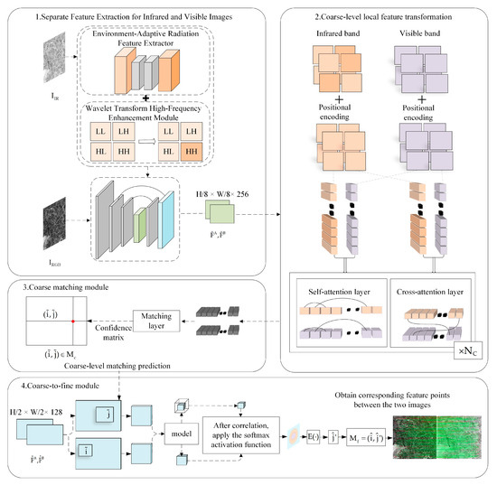
Figure 1.
EWAM Network Architecture.
As illustrated in Figure 1, features are separately extracted from visible images and infrared images . The is concurrently processed through the Environment-Adaptive Radiation Feature Extractor and the Wavelet Transform-Based High-Frequency Enhancement Module. This feature fusion process is applied exclusively to generate coarse-level feature maps. The coarse-level feature map for the infrared image is derived from the fused representation produced by these modules, whereas the coarse-level feature map for the visible image is extracted directly from without this fusion process. Both feature maps have a spatial resolution of H/8 × W/8 of the original image. and denote the fine-level feature maps derived from and at a spatial resolution of, at H/2 × W/2 relative to the original image. denotes the number of LoFTR local feature transformation modules. denotes the locations of matches where the confidence matrix exceeds the given threshold; denotes the expectation function of a probability distribution. denotes the predicted matching entries of the fine-level matching prediction matrix.
2.1.2. Design of the Environment-Adaptive Radiation Feature Extractor
Due to the significant radiation inhomogeneity of terrestrial features across the infrared spectrum in different scenes [33], the infrared radiation intensity in a typical farmland scene is primarily governed by solar heating. This results in a relatively uniform daytime temperature distribution, where global thermal statistics, such as the mean and variance, provide limited discriminative power [34]. However, in environments such as the gobi, Desert, rocks and water bodies exhibit pronounced differences in radiation intensity even at the same temperature. This discrepancy undermines the stability of the correlation between infrared features and visible textures [35]. To this end, we design an Environment-Adaptive Radiation Feature Extractor as shown in Figure 2. The module incorporates a hierarchical radiation prior extractor together with a dynamic feature injection mechanism, enabling the extraction of global radiation statistics from raw infrared imagery. It encodes physical properties of the target such as mean radiation intensity and entropy of the distribution, thus compressing the radiation distribution into a compact physical prior vector. To improve computational efficiency, an adaptive dynamic control strategy is incorporated into the module: if the variance of the infrared image falls below a given threshold such as in a farmland scene, the radiation feature fusion process is skipped. The injection of radiation prior features is activated only in scenes with significant radiation heterogeneity, such as the gobi, desert, where the radiation prior acts as a self-supervised signal. This approach prevents the injection of invalid features by constraining the physical plausibility of infrared features, while simultaneously enhancing their physical interpretability.
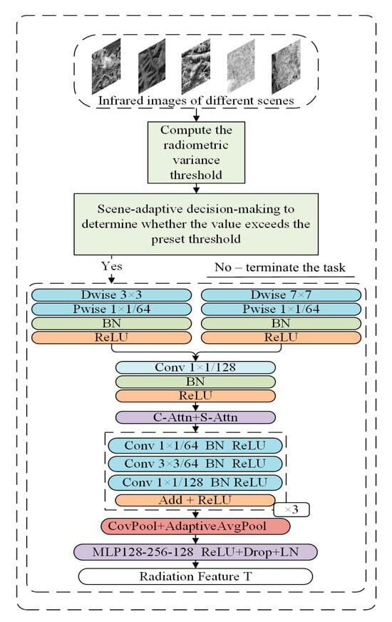
Figure 2.
Environment-Adaptive Radiation Feature Extractor.
When the variance of the infrared image is small, it indicates a uniform radiation field distribution, and differences between radiation features are minimal, making them difficult to distinguish. Therefore, the step of extracting radiation characteristics is skipped. High variance implies significant differences in radiation intensity across the image, corresponding to well-defined edges and structures. During feature extraction, the model uses 7 × 7 and 3 × 3 depthwise-separable convolutional kernels for multi-scale convolution, to capture edge, texture, and long-range radiation features. Adopting a larger receptive field facilitates the integration of neighborhood information, enabling robust estimation of overall radiation distribution in the initial processing stage. Then the two feature maps are combined by a 1 × 1 convolution to produce an output of 128 channels. After normalization and ReLU activation, a channel-wise and spatial attention mechanism refines radiation-related information while suppressing background noise. Nonlinear representation enhancement is performed using a residual bottleneck. Adaptive average pooling and covariance pooling are then applied to generate features, where the latter employs a covariance matrix to preserve the correlation structure of radiation distribution while enhancing the representation of radiation characteristics for objects such as the Gobi, deserts, and rock formations. Finally, the MLP bottleneck (including ReLU, Dropout, and LayerNorm) performs nonlinear transformation and regularization, outputting the global radiation feature vector T, which is fed into downstream stages to highlight structural dissimilarities. In other scenes, radiation characteristics are not introduced, thereby effectively mapping infrared physical properties to a common representation space aligned with visible light features. This mitigates modal differences and ultimately achieves compact physical perception feature encoding through multi-stage transformations.
Infrared Feature Formulation:
In Equation (1), denotes the local radiation saliency feature, denotes the spatially adaptive weight.
The local variance is estimated on the input infrared image within a sliding window:
In Equation (2), denotes the mean within the window. K denotes the number of pixels within the window. denotes the radiation intensity of pixels in the infrared image. denotes the average value of the total thermal radiation across the entire image. The calculation formula is:
2.1.3. Design of the Wavelet Transform High-Frequency Enhancement Module
During acquisition, infrared images, often degraded by radiometric distortions and noise, typically exhibit blurry edges, loss of texture information, and reduced spatial resolution. Consequently, accurately determining homologous points in corresponding visible-light imagery after feature extraction is challenging. To address this issue, we designed the Wavelet Transform High-Frequency Enhancement Module, as shown in Figure 3. This module combines the wavelet transform [36] with a learnable filter.

Figure 3.
Wavelet Transform High-Frequency Enhancement Module.
This module employs the discrete wavelet transform (DWT) to decompose the image into one low-frequency and three high-frequency sub-bands. Candidate bases for this decomposition include the Haar, Daubechies (Db), Coiflet (Coif), and Symlet (Sym) wavelets, as well as the dual-tree complex wavelet transform (DT-CWT) [37]. The selection of these bases is governed by properties such as support length, number of vanishing moments, smoothness, and frequency localization. Haar wavelets exhibit low computational complexity but poor smoothness, potentially reducing the accuracy of high-frequency edge extraction. Coiflet and higher-order Daubechies wavelets possess more vanishing moments, yielding smoother basis functions that enhance edge representation at the cost of increased computational complexity. The DT-CWT is approximately shift-invariant and directionally selective, yet it is computationally intensive.
The Daubechies-4 (Db4) wavelet is selected for its optimal trade-off among spatial localization, smoothness, and computational efficiency. The Db4 wavelet possesses a sufficient number of vanishing moments to capture fine-scale edge and texture information while maintaining low computational complexity, making it suitable for large-scale thermal datasets. This selection facilitates robust extraction of terrain structures such as ridgelines, riverbanks, cliffs, building facades, and corner lineaments in complex natural scenes. According to the principle of edge localization, the image signal is decomposed into high- and low-frequency components. Adaptive learning dynamically optimizes high-frequency enhancement in a computationally efficient manner. This approach overcomes the limitations of manually defined parameters, which often degrade efficiency and impair generalization.
The decomposition and reconstruction process is described as follows:
In Equation (4), LL denotes the low-frequency subband, which reflects the average radiative properties of the target region and captures slow spatial variations in radiation caused by surface materials, solar irradiation, or environmental conditions. For example, in farmland scenes, LL exhibits a relatively uniform radiation field, primarily due to extensive vegetation coverage, whereas in desert or rocky terrains, it highlights large-scale differences in radiation intensity among features such as sand dunes, rocks, and sparse vegetation. LH denotes the horizontal gradient (vertical edge). In terrain feature analysis, it is commonly used to identify boundaries with distinct horizontal extension characteristics, such as ridgelines and riverbanks [38]. HL denotes the vertical gradient (horizontal edge). In practical scenes, this component highlights vertical features such as building facades, steep cliffs, and tree outlines [39]. HH denotes the diagonal gradient (corners and diagonal edges). This information can reveal the arrangement or structure of landforms along diagonal directions, such as sloping terrain surfaces and extended slope vegetation [40].
In Equation (5), denotes the parameterized high-frequency enhancement function.
The input high-frequency subband is processed to extract local edge features via a 3 × 3 convolution kernel. The corresponding formula is:
In Equation (7), denotes the convolution sum and weights, with each kernel extracting edges in a specific direction. is the pixel value of the input subband at position , k denotes the output channel index of the convolution kernel, and is used to adaptively learn the local edge statistical characteristics in infrared images.
Noise Filtering Formula:
In Equation (8), A denotes the activated feature map, which preserves edges with positive gradients while filtering out noise with negative gradients, such as false edges caused by radiation diffusion. Principle: Radiation noise is more pronounced in regions with negative gradients. By applying zero-thresholding to suppress noise while preserving positive gradient structures such as ridgelines, low-gradient noise is filtered out.
Feature Fusion and Edge Reconstruction Formula:
In Equation (9), denotes the fusion weight that strengthens the diagonal edges and corner points, denotes the output bias, achieving adaptive sharpening by dynamically learning the contribution weights of different edges, Low-Frequency Noise Suppression: Performs noise suppression by learning the balance between edge sharpening and low-gradient noise filtering through gradient backpropagation.
Add an adaptive threshold formula to the low-frequency subband LL:
In Equation (10), denotes the noise variance (estimated via local variance estimation), suppressing low-frequency interference caused by texture diffusion, N is the number of pixels in the window.
Noise variance formula:
In Equation (11), denotes the learnable noise sensitivity coefficient (optimized via backpropagation); V is a local sliding window variance estimation. Purpose: Suppress radiation diffusion and filter out background noise in the low-frequency subband. Edge-strengthened backpropagation formula:
In Equations (12) and (13), denotes the learning rate, L denotes the loss function, which combines mean squared error, noise suppression loss, and diagonal edge enhancement loss, with different weighting ratios.
Loss function formula:
In Equation (14), denotes the mean squared error, denotes the noise suppression loss. The weighting coefficients are set as α = 1.0, β = 0.5, γ = 0.2. These values were determined empirically to balance reconstruction accuracy, noise suppression, and directional edge enhancement across different thermal scenes.
Formula:
Purpose: To constrain overall quality and ensure structural consistency between the wavelet transformed image and the original image.
Formula:
denotes the directional perception loss. To further strengthen the structural consistency of high-frequency reconstruction, a directional perceptual loss is defined on the diagonal high-frequency subband HH. This loss constrains the reconstructed diagonal structures to align with their original orientation-dependent responses. Specifically, the HH subband is filtered using 3 × 3 directional kernels to extract responses along two dominant diagonal directions, 45° and 135°. The two enforced directions correspond to the principal diagonal orientations represented in the HH subband of the single-tree DWT. Since the standard DWT combines both diagonal components within HH, the supervision at 45° and 135° provides an effective approximation for enhancing diagonal and corner structures without introducing additional computational cost. denoted as formula:
In Equation (17), denotes the high-frequency subband in a specific direction. Purpose: targeted edge enhancement with directional adaptability. Advantages: Data-driven learning of infrared edge characteristics outperforms fixed operators.
3. Results
3.1. Experiments and Results Analysis
3.1.1. Experimental Environment and Dataset
To validate the proposed method’s performance, we conducted experiments on matching infrared and visible remote sensing images across various scenes. The experimental environment is detailed in Table 1. The experiments utilized publicly available datasets, including the Five-Billion-Pixels dataset [41] (captured by the Gaofen-2 PMS camera, covering over 5000 km2 across more than 60 cities in China and encompassing scenes such as paddy fields, urban residential areas, and bare land), the Thermal Infrared and Multispectral Image Dataset [42] (hereinafter referred to as TIAMID, containing 3668 thermal infrared and multispectral images from diverse scenes), Gaofen-7 (GF-7) satellite imagery, and 2750 raw images from the Landsat 8 satellite. Together, these datasets form the foundational dataset for this study. All image pairs were acquired simultaneously over the same geographic locations and were cropped or resampled to a standardized resolution of 840 × 840 pixels to ensure spatial consistency. The model was trained using the AdamW optimizer with an initial learning rate of 6 × 10⁻⁴. The batch size was set to 8, and training proceeded for 200 epochs, with the learning rate decaying by a factor of 0.1 every 50 epochs. All experiments were conducted using fixed random seeds to ensure reproducibility.

Table 1.
Experimental Environment.
Examples from the datasets are illustrated in Figure 4, with visible light images on the left and corresponding infrared images on the right. The comparison models include SIFT, AKAZE, D2-Net, SP + SG, LoFTR, and our proposed model, making a total of six models.
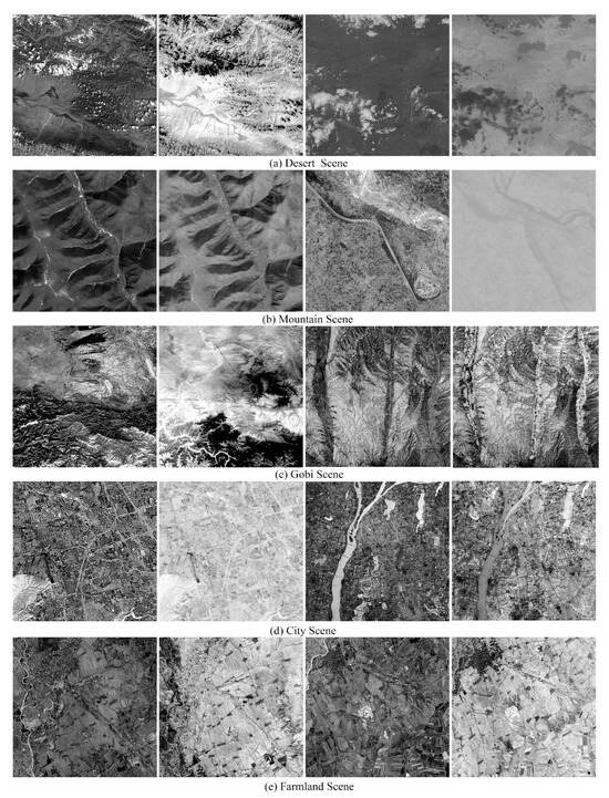
Figure 4.
Data Presentation of Each Scene.
3.1.2. Baseline and Indicators
The evaluation metrics are described as follows:
For low-quality IR scenes such as desert, mountain, and gobi, where noise is significant, the maximum number of detected matching points was set to 1000. In city and farmland scenes, the textures are relatively simple, radiation variations are minimal, and global features are well defined; therefore, the maximum number of matching points was fixed at 1500.
Precision: It is defined as the ratio of correctly matched points to the total number of matching points:
In Equation (18): TMP denotes the total number of matching points; NCM denotes the total number of correct matching points obtained through the statistical matching algorithm.
The correctness of each matching point is determined by calculating the deviation between the matched coordinates and the theoretical coordinates, as defined by the following formula:
In Equation (19): denotes the point pairs obtained by the matching algorithm; denotes theoretical coordinates; ε denotes the error threshold. The experimental error is set to 3 pixels. Connection lines corresponding to matching points with errors less than or equal to the threshold are displayed in green, whereas those exceeding the threshold are shown in red.
RMSE: Root Mean Square Error of Matching Points, a commonly used metric for evaluating matching algorithm performance, measures the degree of discrepancy between predicted and actual values for matching points. The calculation formula is expressed as follows:
In Equation (20): denotes the ground-truth location. denotes the predicted correspondence.
3.2. Infrared and Visible Light Band Image Matching Across Different Scenes
The scene tests were based on the Five-Billion-Pixels classification dataset and were divided into five scenes: desert, mountain, gobi, city and farmland. Visible images were synthesized using the red, green, and blue multispectral bands of the Gaofen-7 (GF-7) satellite, together with its near-infrared band. Additionally, composite visible images (Bands 4, 3, and 2 for red, green, and blue, respectively) and Band 11 as the infrared band from Landsat 8 imagery, together with the TIAMID dataset, were used for testing.
3.2.1. Matching Results Visualization
Desert scene (Figure 5): In this scene, the high intensity of visible light and the low intensity of infrared radiation cause grayscale inversion, leading to distorted gradient direction histograms and blurred infrared boundary textures. SIFT and AKAZE failed to identify a sufficient number of reliable matching points. The D2-Net exhibited poor performance in shaded areas, resulting in a large number of erroneous matching points in the lower portion of the image. The proposed model achieved the highest accuracy compared with other methods and produced no significant erroneous matches.
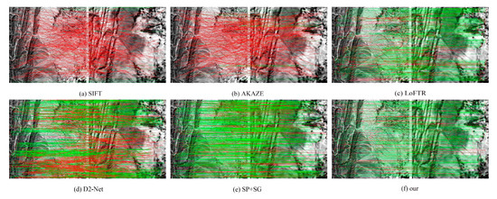
Figure 5.
Comparison of Desert Scene Matching Results. Green: correct matches, error ≤ 3 pixels; Red: incorrect matches, error > 3 pixels.
Mountain Scene (Figure 6): Extensive vegetation reduces light reflectivity, causing the brightness of the visible band to decrease relative to that of the infrared band. This phenomenon consequently affects the accuracy of matching algorithms based on grayscale values. SIFT and AKAZE identified only a small number of valid matching points. However, in mountain terrain, significant geometric distortions caused by parallax and shadow differences between the infrared and visible bands result in systematic shifts at ridges and valleys. Compared with LoFTR, the proposed model shows no obvious matching errors in the upper half of the image, and its matching points are distributed more uniformly across the image.
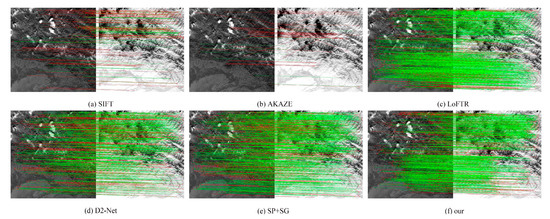
Figure 6.
Comparison of Mountain Scene Matching Results. Green: correct matches, error ≤ 3 pixels; red: incorrect matches, error > 3 pixels.
Gobi Scene (Figure 7 and Figure 8): The terrain boundaries in the Gobi 1 scene are indistinct and irregularly distributed. The Gobi 2 scene exhibits continuous and similar terrain texture characteristics; thus, the Gobi scenes are classified into two types. SIFT and AKAZE failed to detect reliable matching points. The number of matching points identified by the D2-Net method in the Gobi 2 scene decreased significantly, with the points concentrated in the central region of the image. LoFTR produced a large number of errors in the imagery above the Gobi 2 scene. The proposed model achieves high accuracy and uniform feature point extraction in both Gobi scenes.
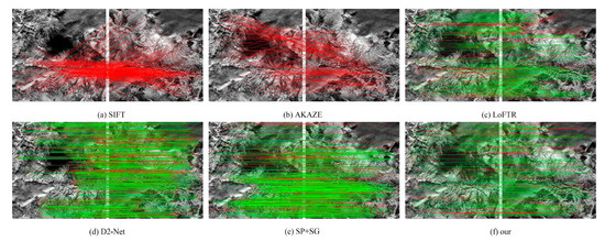
Figure 7.
Comparison of Gobi 1 Scene Matching Results. Green: correct matches, error ≤ 3 pixels; red: incorrect matches, error > 3 pixels.
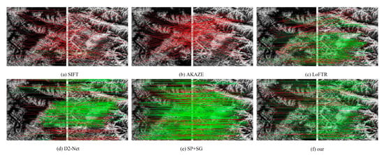
Figure 8.
Comparison of Gobi 2 Scene Matching Results. Green: correct matches, error ≤ 3 pixels; red: incorrect matches, error > 3 pixels.
City Scene (Figure 9): In the City Scene, where structures such as buildings are predominantly regular objects, they possess a greater number of texture features and characteristic points. All six methods exhibited enhanced matching performance compared with those in other scenes. The proposed model matches more points than other methods while maintaining a more dispersed overall line pattern, enabling it to detect feature points in scenes more uniformly.
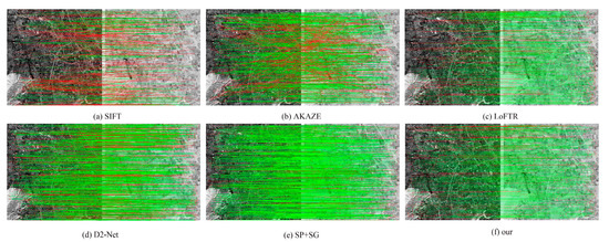
Figure 9.
Comparison of City Scene Matching Results. Green: correct matches, error ≤ 3 pixels; red: incorrect matches, error > 3 pixels.
Farmland Scene (Figure 10): This scene, typically featuring regularly repeating roads, fields and similar elements, shares similarities with the City Scene and is characterized by textural features and a high density of matching points. In this scene, SIFT and AKAZE could only find a limited number of matching points. The proposed model uniformly extracted a large number of matching points across the image. Our method identified a considerable number of highly accurate matching points across all five scenes and demonstrated strong robustness, particularly in sparse-texture environments.
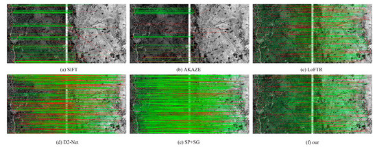
Figure 10.
Comparison of Farmland Scene Matching Results. Green: correct matches, error ≤ 3 pixels; red: incorrect matches, error > 3 pixels.
3.2.2. Quantitative Performance Metrics
Table 2, Table 3, Table 4, Table 5, Table 6 and Table 7 presents the matching results for five scenes, including the total number of detected matching points, matching accuracy, RMSE of matching points, and matching time. These metrics serve to evaluate algorithm performance. All results are reported as mean ± standard deviation over three independent runs. “N/A” denotes RMSE values excluded due to exceeding the statistical threshold.

Table 2.
Desert Scene Matching Results.

Table 3.
Mountain Scene Matching Results.

Table 4.
Gobi 1 Scene Matching Results.

Table 5.
Gobi 2 Scene Matching Results.

Table 6.
City Scene Matching Results.

Table 7.
Farmland Scene Matching Results.
Desert scene (Table 2): D2-Net exhibited an increase in RMSE due to excessive mismatched points. The SP + SG identified only 891 matching points, failing to reach the preset upper limit for matching points. The proposed model achieved a 2.7% improvement in precision compared to LoFTR. LoFTR failed to correctly identify the corresponding matching points between the two images, resulting in an excessively high RMSE. In contrast, the proposed method achieved a uniform point distribution with no obvious erroneous matching pairs.
Mountain scene (Table 3): SIFT, AKAZE, D2-Net, and SP + SG failed to locate the preset number of matching points and demonstrated lower accuracy than LoFTR and the proposed method. The accuracy of the proposed model was 2.6% higher than that of the LoFTR method.
Gobi Scenes (Table 4 and Table 5): D2-Net failed to reach the preset number of matching points in the Gobi 2 scenes. SP + SG achieved high accuracy in two gobi scenes but fell below LoFTR. The accuracy of the proposed model was 1.8% and 2.3% higher than that of the LoFTR, respectively, while its RMSE was significantly lower. This is because, in the two Gobi scenes, the significant difference in visible and infrared texture grayscale in the upper half of the scene, combined with radiation distortion issues, prevented any targeted feature extraction analysis. The LoFTR generated a large number of false matches, leading to a significant increase in RMSE and a decline in matching point accuracy.
City scene (Table 6): In this scene, SIFT, AKAZE, D2-Net, and SP + SG all failed to achieve the target of 1500 matching points. The proposed method and LoFTR were able to identify a greater number of matching points with higher uniformity and accuracy. In this scene, the proposed method achieved 1.4% higher matching point accuracy than LoFTR.
Farmland scene (Table 7): SIFT and AKAZE detected only a small number of matching points, and similar to D2-Net, they failed to reach the preset number of matches. In this scene, SP + SG achieved higher accuracy than LoFTR but remained 1.8% lower than the proposed method. The distribution of matching points identified by the proposed method in this scene was uniform, showing no significant clustering.
As shown in Table 2, Table 3, Table 4, Table 5, Table 6 and Table 7, our method outperformed the highest-accuracy methods in other categories by 2.7%, 2.6%, 2.0%, 2.3%, and 1.8%, respectively, across desert, mountain, gobi, city, and farmland scenes. This method can detect a large number of high-quality valid matching points across these five scenes. While its runtime was slightly longer than LoFTR, the extracted matching points exhibit a more uniform distribution compared to other models, with no obvious errors and the best matching performance.
3.3. Ablation Experiment
To validate the effectiveness of each module, we conducted ablation experiments in three typical challenging environments: desert, mountain, and gobi scenes. The maximum number of matching points was uniformly set to 1000 to ensure comparability of results.
The following four methods were compared:
- Use the original LoFTR model as the baseline.
- LoFTR with Two-Image Separation Feature Extraction, Infrared Band + Wavelet Transform High-Frequency Enhancement Module. This module employs learnable convolutional kernel weights to enhance textures in high-frequency regions through wavelet transformation.
- LoFTR with Two-Image Separation Feature Extraction, Infrared Band + Environment-Adaptive Radiation Feature Extractor. This module determines the current scene based on image radiation intensity, enabling dynamic extraction of radiation features.
- LoFTR with Two-Image Separation Feature Extraction, Infrared Band + Wavelet Transform High-Frequency Enhancement Module + Environment-Adaptive Radiation Feature Extractor.
3.3.1. Qualitative Results Analysis
The associated qualitative comparison results for the three scenes are depicted in Figure 11, Figure 12 and Figure 13. The comparison of results indicates that Solution 2 achieves higher matching point accuracy across all three scenarios, with no significant connection errors observed. Solution 3 outperformed Solution 2 in all three scenes in terms of matching point rate, particularly excelling in the desert and mountain scenes. However, due to the blurred boundaries and considerable texture differences in infrared images, some errors occurred during the matching process. In the mountain scene, mismatches were most evident in the central region, where many match lines deviated with larger inclinations compared to correct matches.
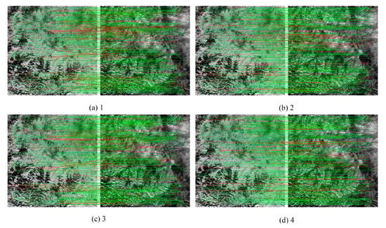
Figure 11.
Desert Scene Matching Results Comparison. Green: correct matches, error ≤ 3 pixels; red: incorrect matches, error > 3 pixels.
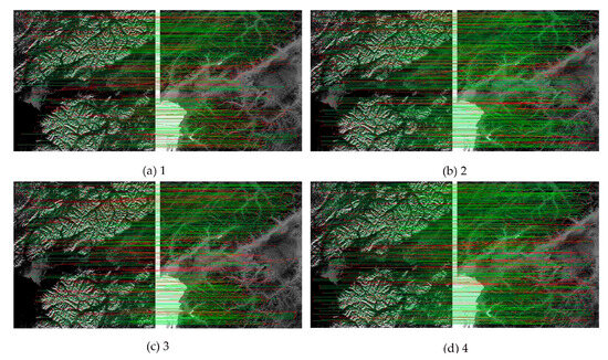
Figure 12.
Mountain Scene Matching Results Comparison. Green: correct matches, error ≤ 3 pixels; red: incorrect matches, error > 3 pixels.
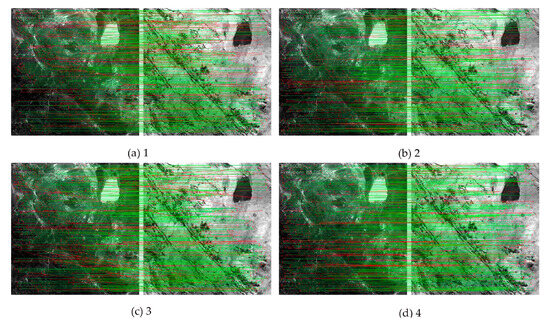
Figure 13.
Comparison of Gobi Scene Matching Results. Green: correct matches, error ≤ 3 pixels; red: incorrect matches, error > 3 pixels.
3.3.2. Quantitative Results Analysis
Using NCM, precision, and RMSE as evaluation metrics yielded detailed matching results for three scenes in Table 8, Table 9 and Table 10.

Table 8.
Comparison Of Desert Scene Matching Results.

Table 9.
Comparison of Mountain Scene Matching Results.

Table 10.
Comparison of Gobi Scene Matching Results.
The Wavelet Transform High-Frequency Enhancement Module primarily improved matching accuracy. In all scenes, Solution 2 achieved lower RMSE values than the baseline, with values of 1.61, 1.79, and 1.81, respectively. This improvement enhanced texture representation, thereby increasing the positional accuracy of the matching points.
The core function of the Environment-Adaptive Radiation Feature Extractor is to enrich the feature representation with discriminative radiation statistics, which contributes to the overall improvement in matching precision. Solution 3 achieved precision improvements of 2.0%, 2.6%, and 4.3% over the baseline across the three scenes, demonstrating that the module effectively extracts and preserves more matching points. However, when used alone, the RMSE in the desert and mountain scenes was slightly higher than that of the baseline model. This occurred because blurred or distorted edge features were retained, and blurring in infrared textures amplified errors, failing to resolve positioning inaccuracies.
Solution 4 combines the strengths of both modules and achieves the highest accuracy across all scenes (precision: 91.9%, 87.7% and 88.0% and RMSE: 1.72, 1.85, and 1.77). These results indicates that the Environment-Adaptive Radiation Feature Extractor is able to offer more plentiful feature information. Based on this reference, the Wavelet Transform to High frequency Enhancement Module perfectly polishes and crispifies the image to realize a comprehensive promotion for both quality and accuracy.
3.3.3. Module Contribution Evaluation
To validate the proposed modules, ablation experiments were conducted in desert, mountain, and gobi scenes. To assess the feasibility of real-time deployment, a lightweight variant, Model 5, was designed. This model retains dual-channel feature extraction but halves the number of convolution channels to reduce computational cost. We compressed the multilayer perceptron bottleneck and simplified the attention mechanism by reducing attention heads and limiting intermediate feature dimensions. These adjustments decrease inference time and computational complexity, facilitating real-time performance evaluation. Table 11 summarizes the aggregated performance metrics across the three scenes for all configurations, highlighting the contribution of each module under identical computational budgets.

Table 11.
Aggregated Module Contribution Across Desert, Mountain, and Gobi Scenes.
The Wavelet Transform High-Frequency Enhancement Module improved precision by 2.2% and reduced RMSE by 0.66 compared to the baseline LoFTR, indicating its effectiveness in enhancing high-frequency texture representation and positional accuracy of matching points. Across all scenes, match points exhibited no significant misalignment, with match line directions remaining relatively consistent.
The Environment-Adaptive Radiation Feature Extractor further increased precision by approximately 3.0%, with the number of correctly matched points increasing across all scenes.
The lightweight model achieved improved runtime, and precision and RMSE were also enhanced, but its performance remained noticeably lower than that of the full model.
When both modules were combined, the configuration achieved the highest overall performance, with a precision gain of 3.4% and an RMSE reduction of 0.62, indicating that texture enhancement and radiation adaptation contribute complementarily to matching accuracy.
3.4. Comparative Tests Involving Scale Differences and Angular Variations
Variations in image rotation and scale are key factors that reduce matching accuracy.
In this experiment, image pairs were subjected to two distinct augmentations: synthetic rotation within ±15°, and rescaling to resolutions between 840 × 840 and 640 × 640 pixels, with the original content preserved in both cases. This experiment employed six methods SIFT, AKAZE, D2-Net, SP + SG, LoFTR, and our model to conduct image matching comparisons on infrared and visible images subjected to rotation and scale transformations within the same scene. The comparison results are shown in Figure 14 and Figure 15.
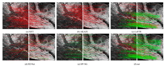
Figure 14.
Comparison of Matching Results for Images with Rotation Variations. Green: correct matches, error ≤ 3 pixels; red: incorrect matches, error > 3 pixels.
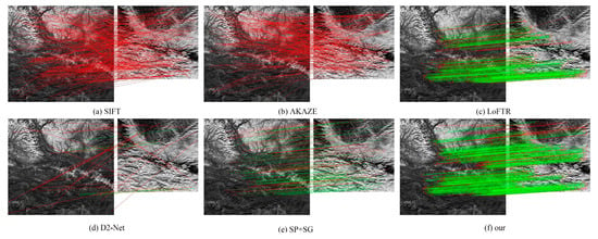
Figure 15.
Comparison of Image Matching Results under Scale Variations. Green: correct matches, error ≤ 3 pixels; red: incorrect matches, error > 3 pixels.
The SIFT and AKAZE algorithms relied on texture to extract keypoints and descriptors. However, the significant texture differences between infrared and visible images ultimately prevented effective matching points from being found in scenes with variations in angle and scale.
D2-Net showed limited robustness under rotation or resolution changes, as its fixed-scale feature maps constrained keypoint detection, leading to a substantial reduction in detected points.
SP + SG produced sparse outputs from grid detectors at lower resolutions, while angular changes reduced cosine similarity of shallow descriptors. Thus, although many valid matches were extracted, accuracy was lower than that of LoFTR and the proposed method.
Compared with LoFTR, the proposed model identified more valid matches under both rotation and scaling transformations. Other methods failed to correlate matching points between the two image sets due to significant differences in infrared and visible light textures across varying terrains, coupled with the nonlinear grayscale mapping of infrared band textures. The proposed model separates and extracts infrared and visible light features, enabling more effective extraction of the respective characteristics of the two image types. It demonstrated certain effectiveness in rotation and scale transformation tests.
3.5. Realistic Image Registration Experiment
Ensuring accurate image registration is one of the main objectives of matching infrared and visible images. To evaluate the performance of the proposed model, image registration experiments were conducted, and the results are presented in Figure 16. First, the homography matrix was estimated from the matching point sets generated by the proposed method. This visible image was mapped onto the infrared coordinate system to achieve spatial registration. The final images that were registered are overlaid in a grid layout of upper and lower layers. Figure 16 shows the overall registration result (left) and enlarged local area (right). The black areas are where the two images do not overlap. The registered images exhibit consistent textures and demonstrate precise alignment.
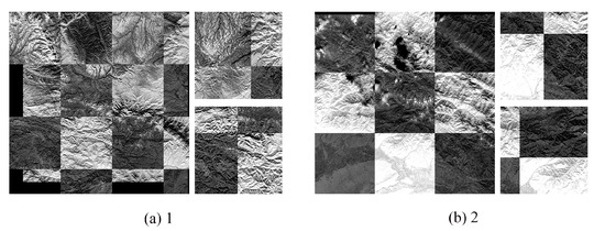
Figure 16.
The results of image registration using the method described in this paper.
4. Discussion and Conclusions
The primary objective of matching infrared and visible remote sensing images is to achieve spatial registration between these heterogeneous modalities. This establishes a reliable foundation for subsequent applications, including image fusion, feature analysis, and dynamic monitoring. Nevertheless, the underlying imaging principles of these two bands, visible and infrared, are intrinsically different, thus resulting in very different texture patterns. Non-linear discrepancies such as these are not efficiently captured by traditional schemes and, hence, have been challenging to handle. We propose EWAM, a physics-inspired dual-channel model based on a Transformer coarse-to-fine matching architecture. It employs two synergistic core modules to decouple features from different modalities. The Environment-Adaptive Radiation Feature Extractor employs a scene adaptive gating mechanism to compress global thermal statistics into learnable latent vectors, dynamically modulating feature propagation under radiometric fluctuations. Meanwhile, the Wavelet Transform High-Frequency Enhancement Module simultaneously utilizes learnable wavelet-based enhancement, covariance pooling, and directional perceptual losses to restore edges degraded by infrared point-spread blur and preserve second-order radiance correlations. By concurrently processing radiative statistics and spatial high-frequency structures, these modules collectively enhance feature robustness and discriminability in complex environments. The proposed method was compared against SIFT, AKAZE, D2-Net, SP + SG, and LoFTR across five scene categories: mountain, desert, gobi, city, and farmland. The proposed method achieved the highest accuracy rates across the five scenes, exceeding those of the best-performing baseline models by 2.7%, 2.6%, 2.0%, 2.3%, and 1.8%, while reducing the RMSE to 1.85 pixels. The results show that EWAM produced a larger number of matching points than the other methods, with a more uniform spatial distribution. Future work will focus on developing a lightweight version of the model to enable real-time processing, which is essential for large-scale remote sensing monitoring applications.
Author Contributions
Conceptualization, M.L. and H.T.; software, M.L. and H.T.; methodology, M.L. and H.T.; validation, M.L. and H.Z.; investigation, M.L. and H.Z.; data curation, M.L., H.Z. and J.C.; writing—original draft preparation, M.L.; writing—review and editing, M.L., H.T., H.Z. and J.C. All authors have read and agreed to the published version of the manuscript.
Funding
This research was funded by the National Civil Aerospace Preresearch Project (D040105) (Center Project No. BH2501). The APC was covered by the same grant.
Data Availability Statement
The Five-Billion-Pixels dataset https://doi.org/10.1016/j.isprsjprs.2023.03.009, Thermal Infrared and Multispectral Image Dataset https://doi.org/10.21227/Y32J-XG16 and Landsat 8 (Geospatial Data Cloud) are openly available as listed. Gaofen-7 data used in this study are subject to institutional restrictions; processed subsets are available from the corresponding author upon reasonable request, with permission from the data owner.
Conflicts of Interest
The authors declare no conflicts of interest.
Abbreviations
| SP + SG | SuperPoint + SuperGlue |
| RMSE | Root Mean Square Error |
| LH | Horizontal gradient sub-band |
| HL | Vertical gradient sub-band |
| HH | Diagonal gradient sub-band |
| DWT | Discrete Wavelet Transform |
| Db | Daubechies |
| Coif | Coiflet |
| DT-CWT | Dual-Tree Complex Wavelet Transform |
References
- Zhao, Q.; Yu, L.; Du, Z.; Peng, D.; Hao, P.; Zhang, Y.; Gong, P. An Overview of the Applications of Earth Observation Satellite Data: Impacts and Future Trends. Remote Sens. 2022, 14, 1863. [Google Scholar] [CrossRef]
- Li, J.; Wu, M.; Lin, L.; Yuan, Q.; Shen, H. GLCD-DA: Change Detection from Optical and SAR Imagery Using a Global-Local Network with Diversified Attention. ISPRS J. Photogramm. Remote Sens. 2025, 226, 396–414. [Google Scholar] [CrossRef]
- Zhang, B.; Chang, L.; Wang, Z.; Wang, L.; Ye, Q.; Stein, A. Multi-Decadal Dutch Coastal Dynamic Mapping with Multi-Source Remote Sensing Imagery. Int. J. Appl. Earth Obs. Geoinf. 2025, 138, 104452. [Google Scholar] [CrossRef]
- Xu, Q.; Zhao, B.; Dai, K.; Li, W.; Zhang, Y. Remote Sensing for Landslide Investigations: A Progress Report from China. Eng. Geol. 2023, 321, 107156. [Google Scholar] [CrossRef]
- Pu, R.; Landry, S.; Yu, Q. Object-Based Urban Detailed Land Cover Classification with High Spatial Resolution IKONOS Imagery. Int. J. Remote Sens. 2011, 32, 3285–3308. [Google Scholar] [CrossRef]
- Mozgeris, G.; Gadal, S.; Jonikavičius, D.; Straigytė, L.; Ouerghemmi, W. Hyperspectral and color-infrared imaging from ultralight aircraft: Potential to recognize tree species in urban environments. In Proceedings of the 2016 8th Workshop on Hyperspectral Image and Signal Processing: Evolution in Remote Sens (WHISPERS), Los Angeles, CA, USA, 21–24 August 2016; pp. 1–5. [Google Scholar] [CrossRef]
- Xu, K.; Yang, W.; Ye, H. Thermal infrared reflectance characteristics of natural leaves in 8–14 μm region: Mechanistic modeling and relationships with leaf water content. Remote Sens. Environ. 2023, 294, 113631. [Google Scholar] [CrossRef]
- Teng, Y.; Ren, H.; Hu, Y.; Dou, C. Land surface temperature retrieval from SDGSAT-1 thermal infrared spectrometer images: Algorithm and validation. Remote Sens. Environ. 2024, 315, 114412. [Google Scholar] [CrossRef]
- Li, Y.; Dang, B.; Zhang, Y.; Liu, Z.; Wang, X. Water Body Classification from High-Resolution Optical Remote Sensing Imagery: Achievements and Perspectives. ISPRS J. Photogramm. Remote Sens. 2022, 187, 306–327. [Google Scholar] [CrossRef]
- Cheng, F.; Zhou, Y.; Huang, X.; Huang, R.; Tai, Y.; Shi, J. CycleRegNet: A scale-aware and geometry-consistent cycle adversarial model for infrared and visible image registration. Measurement 2025, 242, 116063. [Google Scholar] [CrossRef]
- Yang, Y.; Liu, S.; Zhang, H.; Li, D.; Ma, L. Multi-Modal Remote Sensing Image Registration Method Combining Scale-Invariant Feature Transform with Co-Occurrence Filter and Histogram of Oriented Gradients Features. Remote Sens. 2025, 17, 2246. [Google Scholar] [CrossRef]
- Zhu, B.; Yang, C.; Dai, J.; Li, H.; Wang, Q. R2FD2: Fast and Robust Matching of Multimodal Remote Sensing Images via Repeatable Feature Detector and Rotation-Invariant Feature Descriptor. IEEE Trans. Geosci. Remote Sens. 2023, 61, 1–15. [Google Scholar] [CrossRef]
- Li, J.; Bi, G.; Wang, X.; Nie, T.; Huang, L. Radiation-Variation Insensitive Coarse-to-Fine Image Registration for Infrared and Visible Remote Sensing Based on Zero-Shot Learning. Remote Sens. 2024, 16, 214. [Google Scholar] [CrossRef]
- Le Moigne, J. Introduction to remote sensing image registration. In Proceedings of the 2017 IEEE International Geoscience and Remote Sensing Symposium (IGARSS), Fort Worth, TX, USA, 23–28 July 2017; pp. 2565–2568. [Google Scholar] [CrossRef]
- Lowe, D.G. Distinctive image features from scale-invariant keypoints. Int. J. Comput. Vis. 2004, 60, 91–110. [Google Scholar] [CrossRef]
- Rublee, E.; Rabaud, V.; Konolige, K.; Bradski, G. ORB: An efficient alternative to SIFT or SURF. In Proceedings of the 2011 International Conference on Computer Vision (ICCV), Barcelona, Spain, 6–13 November 2011; pp. 2564–2571. [Google Scholar] [CrossRef]
- Alcantarilla, P.; Nuevo, J.; Bartoli, A. Fast explicit diffusion for accelerated features in nonlinear scale spaces. In Proceedings of the British Machine Vision Conference 2013, Bristol, UK, 9–13 September 2013; pp. 13.1–13.11. [Google Scholar] [CrossRef]
- Dai, J.; Song, W.; Li, Y. Progressive SIFT matching algorithm for multi-source optical satellite images. Acta Geod. Cartogr. Sin. 2014, 43, 746–752. [Google Scholar] [CrossRef]
- Xiang, Y.; Wang, F.; You, H. OS-SIFT: A robust SIFT-like algorithm for high-resolution optical-to-SAR image registration in suburban areas. IEEE Trans. Geosci. Remote Sens. 2018, 56, 3078–3090. [Google Scholar] [CrossRef]
- Xi, S.; Li, W.; Xie, J.; Mo, F. Feature point matching between infrared image and visible light image based on SIFT and ORB operators. Infrared Technol. 2020, 42, 168–175. [Google Scholar] [CrossRef]
- Bai, Y. Research of Image Detection and Matching Algorithms. Appl. Comput. Eng. 2023, 5, 519–526. [Google Scholar] [CrossRef]
- Wang, Z.; Li, Z.; Cheng, L.; Yan, G. An improved ORB feature extraction and matching algorithm based on affine transformation. In Proceedings of the 2020 Chinese Automation Congress (CAC), Shanghai, China, 6–8 November 2020; pp. 1511–1515. [Google Scholar] [CrossRef]
- Tang, Y.; Wang, Z.; Zhang, Z. Registration of sand dune images using an improved SIFT and SURF algorithm. J. Tsinghua Univ. (Sci. Technol.) 2020, 61, 161–169. [Google Scholar] [CrossRef]
- Wang, H.; Li, A.; Ye, Q.; Zhu, X.; Song, L.; Ji, Y. A coarse-to-fine heterologous registration method for infrared-visible images based on MDC and MSMA-SCW descriptors. Opt. Lasers Eng. 2025, 190, 108955. [Google Scholar] [CrossRef]
- Barroso-Laguna, A.; Mikolajczyk, K. Key.net: Keypoint detection by handcrafted and learned CNN filters revisited. IEEE Trans. Pattern Anal. Mach. Intell. 2023, 45, 698–711. [Google Scholar] [CrossRef]
- Han, X.; Leung, T.; Jia, Y.; Sukthankar, R.; Berg, A.C. MatchNet: Unifying Feature and Metric Learning for Patch-Based Matching. In Proceedings of the IEEE Conference on Computer Vision and Pattern Recognition (CVPR), Boston, MA, USA, 7–12 June 2015; pp. 3279–3286. [Google Scholar] [CrossRef]
- Deng, Y.; Zhang, K.; Zhang, S.; Li, Y.; Ma, J. ResMatch: Residual attention learning for feature matching. In Proceedings of the AAAI Conference on Artificial Intelligence, Vancouver, BC, Canada, 20–27 February 2024; pp. 1501–1509. [Google Scholar] [CrossRef]
- DeTone, D.; Malisiewicz, T.; Rabinovich, A. SuperPoint: Self-Supervised Interest Point Detection and Description. In Proceedings of the IEEE Conference on Computer Vision and Pattern Recognition Workshops, Salt Lake City, UT, USA, 18–22 June 2018; pp. 224–236. [Google Scholar] [CrossRef]
- Sarlin, P.-E.; DeTone, D.; Malisiewicz, T.; Rabinovich, A. SuperGlue: Learning feature matching with graph neural networks. In Proceedings of the 2020 IEEE/CVF Conference on Computer Vision and Pattern Recognition (CVPR), Seattle, WA, USA, 14–19 June 2020; pp. 4937–4946. [Google Scholar] [CrossRef]
- Sun, J.; Shen, Z.; Wang, Y.; Bao, H.; Zhou, X. LoFTR: Detector-free local feature matching with transformers. In Proceedings of the 2021 IEEE/CVF Conference on Computer Vision and Pattern Recognition (CVPR), Nashville, TN, USA, 20–25 June 2021; pp. 8918–8927. [Google Scholar] [CrossRef]
- Vaswani, A.; Shazeer, N.; Parmar, N.; Uszkoreit, J.; Jones, L.; Gomez, A.N.; Kaiser, L.; Polosukhin, I. Attention is all you need. In Advances in Neural Information Processing Systems 30 (NIPS 2017); Curran Associates, Inc.: Red Hook, NY, USA, 2017; pp. 5998–6008. [Google Scholar] [CrossRef]
- Li, H.; Yang, Z.; Zhang, Y.; Jia, W.; Yu, Z.; Liu, Y. MulFS-CAP: Multimodal fusion-supervised cross-modality alignment perception for unregistered infrared-visible image fusion. IEEE Trans. Pattern Anal. Mach. Intell. 2025, 47, 3673–3690. [Google Scholar] [CrossRef] [PubMed]
- Bala, R.; Prasad, R.; Yadav, V.P.; Sharma, J. A comparative study of land surface temperature with different indices on heterogeneous land cover using Landsat 8 data. Int. Arch. Photogramm. Remote Sens. Spatial Inf. Sci. 2018, XLII-5, 389–394. [Google Scholar] [CrossRef]
- Bian, Z.; Liu, X.; Li, A.; Zhang, X.; Chen, Y.; Tang, L. Retrieval of Leaf, Sunlit Soil, and Shaded Soil Component Temperatures Using Airborne Thermal Infrared Multiangle Observations. IEEE Trans. Geosci. Remote Sens. 2016, 54, 4660–4671. [Google Scholar] [CrossRef]
- Asner, G.P.; Heidebrecht, K.B. Spectral unmixing of vegetation, soil and dry carbon cover in arid regions: Comparing multi-spectral and hyperspectral observations. Int. J. Remote Sens. 2002, 23, 3939–3958. [Google Scholar] [CrossRef]
- Daubechies, I. Orthonormal bases of compactly supported wavelets. Commun. Pure Appl. Math. 1988, 41, 909–996. [Google Scholar] [CrossRef]
- Li, J.; Zhang, S.; Sun, Y.; Han, Q.; Sun, Y.; Wang, Y. Frequency-Driven Edge Guidance Network for Semantic Segmentation of Remote Sensing Images. IEEE J. Sel. Top. Appl. Earth Obs. Remote Sens. 2024, 17, 9677–9693. [Google Scholar] [CrossRef]
- Evers, J.; Evers, F.; Goppelt, F.; Schmidt-Vollus, R. Singular spectrum analysis-based image sub-band decomposition filter banks. EURASIP J. Adv. Signal Process. 2020, 2020, 29. [Google Scholar] [CrossRef]
- González-Audícana, M.; Otazu, X.; Fors, O.; Seco, A. Comparison between Mallat’s and the ‘à trous’ discrete wavelet transform based algorithms for the fusion of multispectral and panchromatic images. Int. J. Remote Sens. 2005, 26, 595–614. [Google Scholar] [CrossRef]
- Shi, W.; Zhu, C.; Tian, Y.; Nichol, J. Wavelet-based image fusion and quality assessment. Int. J. Appl. Earth Obs. Geoinf. 2005, 6, 241–251. [Google Scholar] [CrossRef]
- Tong, X.; Xia, G.; Zhu, X. Enabling country-scale land cover mapping with meter-resolution satellite imagery. ISPRS J. Photogramm. Remote Sens. 2023, 196, 178–196. [Google Scholar] [CrossRef] [PubMed]
- Kedar, S. Thermal Infrared and Multispectral Image Dataset. IEEE DataPort, 18 June 2021. [Google Scholar] [CrossRef]
Disclaimer/Publisher’s Note: The statements, opinions and data contained in all publications are solely those of the individual author(s) and contributor(s) and not of MDPI and/or the editor(s). MDPI and/or the editor(s) disclaim responsibility for any injury to people or property resulting from any ideas, methods, instructions or products referred to in the content. |
© 2025 by the authors. Licensee MDPI, Basel, Switzerland. This article is an open access article distributed under the terms and conditions of the Creative Commons Attribution (CC BY) license (https://creativecommons.org/licenses/by/4.0/).