Highlights
What are the main findings?
- A ResNet-50-based deep learning framework (ResNet-IST) was successfully developed to integrate spectral and spatial features from satellite imagery for the precise detection and classification of wildfire-affected vegetation.
- When evaluated across ten global sites, the ResNet-IST model demonstrated superior performance in identifying burned areas compared to the established VASTI and NBR indices.
What is the implication of the main finding?
- It introduces a superior, intelligent method for global environmental monitoring. The ResNet-IST model represents a paradigm shift from traditional, fixed-formula indices to an adaptive deep learning approach, enabling more accurate and reliable detection of burned vegetation on a global scale.
- It enables more effective disaster assessment and ecological recovery. By significantly improving detection accuracy over current methods (VASTI and NBR), the model provides crucial data for precise post-fire evaluation, which is fundamental for coordinating restoration efforts and managing ecosystem health.
Abstract
Timely and accurate detection of burned areas is crucial for assessing fire damage and contributing to ecosystem recovery efforts. In this study, we propose a framework for detecting fire-affected vegetation anomalies on the basis of a ResNet deep learning (DL) algorithm by merging spectral and textural features (ResNet-IST) and the vegetation abnormal spectral texture index (VASTI). To train the ResNet-IST, a vegetation anomaly dataset was constructed on high-resolution 30 m fire-affected remote sensing images selected from the Global Fire Atlas (GFA) to extract the spectral and textural features. We tested the model to detect fire-affected vegetation in ten study areas across four continents. The experimental results demonstrated that the ResNet-IST outperformed the VASTI by approximately 3% in terms of anomaly detection accuracy and achieved a 5–15% improvement in the detection of the normalized burn ratio (NBR). Furthermore, the accuracy of the VASTI was significantly greater than that of NBR for burn detection, indicating that the merging of spectral and textural features provides complementary advantages, leading to stronger classification performance than the use of SFs alone. Our results suggest that deep learning outperforms traditional mathematical models in burned vegetation anomaly detection tasks. Nevertheless, the scope and applicability of this study are somewhat limited, which also provides directions for future research.
1. Introduction
Forests are intricate ecosystems that serve as habitats for countless species. These natural environments are integral to maintaining the balance of the Earth’s systems, providing numerous benefits such as regulating atmospheric conditions, enhancing the economy, and ensuring the quality of life for people [1,2]. Wildfires, as major natural disasters, are among the most challenging disturbances faced by forests and can lead to the destruction of biomass and biodiversity, changes in continuous patterns of vegetation, and severe threats to society, the economy, and even human life [3,4,5]. Therefore, more studies should aim at accurately detecting fire-damaged vegetation for fire response strategies, guiding effective restoration efforts, and even preventing deadly threats [6,7]. The use of remote sensing for forest fire detection and mapping originated in the 1960s, setting the stage for its subsequent development in fire monitoring [8]. With the advancement of satellite imaging technology, an increasing amount of remote sensing data has since been used for fire detection and burn scar mapping, thus reducing labor and resource costs of studying vegetation fires and offering an efficient and accurate research approach [5,9,10].
Satellite spectral indices are the most commonly used methods for detecting burned areas. These spectral indices can effectively represent different plant health conditions and reflect the impact of fires, which rely on the loss of vegetation caused by various disturbances [11]. Specifically, two main categories of spectral indices are useful for identifying burned vegetation: vegetation indices (VIs) and fire indices (FIs). Since forest fires can cause vegetation changes, the differences between normal and anomalous areas can be distinguished by several VIs, such as the normalized difference vegetation index (NDVI) [12,13], the enhanced vegetation index (EVI) [14], and the global environmental monitoring index (GEMI) [15,16], among others. In recent years, remarkable results have been produced in vegetation damage detection using VIs [17]. The development of numerous FIs has been driven by dramatic shifts in reflectance values from the near-infrared (NIR) to shortwave infrared (SWIR) bands. Theoretically, the normalized burn ratio (NBR) [18], the normalized difference SWIR (NDSWIR) [19], and the burning area index (BAI) [20] were specifically proposed to detect burned areas. However, although spectral indices have been proven to be capable of detecting burned areas, spectral information limitations frequently cause confusion at the boundaries of fire-affected areas, increasing the susceptibility of these indices to misclassification. These shortcomings limit their robustness and generalizability across diverse ecosystems. Furthermore, many existing studies have overlooked the relationship between spatial information and forest fires.
Texture features (TFs) within the two-dimensional spatial attributes of satellite images contain the variation in burned vegetation. TFs describe the spatial relationship between the central pixel and surrounding pixels, reflecting the appearance characteristics of fire-affected vegetation in imagery, such as texture, color, and shape. In recent years, several researchers have proposed enhancing satellite classification capabilities by incorporating spatial TFs [21,22]. For example, Mitri and Gitas introduced a novel model that utilized a semiautomatic object-oriented method for fire-affected plants [23]. This model incorporates TFs to differentiate regions with comparable spectral values, helping to minimize spectral overlap between various objects. Shama et al. utilized polarization and TFs from Sentinel-1A images to extract burned areas [24]. They integrated multiple changes in SAR features resulting from forest fires into a random forest (RF) model. The results showed high agreement, with an accuracy of 87.12%, a commission error of 20.44%, and an omission error of 12.88%. These studies show that the use of spatial features to detect burned vegetation is feasible, but the combination of spectral features (SFs) and TFs has not been given much consideration. Therefore, we conducted comparative tests on SFs and TFs, selecting several with high separability for explicit integration, resulting in the development of the vegetation abnormal spectral texture index (VASTI). The results indicate that VASTI significantly improves the accuracy of burned vegetation extraction compared with the use of SFs or TFs alone [25]. Nevertheless, as a purely mathematical model, VASTI lacks the capacity to capture nonlinear interactions between features and remains constrained in terms of generalization across different fire intensities and vegetation types. This limitation underscores the need for more advanced approaches capable of learning complex spectral–textural relationships. Therefore, to address the limitations of studies that rely solely on SFs, TFs, or their explicit combinations, we propose the introduction of a deep learning (DL) approach at the forefront of current research. Specifically, we develop a DL–based feature integration model that harnesses the advantages of contemporary algorithms to transcend the inherent shortcomings of conventional feature fusion techniques.
Recently, DL approaches have seen considerable progress, becoming highly effective and accurate solutions for various computer vision challenges, such as classifying images [26,27,28], semantic segmentation [29,30,31], and target detection [32,33]. Various deep neural networks (DNNs) have been proposed. DNNs can be categorized into three types: feed-forward deep networks (FFDNs) [34,35], feed-back deep networks (FBDNs) [36,37], and bi-directional deep networks (BDDNs) [38,39]. Among these, ResNet, a well-established and widely used convolutional neural network (CNN) architecture, was introduced by He et al., effectively addresses the issues of vanishing and exploding gradients that are common in traditional network structures [32]. Its efficiency is further enhanced by its minimal parameterization and the use of basic backpropagation to reduce computational costs. It leverages a deep residual learning architecture that increases network depth by employing multiple residual blocks and allows model layers to learn residual functions concerning the layer inputs. ResNets improve upon traditional neural networks by using skip connections, making them significantly smaller than conventional CNNs while maintaining comparable performance, effectively solving the problem of gradient vanishing or exploding [40]. Owing to these advantages, deep residual learning has been demonstrated to be a powerful instrument in various remote sensing applications. In particular, ResNet has been introduced for high-resolution satellite imagery classification tasks and has achieved excellent accuracy [41,42,43]. ResNet also shows great potential in anomaly detection for forest fires. For example, Zhang et al. proposed a transfer learning-based FT-ResNet50 model, which was first trained on ImageNet and then tailored for forest fire detection using UAV-based imagery [44]. By fine-tuning the model to the unique features of the forest fire dataset, the FT-ResNet50 model was enhanced to better capture deep semantic features from fire images, improving its efficiency in the process. This finding demonstrates that FT-ResNet50 delivers excellent accuracy in forest fire detection tasks. In addition, numerous studies have demonstrated that ResNet has achieved a series of breakthroughs in fire detection tasks and has the ability to identify abnormal vegetation accurately [45,46,47]. Nevertheless, limited attention has been given to utilizing ResNet in combination with spectral and texture features for the abnormal monitoring of fire-affected forests.
In this study, we specifically propose the ResNet-IST model, which is a deep ResNet50-based, combined spectral and textural feature method for detecting anomalous burned vegetation areas. Our primary objectives are to (1) develop a DL framework based on ResNet50 (ResNet-IST) to extract spectral and spatial information from satellite images of normal and abnormal vegetation samples and perform feature fusion. This model is then employed to detect and classify abnormal vegetation areas affected by wildfires. (2) The performance of the ResNet-IST framework is evaluated on the basis of abnormal detection results across study areas from ten sites worldwide, and its performance is compared with that of other burned area detection indices, the VASTI and NBR.
2. Study Area and Data
2.1. Satellite Dataset of Anomalous Vegetation
Based on the 2016 fire point information from the Global Fire Atlas (GFA) [48], we selected ten research locations worldwide, each representing one of six distinct landcover types, to construct a burned vegetation dataset. The selected sites were chosen to cover diverse climatic zones and vegetation types while ensuring clear fire boundaries and minimal cloud interference, thereby maximizing representativeness and data quality. The images in this dataset were captured by the Landsat-8 satellite, which has a thermal infrared sensor (TIRS) and an operational land imager (OLI) [49]. The Landsat-8 OLI images employed in this research were retrieved from the official platform of the U.S. Geological Survey (USGS) (https://earthexplorer.usgs.gov/ (accessed on 18 July 2023)). Figure 1 displays the locations of these sites. We meticulously identified and annotated the burned regions at each site, creating a detailed dataset consisting of 1772 samples. This dataset comprises 3554 images, with each sample consisting of two optical images at a 30 m resolution taken before and after the fire events in the same regions. Detailed information about the ten study locations, including names, coordinates, land cover types, and sample sizes, is provided in Table 1. It should be noted that the number of samples varies across sites, reflecting differences in fire size and image quality. For instance, smaller fires or areas with cloud contamination yielded fewer valid samples (e.g., site (h), 29), whereas larger and clearer events provided more samples (e.g., site (j), 267). The dataset was constructed to compare the variations in the spectral and textural features before and after the fire disturbance, aiming to identify features appropriate for constructing a new index. To verify the effectiveness of the novel index, its accuracy and performance were tested through a representative subset of samples from each site.
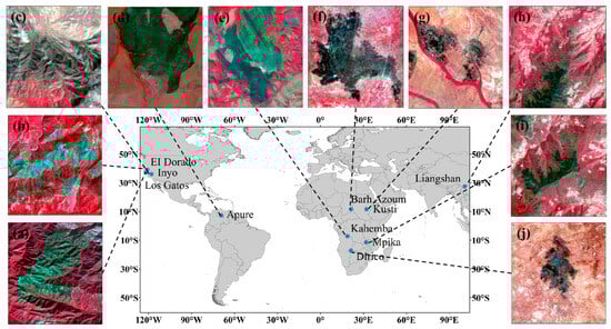
Figure 1.
Distribution of the sample sites in the burned vegetation dataset. Ten study area images showing bands 5, 4, and 3 false color combinations from Landsat 8: (a) Los Gatos, (b) EI Dorado, (c) Inyo, (d) Apure, (e) Kahemba, (f) Barh Azoum, (g) Kusti, (h) Liangshan, (i) Mpika, and (j) Dirico.

Table 1.
Summary of the selected sites in this study. The sites’ names, longitudes (lon), latitudes (lat), land cover types, number of samples, and sample size were included.
2.2. Data Processing
This study selected ten globally distributed sites suitable for postfire burn scar extraction research using fire point information provided by the GFA, which includes fire occurrence and end times, affected areas, and fire point coordinates. The site selection criteria included minimal cloud cover and clear anomaly boundaries to ensure the accuracy of model training. The site selection aimed to capture a representative range of ecosystems and fire scenarios while ensuring clear anomaly boundaries and minimal cloud contamination. For each site, bi-temporal remote sensing images were collected, capturing both pre-fire and post-fire conditions, and the fire-affected areas were identified through visual interpretation. The images and their corresponding labels were then divided into 200 × 200 pixel segments. Each segment was assessed, and those with more than 80% mask coverage were designated as abnormal vegetation samples, contributing to a database for abnormal vegetation. Moreover, we established a matching normal vegetation database for each abnormal segment using the pre-fire images. This auxiliary dataset enabled us to calculate the changes in TFs following a wildfire and identify those with significant discriminatory power.
The processes of selecting normal and abnormal vegetation samples, image analysis, anomaly identification, and database creation form the initial stage of our data processing workflow. This step is essential, as the effectiveness of data processing significantly influences the performance of the dataset in subsequent research. In future studies, this dataset will be used primarily to investigate changes in texture and spectral properties before and after fire events, with the aim of identifying the most distinguishable features in both domains. These features will then be used to construct composite indices and extract and validate vegetation burn areas.
3. Methodology
3.1. ResNet-IST Framework
Our ResNet-based merged SFs and TFs (ResNet-IST) framework was designed to extract different kinds of image features using a deep residual convolutional network ResNet50 algorithm (Figure 2). First, Landsat images at a 30 m spatial resolution were selected to construct a dataset comprising two classes of samples: normal vegetation and abnormal vegetation, 70% of which were used for model training and 30% for testing. Second, this study utilizes a ResNet50-based framework that integrates SFs, TFs, and VASTI to learn and train the characteristics of normal and abnormal vegetation samples. Third, after network construction, we applied fire-affected anomaly forest detection in ten study areas of different sites via ResNet-IST and the comparable models VASTI and NBR. Finally, we conducted a visual evaluation and accuracy calculation on the results of the ResNet-IST model, comparing them with those obtained from VASTI and the widely used NBR index. The findings highlighted that the application of the DL method notably enhances the accuracy in identifying areas impacted by fire.
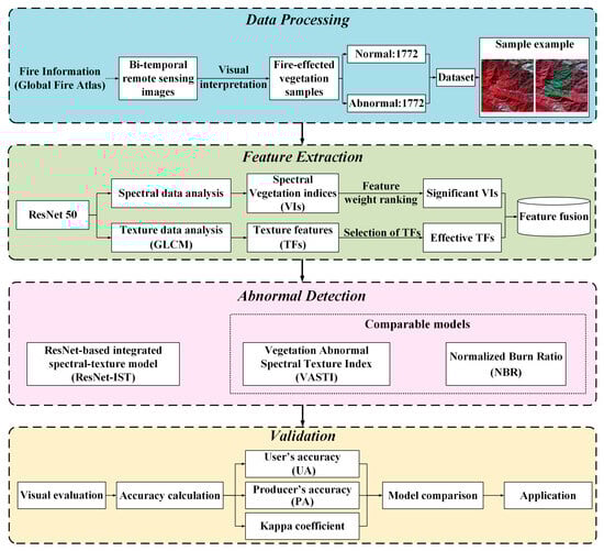
Figure 2.
Architectural framework and procedures of this research. It is generally divided into four parts: data processing, feature input, modeling, verification, and application.
3.2. Extraction of the Input Features
This study uses the ResNet50 network to identify and classify burned vegetation regions in remote sensing images. In DL models, the input features are crucial for classification accuracy and performance [50]. Therefore, effectively integrating these features is highly important. In this study, three types of features are used for ResNet50: 12 SFs, which represent various SFs; 9 TFs; and a combined spectral-texture index, VASTI. When extracting TFs, factors such as the gray level, step size, window size, and direction of the gray-level co-occurrence matrix (GLCM) need to be considered. Each type of feature is described below.
3.2.1. Spectral Indices
VIs are crucial measures obtained from spectral reflectance data by combining multiple wavelengths that correspond to the biophysical characteristics of vegetation, which can reflect different types of information on the basis of variations in the spectral data from remote sensing imagery [51]. These indices are extensively utilized in vegetation studies to evaluate different aspects, such as health conditions, growth dynamics, and coverage extent. Numerous studies have demonstrated that VIs are also effective in identifying anomalous vegetation [52]. Based on previous research, this study selects 12 VIs as spectral input features for the ResNet-IST model. The detailed information of the twelve VIs are shown in Table 2.
Table 2.
Details for the 12 vegetation indices, including the name, formula, and the references.
3.2.2. Texture Features
Texture is a visual characteristic that reflects homogeneity in an image, which is expressed through the distribution of pixel intensities and their surrounding spatial neighborhoods [64]. Unlike SFs, TFs are not influenced by reflectance changes and instead focus on representing the spatial relationships between the central pixel and its neighboring pixels [65]. This study employs the statistical technique of GLCM calculation to obtain the TFs of different samples. This method, introduced by Haralick et al. in the early 1970s, is a widely used approach in texture analysis [66]. The core idea is to quantify the frequency of different pixel pair combinations. To quantify and describe these TFs, statistical attributes are computed from the GLCM [67]. The GLCM can be calculated as follows:
where d represents the relative distance of the pixel count, which corresponds to the step size; ω denotes the co-occurrence direction, with values of 0°, 45°, 90°, and 135°; # represents the set; and (x, y) refers to the coordinates of the pixels, with L representing gray levels in the image.
However, while the GLCM provides information about the direction, distance, and variation in pixel intensities, it does not directly distinguish TFs. Ultimately, we selected nine commonly used TFs as inputs for the model, and the formulas of these TFs are shown in Table 3.
Table 3.
The formulas for the nine textures.
3.2.3. Vegetation Anomaly Spectral Texture Index
To achieve a complementary advantage between SFs and TFs, we previously proposed an integrated index VASTI. This index applies the principle of maximizing differences, explicitly combining SFs and TFs that have a high discriminative ability between normal and anomalous vegetation, using a specific calculation formula [25]. In the present study, VASTI plays a dual role with clearly separated protocols: (i) as one input channel among all spectral–textural features to provide a compact, physics-based prior for ResNet-IST; and (ii) as an independent benchmark computed strictly following its original formulation in [25], without any learning components. Although VASTI has demonstrated a significant improvement in fire-affected anomaly detection accuracy compared with the use of either SFs or TFs alone, the purely mathematical model still has certain limitations. These include computational constraints and the challenges of feature selection attribution, which hinder the generalizability and robustness of the model. Accordingly, using VASTI both as an input and as a standalone comparator is intended to quantify the incremental benefit brought by deep learning over the physical index, while avoiding methodological circularity by ensuring that the benchmark is evaluated independently from the network.
The VASTI is a comprehensive index that integrates the VIs GEMI and EVI with the texture index Auto_cor and is composed of the VASI and VATI. The calculation process is as follows:
This index uses the concept of amplified difference, leveraging the spectral and pixel value differences between normal and anomalous vegetation to maximize their distinction, thereby improving the differentiation between the two vegetation states. Therefore, integrating TFs with SFs can effectively compensate for the shortcomings of SFs while accounting for the spatial characteristics of the images, thus increasing the accuracy of identifying anomalous vegetation [68].
3.3. ResNet Algorithm
ResNet represents a breakthrough in CNN architecture, effectively resolving the common problems of vanishing and exploding gradients. This framework was first introduced during the 2015 ImageNet Large Scale Visual Recognition Challenge (ILSVRC), enabling the successful training of much deeper models [28]. Owing to its outstanding performance, ResNet has achieved leading results in several computer vision challenges and has been widely implemented across various tasks, including image classification [69,70], object detection [71,72], and semantic segmentation [73,74]. In ResNet, the initial input is directly linked to the next layer of neurons, reducing the residual (difference) between the input and the output. When the input x is passed directly to the output of the network, the learning objective is adjusted, as expressed by:
where is the final output, x is the original input, and is the expected output. The core innovation of ResNet lies in its residual blocks, which serve as the fundamental building units of the entire network. The residual blocks optimize the network architecture, requiring fewer parameter adjustments, enabling quicker training, and achieving performance that surpasses human capabilities. Figure 3 shows the principle of residual learning in ResNet. A residual block primarily consists of two components: one or more convolutional layers and a shortcut connection. The residual structures are divided into two types: Figure 3a is optimized for networks with fewer layers, such as ResNet18 and ResNet34, whereas the structure shown in Figure 3b is tailored for deeper models such as ResNet50, ResNet101, and ResNet152, as it reduces the number of parameters and computational demands [28].
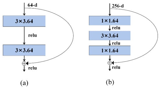
Figure 3.
Schematic diagram of two types of residual blocks. (a) is the residual block of networks with fewer layers such as ResNet18 and ResNet34; (b) is the residual block of deeper models such as ResNet50, ResNet101, and ResNet152.
Ultimately, we selected ResNet50 to serve as the core network in our model to extract various types of spectral and textural information from forest fire images (Table 4). The ResNet-50 framework consists of 49 convolutional layers, including a 3 × 3 convolution, along with an average pooling layer and a fully connected layer. This typical ResNet-50 setup has a total of 25.56 million parameters. In the “bottle-neck” block, each convolution is followed by a ReLU activation function and batch normalization. At the final fully connected layer, the Softmax function is employed for classification. ResNet-50 was specifically chosen over lighter versions such as ResNet-18 because its deeper architecture and additional residual blocks enable more comprehensive hierarchical feature extraction, which is crucial for capturing subtle spectral and textural differences between normal and burned vegetation that may be missed by shallower networks. While ResNet-50 has more parameters than ResNet-18, it maintains a reasonable balance between representational capacity and computational efficiency, ensuring robust performance in detecting anomalous vegetation without incurring prohibitive training costs.
Table 4.
The network configuration of ResNet50.
Figure 4 illustrates the workflow of the ResNet-IST model for identifying abnormal vegetation. Initially, normal and abnormal vegetation samples are fed into a pre-trained ResNet architecture. In this study, we adopted a leave-one-site-out cross-validation (LOSO-CV) strategy for model training and evaluation. Specifically, in each iteration, the data from one site were entirely reserved as the validation set, while the remaining nine sites were used for model training, allowing us to rigorously assess the model’s generalization capability on independent sites. This approach effectively prevents information leakage from the training data and provides a strict evaluation across spatially heterogeneous regions. Furthermore, to evaluate the spatial performance of the model, a representative sample from the held-out site was selected in each iteration for spatial mapping and accuracy assessment, thereby verifying the model’s predictive accuracy in unseen areas. This strategy ensures both the independence of training and validation and a comprehensive assessment of the model’s robustness in detecting anomalous vegetation across diverse geographic locations. The model leverages its convolutional layers, enhanced with residual connections, to extract deep and hierarchical features from the input samples. Subsequently, these features undergo dimensionality reduction and aggregation in the pooling layers. The pooled features are then mapped to the classification space through a series of fully connected layers. During the training, we adopted the Adam optimizer with an initial learning rate of 0.001. To ensure stable and efficient learning, we implemented a learning rate decay strategy, reducing the learning rate to 10% of its original value every 10 epochs. The batch size was set to 32 to balance computation efficiency and model performance. To prevent overfitting, we incorporated Dropout layers within the network architecture and applied L2 regularization to the model’s weights. Additionally, an early stopping strategy was employed to halt training when the validation loss no longer decreased, thus avoiding unnecessary computation and potential overfitting. After computing the loss function, the model’s parameters are updated based on the gradients obtained through backpropagation. Once training is complete, the model is deployed to identify regions of abnormal vegetation in new samples. The accuracy of the detection results is then evaluated to assess the model’s performance.
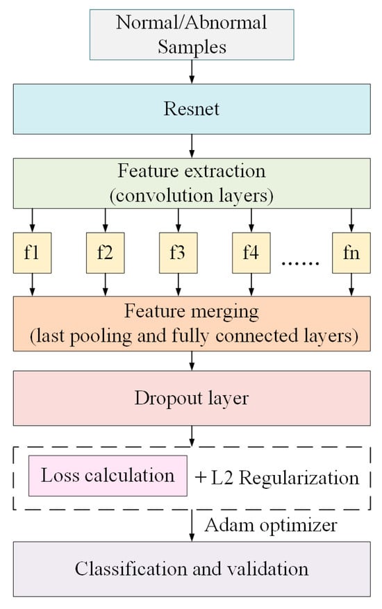
Figure 4.
Block diagram of the progress of the ResNet-IST model.
3.4. Comparison of the Normalized Burn Ratio Index
To compare the performance of the VASTI and ResNet-IST models in extracting anomalous vegetation, this study separately calculates the NBR for the extraction results of burned vegetation regions. The extraction results of these three methods in the study area are then validated and comparatively evaluated for accuracy.
The NBR is a commonly used index that helps identify areas where vegetation has changed due to fire disturbances [18]. By computing the ratio of the NIR to SWIR bands, the distinctive features of burned regions can be strengthened. By definition, the NBR highlights burned areas following a fire. The equation of NBR incorporates measurements of NIR and SWIR wavelengths: healthy vegetation exhibits high reflectance in the NIR spectrum, whereas recently burned areas show high reflectance in the SWIR spectrum. The calculation formula for NBR is as follows:
where represents the reflectance of the near-infrared band and where represents the reflectance of the shortwave infrared band.
NBR was selected as a baseline index because of its simplicity, widespread use, and proven effectiveness in burned area detection. However, it is acknowledged that NBR does not fully represent the spectrum of traditional mathematical models, and its role in this study is to provide a reference benchmark for evaluating improvements achieved by the proposed method.
3.5. Evaluation Method
We employed confusion matrices to verify the detection precision for diverse abnormal vegetation areas. Eventually, three evaluation metrics—user accuracy (UA), producer’s accuracy (PA), and the kappa coefficient—were chosen to provide a thorough assessment of the accuracy in extracting data from the different indices. The calculation methods for these metrics are outlined below:
where
3.6. Deep Learning Model Interpretability Analysis
In this study, to elucidate the impact of different spectral and texture features on the ResNet-IST model, we employed SHAP (SHapley Additive exPlanations) [75] values to determine the predictive contribution of each input feature. The SHAP value, originating from cooperative game theory [76], aims to fairly allocate the overall outcome based on the marginal contributions of individual participants within a collaborative process. In recent years, SHAP values have been introduced into the field of machine learning as an effective model interpretability method, enabling the decomposition of complex black-box model predictions into the sum of contributions from individual features [77]. This approach not only possesses theoretical advantages such as efficiency, fairness, nullity, and additivity but also provides a solid theoretical foundation for enhancing model transparency.
For a given sample , its features are denoted as . The model’s predicted value for this sample is , while the baseline value of the model (typically the mean of the target variable across all samples) is represented as . The relationship among these variables can be expressed as:
where is the SHAP value of . The calculation of SHAP values can be implemented using Python Version 3.14.0 (https://www.python.org/).
4. Results
4.1. Parameters Setting of GLCM
It is necessary to preprocess the spectral and texture features of the samples before constructing the ResNet-IST model. While the calculation of SFs is relatively straightforward, the computation of TFs requires careful consideration of the parameter settings for the GLCM. GLCM involves four parameters: orientation, displacement (distance), sliding window size, and gray levels. Variations in these parameters can significantly influence the resulting texture features. To minimize uncertainties arising from parameter selection, we conducted comparative experiments to determine the optimal GLCM settings for vegetation anomaly detection. Given that vegetation anomalies often manifest as subtle changes without consistent horizontal or vertical patterns, we fixed the displacement to 1 and averaged the GLCM calculations across four directions (0°, 45°, 90°, and 135°) to capture comprehensive spatial relationships. Commonly used gray levels in GLCM computations are 16, 32, 64, 128, and 256. With the displacement and directional averaging fixed, we initially employed a 3 × 3 window size to assess the impact of varying gray levels. As depicted in Figure 5a, the highest accuracy was achieved with a gray level of 64. Subsequently, fixing the gray level at 64, we evaluated different window sizes. Figure 5b indicates that a 7 × 7 window size yielded the highest overall accuracy.
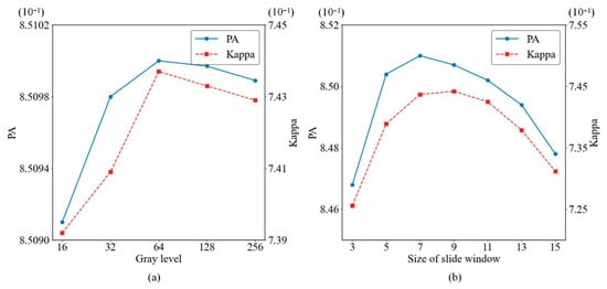
Figure 5.
Comparison of GLCM parameter settings: sliding window size and gray-level configuration. The left ordinate indicates the producer accuracy (PA), while the right ordinate displays the corresponding kappa coefficient. Panel (a) illustrates these trends of PA and kappa coefficients for a given texture feature across varying gray-level settings, whereas panel (b) depicts the different trends of sliding window sizes.
4.2. Performance of the ResNet-IST Model
To ensure the capacity of the merged DL model, we conducted an accuracy and loss assessment of ResNet-IST based on the dual-temporal fire-affected vegetation sample set. The performance of the ResNet-IST model was assessed using a direct parameter (accuracy) and an indirect metric (loss). Accuracy is a critical direct metric for evaluating model performance and is derived from the calculation of the confusion matrix. The loss function is a mathematical concept in machine learning that quantifies the disparity between the predicted outputs and the actual values produced by the model. During training and validation, the loss function provides feedback to monitor the learning progress and generalization. A lower loss value indicates greater accuracy in the predictions of the model.
Figure 6 and Figure 7 illustrate the convergence of the loss function and the changes in recognition accuracy for one iteration of the leave-one-site-out validation, where the samples from site (a) were used as the validation set and those from sites (b)–(j) were used for training. For the remaining nine iterations, the models similarly stabilized after approximately 35 epochs. As illustrated, the classification accuracy of the network tends to improve as the number of iterations increases. During the validation process, the accuracy curve fluctuated greatly in the early stage but eventually stabilized at approximately 97%. The loss function curve follows a trend opposite to the accuracy curve, while the loss function value gradually decreases and stabilizes at approximately 0.25. Ultimately, the validation accuracy of the model is greater than the training accuracy, and the validation loss value is lower than the training loss value. The improvement in performance on the validation set is evident, indicating that the proposed network demonstrates fairly dependable generalization capabilities.
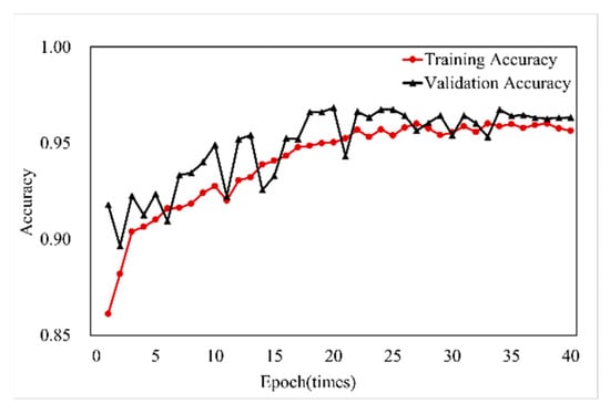
Figure 6.
The change curve of deep learning training and verification accuracy with the number of epochs based on the modified ResNet structure.
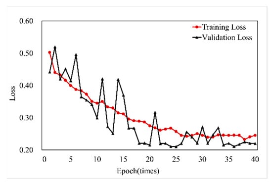
Figure 7.
The change curve of deep learning training and verification loss with the number of epochs based on the modified ResNet structure.
4.3. Visual Evaluation Results of ResNet-IST, VASTI, and NBR
To validate that the integration of features is superior to using SFs alone in detecting vegetation anomalies, we calculated and mapped the anomalous vegetation classifications for ten study areas via the ResNet-IST model, VASTI, and NBR. Figure 8I,II present false-color images (Band 5, Band 4, and Band 3) of the ten study areas before and after the fire. In this band combination, the colors of the ground features are intuitive, with red for vegetation—the healthier the vegetation is, the brighter the red. Figure 8III–V display the anomalous vegetation extraction results of the ResNet-IST model, VASTI, and NBR, respectively. In these images, black areas represent healthy vegetation unaffected by fire, whereas red areas indicate postfire anomalies.
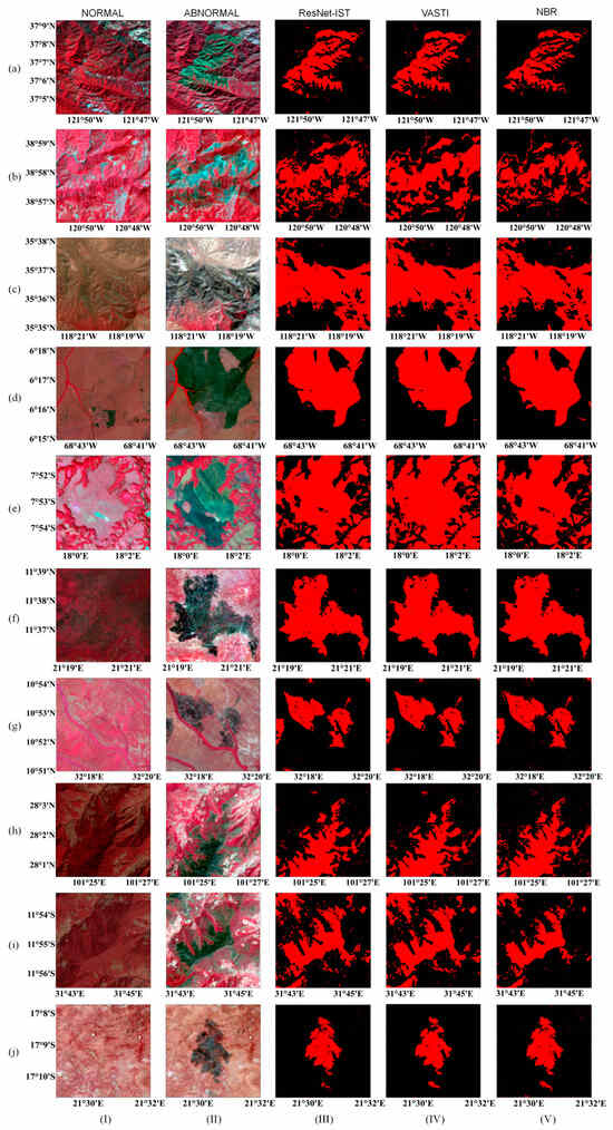
Figure 8.
Mapping of the study areas in normal and abnormal situations visual results of VASTI, ResNet-IST, and NBR. (a–j) represent the labels of the ten study sites. Column (I) shows the false-color remote sensing images of the validation areas before the fire, while Column (II) presents the false-color images after the fire. Columns (III), (IV), and (V) display the burned area extraction results obtained by the ResNet-IST model, the VASTI index, and the NBR index, respectively.
A comparison between Figure 8II,III reveals that the detection results from the ResNet-IST model largely align with the fire-affected vegetation areas, demonstrating its ability to handle this anomaly detection task effectively. Additionally, the results of ResNet-IST show a high degree of consistency with those of VASTI. However, in study areas (b), (e), and (j), the abnormal vegetation detected by ResNet-IST is significantly more precise than that identified by VASTI. In this study, although both the ResNet-IST framework and VASTI merge SFs and TFs, the methods of feature fusion differ significantly between the two approaches. Although the ResNet-IST model performs an implicit fusion of spectral and texture information without a predefined mathematical formula, deep learning is renowned for its superior computational capabilities. In contrast, VASTI emphasizes explicit fusion of different feature types, creating a new index model by combining features that show high differentiation between pre- and postfire vegetation via a specific mathematical formula. As a purely physical model, its information extraction capabilities are somewhat limited. NBR is one of the most commonly used indices for identifying fire-affected vegetation; it is based only on the spectral changes before and after a fire. Compared with the two comprehensive models, in certain study areas, such as region (a) and region (i), NBR extracts significantly smaller anomalous areas. This discrepancy may be due to the influence of shadows in complex terrains, where the spectral index alone causes spectral confusion at the edges, leading to misclassification. Additionally, in the study area (b), NBR mistakenly classifies the river as an anomalous vegetation area, likely because the reflectance changes or similarities between various land cover types cause NBR to erroneously categorize nonvegetative surfaces as anomalous vegetation.
4.4. Validation and Comparison of ResNet-IST, VASTI, and NBR
Owing to the limitations of visual interpretation for accuracy comparison, this study calculates three different accuracy metrics—UA, PA, and the kappa coefficient—for the ten study areas. Figure 9 compares these metrics across the three anomaly detection models. In summary, the ResNet-IST yielded superior performance among the other methods, as evidenced by the highest accuracy. The UA of the ResNet-IST classification results consistently remain at approximately 0.9, peaking at 0.96; the PA is near 0.92, with a maximum of 0.97; and the kappa coefficient ranges from a minimum of 0.76 to approximately 0.9 in most cases, reaching a peak of 0.95. These values are significantly superior to those of the other models. A comparison between the ResNet-IST model and VASTI shows a slight improvement of approximately 0.5% in UA for study areas (e), (f), and (g), whereas the other regions exhibit increases ranging from 1.1% to 3.8%. In terms of the PA, apart from study area (b), which only improved by 0.46%, the other regions exhibited a 1% to 4% enhancement. The improvement in the kappa coefficient is more noticeable, with the primary study areas demonstrating an accuracy increase of 2% to 8%. However, in areas (d), (f), and (g), the improvement was minimal. The difference between the ResNet-IST model and NBR is even more pronounced, particularly in study areas (a), (b), (h), (i), and (j). Compared with NBR, the ResNet-IST model improved the UA and kappa coefficients for fire-affected abnormal vegetation extraction by 10–20%, whereas the increase in PA, although slightly lower than the other two metrics, remained stable at approximately 5–10%. The results indicate that DL techniques offer a marked improvement in identifying burned vegetation, delivering superior performance compared with conventional physical models.
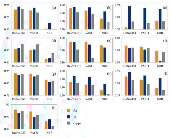
Figure 9.
Statistical maps of the UA, PA, and kappa coefficient of the three models for extracting vegetation anomaly regions. (a–j) illustrate the extraction accuracy maps of burned anomaly areas in the ten validation regions obtained using the ResNet-IST, VASTI, and NBR models, respectively.
When comparing the results of VASTI and NBR, apart from study areas (c), (e), and (f), VASTI’s UA is generally 6–10% higher than that of NBR. The improvement in PA fluctuated more, with most study areas showing an increase of 5–10%, whereas a few areas presented an improvement of approximately 2%. The increase in the kappa coefficient is also notable, with most regions exhibiting an approximate 10% increase. Notably, in study area (a), both the VASTI and ResNet-IST models achieved significant improvements in all three evaluation metrics compared with NBR, with the lowest increase reaching 37.4% and the highest at 58.3%. The data indicate that over half of the study areas demonstrated substantial improvements in accuracy. This finding demonstrates that the integration of texture and spectral features significantly enhances the accuracy of anomaly detection.
5. Discussion
5.1. Impact of Different Kinds of Input Features on ResNet-IST
To elucidate the impact of different input features on ResNet-IST, we employed SHAP values to quantify the contribution of each feature to the model. Figure 10 presents a visual analysis of the SHAP values for each feature, where SFs are represented in green, TFs in blue, and the integrated feature VASTI in yellow.
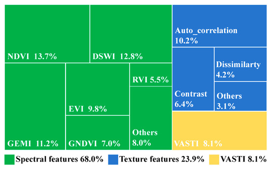
Figure 10.
Feature contribution analysis of inputs in ResNet-IST, categorized into three groups: spectral features, texture features, and comprehensive features.
The results indicate that SFs dominate the model, collectively accounting for 68.0% of the total contribution. Among them, NDVI, DSWI, and GEMI exhibit the highest contributions, consistent with their widespread application in assessing vegetation health, making them particularly responsive to burned vegetation. The nine TFs contribute 23.9% to the model, serving as auxiliary information. Among these, autocorrelation ranked first, followed by contrast and dissimilarity. The remaining six TFs make relatively minor contributions, collectively accounting for only 3.1%. Notably, the integrated VASTI contributes only 8.1% to the model, lower than certain individual spectral and texture features. This lower contribution may be attributed to feature redundancy, as VASTI inherently incorporates multiple VIs and TFs. Otherwise, composite features involve multiple component parameters, which may lead to gradient direction conflicts during backpropagation. This can result in unstable weight updates within the model, ultimately causing the contribution of composite features to be significantly weaker than that of individual dominant features [78]. However, this explanation remains tentative and would require further experimental validation before being confirmed.
Overall, although SFs remain the dominant contributors due to the intrinsic characteristics of the target being identified, TFs provide a certain degree of improvement to the model. When vegetation suffers disasters, spectral differences are significantly more pronounced than texture variations, which explains their higher contribution to the model. However, SHAP contribution values only reflect the influence of features in the current model but do not directly measure their classification accuracy or predictive capability [79]. Therefore, a high SHAP value indicates that the feature has a significant influence on the model’s decision-making but does not imply that the feature itself can independently achieve accurate classification or prediction.
5.2. Capability of the ResNet-IST Framework for Detecting Fire-Affected Vegetation
The visual evaluations of vegetation anomaly detection for the ten study areas demonstrated that the ResNet-IST model can reliably classify the fire-affected areas at a 30 m spatial resolution (Figure 8). Moreover, the accuracy of burned area detection when the ResNet-IST framework is used is significantly better than that when single-physical indices (VASTI and NBR) are used (Figure 9), with a UA of approximately 0.93 in most regions. The PA remained stable at 0.92, peaking at 0.97. The kappa coefficient fluctuated around 0.9, reaching as high as 0.95. However, the ResNet-IST algorithm exhibited significant terrain variability, performing well in study areas (a), (c), (h), (i), and (j), with accuracies notably higher than those of VASTI. In contrast, the accuracy improvements in study areas (d), (f), and (g) were minimal. Figure 8i shows that the terrain in these areas is relatively flat compared with that in other areas, where simple physical models are sufficient for anomaly detection. Previous research on ResNet architectures for image recognition has shown that ResNets often outperform more complex networks because of their strong generalization performance, allowing them to extract more detailed feature information in complex terrains such as those in areas (a) and (c) [80]. The shortcut connections between layers significantly reduce the training time and computational resources. In addition to the enhancements and optimizations provided by the architecture itself, the inclusion of DL algorithms also benefits the feature fusion process [81]. Thus, the ResNet-IST algorithm for merging various spectral and textural features improves the detection of burned vegetation.
Our study revealed that the use of the ResNet-IST model for abnormal forest detection not only provides superior results to those of VASTI but also performs better than the single spectral index (NBR). The outcomes from the ResNet-IST models were significantly greater than those of NBR, with a general accuracy improvement of 10%, which demonstrates that the ResNet-IST model notably improves performance in abnormal vegetation extraction, both in terms of computational principles and feature fusion capabilities [82]. For NBR, its ability to detect burned vegetation relies solely on abrupt changes in the NIR and SWIR bands during vegetation anomalies. Although spectral changes provide a direct indication of vegetation status, they inevitably lead to spectral confusion at the boundaries of burned areas [83]. While VASTI addresses this issue by incorporating spatial texture information, the computational power of its physical model remains limited. The skip connections in ResNet effectively address the issues of vanishing and exploding gradients in deep networks. This allows ResNet to extract more comprehensive image features while reducing training time and maximizing the utilization of information within the imagery [28]. Therefore, the ResNet-IST framework makes the best use of the spectral and spatial information of the sample inputs in the process of merging the SFs and TFs.
5.3. The Uncertainties of the ResNet-IST Model
While the ResNet-IST model demonstrates certain advantages in anomalous vegetation extraction, it should be emphasized that some uncertainties remain owing to the nontransparent nature of network iterations. First, the data quality and variability may influence the capability of the model. The precision of a model is significantly influenced by the quality of the input data [84]. Variations in samples caused by atmospheric fluctuations, seasonal shifts, and lighting differences may lead to inconsistencies. These discrepancies can contribute to uncertainties in the predictions of the model. Although we preprocessed the images before constructing the dataset to minimize the adverse impact of the images on the model, some imperfect samples were still inevitable. Second, different feature combinations lead to different results. While integrating SFs and TFs is highly excellent for anomaly detection, achieving optimal fusion of these features remains challenging [85]. Uncertainties may arise in how effectively the model weights each feature, as the significance of spectral information can vary with vegetation type and environmental conditions [86]. Additionally, when burned areas are obscured by unburned forest canopies, spectral confusion may arise at the boundaries of these anomalous regions, so VIs may provide false information. Therefore, determining the dominant role of SFs and TFs in combination is critical. Third, the parameter settings of the GLCM can influence the extracted TFs, and different combinations may introduce uncertainty. GLCM is defined by four main parameters: direction, step size, window size, and gray levels. Variations in these parameters affect the numerical values and spatial patterns of TFs. For example, step size and window size control the spatial scale captured, while direction and gray levels affect feature sensitivity and detail representation. Since any permutation of these parameters can produce numerous outcomes, GLCM-derived features inherently carry a degree of uncertainty, which may impact model stability and transferability across regions or datasets.
The characteristics of the ResNet-IST model also introduce a certain degree of uncertainty. The DL models are frequently described as “black boxes” because it is difficult to trace how specific inputs (such as spectral and texture features) are transformed into outputs (such as predictions of abnormal vegetation) [87]. Therefore, interpreting the decision-making process involving complex layers of mathematical operations is challenging. The lack of interpretability introduces significant uncertainty in understanding the model’s reliability, especially in critical applications such as environmental monitoring or disaster response [88]. For example, if ResNet were to predict the presence of burned vegetation, it may be unclear which features contributed the most to the decision. This uncertainty can undermine trust in the model’s predictions and make it harder to identify errors or biases. Without interpretability, it becomes difficult to explain why a model fails or succeeds in certain cases, limiting its practical application and reducing the ability to improve or troubleshoot the model effectively [89].
5.4. Merits and Limitations of the ResNet-IST Model
The experimental results indicate that the ResNet-IST model employed in this study outperforms the explicit texture-spectral composite feature model, VASTI, developed in previous research. The primary advantages of the ResNet-IST model can be summarized as follows: First, the incorporation of a deep residual learning network enhances the robustness of the final classification. Through iterative training, the model converges to a relatively stable outcome, with each iteration providing feedback for subsequent iterations, progressively optimizing performance to achieve the best results of the model [41]. Compared with other DL algorithms, ResNet is more robust to variations in data distribution and model parameters [90]. Second, the algorithmic model used in this study requires less computational power. The deep residual network demands fewer computational resources than do other models [91]. For example, although the VGG network is much shallower than that of ResNet, both have a similar number of parameters. This is because ResNet eliminates the need for fully connected layers and utilizes a bottleneck structure. It should also be noted that ResNet-IST is built upon the ResNet50 backbone, but extends it by incorporating both spectral and texture features in an implicit manner. While ResNet50 alone primarily captures spectral information, ResNet-IST integrates complementary texture features, enabling it to achieve higher anomaly detection accuracy. This design allows ResNet-IST to outperform the baseline ResNet50 in terms of robustness and generalization.
Although the ResNet-IST model has significant advantages in identifying anomalous vegetation areas, some limitations should be noted. First, there is a higher memory requirement during the computational process. Deep residual networks are generally more memory efficient during inference; however, their memory usage increases significantly during the training process [92]. Second, the generalizability of the model has not been validated. Although the model may perform well on training and validation datasets, there is uncertainty in its ability to generalize to unseen data [93]. Differences in vegetation types, environmental conditions, and geographic regions not represented in the training data could impact the robustness and accuracy of the model. Third, the selection of dataset samples introduces certain limitations to the experimental results of this study. Although ten research sites were selected from around the world, these sites represent only six types of vegetation cover, leaving many other types unconsidered. Additionally, this study did not account for the influences of topography and terrain, nor was classification validation conducted under varying conditions. Therefore, dataset selection imposes some limitations on the model. It is important to note that these limitations extend beyond vegetation types and topographic factors to the representativeness of the fire events themselves. While the ten sites were chosen based on physical separation, habitat diversity, the availability of high-quality Landsat-8 imagery, and clear fire boundaries, there is a substantial imbalance in sample sizes across sites (e.g., 29 samples in site (h) versus 267 in site (j)), which may affect the robustness and generalizability of the model. Consequently, the current results primarily reflect the conditions of the selected sites and fire events, rather than being broadly generalizable to all fire types and ecosystems. Nevertheless, these sites provide a standardized dataset that enables the comparative evaluation of different feature extraction methods and the assessment of the ResNet-IST model’s performance. Future work will aim to expand the dataset to include additional fire events independent of the training set, encompassing a wider range of vegetation types, fire intensities, and environmental conditions, thereby improving statistical rigor, model generalizability, and robustness across diverse scenarios.
Furthermore, the applicability of the ResNet-IST model in broader contexts requires careful consideration. While the model shows promising results on Landsat-8 imagery, its performance on other satellite sensors, such as Sentinel-2, MODIS, or SAR platforms, may vary due to differences in spectral resolution, revisit time, and radiometric characteristics. Environmental heterogeneity, including variations in climate, soil type, and vegetation structure, could also influence model performance, potentially reducing accuracy in ecosystems not represented in the current training dataset. In near-real-time monitoring scenarios, computational costs, data latency, and preprocessing requirements must be addressed to ensure timely anomaly detection. Therefore, while the ResNet-IST model is robust within the scope of this study, careful calibration and validation are necessary before applying it to other sensors, regions, or operational settings. These considerations highlight both the potential and the current limitations of the model for general-purpose fire-affected vegetation detection. In future research, we aim to consider a wider range of factors to improve the robustness and generalizability of the model.
6. Conclusions
Forest fires reduce the ecosystem services and biodiversity of vegetation. Accurate extraction of burned areas is crucial for post-disaster assessment and restoration efforts. Although existing fire indices can effectively identify anomalous vegetation areas, they still have certain limitations. Our new method, ResNet-IST, represents a significant advancement in detecting anomalous vegetation areas. This method leverages the DL capabilities of ResNet50 to capture complex spatial and spectral variations, enabling more precise identification of burned or damaged vegetation. This approach allows for an implicit, adaptive combination of features, enhancing detection accuracy and reducing sensitivity to environmental variations such as lighting or seasonal changes. The main findings and contributions of this study are summarized as follows:
- (1)
- We developed a potential vegetation anomaly detection model named the ResNet-IST by merging spectral and texture features using a DL algorithm based on the ResNet50 architecture. Unlike traditional mathematical models, the performance of ResNet-IST significantly increases the computational capacity, and the iterative nature of the model improves its robustness.
- (2)
- In most study areas, the ResNet-IST model showed significant improvement in validation, with accuracies that were mostly 3% higher than those of VASTI and 5–15% higher than those of NBR. The results demonstrate its superior performance in anomaly detection tasks. Additionally, the recognition accuracy of VASTI is notably superior to that of NBR, indicating that incorporating TFs compensates for the limitations of SFs.
In conclusion, the ResNet-IST model developed in this study has proven its ability to accurately detect fire-induced anomalous vegetation areas on a global scale, offering new methods and insights for the extraction and analysis of burned areas worldwide. Nevertheless, this study also has limitations. For instance, the model has only been tested on a limited number of sites and has not yet been systematically validated across different fire intensities, vegetation types, or ecological regions. Future research should aim to expand the evaluation to broader contexts, including the application of the model to Sentinel-2 data with higher spatial resolution, integration with SAR sensors to enhance performance under cloudy or smoke-covered conditions, and testing in tropical biomes where vegetation complexity and fire dynamics differ significantly from the current study sites. These directions will help further improve the robustness, generalizability, and practical applicability of the proposed model.
Author Contributions
Conceptualization, J.F. and Y.Y.; methodology, J.F., Y.Y. and J.C.; software, J.F. and Z.X.; validation, B.J. and F.Q.; formal analysis, J.F.; investigation, L.L. and L.Z.; data curation, J.B.F. Fisher; writing—original draft preparation, J.F.; writing—review and editing, Y.Y. and J.C.; visualization, Y.L. and X.Z. (Xueyi Zhang); supervision, X.Z. (Xiaotong Zhang); funding acquisition, Y.Y. All authors have read and agreed to the published version of the manuscript.
Funding
This work was supported by the Natural Science Fund of China (No. 42192581, No. 42192580 and No. 42171310).
Data Availability Statement
The data presented in this study are available at https://doi.org/10.3334/ORNLDAAC/1642 (accessed on 5 September 2022) and https://earthexplorer.usgs.gov/ (accessed on 18 July 2023).
Acknowledgments
We gratefully acknowledge the National Aeronautics and Space Administration (NASA) for providing the Global Fire Atlas [48]. The Landsat 8 imagery used in this study was obtained from the United States Geological Survey (USGS) EarthExplorer platform (https://earthexplorer.usgs.gov/).
Conflicts of Interest
The authors declare no conflicts of interest.
References
- Flannigan, M.D.; Amiro, B.D.; Logan, K.A.; Stocks, B.J.; Wotton, B.M. Forest Fires and Climate Change in the 21ST Century. Mitig. Adapt. Strateg. Glob. Chang. 2006, 11, 847–859. [Google Scholar] [CrossRef]
- Pew, K.L.; Larsen, C.P.S. GIS analysis of spatial and temporal patterns of human-caused wildfires in the temperate rain forest of Vancouver Island, Canada. For. Ecol. Manag. 2001, 140, 1–18. [Google Scholar] [CrossRef]
- Carmenta, R.; Parry, L.; Blackburn, A.; Vermeylen, S.; Barlow, J. Understanding Human-Fire Interactions in Tropical Forest Regions: A Case for Interdisciplinary Research across the Natural and Social Sciences. Ecol. Soc. 2011, 16, 22. [Google Scholar] [CrossRef]
- Tanase, M.A.; Kennedy, R.; Aponte, C. Fire severity estimation from space: A comparison of active and passive sensors and their synergy for different forest types. Int. J. Wildland Fire 2015, 24, 1062–1075. [Google Scholar] [CrossRef]
- Vhengani, L.; Frost, P.; Lai, C.; Booi, N.; Dool, R.v.D.; Raath, W. Multitemporal burnt area mapping using Landsat 8: Merging multiple burnt area indices to highlight burnt areas. In Proceedings of the IEEE International Geoscience and Remote Sensing Symposium (IGARSS), Milan, Italy, 26–31 July 2015; IEEE: New York, NY, USA, 2015. [Google Scholar]
- Brewer, C.K.; Winne, J.C.; Redmond, R.L.; Opitz, D.W. Classifying and mapping wildfire severity: A comparison of methods. Photogramm. Eng. Remote Sens. 2005, 71, 1311–1320. [Google Scholar] [CrossRef]
- Poulos, H.M.; Barton, A.M.; Koch, G.W.; Kolb, T.E.; Thode, A.E. Wildfire severity and vegetation recovery drive post-fire evapotranspiration in a southwestern pine-oak forest, Arizona, USA. Remote Sens. Ecol. Conserv. 2021, 7, 579–591. [Google Scholar] [CrossRef]
- Chuvieco, E.; Congalton, R.G. Mapping and inventory of forest fires from digital processing of tm data. Geocarto Int. 1988, 3, 41–53. [Google Scholar] [CrossRef]
- Pascolini-Campbell, M.; Lee, C.; Stavros, N.; Fisher, J.B. ECOSTRESS reveals pre-fire vegetation controls on burn severity for Southern California wildfires of 2020. Glob. Ecol. Biogeogr. 2022, 31, 1976–1989. [Google Scholar] [CrossRef]
- Joshi, R.C.; Jensen, A.; Pascolini-Campbell, M.; Fisher, J.B. Coupling between evapotranspiration, water use efficiency, and evaporative stress index strengthens after wildfires in New Mexico, USA. Int. J. Appl. Earth Obs. 2024, 135, 12. [Google Scholar] [CrossRef]
- Veraverbeke, S.; Gitas, I.; Katagis, T.; Polychronaki, A.; Somers, B.; Goossens, R. Assessing post-fire vegetation recovery using red-near infrared vegetation indices: Accounting for background and vegetation variability. ISPRS J. Photogramm. Remote Sens. 2012, 68, 28–39. [Google Scholar] [CrossRef]
- Tucker, C.J. Red and Photographic Infrared Linear Combinations for Monitoring Vegetation. Remote Sens. Environ. 1979, 8, 127–150. [Google Scholar] [CrossRef]
- Lhermitte, S.; Verbesselt, J.; Verstraeten, W.W.; Veraverbeke, S.; Coppin, P. Assessing intra-annual vegetation regrowth after fire using the pixel based regeneration index. ISPRS J. Photogramm. Remote Sens. 2011, 66, 17–27. [Google Scholar] [CrossRef]
- Fernández-García, V.; Kull, C.A. Refining historical burned area data from satellite observations. Int. J. Appl. Earth Obs. Geoinf. 2023, 120, 12. [Google Scholar] [CrossRef]
- Pinty, B.; Verstraete, M.M. GEMI—A nonlinear index to monitor global vegetation from satellites. Vegetatio 1992, 101, 15–20. [Google Scholar] [CrossRef]
- Grigorov, B. GEMI—A Possible Tool for Identification of Disturbances in Confirerous Forests in Pernik Povince (Western Bulgaria). Civ. Environ. Eng. Rep. 2022, 32, 116–122. [Google Scholar] [CrossRef]
- Meena, S.V.; Dhaka, V.S.; Sinwar, D. Exploring the Role of Vegetation Indices in Plant Diseases Identification. In Proceedings of the 2020 Sixth International Conference on Parallel, Distributed and Grid Computing (PDGC), Waknaghat, India, 6–8 November 2020. [Google Scholar]
- García, M.J.L.; Caselles, V. Mapping burns and natural reforestation using thematic Mapper data. Geocarto Int. 1991, 6, 31–37. [Google Scholar] [CrossRef]
- Gerard, F.; Plummer, S.; Wadsworth, R.; Sanfeliu, A.F.; Iliffe, L.; Balzter, H.; Wyatt, B. Forest fire scar detection in the boreal forest with multitemporal SPOT-VEGETATION data. IEEE Trans. Geosci. Remote Sens. 2003, 41, 2575–2585. [Google Scholar] [CrossRef]
- Chuvieco, E.; Martín, M.P. Cartografía de Grandes Incendios Forestales en la Península Ibérica a Partir de Imágenes NOAA-AVHRR; Universidad de Alcalá de Henares: Alcalá de Henares, Spain, 1998. [Google Scholar]
- Majdar, R.S.; Ghassemian, H. A probabilistic SVM approach for hyperspectral image classification using spectral and texture features. Int. J. Remote Sens. 2017, 38, 4265–4284. [Google Scholar] [CrossRef]
- Li, C.; Liu, Q.; Li, B.R.; Liu, L. Investigation of Recognition and Classification of Forest Fires Based on Fusion Color and Textural Features of Images. Forests 2022, 13, 19. [Google Scholar] [CrossRef]
- Mitri, G.H.; Gitas, I.Z. A semi-automated object-oriented model for burned area mapping in the Mediterranean region using Landsat-TM imagery. Int. J. Wildland Fire 2004, 13, 367–376. [Google Scholar] [CrossRef]
- Shama, A.; Zhang, R.; Zhan, R.Q.; Wang, T.; Xie, L.; Bao, X.; Lv, J. A Burned Area Extracting Method Using Polarization and Texture Feature of Sentinel-1A Images. IEEE Geosci. Remote Sens. Lett. 2023, 20, 5. [Google Scholar] [CrossRef]
- Fan, J.H.; Yao, Y.J.; Tang, Q.X.; Zhang, X.; Xu, J.; Yu, R.; Liu, L.; Xie, Z.; Ning, J.; Zhang, L. A Hybrid Index for Monitoring Burned Vegetation by Combining Image Texture Features with Vegetation Indices. Remote Sens. 2024, 16, 1539. [Google Scholar] [CrossRef]
- Krizhevsky, A.; Sutskever, I.; Hinton, G.E. ImageNet Classification with Deep Convolutional Neural Networks. Commun. Acm 2017, 60, 84–90. [Google Scholar] [CrossRef]
- Szegedy, C.; Liu, W.; Jia, Y.Q.; Sermanet, P.; Reed, S.; Anguelov, D.; Erhan, D.; Vanhoucke, V.; Rabinovich, A.; Liu, W.; et al. Going Deeper with Convolutions. In Proceedings of the IEEE Conference on Computer Vision and Pattern Recognition (CVPR), Boston, MA, USA, 7–12 June 2015; IEEE: New York, NY, USA, 2015. [Google Scholar]
- He, K.M.; Zhang, X.Y.; Ren, S.Q.; Sun, J. Identity Mappings in Deep Residual Networks. In Proceedings of the 14th European Conference on Computer Vision (ECCV), Amsterdam, The Netherlands, 8–16 October 2016; Springer International Publishing: Cham, Switzerland, 2016. [Google Scholar]
- Chen, L.C.; Papandreou, G.; Kokkinos, I.; Murphy, K.; Yuille, A.L. DeepLab: Semantic Image Segmentation with Deep Convolutional Nets, Atrous Convolution, and Fully Connected CRFs. IEEE Trans. Pattern Anal. Mach. Intell. 2018, 40, 834–848. [Google Scholar] [CrossRef] [PubMed]
- Lin, G.S.; Milan, A.; Shen, C.H.; Reid, I. RefineNet: Multi-Path Refinement Networks for High-Resolution Semantic Segmentation. In Proceedings of the 30th IEEE/CVF Conference on Computer Vision and Pattern Recognition (CVPR), Honolulu, HI, USA, 21–26 July 2017; IEEE: New York, NY, USA, 2017. [Google Scholar]
- Zhao, H.S.; Shi, J.P.; Qi, X.J.; Wang, X.; Jia, J. Pyramid Scene Parsing Network. In Proceedings of the 30th IEEE/CVF Conference on Computer Vision and Pattern Recognition (CVPR), Honolulu, HI, USA, 21–26 July 2017; IEEE: New York, NY, USA, 2017. [Google Scholar]
- He, K.M.; Zhang, X.Y.; Ren, S.Q.; Sun, J. Spatial Pyramid Pooling in Deep Convolutional Networks for Visual Recognition. IEEE Trans. Pattern Anal. Mach. Intell. 2015, 37, 1904–1916. [Google Scholar] [CrossRef] [PubMed]
- Ren, S.Q.; He, K.M.; Girshick, R.; Sun, J. Faster R-CNN: Towards Real-Time Object Detection with Region Proposal Networks. IEEE Trans. Pattern Anal. Mach. Intell. 2017, 39, 1137–1149. [Google Scholar] [CrossRef]
- Hornik, K.; Stinchcombe, M.; White, H. Multilayer feedforward networks are universal approximators. Neural Netw. 1989, 2, 359–366. [Google Scholar] [CrossRef]
- Lecun, Y.; Bottou, L.; Bengio, Y.; Haffner, P. Gradient-based learning applied to document recognition. Proc. IEEE 1998, 86, 2278–2324. [Google Scholar] [CrossRef]
- Zeiler, M.D.; Krishnan, D.; Taylor, G.W.; Fergus, R. Deconvolutional Networks. In Proceedings of the 23rd IEEE Conference on Computer Vision and Pattern Recognition (CVPR), San Francisco, CA, USA, 13–18 June 2010; IEEE Computer Society: Los Alamitos, CA, USA, 2010. [Google Scholar]
- Yu, K.; Lin, Y.Q.; Lafferty, J. Learning Image Representations from the Pixel Level via Hierarchical Sparse Coding. In Proceedings of the IEEE Conference on Computer Vision and Pattern Recognition (CVPR), Colorado Springs, CO, USA, 20–25 June 2011; IEEE: New York, NY, USA, 2011. [Google Scholar]
- Salakhutdinov, R.; Hinton, G. Deep Boltzmann Machines. In Proceedings of the Twelfth International Conference on Artificial Intelligence and Statistics, Clearwater Beach, FL, USA, 16–18 April 2009; pp. 448–455. [Google Scholar]
- Vincent, P.; Larochelle, H.; Bengio, Y.; Manzagol, P.-A. Extracting and Composing Robust Features with Denoising Autoencoders; proceedings of the Machine Learning. In Proceedings of the Twenty-Fifth International Conference (ICML 2008), Helsinki, FL, USA, 5–9 June 2008. [Google Scholar]
- He, K.M.; Zhang, X.Y.; Ren, S.Q.; Sun, J. Deep Residual Learning for Image Recognition. In Proceedings of the 2016 IEEE Conference on Computer Vision and Pattern Recognition (CVPR), Las Vegas, NV, USA, 27–30 June 2016. [Google Scholar]
- Li, H.; Hu, B.X.; Li, Q.; Jing, L. CNN-Based Individual Tree Species Classification Using High-Resolution Satellite Imagery and Airborne LiDAR Data. Forests 2021, 12, 1697. [Google Scholar] [CrossRef]
- Wang, M.; Zhang, X.; Niu, X.; Wang, F.; Zhang, X. Scene Classification of High-Resolution Remotely Sensed Image Based on ResNet. J. Geovisualization Spat. Anal. 2019, 3, 16. [Google Scholar] [CrossRef]
- Park, M.; Tran, D.Q.; Lee, S.; Wang, F.; Zhang, X. Multilabel Image Classification with Deep Transfer Learning for Decision Support on Wildfire Response. Remote Sens. 2021, 13, 3985. [Google Scholar] [CrossRef]
- Zhang, L.; Wang, M.Y.; Fu, Y.J.; Ding, Y. A Forest Fire Recognition Method Using UAV Images Based on Transfer Learning. Forests 2022, 13, 975. [Google Scholar] [CrossRef]
- Dogan, S.; Barua, P.D.; Kutlu, H.; Baygin, M.; Fujita, H.; Tuncer, T.; Acharya, U. Automated accurate fire detection system using ensemble pretrained residual network. Expert Syst. Appl. 2022, 203, 9. [Google Scholar] [CrossRef]
- Tsalera, E.; Papadakis, A.; Voyiatzis, I.; Samarakou, M. CNN-based, contextualized, real-time fire detection in computational resource-constrained environments. Energy Rep. 2023, 9, 247–257. [Google Scholar] [CrossRef]
- Hu, X.K.; Zhang, P.Z.; Ban, Y.F.; Rahnemoonfar, M. GAN-based SAR and optical image translation for wildfire impact assessment using multi-source remote sensing data. Remote Sens. Environ. 2023, 289, 13. [Google Scholar] [CrossRef]
- Andela, N.; Morton, D.C.; Giglio, L.; Paugam, R.; Chen, Y.; Hantson, S.; van der Werf, G.R. Global Fire Atlas with Characteristics of Individual Fires Size, Duration, Speed and Direction. Earth Syst. Sci. Data 2019, 11, 529–552. [Google Scholar] [CrossRef]
- Irons, J.R.; Dwyer, J.L.; Barsi, J.A. The next Landsat satellite: The Landsat Data Continuity Mission. Remote Sens. Environ. 2012, 122, 11–21. [Google Scholar] [CrossRef]
- Simonyan, K.; Zisserman, A. Very Deep Convolutional Networks for Large-Scale Image Recognition. arXiv 2014, arXiv:1409.1556. [Google Scholar]
- Moghadam, P.; Ward, D.; Goan, E.; Jayawardena, S.; Sikka, P.; Hernandez, E. Plant Disease Detection using Hyperspectral Imaging. In Proceedings of the International Conference on Digital Image Computing—Techniques and Applications (DICTA), Sydney, Australia, 29 November–1 December 2017; IEEE: New York, NY, USA, 2017. [Google Scholar]
- Wu, G.S.; Fang, Y.L.; Jiang, Q.Y.; Cui, M.; Li, N.; Ou, Y.; Diao, Z.; Zhang, B. Early identification of strawberry leaves disease utilizing hyperspectral imaging combing with spectral features, multiple vegetation indices and textural features. Comput. Electron. Agric. 2023, 204, 12. [Google Scholar] [CrossRef]
- Carlson, T.N.; Ripley, D.A. On the relation between NDVI, fractional vegetation cover, and leaf area index. Remote Sens. Environ. 1997, 62, 241–252. [Google Scholar] [CrossRef]
- Liu, H.Q.; Huete, A. A feedback based modification of the ndvi to minimize canopy background and atmospheric noise. IEEE Trans. Geosci. Remote Sens. 1995, 33, 457–465. [Google Scholar] [CrossRef]
- Pearson, R.L.; Miller, L.D. Remote Mapping of Standing Crop Biomass for Estimation of Productivity of the Shortgrass Prairie. Remote Sens. Environ. VIII 1972, 2, 1357–1381. [Google Scholar] [CrossRef]
- Gitelson, A.A.; Kaufman, Y.J.; Merzlyak, M.N. Use of a green channel in remote sensing of global vegetation from EOS-MODIS. Remote Sens. Environ. 1996, 58, 289–298. [Google Scholar] [CrossRef]
- Broge, N.H.; Leblanc, E. Comparing prediction power and stability of broadband and hyperspectral vegetation indices for estimation of green leaf area index and canopy chlorophyll density. Remote Sens. Environ. 2001, 76, 156–172. [Google Scholar] [CrossRef]
- Jordan, C.F. Derivation of leaf-area index from quality of light on forest floor. Ecology 1969, 50, 663–666. [Google Scholar] [CrossRef]
- Galvao, L.S.; Formaggio, A.R.; Tisot, D.A. Discrimination of sugarcane varieties in southeastern brazil with EO-1 hyperion data. Remote Sens. Environ. 2005, 94, 523–534. [Google Scholar] [CrossRef]
- Qi, J.; Chehbouni, A.; Huete, A.R.; Kerr, Y.H.; Sorooshian, S. A modified soil adjusted vegetation index. Remote Sens. Environ. 1994, 48, 119–126. [Google Scholar] [CrossRef]
- Gitelson, A.A.; Viña, A.; Arkebauer, T.J.; Rundquist, D.C.; Keydan, G.; Leavitt, B. Remote estimation of leaf area index and green leaf biomass in maize canopies. Geophys. Res. Lett. 2003, 30, 4. [Google Scholar] [CrossRef]
- Pu, R.L.; Gong, P.; Yu, Q. Comparative analysis of EO-1 ALI and Hyperion, and Landsat ETM+ data for mapping forest crown closure and leaf area index. Sensors 2008, 8, 3744–3766. [Google Scholar] [CrossRef] [PubMed]
- Rao, N.R.; Garg, P.K.; Ghosh, S.K.; Dadhwal, V.K. Estimation of leaf total chlorophyll and nitrogen concentrations using hyperspectral satellite imagery. J. Agric. Sci. 2008, 146, 65–75. [Google Scholar]
- Smith, J.R.; Chang, S.F. Automated binary texture feature sets for image retrieval. In Proceedings of the Acoustics, Speech, and Signal Processing, Atlanta, GA, USA, 9 May 1996. [Google Scholar]
- Baraldi, A.; Parmiggiani, F. An investigation of the textural characteristics associated with gray-level cooccurrence matrix statistical parameters. IEEE Trans. Geosci. Remote Sens. 1995, 33, 293–304. [Google Scholar] [CrossRef]
- Haralick, R.M.; Shanmugam, K.; Dinstein, I. Textural features for image classification. IEEE Trans. Syst. Man Cybern. 1973, SMC3, 610–621. [Google Scholar] [CrossRef]
- Conners, R.W.; Trivedi, M.M.; Harlow, C.A. Segmentation of a high-resolution urban scene using texture operators. Comput. Vis. Graph. Image Process. 1984, 25, 273–310. [Google Scholar] [CrossRef]
- Yuan, J.Y.; Wang, D.L.; Li, R.X. Remote Sensing Image Segmentation by Combining Spectral and Texture Features. IEEE Trans. Geosci. Remote Sens. 2014, 52, 16–24. [Google Scholar] [CrossRef]
- Zhou, Y.; Wang, Z.; Zheng, S.; Zhou, L.; Dai, L.; Luo, H.; Zhang, Z.; Sui, M. Optimization of automated garbage recognition model based on ResNet-50 and weakly supervised CNN for sustainable urban development. Alex. Eng. J. 2024, 108, 415–427. [Google Scholar] [CrossRef]
- Xie, S.N.; Girshick, R.; Dollár, P.; Tu, Z.; He, K. Aggregated Residual Transformations for Deep Neural Networks. In Proceedings of the 30th IEEE/CVF Conference on Computer Vision and Pattern Recognition (CVPR), Honolulu, HI, USA, 21–26 July 2017; IEEE: New York, NY, USA, 2017. [Google Scholar]
- Lu, Z.Y.; Lu, J.; Ge, Q.B.; Zhan, T. Multi-object Detection Method based on YOLO and ResNet Hybrid Networks. In Proceedings of the 4th IEEE International Conference on Advanced Robotics and Mechatronics (ICARM), Osaka, Japan, 3–5 July 2019; IEEE: New York, NY, USA, 2019. [Google Scholar]
- Pan, T.S.; Huang, H.C.; Lee, J.C.; Chen, C.H. Multi-scale ResNet for real-time underwater object detection. Signal Image Video Process. 2021, 15, 941–949. [Google Scholar] [CrossRef]
- Pohlen, T.; Hermans, A.; Mathias, M.; Leibe, B. Full-Resolution Residual Networks for Semantic Segmentation in Street Scenes. In Proceedings of the 30th IEEE/CVF Conference on Computer Vision and Pattern Recognition (CVPR), Honolulu, HI, USA, 21–26 July 2017; IEEE: New York, NY, USA, 2017. [Google Scholar]
- Xia, K.J.; Yin, H.S.; Zhang, Y.D. Deep Semantic Segmentation of Kidney and Space-Occupying Lesion Area Based on SCNN and ResNet Models Combined with SIFT-Flow Algorithm. J. Med. Syst. 2019, 43, 12. [Google Scholar] [CrossRef]
- Lipovetsky, S.; Conklin, M. Analysis of regression in game theory approach. Appl. Stoch. Models Bus. Ind. 2001, 17, 319–330. [Google Scholar] [CrossRef]
- Fujimoto, K.; Kojadinovic, I.; Marichal, J.-L. Axiomatic characterizations of probabilistic and cardinal-probabilistic interaction indices. Games Econ. Behav. 2006, 55, 72–99. [Google Scholar] [CrossRef]
- Lundberg, S.M.; Erion, G.G.; Lee, S.I. Consistent Individualized Feature Attribution for Tree Ensembles. arXiv 2018, arXiv:1802.03888. [Google Scholar]
- Tan, M.; Pang, R.; Le, Q.V. Efficientdet: Scalable and efficient object detection. In Proceedings of the IEEE/CVF Conference on Computer Vision and Pattern Recognition, Seattle, WA, USA, 13–19 June 2020. [Google Scholar]
- Doshi-Velez, F.; Kim, B. Towards A Rigorous Science of Interpretable Machine Learning. arXiv 2017, arXiv:1702.08608. [Google Scholar] [CrossRef]
- Fuentes, A.; Yoon, S.; Kim, S.C.; Park, D.S. A Robust Deep-Learning-Based Detector for Real-Time Tomato Plant Diseases and Pests Recognition. Sensors 2017, 17, 2022. [Google Scholar] [CrossRef] [PubMed]
- Roy, S.K.; Manna, S.; Song, T.C.; Bruzzone, L. Attention-Based Adaptive Spectral-Spatial Kernel ResNet for Hyperspectral Image Classification. IEEE Trans. Geosci. Remote Sens. 2021, 59, 7831–7843. [Google Scholar] [CrossRef]
- Gu, J.X.; Wang, Z.H.; Kuen, J.; Ma, L.; Shahroudy, A.; Shuai, B.; Liu, T.; Wang, X.; Wang, G.; Cai, J.; et al. Recent advances in convolutional neural networks. Pattern Recognit. 2018, 77, 354–377. [Google Scholar] [CrossRef]
- Balling, J.; Herold, M.; Reiche, J. How textural features can improve SAR-based tropical forest disturbance mapping. Int. J. Appl. Earth Obs. Geoinf. 2023, 124, 14. [Google Scholar] [CrossRef]
- Alzubaidi, L.; Zhang, J.L.; Humaidi, A.J.; Al-Dujaili, A.; Duan, Y.; Al-Shamma, O.; Santamaría, J.; Fadhel, M.A.; Al-Amidie, M.; Farhan, L. Review of deep learning: Concepts, CNN architectures, challenges, applications, future directions. J. Big Data 2021, 8, 74. [Google Scholar] [CrossRef]
- Hu, X.Y.; Tao, C.V.; Prenzel, B. Automatic segmentation of high-resolution satellite imagery by integrating texture, intensity, and color features. Photogramm. Eng. Remote Sens. 2005, 71, 1399–1406. [Google Scholar] [CrossRef]
- Ghasemi, N.; Sahebi, M.R.; Mohammadzadeh, A. Biomass Estimation of a Temperate Deciduous Forest Using Wavelet Analysis. IEEE Trans. Geosci. Remote Sens. 2013, 51, 765–776. [Google Scholar] [CrossRef]
- Shafiq, M.; Gu, Z.Q. Deep Residual Learning for Image Recognition: A Survey. Appl. Sci. 2022, 12, 8972. [Google Scholar] [CrossRef]
- Rawat, W.; Wang, Z.H. Deep Convolutional Neural Networks for Image Classification: A Comprehensive Review. Neural Comput. 2017, 29, 2352–2449. [Google Scholar] [CrossRef]
- Kumar, D.; Taylor, G.W.; Wong, A. Opening the black box of financial ai with clear-trade: A class-enhanced attentive response approach for explaining and visualizing deep learning-driven stock market prediction. arXiv 2017, arXiv:170901574. [Google Scholar] [CrossRef]
- Xu, L.; Chen, Q. Remote-Sensing Image Usability Assessment Based on ResNet by Combining Edge and Texture Maps. IEEE J. Sel. Top. Appl. Earth Obs. Remote Sens. 2019, 12, 1825–1834. [Google Scholar] [CrossRef]
- Drozdzal, M.; Vorontsov, E.; Chartrand, G.; Kadoury, S.; Pal, C. The Importance of Skip Connections in Biomedical Image Segmentation. In Proceedings of the 2nd International Workshop on Deep Learning in Medical Image Analysis (DLMIA)/1st International Workshop on Large-Scale Annotation of Biomedical Data and Expert Label Synthesis (LABELS), Athens, Greece, 21 October 2016; Springer International Publishing: Cham, Switzerland, 2016. [Google Scholar]
- Bahdanau, D.; Cho, K.; Bengio, Y. Neural Machine Translation by Jointly Learning to Align and Translate. arXiv 2014, arXiv:1409.0473. [Google Scholar]
- Shrestha, A.; Mahmood, A. Review of Deep Learning Algorithms and Architectures. IEEE Access 2019, 7, 53040–53065. [Google Scholar] [CrossRef]
Disclaimer/Publisher’s Note: The statements, opinions and data contained in all publications are solely those of the individual author(s) and contributor(s) and not of MDPI and/or the editor(s). MDPI and/or the editor(s) disclaim responsibility for any injury to people or property resulting from any ideas, methods, instructions or products referred to in the content. |
© 2025 by the authors. Licensee MDPI, Basel, Switzerland. This article is an open access article distributed under the terms and conditions of the Creative Commons Attribution (CC BY) license (https://creativecommons.org/licenses/by/4.0/).