Highlights
What are the main findings?
- A weighted statistical regression approach was proposed to assess the influence of satellite observation frequency on tidal flat mapping.
- Higher observation frequency tends to capture lower tides and larger tidal flat areas.
What are the implications of the main findings?
- Spurious increases of 12.83 ± 6.51 km2 in GTF30 and 13.92 ± 7.45 km2 in Murray’s tidal flats product were found during 2000–2022.
- Substantial inflation effects from increasing observation frequency in long-term tidal flat remote sensing datasets require bias quantification for accurate interpretation of tidal flat dynamics and ecological assessments.
Abstract
Remote sensing of tidal flats and their dynamic changes is essential for understanding and conserving intertidal ecosystems. As a highly dynamic land cover type influenced by tidal variations, tidal flats present challenges for consistent long-term monitoring. The tidal flat area may be inflated in long-term remote sensing datasets due to the increasing observation frequency in recent decades. Although significant progress has been made in time-series mapping of tidal flats using Landsat imagery, the relationship between tidal flat dynamics and satellite observation frequency remains poorly understood. In this study, we aimed to quantify the impact of increased Landsat observations on long-term time series of tidal flat area changes using two widely used global tidal flat products (GTF30 and Murray’s product). Specifically, we first used a regression analysis to investigate the relationship between observation frequency, tide level, and tidal flat area; the result revealed that higher observation frequency is more likely to capture lower tides and thus detect larger tidal flat areas. Next, we developed a weighted statistical regression method to quantify the influence of observation frequency on the mapped tidal flat area at the selected 45 tidal stations. Our analysis indicates that both products exhibit significant inflated increases due to the increased observation frequency during 2000–2022. Specifically, the GTF30 product shows a spurious increase of 12.83 ± 6.51 km2 attributable to the increased observation frequency, accounting for 17.57% of the total observed change. Similarly, the Murray product also exhibits a spurious increase of 13.92 ± 7.45 km2, which is approximately 1.95 times the mapped change in tidal flat area. Therefore, this study emphasizes the presence of substantial inflation effects in long-term tidal flat remote sensing datasets caused by the increasing observation frequency. Quantifying this bias is essential for accurate interpretation of the long-term tidal flat dynamics and ecological assessments.
1. Introduction
Tidal flats, as a critical component of coastal ecosystems, play a vital role in environmental regulation and provide essential ecological benefits [1,2]. They are indispensable for shoreline protection, biodiversity conservation, and the development of marine economies [3,4]. Recently, advances in satellite remote sensing—particularly the open-access availability of Landsat data—have facilitated significant progress in regional and global tidal flat mapping. For example, the works of Murray et al. [5,6] and Zhang et al. [7] have successively mapped the global spatial distribution of tidal flats at a 30 m resolution. Numerous studies have confirmed substantial changes in tidal flats over time [8,9,10]. For instance, Xu and Liu [10] produced annual maps of tidal flats in the conterminous United States from 1984 to 2020, revealing both spatial and temporal patterns of change and highlighting the threat of tidal flat shrinkage. Similarly, Murray et al. [11] assessed global tidal wetland losses over the past two decades and reported a net reduction of approximately 4000 km2, with 27% of the loss attributed to human activities such as agricultural conversion. These studies collectively demonstrate that tidal flat dynamics are driven by a combination of sea-level rise and anthropogenic influences. However, it is well known that Landsat satellite observations are unevenly distributed in both space and time [12], and there is still a lack of research on whether the increased frequency of Landsat satellite observations will affect the dynamic assessment of tidal flats when using the remote sensing dataset.
Tidal flats are primarily distributed in the coastal zone between high and low tide levels and exhibit pronounced temporal variability under the influence of tides [13,14]. However, since Landsat satellite observations are limited to almost fixed overpass times [15], it is difficult to ensure that the satellite overpass times coincide precisely with either the highest or lowest tide levels (as illustrated in Figure 1). To address this limitation, current tidal flat mapping approaches typically adopt a multi-temporal strategy to increase the probability of capturing both high and low tide levels [16,17,18]. From a probabilistic perspective, a higher frequency of satellite observations enhances the chances of capturing extreme tidal conditions. Nevertheless, the spatial and temporal distribution of Landsat observations is inherently non-uniform [19]. The Landsat satellite observation frequency has increased significantly over time due to the continued operation and launch of successive Landsat missions [20]. Recent studies have shown that the number of Landsat observations available in 2020 is twice that of 2000 [21]. Consequently, when analyzing long-term changes in tidal flat extent using Landsat-based products, it is essential to account for the influence of observation frequency on the mapped tidal flat area.
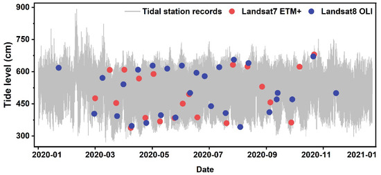
Figure 1.
Tide gauge observations and Landsat overpass data at Cuxhaven in 2020. Red and blue points indicate observation times of Landsat 7 and Landsat 8, respectively.
The number of Landsat observations has increased steadily over time [22]. This higher observation frequency enhances the likelihood of capturing both the highest and lowest tide levels, thereby enabling the detection of larger tidal flat areas. However, excessively dense observations may also lead to an inflation in the long-term tidal flat remote sensing dataset [23], which may cause a spurious increase in mapped tidal flat extent. For instance, Murray et al. [6] mapped the global distribution of tidal flats from 1984 to 2016 and reported that approximately 16.02% of tidal flat loss occurred within only 17.1% of the mapped global tidal flat regions—those with sufficient data to support a consistent multi-decadal time series. In contrast, our statistical analysis of their publicly available dataset reveals an overall increasing trend in global tidal flat area over the past 30 years (as shown in Figure 2), which contradicts their conclusion. This discrepancy between remote sensing-derived statistics and the tidal flat change trends reported may be attributed to the influence of Landsat observation frequency on long-term tidal flat monitoring. Therefore, it is essential to investigate whether the observed increase in tidal flat area reflects a genuine environmental trend or an artifact driven by variations in Landsat observation frequency.
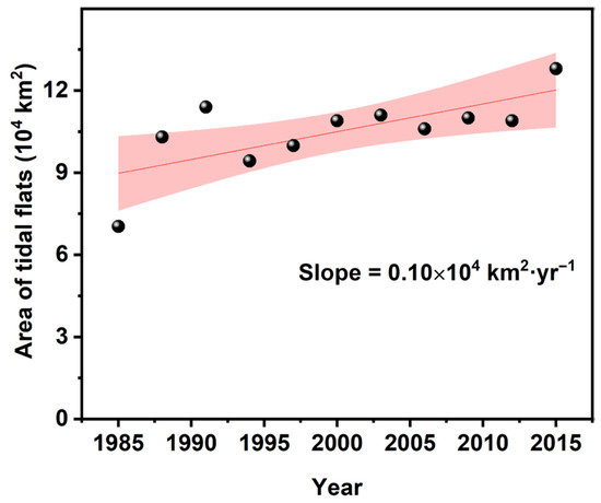
Figure 2.
Global tidal flat area change trend from 1984 to 2016 from Murray’s global tidal flat products.
To address this issue, our study aims to systematically investigate the impact of increased Landsat observation frequency on the long-term mapping of tidal flats, and to quantify both the extent and uncertainty of this influence. First, we selected two widely used long-term global tidal flat datasets (Murray’s tidal flat products [5] and GTF30 produced by Zhang [7]) as the targets, and determined the clear-sky Landsat observation frequencies and tide gauge records at 45 tidal stations. Second, we employed the linear regression method to explore the relationships among observation frequency, tide level, and tidal flat area. Specifically, this study investigated how Landsat observation frequency affects the performance of capturing tide levels and mapping tidal flat areas, as well as the correlation between observation frequency and tide levels. Finally, we developed a weighted statistical regression method to quantify the impact of Landsat observation frequency on Landsat-based tidal flat area mapping and its uncertainty. This approach enables the quantification of the magnitude and uncertainty of observation frequency effects on tidal flat dynamics monitoring, thereby providing a scientific basis for more accurate interpretation of long-term tidal flat trends and ecological assessments.
2. Materials and Methods
2.1. Datasets and Preprocessing
2.1.1. Tide Level Observation Dataset
The UHSLC tide level dataset (https://www.ncei.noaa.gov/access/metadata/landing-page/bin/iso?id=gov.noaa.nodc:JIMAR-JASL, accessed on 20 August 2024), provided by the University of Hawaii Sea Level Center, is a key component of the Global Sea Level Observing System (GLOSS) data stream. While the dataset comprises a wide array of tide gauge records, its core is the GLOSS Core Network (GCN), which consists of approximately 300 tide gauge stations strategically distributed around the globe. This network is designed to offer broad spatial coverage and to ensure an even sampling of coastal sea level variations across diverse regions and timeframes, thereby facilitating comprehensive assessments of both long-term and regional sea level trends. The UHSLC provides tide gauge data with two levels of quality control: Fast Delivery (FD) data, which enables rapid access, and Research Quality Data (RQD), which undergoes more extensive filtering and validation to achieve higher accuracy, albeit with a longer processing time. For the purposes of this study, the more accurate RQD dataset was selected. A total of 147 tide gauge stations were included, with data spanning the years 2000 to 2022. Each station provides measurements at a 1 h temporal resolution, offering detailed temporal information for analyzing tide level fluctuations and changes over the selected period.
Human activities (such as conversion to agriculture or restoration of lost wetlands) have a significant impact on the loss and gain of tidal flats [11], and existing studies have shown that 27% of the loss and gain of tidal flats are related to direct human activities. This study mainly aims to explore the impact of satellite observation frequency on tidal flat changes. Therefore, it is necessary to exclude tidal stations strongly influenced by human activities. Specifically, the tidal flat maps of each period of the long-term tidal flat products were first spatially superimposed to obtain the range of tidal flat changes. The tidal flat changes were then spatially superimposed with the land cover product (GLC_FCS30D by Zhang et al. [24]) to obtain the amount of tidal flat changes affected by human activities (such as conversion to artificial aquaculture pond, urban land, or restoration of lost tidal flats). Their proportion of the tidal flat changes due to human activity was calculated within the 1° grid range of the tidal observation station. If the tidal flat changes by human activity accounted for more than 5% within the 1° grid range of the tidal observation station, these tide stations were discarded. After this optimization, a total of 45 tidal stations were selected, which is illustrated in Figure 3.
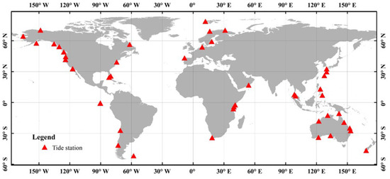
Figure 3.
Spatial distribution of the selected tide stations from UHSLC.
2.1.2. Landsat Data and Tide Levels During Satellite Overpasses
To capture detailed tide information as comprehensively as possible, both long-term tidal flat products utilized all available Landsat imagery from the respective mapping years, including data from Landsat 5 TM, Landsat 7 ETM+, and Landsat 8 OLI. In this study, we selected two long-term tidal flat products from the same mapping years and collected all available Landsat images they used in tidal flat mapping from 2000 to 2022. The “bad-quality” pixels (for example, clouds, cloud shadows, ice and snow, and saturated pixels) will affect tidal flat mapping and are considered polluted pixels. They were masked using the CFmask algorithm [25]. We counted all clear-sky Landsat images of each tidal flat product after masking processing on the public and free cloud computing platform Google Earth Engine (GEE) as the satellite observation frequency of each epoch. Figure 4 shows the spatiotemporal distribution of available Landsat observations at the tide gauge stations. It can be observed that most stations have enough valid Landsat observations and that the total volume of observations has increased over time. Moreover, because tide levels in intertidal zones can fluctuate rapidly throughout the day, and satellite imagery represents only an instantaneous snapshot, it is essential to determine the tide level at the satellite overpass. To achieve this, we recorded the acquisition time of each Landsat observation associated with the tidal flat products during each period. Tide gauge stations provide tide level measurements at an hourly interval, offering high temporal resolution for tide level estimation. We applied a nearest-neighbor matching method to compare the Landsat observation times with the corresponding hourly tide gauge records, thereby obtaining the tide level information at the time of satellite overpass.
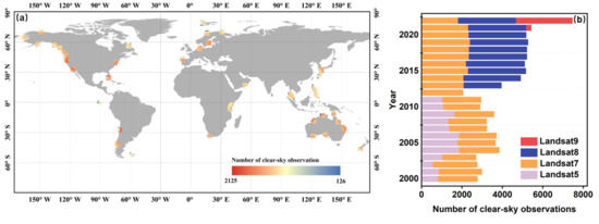
Figure 4.
The spatiotemporal distribution of available Landsat observations at the tide gauge stations. (a) Spatial distribution of the total number of clear-sky Landsat observations at each tide gauge station from 2000 to 2022. (b) Temporal trend of the total number of clear-sky Landsat observations across all tide gauge stations from 2000 to 2022.
2.1.3. Global Long-Term Tidal Flat Products
The global long-term tidal flat dataset released by Murray et al. [6] covers the area between 60°N and 60°S. It integrates a global training dataset of tidal flat distribution, time-series Landsat imagery, 56 spectral predictor variables, and a random forest classification algorithm to produce global tidal flat maps across 11 time periods from 1984 to 2016, with three-year intervals. Accuracy assessment using 1358 validation points indicated an overall accuracy of 82.3%. This dataset is freely available at https://www.intertidal.app/, accessed on 5 September 2024.
To fill the gap in high-latitude tidal flat data, Zhang [7] released a global tidal flat dataset covering high latitudes (>60°N) at 30 m (GTF30) in 2020. They proposed a new spectral index called the LTideI index, which is robust and can accurately capture low tide information. Then, they designed an automatic approach to extract the globally distributed training samples based on multi-source datasets. Finally, they used a local adaptive classification strategy to generate the global tidal flat dataset on the Google Earth Engine platform based on time-series Landsat images in 2020. GTF30 was validated using 13,994 verification samples with an overall accuracy of 90.34%. More recently, Zhang [26] extended GTF30 to an annual product covering 2000 to 2022, which is freely available at https://doi.org/10.5281/zenodo.10068479.
Previous studies have demonstrated that tide level observations at tide gauge stations are highly correlated with regional tidal dynamics, typically within a 1° radius (~100 km) [27]. The spatial coherence of tidal constituents ensures that station-based tide records are representative of the surrounding intertidal environments [28,29]. Therefore, we calculated the tidal flat area within a 1° spatial buffer centered on each tide gauge station using two long-term tidal flat products. We then applied simple linear regression to analyze temporal trends in tidal flat area across all stations in both products.
2.2. Method
This study systematically evaluated the impact of the satellite observation frequency on mapping the long-term change in tidal flat area at the global scale by integrating multi-source remote sensing and tide records. The research framework includes the following three core modules (Figure 5). Firstly, the satellite observation frequency, tide level, and flat tidal area of the selected tide stations over the period of 2000–2020 were calculated from the multi-resource datasets, including the cloud-free Landsat images on the GEE platform, UHSLC tide level dataset, and global tidal flat datasets (GTF30 and Murray’s product). Then, the linear regression method was employed to quantify the relationship between the satellite observation frequency, tide level at satellite overpass, and tidal flat area at the selected tide station. Finally, combined with the temporal trend of the tidal flat area of all stations and the temporal trend of the observation frequency of all stations, the impact of the satellite observation frequency on the tidal flat area of the two long-term tidal flat products, as well as their uncertainty, was obtained.
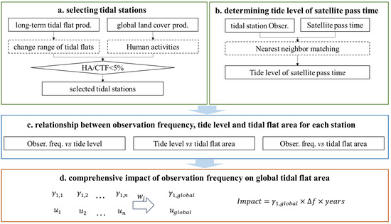
Figure 5.
Flowchart of quantifying the impact of increased satellite observation frequency on the long-term tidal flat area changes.
2.2.1. Temporal Trend Analysis of Satellite Observation Frequency and Mapped Tidal Flat Area
To investigate temporal trends in satellite observation frequency and the mapped tidal flat area, we conducted a systematic trend analysis to evaluate long-term changes under both Landsat observational conditions and tidal flat mapping products. For observation frequency, we quantified the annual number of cloud-free Landsat images available within a 1° spatial buffer surrounding each tide gauge station. These data were used to examine temporal variations in satellite observation availability. Concurrently, to assess changes in tidal flat extent, we extracted annual tidal flat area estimates from two widely used global tidal flat products within the same 1° buffer zones around all stations. We applied simple linear regression models separately to the time series of observation frequency and tidal flat area to quantify their respective trends over time. The slope of the regression line indicates the direction and magnitude of change, while the statistical significance of the model evaluates the reliability of the observed trend. This analysis aims to determine whether the increasing availability of Landsat observations has contributed to systematic changes in the mapped tidal flat area, thereby laying the foundation for subsequent uncertainty assessment and causal inference.
2.2.2. Linear Regression Analysis of Satellite Observation Frequency, Tide Level at Satellite Overpass and Tidal Flat Area
There is a close relationship between the frequency of satellite observations, the tide levels at the time of satellite overpass, and the area of tidal flats monitored by satellites. Specifically, an increase in satellite observation frequency enhances the likelihood of capturing lower tide levels, which in turn increases the probability of observing larger tidal flat areas. This suggests that higher observation frequency may indirectly contribute to a more comprehensive mapping of tidal flats. To quantitatively assess the driving effect of observation frequency on the mapped tidal flat area, this study employs linear regression models at each selected tide station. Three regression analyses were conducted: (1) between satellite observation frequency and tide level at overpass time, (2) between tide level and the monitored tidal flat area, and (3) between satellite observation frequency and the mapped tidal flat area. These models aim to evaluate the influence of satellite observation frequency on tidal flat measurements across varying tide regimes.
The corresponding regression models are defined as follows:
where , and represent the tide level at satellite overpass (cm), the satellite observation frequency (number of valid observations), and the mapped tidal flat area (km2), respectively; , , and are the regression slopes of against , against , and against , respectively; , , and are the corresponding regression intercepts.
In addition, to assess the uncertainty associated with each linear regression model, a residual-based uncertainty metric was applied. This metric estimates the dispersion of fitted values around the observed data and accounts for the effect of sample size [30,31]. The uncertainty was calculated using the following formula:
where is the standard uncertainty of the regression model, is the number of observations, is the observed value of the dependent variable for the i-th data point, and is the corresponding fitted value estimated by the regression model.
The above formulation was applied separately to each of the three regression models, using their respective dependent variables (i.e., tide level, tidal flat area).
2.2.3. Quantifying the Impact of Satellite Observation Frequency on the Mapped Tidal Flat Area at the Global Scale
Recognizing the necessity for a consistent, global-scale assessment that accounts for spatial heterogeneity among tide stations and differing observational conditions, this study introduces an area-weighted hierarchical regression framework to quantify the impact of satellite observation frequency on the mapped tidal flat area and its uncertainties. Initially, for each tide station, a linear regression model is established to derive site-specific regression parameters between satellite observation frequency and the mapped tidal flat area, notably the slope (denoted as ), the uncertainty () and the coefficient of determination (). These parameters, respectively, quantify the sensitivity, reliability, and explanatory power of the model at each individual station. Then, to synthesize this station-specific information into a comprehensive global perspective, we assigned each station a weight coefficient according to its tidal flat area, which is defined as the ratio of its tidal flat area to the total tidal flat area of all stations. Using these weights, the global regression parameters—namely, the globally weighted slope (), weighted (), and weighted ()—are computed to reflect the comprehensive influence of satellite observation frequency across the entire study domain. Formally, the calculations are as follows:
where , and are the slope, uncertainty, and value of the regression model at the -th tide station, respectively; is the number of the selected tidal stations, which equals 45. The weight for each station is determined by the ratio of the tidal flat area at that station to the total tidal flat area summed across all stations, i.e.,
where is the average intertidal area within the 1° grid cell corresponding to each station, which is calculated based on multi-year observations.
Finally, the quantitative impact of satellite observation frequency on the mapped tidal flat area was calculated according to the globally weighted . The impact of satellite observation frequency on the mapped total flat area can be calculated as,
where is the annual average increase in cloud-free satellite observations for all selected tide stations over the period for the long-term global tidal flat dataset.
3. Results
3.1. Trend of Tidal Flat Area Changes
Figure 6 presents the spatial distribution and long-term trends of tidal flat area changes over time for both the GTF30 and Murray’s tidal flat products across all selected tide stations. Both products exhibit an overall increasing trend in tidal flat area at these locations, as illustrated by the temporal trajectories in Figure 6c,e. However, the extent of this increase differs notably between the two. Specifically, the GTF30 product shows a total increase of 73.04 km2 in tidal flat area across the selected stations, accounting for 1.71% of the total tidal flat area in 2020. In comparison, Murray’s product exhibits a much smaller increase of only 7.13 km2, representing 0.35% of the 2020 total. Spatial analysis of both the absolute area and the magnitude of change across tide stations (Figure 6a,b) indicates that the tidal flat areas identified by GTF30 are generally larger than those from Murray’s product at most locations. Notably, in Murray’s product, increases in tidal flat area tend to be concentrated in regions that already possess extensive tidal flats. In contrast, the GTF30 product reveals that regions with initially large tidal flat extents not only experienced significant growth, but even areas with relatively small initial extents also exhibit an increasing trend. Moreover, as shown in Figure 6d, the total number of Landsat observations at all tide stations has exhibited a marked upward trend over time, particularly following the launch of Landsat 8 in 2013, with an average annual increase of approximately five cloud-free observations. This increasing frequency of satellite observations may partly account for the observed expansion of tidal flat area in both products, suggesting an inflation in the mapping outcomes.
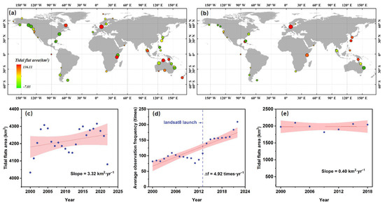
Figure 6.
The spatial distribution and overall temporal trends of tidal flat area changes at all selected tide stations for both tidal flat products. (a,b) The spatial distribution of tidal flat areas and their changes for the GTF30 and Murray’s products, respectively, across the selected tide stations. The size of each circle represents the average tidal flat area at a given station over the past 20 years, while the color of the circle reflects both the direction and magnitude of change in tidal flat area during this period. (c,e) The temporal trends in the total tidal flat area across all selected tide stations for the GTF30 and Murray’s products, respectively. (d) The temporal trend in Landsat observation frequency at all selected tide stations.
3.2. The Relationship Among Observation Frequency, Tide Level, and Tidal Flat Area
Figure 7 presents boxplots of observed tide levels at two tide gauge stations, overlaid with the distribution of tide levels at satellite overpass. The analysis indicates that higher satellite observation frequency corresponds to a larger range of tide level variation. This is reflected in the denser distribution of tide levels at satellite overpass within the boxplots, which also include values approaching the extreme conditions—namely, the highest and lowest tide levels. Notably, tide levels at stations with more frequent observations are closer to the actual peak and nadir tide levels recorded by tide gauges. These findings suggest that higher observation frequency improves the capability of satellites to capture the full range of tide variability, thereby reducing the sampling bias associated with lower-frequency observations.
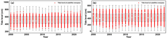
Figure 7.
Distribution of tide levels at satellite overpass relative to observed tide levels at typical tide gauge stations from 2000 to 2022. Station (a): Cuxhaven station; Station (b): Darwin station.
To quantify the influence of observation frequency on the ability to capture tide extremes, this study further computed the percentile ranks of the maximum and minimum tide levels at satellite overpass relative to the full distribution of observed tide levels at each station. This metric reflects the extent to which satellite observations can represent the extreme states of the tide. For instance, at the tide station shown in Figure 7a, the percentile rank of the lowest tide levels at satellite overpass improved from the 1.95 percentile to the 0.70 percentile as observation frequency increased. Similarly, at the station shown in Figure 7b, this value improved from the 7.84 percentile to the 2.59 percentile with increased observation frequency. Overall, the results indicate that denser satellite observation schedules significantly enhance the probability of capturing tide extremes, thereby enabling a more accurate and comprehensive representation of tidal dynamics.
Figure 8 presents satellite-derived imagery capturing the lowest and highest tide levels at two representative tide stations in 2020, along with the temporal trends in both the observed lowest tide levels at satellite overpass times and the corresponding tidal flat areas within a 1° buffer around each station. It is evident that satellites detect a much broader extent of tidal flats during low tide conditions (Figure 8a,d), while during high tide, the detectable extent becomes markedly smaller (Figure 8b,e). This spatial contrast highlights the substantial influence of tidal variation on the observable geomorphic extent of tidal flats, particularly in regions experiencing greater tide amplitude. Furthermore, the analysis of temporal trends (Figure 8c,f) reveals a strong association between the mapped tidal flat area and the lowest tide levels at the time of satellite overpass. Specifically, an increase in the observed tidal flat area corresponds with a decreasing trend in the lowest tide levels, and stations experiencing greater reductions in tide level tend to show more substantial increases in mapped tidal flat areas. These findings emphasize the critical link between tidal conditions and the spatiotemporal variability of satellite-derived tidal flat extents.
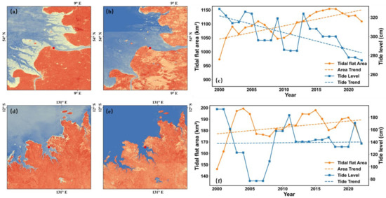
Figure 8.
Satellite-derived imagery of the lowest and highest tide levels in 2020 at two representative tide stations, along with the temporal trends (2000–2022) of tidal flat area and the lowest tide level at satellite overpass times within a 1° buffer around each station. (a,b) The lowest and highest tide level images at the Cuxhaven station, respectively. (d,e) The corresponding images at the Darwin station. (c,f) The temporal trends of tidal flat area and the lowest tide level at satellite overpass times for the Cuxhaven and Darwin stations, respectively.
Figure 9a presents box plots of the R2 values derived from the GTF30 and Murray tidal flat products for all 45 stations from 2000 to 2022. For the relationship between observation frequency and tide level, the GTF30 product showed an R2 () of 0.18, suggesting a limited ability of observation frequency to explain tide level variability. In comparison, the Murray product showed a slightly higher R2 () of 0.22, indicating a marginally stronger association. This limited correlation can be explained by the periodic nature of tide levels and the fixed satellite overpass schedule, which constrains the ability of satellites to capture tides at different phases. Consequently, even in regions with high observation frequency, the temporal mismatch prevents full coverage of tide variability, limiting the correlation between observation frequency and tide level. Similarly, for the regression between tide level and tidal flat area, the R2 () values were 0.18 and 0.23 for the GTF30 and Murray products, respectively. These results suggest that while tide level does affect the extent of tidal flats, it alone cannot fully explain the variations. This limited explanatory power can be attributed to the inherent complexities of local topography, geomorphic features, and other environmental factors. Moreover, tide level is only one of several important parameters influencing the generation of tidal flat products. Based on the significant increase in satellite observation frequency after the launch of Landsat 8, shown in Figure 6d, we further analyzed the distributions of R2 derived from the regression models between observation frequency, tide level, and tidal flat area for the periods before and after the Landsat 8 launch (Figure 9b,c). Both tidal flat products exhibit higher R2 in the post-Landsat 8 period compared with the earlier years, and the improvement is more pronounced for Murray’s product. This suggests that the Murray dataset may be more sensitive to variations in tidal flat area driven by changes in observation frequency and tide level under conditions of enhanced observation availability. As a result, although the relationship between satellite observation frequency and mapped tidal flat area is statistically significant, the associated uncertainty remains substantial—approximately 50% based on Equations (4) and (6). Combining these observations, it becomes evident that higher observation frequency increases the likelihood of capturing lower tide conditions, which in turn exposes more tidal flats during imaging. Therefore, stations with more satellite observations tend to record larger tidal flat areas. This mechanism quantitatively links observation frequency, tide level, and mapped tidal flat extent, providing a statistical basis for the observed increase in detected tidal flats with higher observation frequency.
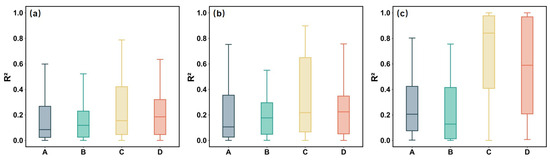
Figure 9.
Distribution of R2 values from regression models relating observation frequency, tide level, and tidal flat area for two global tidal flat products across different time periods. (a) R2 distributions for 2000–2022. (b) R2 distributions for 2000–2012 (before the launch of Landsat 8). (c) R2 distributions for 2013–2022 (after the launch of Landsat 8). A: GTF30, observation frequency vs. tide level; B: GTF30, tide level vs. tidal flat area; C: Murray, observation frequency vs. tide level; D: Murray, tide level vs. tidal flat area.
3.3. The Relationship Between Observation Frequency and Tidal Flat Area
The average increase in satellite cloud-free observation for the selected 45 stations during the period 2000–2020 is 4.92 times·yr−1. Such growth in satellite observation frequency would lead to an inflated increase in global tidal flat area. A comprehensive linear regression analysis was conducted to examine the relationship between the satellite observation frequency and the tidal flat area in the GTF30 product at all selected stations. The results, presented in Figure 10a,b, depict the linear regression relationships between observation frequency and tidal flat area for two representative stations, providing an intuitive visualization of their correlation. Additionally, Figure 10c systematically summarizes the three regression parameters—specifically, slope (), (), and ()—for all selected tide stations, offering an overarching perspective on the relationships across different stations, with an average slope () of 0.13 km2/times, () of 0.21, and uncertainty () of 50.75%. This indicates that for each increase in observation frequency, the tidal flat area increases by approximately 0.13 km2 on average. However, the relatively low R2 value suggests that other factors or sources of variability may influence this relationship.
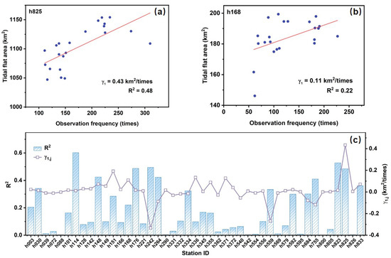
Figure 10.
Linear regression slope and R2 between observation frequency and tidal flat area at stations in the GTF30 product. (a,b) The linear regression results of observation frequency and tidal flat area for the Cuxhaven and Darwin stations, respectively; (c) The regression slopes and R2 values for all stations.
According to the area-weighted regression model presented in Equations (6) and (9), the influence of satellite observation frequency on tidal flat area over the past two decades was quantified as 12.83 ± 6.51 km2. Considering that the total growth of the tidal flat area of the selected 45 stations in the GTF30 product is 73.04 km2, approximately 17.57% of this increase can be attributed to the growth in satellite observation frequency over the past two decades. Such a spurious increase due to the increased satellite observations corresponds to about 0.30% of the total tidal flat area of the selected 45 tide stations in 2020.
A similar regression analysis was performed using the Murray intertidal product for the 45 selected tide stations. The analysis yielded an average slope () of 0.14 km2/times, () of 0.30, and uncertainty () of 53.53%. This indicates that for each increase in observation frequency, the tidal flat area increases by approximately 0.14 km2 on average. Based on the area-weighted regression model described in Equations (6) and (8), the estimated impact of increased satellite observation frequency on tidal flat area over the past two decades was 13.92 ± 7.45 km2. However, the actual increase in mapped tidal flat area among the 45 selected stations in the Murray product during the same period was only 7.13 km2. This implies that the estimated effect of observation frequency exceeds the observed area change by approximately 95.23%, suggesting that the apparent expansion is largely attributable to increased satellite observations rather than actual environmental change. The pseudo-expansion caused by increased observation frequency accounts for approximately 0.68% of the total mapped tidal flat area at the 45 stations in 2020.
4. Discussion
4.1. Uncertainty in the Algorithm Principle of Tidal Flat Products
This study reveals the relationship between satellite observation frequency and variations in tidal flat area. Although existing tidal flat mapping algorithms (e.g., the global products developed by Murray et al. [5] and Zhang et al. [26]) are not solely based on low-tide information, the capture of low-tide conditions is an essential component embedded in their designs. For instance, Murray’s product employs a random forest classifier trained with manually labeled low-tide samples from multi-temporal Landsat images, and incorporates various spectral and water indices through multiple temporal compositing approaches (mean-interval, max–min, median, quantile, and standard deviation) [6]. These procedures enhance sensitivity to observation frequency, as the inclusion of more scenes leads to greater spectral variability across composite features. In contrast, Zhang’s GTF30 product uses automatically generated global training samples and a local adaptive classification strategy. By introducing the LTideI index and employing its maximum composite to represent the lowest-tide exposure [7], GTF30 achieves a more stable depiction of tidal flats, reducing the algorithm’s dependence on observation frequency. These algorithmic differences ultimately influence how each product responds to variations in satellite observation frequency, which further shapes the spatial patterns and magnitudes of the mapped tidal flat area.
However, the irregularity and incompleteness of low-tide capture due to spatiotemporal heterogeneity in satellite observation frequency—particularly in regions with persistent cloud cover, short low-tide durations, or low revisit rates—can lead to systematic underrepresentation of the actual tidal flat area [32,33]. In such scenarios, the mapping algorithm may fail to detect the true boundary of the intertidal zone, especially the most seaward extent, which only becomes visible during extreme low tides. This deficiency introduces bias and contributes to the uncertainty in the final tidal flat product. Our findings further confirm this relationship: a statistically significant negative correlation between satellite observation frequency and the range of tide level variation (ΔH) indicates that higher-frequency observations are more likely to capture lower tide stages. This relationship supports the notion that frequent observations improve the temporal coverage of low-tide events, thereby increasing the probability of detecting the maximum tidal flat exposure. As a result, regions with higher observation frequencies tend to yield larger mapped tidal flat areas, not necessarily due to environmental change, but due to enhanced visibility of the actual intertidal extent.
Nevertheless, current algorithms do not fully isolate the effects of tidal dynamics from other co-varying environmental drivers. Factors such as sediment transport [34], seasonal vegetation phenology (e.g., salt marshes or mangroves) [35], and water turbidity may confound the spectral signals used in classification or index-based methods. This coupling of tidal and non-tidal influences complicates the interpretation of the observed area dynamics and may obscure the true impact of tidal stage variability. Moreover, the static treatment of tidal influence in many models—where tidal level is not dynamically incorporated into the mapping logic—limits their adaptability across regions with diverse tidal regimes [32]. For example, macrotidal zones may experience more frequent exposure opportunities, while microtidal regions require high-temporal-resolution data to reliably detect episodic low-tide conditions [36]. Without explicit modeling of these hydrodynamic differences, the mapping algorithm may underperform in certain geographic contexts.
To reduce these uncertainties, future research should aim to explicitly integrate tidal modeling into the classification or segmentation process, for example, by incorporating predicted tidal levels at the time of image acquisition using tidal models (e.g., FES2014, TPXO). In addition, combining multi-source satellite data with varying temporal resolutions (e.g., Sentinel-2, Planet Scope, or SAR-based datasets) could improve the temporal sampling of low-tide conditions.
4.2. Uncertainty in the Satellite-Captured Tide Level
The uncertainty in this study primarily arises from the inherent limitations of satellite-based observations, the complex and non-linear interactions between tidal levels and intertidal surface dynamics, as well as the limited global representativeness of the selected tide gauge stations. Recognizing the constraints of using remote sensing to characterize tidal extremes is essential for accurately interpreting tidal flat area changes and ensuring the reliability of spatiotemporal analyses.
First, the ability of satellites to effectively capture extreme low-tide events is fundamentally constrained by the temporal characteristics of satellite overpasses and the astronomical and geomorphological drivers of tidal dynamics. For example, optical satellites such as Landsat typically acquire imagery at fixed local solar times (e.g., ~10:30 a.m.), whereas the timing of astronomical low tides varies throughout the lunar cycle due to the combined effects of lunar-solar gravitational interactions, Earth’s axial tilt, and coastal morphology. This mismatch in timing—referred to as temporal aliasing—means that satellites may repeatedly miss the precise windows of extremely low-tide exposures, even in regions with relatively high observation frequencies. Consequently, there exists an intrinsic ceiling to the potential correlation between observation frequency and the probability of capturing the lowest tide levels. This phenomenon has been observed in various tidal regimes, where consistently high revisit rates fail to yield proportional improvements in low-tide detection.
Second, the relationship between the lowest observed tide and the extent of exposed tidal flats is influenced by multiple environmental factors that can obscure or disrupt this correlation. While lower tidal levels theoretically correspond to a greater extent of exposed intertidal surfaces, this idealized relationship can be significantly altered by transient hydrodynamic processes (e.g., storm surges, wind-driven waves), surface characteristics (e.g., sediment compaction, algal blooms), and longer-term morphological changes such as erosion, accretion, or vegetation encroachment [37]. For instance, at certain stations, even when the satellite captured an expected low-tide window, the observed tidal flat area was reduced due to sediment resuspension that increased water turbidity, or seasonal macroalgal blooms that obscured the true boundary of the intertidal zone in the spectral imagery. These factors introduce nonlinearity and hysteresis into the area–tide relationship, weakening the statistical association and reducing the predictive value of low-tide detection for tidal flat mapping. To address these challenges, future research should prioritize the integration of complementary data sources and the development of physically informed models [14,38]. For instance, synthetic aperture radar (SAR) imagery—unaffected by cloud cover and capable of capturing surface roughness and moisture differences—can be used to improve low-tide detection, particularly in regions where optical imagery is compromised.
Furthermore, the global representativeness of the 45 tide gauge stations used to assess the influence of satellite observation frequency on tidal flat area remains limited. We excluded stations strongly affected by human activities; however, this filtering also removed many stations that combine substantial natural tidal flat variability with anthropogenic disturbances—such as the extensive tidal flats along the Yellow Sea—which may introduce bias into global estimates. In addition, macrotidal and microtidal environments are not evenly sampled, and environmental differences among stations (tidal range, sedimentary regime, coastal morphology) may affect the transferability of our results. These limitations imply that the global applicability of the inferred inflation factor requires further evaluation with more spatially and morphodynamically diverse stations.
Although this study focuses on tidal flats, the effects of satellite observation frequency may also apply to beaches and other coastal types. High-frequency observations are important for capturing dynamic changes such as shoreline retreat, seasonal variability, and morphological adjustments. In future coastal zone research using long-term Landsat data, variations in observation frequency should be carefully considered, as they may introduce apparent or artificial changes in the mapped tidal flat area. To reduce such biases, future studies are encouraged to normalize or correct for observation frequency effects, integrate complementary datasets such as SAR imagery to address temporal gaps, and incorporate seasonal and geomorphic context to distinguish genuine environmental changes from observation-related variability. These efforts would improve the robustness and reliability of long-term coastal change assessments.
5. Conclusions
With advancements in remote sensing data acquisition capabilities, the number of available satellite observations has grown significantly over the past two decades. Tidal flats, as a highly dynamic land cover type affected by tides, may appear inflated when mapped using denser satellite observations. This study systematically evaluated the driving mechanism and impact of the satellite observation frequency on the change in tidal flat area at the global scale by integrating tide measurements and multi-source remote sensing and measured data, including two popular long-term tidal flat datasets (GTF30 and Murray’s product). The results show that satellite observation frequency has a significant influence on tidal flat area changes in the selected tide stations. There is a spurious increase of approximately 12.83 ± 6.51 km2 attributed to the growth of satellite observation frequency in the GTF30 dataset, representing 0.30% of the total tidal flat area and 17.57% of the total change in tidal flat area. For Murray’s dataset, the spurious increase in tidal flat area attributed to the growth in satellite observation frequency is approximately 13.92 ± 7.45 km2, accounting for 0.68% of the total tidal flat area and being approximately 1.95 times the actual change in the tidal flat area. Therefore, the inflated increase in tidal flat area in the long-term global dataset attributable to increased observation frequency needs to be quantified, which is essential for accurate interpretation of the long-term tidal flat dynamics and ecological assessments.
Author Contributions
Conceptualization, L.L., J.W. and X.Z.; methodology, L.L., J.W., X.Z. and T.Z.; funding acquisition, L.L. and X.Z.; writing—original draft, J.W. and X.Z.; writing—review and editing, J.W., X.Z. and L.L. All authors have read and agreed to the published version of the manuscript.
Funding
This study is financially supported by the National Key Research and Development Program of China [Grant No. 2023YFB3907403].
Data Availability Statement
The global long-term tidal flat products and tide station data covered in this study are freely available online from their distributing organizations.
Acknowledgments
The authors would like to thank all producers of publicly available global long-term tidal flat products and tide station data.
Conflicts of Interest
The authors declare no conflicts of interest.
References
- Brockmann, C.; Stelzer, K. Optical Remote Sensing of Intertidal Flats. In Remote Sensing of the European Seas; Barale, V., Gade, M., Eds.; Springer: Dordrecht, The Netherlands, 2008; pp. 117–128. [Google Scholar]
- Barbier, E.B.; Koch, E.W.; Silliman, B.R.; Hacker, S.D.; Wolanski, E.; Primavera, J.; Granek, E.F.; Polasky, S.; Aswani, S.; Cramer, L.A.; et al. Coastal Ecosystem-Based Management with Nonlinear Ecological Functions and Values. Science 2008, 319, 321–323. [Google Scholar] [CrossRef] [PubMed]
- Bell, P.S.; Bird, C.O.; Plater, A.J. A temporal waterline approach to mapping intertidal areas using X-band marine radar. Coast. Eng. 2016, 107, 84–101. [Google Scholar] [CrossRef]
- Murray, N.J.; Clemens, R.S.; Phinn, S.R.; Possingham, H.P.; Fuller, R.A. Tracking the rapid loss of tidal wetlands in the Yellow Sea. Front. Ecol. Environ. 2014, 12, 267–272. [Google Scholar] [CrossRef]
- Murray, N.J.; Phinn, S.P.; Fuller, R.A.; DeWitt, M.; Ferrari, R.; Johnston, R.; Clinton, N.; Lyons, M.B. High-resolution global maps of tidal flat ecosystems from 1984 to 2019. Sci. Data 2022, 9, 123–138. [Google Scholar] [CrossRef] [PubMed]
- Murray, N.J.; Phinn, S.R.; DeWitt, M.; Ferrari, R.; Johnston, R.; Lyons, M.B.; Clinton, N.; Thau, D.; Fuller, R.A. The global distribution and trajectory of tidal flats. Nature 2019, 565, 222–225. [Google Scholar] [CrossRef]
- Zhang, X.; Liu, L.Y.; Wang, J.Q.; Zhao, T.T.; Liu, W.D.; Chen, X.D. Automated Mapping of Global 30-m Tidal Flats Using Time-Series Landsat Imagery: Algorithm and Products. J. Remote Sens. 2023, 3, 0091. [Google Scholar] [CrossRef]
- Cao, W.; Zhou, Y.; Li, R.; Li, X. Mapping changes in coastlines and tidal flats in developing islands using the full time series of Landsat images. J. Remote Sens. Environ. 2020, 239, 111665. [Google Scholar] [CrossRef]
- Zhang, M.; Lang, Z.; Liu, Y. Variation mechanisms of suspended sediment concentration in complex estuary determined through remote sensing, observation and modeling coupling. J. Int. J. Appl. Earth Obs. Geoinf. 2025, 139, 104539. [Google Scholar] [CrossRef]
- Xu, C.; Liu, W. Mapping and analyzing the annual dynamics of tidal flats in the conterminous United States from 1984 to 2020 using Google Earth Engine. Environ. Adv. 2022, 7, 100147. [Google Scholar] [CrossRef]
- Murray, N.J.; Worthington, T.A.; Bunting, P.; Duce, S.; Hagger, V.; Lovelock, C.E.; Lucas, R.; Saunders, M.I.; Sheaves, M.; Spalding, M.; et al. High-resolution mapping of losses and gains of Earth’s tidal wetlands. Science 2022, 376, 744–749. [Google Scholar] [CrossRef]
- Wulder, M.A.; Masek, J.G.; Cohen, W.B.; Loveland, T.R.; Woodcock, C.E. Opening the archive: How free data has enabled the science and monitoring promise of Landsat. Remote Sens. Environ. 2012, 122, 2–10. [Google Scholar] [CrossRef]
- Zhao, B.X.; Liu, Y.X.; Wang, L.; Liu, Y.C.; Sun, C.; Fagherazzi, S. Stability evaluation of tidal flats based on time-series satellite images: A case study of the Jiangsu central coast, China. Estuar. Coastal Shelf Sci. 2022, 264, 107697. [Google Scholar] [CrossRef]
- Xu, N.; Wang, L.; Xu, H.; Ma, Y.; Li, Y.; Wang, X.H. Deriving Accurate Intertidal Topography for Sandy Beaches Using ICESat-2 Data and Sentinel-2 Imagery. J. Remote Sens. 2024, 4, 0305. [Google Scholar] [CrossRef]
- Allen, G.H.; Yang, X.; Gardner, J.; Holliman, J.; David, C.H.; Ross, M. Timing of Landsat Overpasses Effectively Captures Flow Conditions of Large Rivers. Remote Sens. 2020, 12, 1510. [Google Scholar] [CrossRef]
- Jia, M.; Wang, Z.; Mao, D.; Ren, C.; Wang, C.; Wang, Y. Rapid, robust, and automated mapping of tidal flats in China using time series Sentinel-2 images and Google Earth Engine. Remote Sens. Environ. 2021, 255, 112285. [Google Scholar] [CrossRef]
- Zhang, Z.; Xu, N.; Li, Y.; Li, Y. Sub-continental-scale mapping of tidal wetland composition for East Asia: A novel algorithm integrating satellite tide-level and phenological features. Remote Sens. Environ. 2022, 269, 112799. [Google Scholar] [CrossRef]
- Wang, X.; Xiao, X.; Zou, Z.; Hou, L.; Qin, Y.; Dong, J.; Doughty, R.B.; Chen, B.; Zhang, X.; Chen, Y.; et al. Mapping coastal wetlands of China using time series Landsat images in 2018 and Google Earth Engine. ISPRS J. Photogramm. Remote Sens. 2020, 163, 312–326. [Google Scholar] [CrossRef]
- Zhang, Y.T.; Woodcock, C.E.; Arevalo, P.; Olofsson, P.; Tang, X.J.; Stanimirova, R.; Bullock, E.; Tarrio, K.R.; Zhu, Z.; Friedl, M.A. A Global Analysis of the Spatial and Temporal Variability of Usable Landsat Observations at the Pixel Scale. Front. Remote Sens. 2022, 3, 894618. [Google Scholar] [CrossRef]
- Zhou, Y.; Dong, J.; Liu, J.; Metternicht, G.; Shen, W.; You, N.; Zhao, G.; Xiao, X. Are There Sufficient Landsat Observations for Retrospective and Continuous Monitoring of Land Cover Changes in China? Remote Sens. 2019, 11, 1808. [Google Scholar] [CrossRef]
- Zhang, X.; Liu, L.Y.; Zhao, T.T.; Gao, Y.; Chen, X.D.; Mi, J. GISD30: Global 30 m impervious-surface dynamic dataset from 1985 to 2020 using time-series Landsat imagery on the Google Earth Engine platform. Earth Syst. Sci. Data 2022, 14, 1831–1856. [Google Scholar] [CrossRef]
- Wulder, M.A.; Loveland, T.R.; Roy, D.P.; Crawford, C.J.; Masek, J.G.; Woodcock, C.E.; Allen, R.G.; Anderson, M.C.; Belward, A.S.; Cohen, W.B.; et al. Current status of Landsat program, science, and applications. Remote Sens. Environ. 2019, 225, 127–147. [Google Scholar] [CrossRef]
- Bayle, A.; Gascoin, S.; Berner, L.T.; Choler, P. Landsat-based greening trends in alpine ecosystems are inflated by multidecadal increases in summer observations. Ecography 2024, 2024, 12. [Google Scholar] [CrossRef]
- Zhang, X.; Zhao, T.; Xu, H.; Liu, W.; Wang, J.; Chen, X.; Liu, L. GLC_FCS30D: The first global 30 m land-cover dynamics monitoring product with a fine classification system for the period from 1985 to 2022 generated using dense-time-series Landsat imagery and the continuous change-detection method. Earth Syst. Sci. Data 2024, 16, 1353–1381. [Google Scholar] [CrossRef]
- Zhu, Z.; Woodcock, C.E. Automated cloud, cloud shadow, and snow detection in multitemporal Landsat data: An algorithm designed specifically for monitoring land cover change. Remote Sens. Environ. 2014, 152, 217–234. [Google Scholar] [CrossRef]
- Zhang, X.; Liu, L.; Zhao, T.; Wang, J.; Liu, W.; Chen, X. Global annual wetland dataset at 30 m with a fine classification system from 2000 to 2022. Sci. Data 2024, 11, 310. [Google Scholar] [CrossRef]
- Ray, R.D. Precise comparisons of bottom-pressure and altimetric ocean tides. J. Geophys. Res. Oceans 2013, 118, 4570–4584. [Google Scholar] [CrossRef]
- Thompson, P.R.; Mitchum, G.T. Coherent sea level variability on the North Atlantic western boundary. J. Geophys. Res. Oceans 2014, 119, 5676–5689. [Google Scholar] [CrossRef]
- Guo, L.; van der Wegen, M.; Wang, Z.B.; Roelvink, D.; He, Q. Exploring the impacts of multiple tidal constituents and varying river flow on long-term, large-scale estuarine morphodynamics by means of a 1-D model. J. Geophys. Res. Earth Surf. 2016, 121, 1000–1022. [Google Scholar] [CrossRef]
- Niven, E.B.; Deutsch, C.V. Calculating a robust correlation coefficient and quantifying its uncertainty. Comput. Geosci. 2012, 40, 1–9. [Google Scholar] [CrossRef]
- Farrance, I.; Frenkel, R. Uncertainty of Measurement: A Review of the Rules for Calculating Uncertainty Components through Functional Relationships. Clin. Biochem. Rev. 2012, 33, 49–75. [Google Scholar]
- Ma, S.; Wang, N.; Zhou, L.; Yu, J.; Chen, X.; Chen, Y. Inversion of Tidal Flat Topography Based on the Optimised Inundation Frequency Method—A Case Study of Intertidal Zone in Haizhou Bay, China. Remote Sens. 2024, 16, 685. [Google Scholar] [CrossRef]
- Chang, M.; Li, P.; Li, Z.; Wang, H. Mapping Tidal Flats of the Bohai and Yellow Seas Using Time Series Sentinel-2 Images and Google Earth Engine. Remote Sens. 2022, 14, 1789. [Google Scholar] [CrossRef]
- D’Alpaos, A.; Tognin, D.; Tommasini, L.; D’Alpaos, L.; Rinaldo, A.; Carniello, L. Statistical characterization of erosion and sediment transport mechanics in shallow tidal environments—Part 1: Erosion dynamics. Earth Surf. Dynam. 2024, 12, 181–199. [Google Scholar] [CrossRef]
- Wu, W.; Lin, Z.; Chen, C.; Chen, Z.; Zhao, Z.; Su, H. Tracking the dynamics of tidal wetlands with time-series satellite images in the Yangtze River Estuary, China. Int. J. Digit. Earth 2024, 17, 2330684. [Google Scholar] [CrossRef]
- Luan, K.; Wan, H.-F.; Wang, Z.; Lu, X.; Bei, Z.; Yuan, J.; Cao, Z.; You, X.; Wang, J.; Shen, W.; et al. Mapping of Yangtze River Estuary Tidal Flat Based on Sentinel-2 Sensor and Google Earth Engine. Sens. Mater. 2024, 36, 2983–3000. [Google Scholar] [CrossRef]
- Kim, K.; Jung, H.C.; Choi, J.-K.; Ryu, J.-H. Statistical Analysis for Tidal Flat Classification and Topography Using Multitemporal SAR Backscattering Coefficients. Remote Sens. 2021, 13, 5169. [Google Scholar] [CrossRef]
- Pricope, N.G.; Halls, J.N.; Dalton, E.G.; Minei, A.; Chen, C.; Wang, Y. Precision Mapping of Coastal Wetlands: An Integrated Remote Sensing Approach Using Unoccupied Aerial Systems Light Detection and Ranging and Multispectral Data. J. Remote Sens. 2024, 4, 169. [Google Scholar] [CrossRef]


Disclaimer/Publisher’s Note: The statements, opinions and data contained in all publications are solely those of the individual author(s) and contributor(s) and not of MDPI and/or the editor(s). MDPI and/or the editor(s) disclaim responsibility for any injury to people or property resulting from any ideas, methods, instructions or products referred to in the content. |
© 2025 by the authors. Licensee MDPI, Basel, Switzerland. This article is an open access article distributed under the terms and conditions of the Creative Commons Attribution (CC BY) license (https://creativecommons.org/licenses/by/4.0/).