Highlights
What are the main findings?
- A Gradient Boosting Regressor model using Sentinel-2 data accurately predicts turbidity in a dynamic estuary.
- The River Mersey model achieved an R2 of 0.84, demonstrating robustness in complex estuarine environments.
What are the implications of the main findings?
- Machine learning enables scalable, spatially continuous monitoring of water quality in coastal systems.
- This study provides a foundation for future integration of satellite-based ML models with hydrodynamic simulations.
Abstract
The monitoring of turbidity in estuarine environments is a challenging essential task for managing water quality and ecosystem health. This study focuses on the lower reaches of the River Mersey, Liverpool. Harmonized Sentinel-2 MSI Level-2A imagery was integrated with in situ measurements from seven Environment Agency monitoring stations for two consecutive years (January 2023–January 2025). The workflow included image preprocessing, spectral index calculation, and the application of four machine learning algorithms: Gradient Boosting Regressor, XGBoost, Support Vector Regressor, and K-Nearest Neighbors. Among these, Gradient Boosting Regressor achieved the highest predictive accuracy (R2 = 0.84; RMSE = 15.0 FTU), demonstrating the suitability of ensemble tree-based methods for capturing non-linear interactions between spectral indices and water quality parameters. Residual analysis revealed systematic errors linked to tidal cycles, depth variation, and salinity-driven stratification, underscoring the limitations of purely data-driven approaches. The novelty of this study lies in demonstrating the feasibility and proof-of-concept of using machine learning to derive spatially explicit turbidity estimates under data-limited estuarine conditions. These results open opportunities for future integration with Computational Fluid Dynamics models to enhance temporal forecasting and physical realism in estuarine monitoring systems. The proposed methodology contributes to sustainable coastal management, pollution monitoring, and climate resilience, while offering a transferable framework for other estuaries worldwide.
1. Introduction
The sustainable management of freshwater resources is a critical global issue. Despite the fact that water occupies over 70% of the surface areas of the Earth, only 2.5% constitute freshwater, mainly trapped down in glaciers and polar ice caps [1]. Rivers, lakes and estuaries therefore play an important part in the distribution of water for drinking water supply, agriculture and industry, as well as for the maintenance of various ecosystems. Coastal and riverine ecosystems are most vulnerable to degradation from a variety of natural and anthropogenic pressures such as climate change, urbanization and pollution [2]. Turbidity and suspended sediment concentration (SSC) are globally recognized as water quality indices of prime importance to diagnose the health of aquatic ecosystems and the efficacy of water treatment processes [3]. Waterbodies with high turbidity can affect niche quality for fish and other organisms, disrupt drinking water treatment processes and increase the cost of disinfection and treatment by municipalities [4]. In situ turbidity levels are generally measured based on Nephelometric Turbidity Units (NTU) and Formazin Nephelometric Units (FNU) [3]. While traditional methods (similar to fixed stations or boat-ground surveys) give precious data, they are expansive, limited in capturing complex spatial patterns and rapid fluctuations in turbidity [5,6].
In contrast, remote sensing has been developed as an important complementary tool for long-term and large-scale turbidity monitoring with various resolutions [3]. Multispectral satellite detectors, similar to Sentinel-2 and Landsat 8, offer the spatial and temporal content demanded to detect changes in turbidity over large areas at regular intervals, which heavily rely on green, red-edge, NIR, and SWIR bands [5,7]. Spectral indicators such as the Normalised Difference Turbidity Index (NDTI) [8], Normalised Difference Vegetation Index (NDVI) [9], Total Suspended Solids Index (TSSI) [10] and other band rates sensitive to suspended sediments [11,12], estimate turbidity patterns that would be difficult to capture with traditional point sampling alone. Nonetheless, converting satellite-derived reflectance into accurate turbidity values requires robust estimation using in situ data and frequently benefits from advanced logical methods, similar to Machine Learning (ML) [6].
Suspended particles, which include sediments, organic matter, and pollutants, are the primary drivers of water clarity [4]. The complex relationship between turbidity, chlo-rophyll-a (Chl-a), and total suspended matter (TSM) means that changes in one can have non-obvious effects on the others, especially in optically complex waters [13,14]. Advanced analytical methods, such as machine learning compare and evaluate satellite reflectance algorithms, offer a powerful way to model these non-linear relationships [14,15]. However, these algorithms are highly dependent on the data availability and level of accuracy, which emphasizes the sensitivity of selecting a suitable atmospheric correction method [16]. The harsh reflectance could propagate errors into an ML-based model, thereby reducing the accuracy of predictions by multiplying errors into the model [6].
By integrating remote sensing, machine learning, and ground truth data, it becomes possible to create high-resolution turbidity maps and develop dependable forecasts for complex terrains like the River Mersey, an urban estuary in northwest England. The River Mersey has long faced challenges related to industrial discharges and sediment transport dynamics [17]. Moreover, current maritime infrastructure and renewable energy projects, such as dredging, tidal turbine installation, harbour upgrades, and other activities, pose additional risks of sediment disturbance to assess variations in environmental impacts [18]. However, despite improvements in remote sensing and Machine Learning for water quality analysis, there remains a lack of research that specifically integrates these methods with Computational Fluid Dynamics modelling as syntonic data generator for forecasting turbidity dynamics in optically complex, industrially influenced estuaries, where faced with lack of accurate data. Recent studies usually treat extensive lakes or coastal waters that are fairly homogeneous in character, whereas the River Mersey is strongly spatially heterogeneous and has highly varying sediment loads due to both natural tidal processes and anthropogenic activities. This lack makes it difficult to develop predictive models that can support real-time decision-making and sustainable estuary management.
Considering the limited availability of cloud-free satellite imagery and temporally matched in situ measurements in highly turbid estuaries such as Mersey, this study aimed to evaluate the feasibility and stability of ML-based turbidity prediction under constrained data conditions. Specifically, this research combines spectral indices, in situ measurements, and machine learning (ML) modelling approaches to forecast turbidity in the River Mersey estuary using Sentinel-2 imagery. The focus is on assessing the robustness of point-based turbidity estimation in a spatially and optically complex estuarine environment, where data scarcity and rapid temporal variability pose major challenges. Rather than producing a full two-dimensional turbidity distribution, this work establishes a methodological foundation to evaluate the reliability of ML-derived point predictions as a precursor for integration into Computational Fluid Dynamics (CFD) frameworks. Such integration will enable the spatial and temporal propagation of turbidity fields, enhancing the physical realism and predictive capability of remote sensing–based water quality assessments. Consequently, the present study should be regarded as a proof-of-concept demonstrating the potential of ML–remote sensing synergy to support CFD-driven estuarine monitoring and management under data-limited conditions.
2. Materials
2.1. Study Area
The lower reaches of the River Mersey, which passes through Liverpool and connects to the eastern Irish Sea, have been chosen as the study area for this research (Figure 1). This section stretches between approximately 53°20′48″N, 2°44′13″W and 53°28′24″N, 3°06′02″W and encompasses the estuarine region impacted by tidal actions as well as by industrial activity [19]. This estuary is meso-tidal, with a tidal range of up to 10 m, and is characterized by highly variable hydrodynamic and sediment transport regimes driven by strong currents and regular dredging operations [19,20,21].
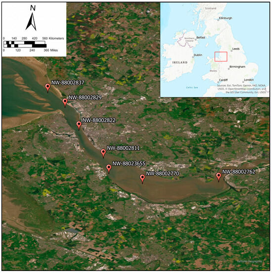
Figure 1.
Map showing the location of the River Mersey Estuary in Northwest England.
The River Mersey estuary is recognized as one of the UK’s most altered urban estuaries, with a long history of industrialization, heavy shipping traffic, and associated pollution inputs [22,23]. Through the 19th and 20th centuries, untreated industrial and municipal wastewater discharged into the estuary led to severe degradation, making it one of Europe’s most polluted rivers by the mid-20th century [24]. Significant improvements in water quality have occurred since the 1980s through regulatory interventions, such as the UK Urban Wastewater Treatment Directive and targeted clean-up programs [25,26]. Nevertheless, the Liverpool reach remains vulnerable to sediment resuspension events from dredging, tidal turbine installation, harbor deepening, and vessel movements, all of which influence turbidity dynamics [20,27].
Ecologically, the Mersey estuary presents diverse habitats-foraging and roosting areas for migratory and overwintering birds such as oystercatchers, redshanks, and knot (Calidris canutus), intertidal mudflats, salt marshes and sandbanks [28,29]. The area also supports the benthic invertebrate fauna and turbid estuary fish species [30] and has helped to secure Site of Special Scientific Interest (SSSI) designation for parts of the estuary and Special Protection Areas (SPA) under UK and EU conservation designations [29].
The socio-economic status of this section is significant because the Port of Liverpool is the UK’s busiest and largest deep-water port and an important center for containerized trade, passenger ferry services, and bulk cargo [31]. The estuary is also of considerable interest in relation to renewable energy, with the local offshore wind farms and tidal energy schemes planned in the area [21,32]. This combination of industrial, ecological, and policy relevance positions Liverpool cause the lower reaches of the River Mersey to become a priority area for environmental surveillance.
For this study, in situ observations were collected from seven UK Environment Agency monitoring stations distributed across the lower Mersey from January 2023 to January 2025 (Figure 1). The Environment Agency dataset provides measurements of turbidity in Formazin Turbidity Units (FTU) that have been reported between 23.6 and 598.5 (FTU) over study timeline. Higher turbidity values generally recorded during the winter due to increased river flow and stormwater runoff. These stations also measure relevant water quality parameters such as Water Depth (m), Salinity (ppt), Temperature (°C), and Tide Time (hh.mm), which are considered as reliable ground truth for calibrating and validating satellite and machine learning predictions [13,16]. The total number of in situ measurements collected across all stations and periods amounted to 191 samples, the distribution of samples per station and year is detailed in Table 1.

Table 1.
Distribution of in situ Turbidity Samples per Station and Year.
Considering its hydrodynamic complexity, pollution history, ecological importance, and economic significance, the Liverpool reach of the River Mersey is an ideal case site for the integration of remote sensing, In situ monitoring, and computational modelling towards maximizing turbidity prediction for sustainable estuary management.
2.2. Data Collection
2.2.1. Satellite Imagery and in Situ Match-Ups
For this research, Harmonised Sentinel-2 MSI: MultiSpectral Instrument, Level-2A (SR) imagery was used. This product provides surface reflectance (SR) values which atmospheric correction (AC) have been achieved through the use of the Sen2Cor processor [5,6].
The Sen2Cor processor was selected because it provides the official Level-2A atmospheric correction for Sentinel-2 data, ensuring standardized and radiometrically consistent reflectance products across all acquisition dates [33]. Sen2Cor performs pixel-level correction for molecular scattering, water vapor absorption, and aerosol optical thickness using radiative transfer algorithms optimized for Sentinel-2’s spectral configuration [33]. This makes it particularly suitable for multi-temporal analyses and machine-learning applications requiring consistent surface reflectance retrievals. Although alternative correction models such as 6S [34] or QUAC [35] can perform well in optically complex or aerosol-rich coastal waters, they rely on ancillary atmospheric inputs (e.g., AERONET aerosol profiles or in situ optical depth measurements) that were unavailable for the River Mersey during this study. While Mersey’s industrial surroundings may elevate aerosol loading, sensitivity checks on corrected reflectance spectra indicated stable Sen2Cor performance, consistent with previous evaluations in similar turbid estuarine settings [36]. Minor residual uncertainties associated with complex aerosol composition are acknowledged in the Discussion as a potential source of reflectance variability.
Sentinel-2 images are characterized by their spatial resolution (10m, 20m, and 60m bands) and the high frequency of revisit (5 days near the equator with two satellites), which makes them especially well-suited to monitoring dynamic aquatic ecosystems [7]. By converting Top-Of-Atmosphere (TOA) reflectance or radiance to Bottom-Of-Atmosphere (BOA) surface reflectance, it ensures that pixel values are indeed representing the true reflectance properties of the Earth’s surface and may be applied directly in quantitative analysis like index computation [15,37]. For this research, the Sentinel Application Platform (SNAP) was selected to perform the pre-processing stage.
Due to frequent cloud cover and Sentinel-2’s revisit schedule, a ±3-day satellite–in situ matchup window was adopted as a practical compromise to secure adequate matched samples; this choice was validated with a targeted sensitivity analysis (0, ±1, ±2, ±3 days) whose diagnostics are provided in Table S2. When cloud-free Sentinel-2 images were available on the exact sampling date, they were prioritized; however, restricting the analysis to same-day or ±1-day pairs would have produced too few valid matchups for reliable model development. Applying the ±3-day window increased the number of valid satellites–in situ pairs to 83 out of 191 total observations, ensuring adequate temporal and spatial representation while maintaining data quality. Comparable short multi-day windows (3–10 days) have been successfully applied in water-quality and hydrological remote-sensing studies to balance matchup density and predictive accuracy [38,39,40,41]. To minimize temporal mismatch, all selected satellite scenes corresponded to comparable tidal stages and non-dredging periods verified through Environment Agency records. Furthermore, tide-related variables (water depth and tide time) were later incorporated as auxiliary predictors to account for short-term hydrodynamic variability associated with tidal forcing.
Additional filtering criteria were applied to ensure matchup reliability. Sentinel-2 scenes with cloud coverage greater than 40% were excluded [42]. Likewise, in situ turbidity values exceeding 400 FTU were removed because, at very high concentrations, optical saturation limits the satellite’s ability to distinguish true reflectance signals [7]. This selection of filtering criteria is a widely adopted practice in remote sensing to ensure the quality and consistency of matchup data. This action minimizes the impact of temporal variability and atmospheric interference [5,7,42].
Out of the 191 in situ measurements collected between January 2023 and January 2025 (see Table 1), this filtering process yielded a total of 83 matched Sentinel-2 image pairs, which were used for spectral-index extraction and preparation of the fused dataset for machine-learning analysis.
2.2.2. Water Parameters
Coastal and estuarine environments, such as the Mersey environment, have more complex dynamics than lakes [18,20], which result in turbidity being more difficult to retrieve as a single parameter [23]. In this study, four water quality parameters include Water Depth (m), Salinity (ppt), Temperature (°C), and Tide Time (hh.mm) were selected from all parameters reported by the UK Environment Agency (see Figure 1), due to their direct effect on turbidity values. Their inclusion improves the accuracy of satellite-based turbidity estimates when integrated into machine learning algorithms. Descriptive statistics (minimum, maximum, and median values) for these parameters at each monitoring station are provided in Table 2. The significance of each parameter for turbidity retrieval is outlined as follows:
Table 2.
Summary statistics (minimum, maximum, and median) of water parameters used in turbidity modelling for the River Mersey estuary.
- Tide Time (hh.mm): Tides are the main reason for water and sediment transport in coastal areas. This is evident when tidal cycles can produce high turbidity values during an ebb or flood tide due to the increased water velocity and consequent resuspension of bed sediments [43]. This is perhaps the most important parameter for the River Mersey estuary, which has one of the largest tidal ranges in the world [44]. The cyclical, dynamic nature of tidal cycles is an important temporal input to any model looking to make reliable turbidity predictions because it includes prominent, predictable resuspension events that are normally elusive to observation through a satellite alone.
- Water Depth (m): Shallow areas experience higher sediment resuspension due to wave action and boat traffic, which increases turbidity [45]. The River Mersey estuary is characterized by extensive intertidal mudflats and a highly variable depth profile, which emphasizes the importance of this parameter. Water depth considerations in the model help to distinguish between naturally turbid shallow regions and deeper areas, providing useful background to the satellite observation [43,46].
- Salinity (ppt): Salinity gradients indicate the mixing of freshwater from the river and saltwater from the sea and are typical of estuarine environments [27]. These interactions have implications regarding the flocculation of suspended particulate material, or the clumping together of small particles into larger aggregates that settle more easily [21]. Flocculation is especially relevant to the River Mersey estuary due to the strong tidally induced mixing in the estuary [21,43]. The model will assimilate salinity measurements to compensate for these variations in particle dynamics, which are directly measurable in turbidity.
- Temperature (°C): Water temperature acts as a dominant driver of water density and stratification, which then drives vertical mixing and sediment resuspension [21,47]. There is considerable seasonal temperature variability in the River Mersey, which influences water density (and biological activity), including phytoplankton growth, which is another contributor to turbidity [48,49]. By incorporating the temperature item, the model will consider seasonal and thermal properties of suspended matter composition and concentration.
3. Methodology
This study involved collecting remote sensing data from Sentinel-2 and in situ measurements to create a reliable machine learning model to enhance turbidity predictions of the River Mersey estuary. The process involves several key steps: a water masking procedure to isolate the area of interest, the calculation of spectral indices from satellite imagery to monitor turbidity level, the application of machine learning algorithms to establish a predictive relationship, and the validation of the model’s performance. The final output from the machine learning validated model will determine improvement level of forecasting, which can be the starting point for deciding satellite data alone are able to generate sufficient results or there is a need for involving a Computational Fluid Dynamics (CFD) model in addition to the in situ measurements to validate Machine Learning model for the turbidity tracking. The detailed process is discussed in Figure 2.
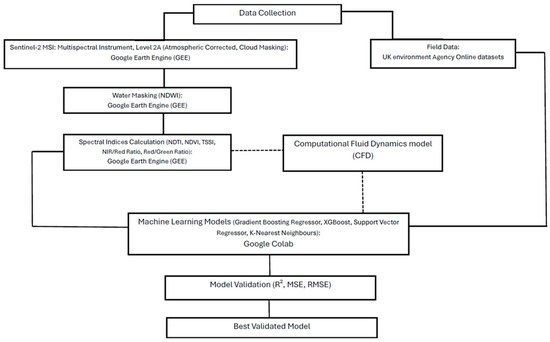
Figure 2.
Flowchart of the methodology.
3.1. Google Earth Engine (GEE)
The methodology involved using Google Earth Engine (GEE) for data processing and downloading Imagery from January 2023 to January 2025, using cloud filters (<40%) and clipping to the lower reach of River Mersey region within the ±3-day window of each in situ measurement [7,41,50]. Noise and cloud interference are minimized by creating a median composite for each match-up dataset. GEE is an online, freely available, cloud-based geospatial processing platform with access to a petabyte-scale catalogue of satellite imagery and geospatial datasets, providing massive computational resources for the analysis of the entire planet [51,52]. The platform offers efficient access to data, pre-processing, and calculating spectral indices of the study area. The Python v.3.13.9 or JavaScript v.2025 programming languages are needed in order to use these datasets and conduct analyses. In this research, JavaScript was selected as a programming language to generate various turbidity indices.
3.2. Water Mask (NDWI)
To isolate water pixels from land and other non-water features, the Normalised Difference Water Index (NDWI) is used as a water mask method. This is a common method for creating a water mask, which leverages the spectral differences between water and land. Water bodies typically absorb light in the near-infrared (NIR) and short-wave infrared (SWIR) bands while reflecting it in the green band, whereas land and vegetation reflect strongly in the NIR [53]. The NDWI applied to Sentinel-2 images, which were filtered by a ±3-day window of field sampling, clipped based on the study area and 40% cloud masking in the Google Earth Engine using the following formula:
where
NDWI = (Green − NIR)/(Green + NIR)
- Green refers to the reflectance in the green band.
- NIR refers to the reflectance in the Near-Infrared band.
The final images are categorized as binary images where 1 represents water pixels and 0 represents non-water pixels. This step ensures that subsequent turbidity retrievals are not contaminated by mixed or non-water pixels.
3.3. Indices Used for Turbidity Monitoring with GEE
For each matched dataset from the Sentinel-2 imagery, six spectral indices (NDTI, NDVI, TSSI, NIR/Red Ratio, Red/Green Ratio) were applied. These indices were selected based on their sensitivity to water quality parameters, particularly turbidity and suspended sediment concentrations, as recommended in other remote sensing research. Table 3 provides a summary of these indices.
Table 3.
Summary of spectral indices derived from Sentinel-2 imagery for turbidity modelling.
3.4. Machine Learning Models
The core objective of this study is to establish a robust and predictive relationship between the satellite-derived spectral indices and the corresponding in situ turbidity measurements. As was mentioned, non-linear correlations between multi-band imagery and in situ turbidity measurements can be evaluated through the application of machine learning algorithms [16,57]. This approach allows for the retrieval of turbidity values over the entire study area, expanding beyond the limited point-source data from field sampling.
3.4.1. Data Preprocessing
After the collection and alignment of in situ and satellite data, a number of strict preprocessing procedures were followed to condition the fused dataset for machine learning model building. Such preprocessing was necessary to ensure quality, continuity, and appropriateness of the data to the selected algorithms, thus improving model accuracy and reliability. The combined dataset was initially loaded into the analytical environment with 83 matched samples that contain both in situ measurements and derived spectral indices.
In addition, missing values (NaNs) were resolved. Any rows with null values in the target variable (Turbidity) or any of the specified input features (spectral indices, Water Depth, Salinity, Temperature, Tide Time) were removed systematically from the dataset. This helped ensure that all samples utilized during model training and assessment were complete and sound.
During data cleaning, turbidity measurements exceeding 400 FTU were excluded. This threshold reflects the optical saturation limit of Sentinel-2 MSI in highly turbid estuarine waters, where water-leaving reflectance signals become non-linear and unreliable for quantitative retrievals [58,59]. Similar upper thresholds are commonly applied in remote-sensing studies of coastal and estuarine waters to avoid radiometric distortion under extreme sediment concentrations [60,61]. Although these high-turbidity events, often triggered by storms, dredging, or resuspension, are ecologically important, their transient nature and the optical limitations of Sentinel-2 (e.g., saturation of red bands beyond 250 FNU) reduce their suitability for quantitative model calibration using multispectral imagery with a five-day revisit cycle [46]. Thus, excluding these outliers ensured model robustness and numerical stability, while acknowledging that capturing extreme-event dynamics remains a promising avenue for future research combining machine learning with hydrodynamic modeling approaches.
A very important step in preparing the environmental dataset was outlier removal [62]. The Interquartile Range (IQR) method was applied to identify and mitigate the influence of extreme data points within the Turbidity (FTU) and the other environmental parameters (excluding Latitude and Longitude, as their ‘outliers’ typically represent incorrect measurements rather than statistical extremes in distribution) [62,63]. A form of outliers as values that lie below:
Or above:
where
- Q1 = First quartiles
- Q3 = Third quartiles, respectively, and
- IQR = The interquartile range (Q3−Q1).
A per-variable interquartile-range (IQR) audit was applied independently to turbidity, six spectral indices (NDTI, NDVI, TSSI, NIR/Red, Red/Green, NDWI), and four auxiliary parameters (water depth, salinity, temperature, tide time). For each variable we computed Q1 and Q3 and flagged values outside. A row-level audit was produced such that any observation flagged in one or more variables was removed from the training dataset. Applying this audit reduced the matched dataset from N = 83 to N = 57 samples. The counts of unique rows flagged per variable are provided in Table 4. The complete row-level audit is provided as Table S1 (outlier_audit_log.csv).
Table 4.
The number of outliers removed per variable.
Upper-range turbidity measurements (160 FTU) identified by the IQR method but retained in the final dataset were verified as genuine environmental signals. These values coincided with high-tide conditions and were consistent with turbidity magnitudes reported in other tide-dominated estuaries globally, for example, suspended sediment concentrations exceeding 1 g·L−1 observed along the Amazon coast [64] and FTU values above 150 recorded in the Cam–Nam Trieu Estuary, Vietnam [65]. Such comparisons confirm that the retained high-turbidity data represent real short-term environmental variability rather than measurement anomalies.
Following this, using the method of IQR, the initially 83 matched samples dataset was narrowed down to 57 clean outlier-free samples to ensure a strong basis for model development.
The pre-processed dataset was separated for model training and evaluation purposes. One train-test split was performed for preliminary exploration and for thorough error analysis, using 80% of the dataset for training purposes and the remaining 20% for testing purposes [66]. There are about 45 samples for training and 12 samples for testing, using a random state of 42 for reproducibility of the split.
To achieve a stronger and less biased evaluation of model performance, particularly due to the small dataset size, 5-fold cross-validation was also utilized. This method divides the dataset into five equal parts randomly. The model was trained on four subsets and validated on the remaining subsets, with this procedure repeated five times to ensure that each subset acted as the validation set once [63]. Spatial robustness was further evaluated using leave-one-station-out (LOSO) cross-validation, in which each monitoring station was held out once as an independent test set to quantify spatial generalization across sites.
3.4.2. Model Selection
Identifying the top-performing algorithm that can effectively capture the relationship between the satellite-derived spectral indices, in situ environmental factors, and the measured turbidity (FTU) values was the main objective of developing a machine learning workflow. Four models were selected to examine different learning paradigms and their suitability for the complex; non-linear relationships found in environmental data [57,67]. The entire machine learning workflow, including data manipulation, model implementation, and evaluation, was conducted using Google Colab platform. The machine learning algorithms examined and implemented herein were:
- Gradient Boosting Regressor (GBR): GBR is an ensemble learning method that sequentially adds multiple weak decision trees to generate a strong predictive model [67,68].
- XGBoost Regressor: XGBoost (eXtreme Gradient Boosting) is a very optimized and efficient implementation of gradient boosting. It is well known for its speed, performance, and adaptability and includes improvements like parallel processing, management of missing variables, and regularization to avoid overfitting [57,69].
- Support Vector Regressor (SVR): SVR can be set up to handle non-linear relationships through the use of kernel functions (Radial Basis Function (RBF) kernel utilized in this study), and is also insensitive to outliers, making it a well-liked choice in water quality parameter retrieval from remote sensing [57,67].
- K-Nearest Neighbors (KNN) Regressor: KNN is a non-parametric, instance-based algorithm that predicts the value of a new instance to be the average of the target values of its ‘k’ Nearest Neighbors in the feature space. Its interpretability and ability to model local trends without making any assumptions about data distribution make it a valuable baseline to compare against in most environmental modelling [57,70]. For this research, a value of 5 for neighbors were utilized.
Every model was trained using the scaled training data (80% of the filtered data) and then tested on the unseen test set (20% of the filtered data) to determine its ability to generalize [66]. While default hyperparameters for every model were used initially, the inherent robustness of ensemble models like GBR and XGBoost, together with feature scaling for SVR and KNN, was designed to provide competitive baseline performance.
The use of 5-fold cross-validation, as described in Section 3.4.1 was at the core of the model training and evaluation. This technique provided a more reliable and less biased estimate of each model’s performance by averaging metrics across multiple train-test splits, thereby mitigating the impact of random data partitioning, overfitting and offering insight into model stability given the dataset’s size [63,71].
3.5. Validation and Accuracy Assessment
To comprehensively assess the predictive performance and accuracy of the trained machine learning models in predicting turbidity, a set of quantitative assessment metrics was employed [67,72,73]. The metrics provide an entire description of how well each model generalizes new data and the magnitude of its prediction errors. The evaluation was performed for the individual train-test split as well as, more importantly, averaged over the 5-fold cross-validation to ensure robust and unbiased performance estimates [73]. These metrics are defined as:
Coefficient of Determination ():
Mean Squared Error (MSE):
Root Mean Squared Error (RMSE):
Mean Absolute Error (MAE):
where
- n = The number of points
- = The actual value,
- = The predicted value
- = The Mean of the actual values
4. Results
This section presents the performance of the machine learning model and key results. These models were trained to predict water turbidity using a combination of remote sensing data and in situ measurements. The per-parameter IQR audit flagged 26 unique observations and yielded a final, outlier-free dataset of 57 samples for model training. Turbidity values exceeding 400 FTU were not retained in the final dataset (no retained samples >400 FTU after filtering). The row-level audit (Table S1) lists each removed observation, the variables that triggered the flag(s), and the removal reason.
4.1. Model Performance and Validation
The predictive capability of four machine learning models, Gradient Boosting Regressor (GBR), XGBoost, Support Vector Regressor (SVR), and K-Nearest Neighbours (KNN) Regressor, was evaluated with the assistance of a K-Fold cross-validation technique. Among the tested algorithms, the best performing was the Gradient Boosting Regressor (GBR) (R2 = 0.84, RMSE = 15.03 = FTU, and MAE = 10.38 FTU). This confirms the suitability of ensemble tree-based approaches for supporting the non-linear and multi-factorial dynamics of turbidity in estuarine environments. Table 5 summarizes the performance of each model.
Table 5.
Model performance metrics for single train-test split.
To further minimize bias due to the relatively small size of the dataset, 5-fold cross-validation was used with mean results presented in Table 6. Cross-validation indicated marginally lower R2 values for all models; however, GBR again reported the best performance (average R2 = 0.54), followed by XGBoost (R2 = 0.54), SVR (R2 = 0.42) and KNN (R2 = 0.21), respectively. The marginally lower R2 values during cross-validation support the sensitivity of turbidity modelling in estuaries to sampling error and the importance of rigorous validation.
Table 6.
Cross-validation results (5-fold) for machine learning models.
The scatterplots observed vs. predicted turbidity scatterplots (Figure 3) provide further insight into model performance. GBR and XGBoost are closer to the 1:1 line than SVR and KNN, more scattered and with systematic underestimation for higher turbidity (>120 FTU). The limited performance of KNN likely reflects its sensitivity to sparse sampling in multi-dimensional feature space, which is typical for environmental datasets of modest size.
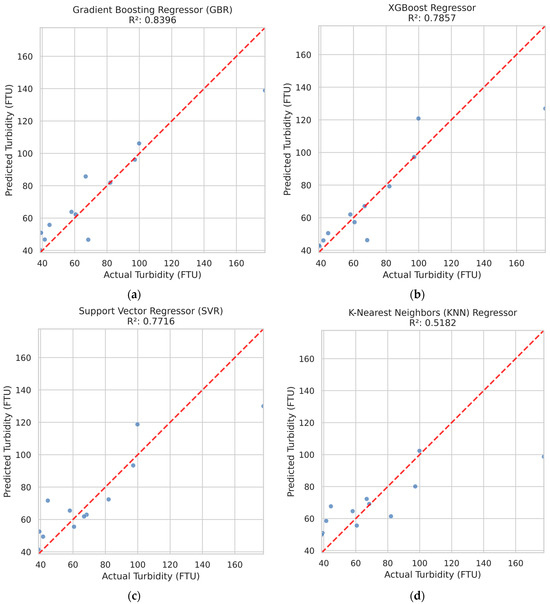
Figure 3.
Scatterplots observed vs. predicted turbidity for (a) Gradient Boosting Regressor; (b) XGBoost Regressor; (c) Support Vector Regressor; (d) K-Nearest Neighbors (KNN) Regressor. The dashed 1:1 line indicates perfect agreement between observed and predicted values.
The turbidity and explanatory variables histograms (Figure 4) illustrate the skewness of the dataset. The most turbidity measurements fall in the range 20–60 FTU, but with some extreme instances up to 160 FTU. While not common, these outliers are environmentally significant and represent high-flow or tidal events in shallow waters. To minimize their effect, the Inter-quartile Range (IQR) method was employed during preprocessing, allowing robust model training.
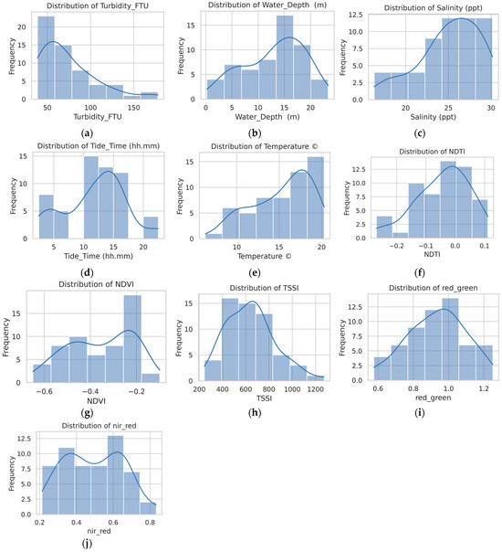
Figure 4.
Histograms and kernel density distributions of the turbidity (FTU) and explanatory variables used in model development: (a) Turbidity; (b) Water Depth; (c) Salinity; (d) Tide Time; (e) Temperature; (f) NDTI; (g) NDVI; (h) TSSI; (i) red/green ratio; and (j) NIR/red ratio. These distributions illustrate the variability and spread of the dataset, providing insights into data balance, potential skewness, and suitability for machine learning modeling.
Residual analysis also highlights the reasons for prediction error (Figure 5). Outliers such as the 160 FTU case under-predicted at 120 FTU were often associated with shallow water, high tidal currents, or stratification due to salinity gradients. Such conditions create sharp localized turbidity spikes that may not be fully captured at satellite overpass times. These findings emphasize the necessity to consider temporal mismatches between in situ and remote sensing observations, as well as the effect of unobserved physical processes such as bottom sediment type, current direction, and wind-driven resuspension.
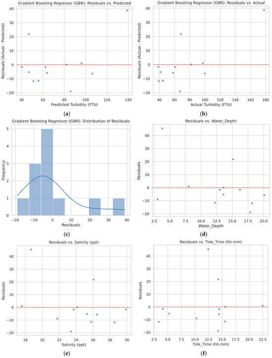
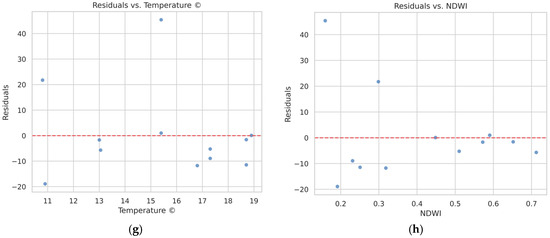
Figure 5.
Diagnostic plots of the Gradient Boosting Regressor (GBR) model. (a) Residuals vs. Predicted turbidity values; (b) Residuals vs. Actual turbidity values; (c) Distribution of Residuals. These plots confirm the model’s residuals are randomly distributed around zero, indicating no systematic errors. (d) Residuals vs. Water Depth; (e) Residuals vs. Salinity; (f) Residuals vs. Tide Time; (g) Residuals vs. Water Temperature; and (h) Residuals vs. NDWI. These plots examine the model’s performance against key features, showing no strong trends and affirming the model’s robust predictive capability across different variables.
To further assess the temporal robustness of the Gradient Boosting Regressor (GBR), a post hoc seasonal evaluation was performed by dividing the dataset into summer–autumn and winter–spring subsets. The model achieved R2 = 0.67 for summer–autumn and R2 = 0.57 for winter–spring. The modest difference between these seasonal values indicates that the GBR model maintained consistent predictive capability across contrasting hydrodynamic and optical regimes, demonstrating satisfactory temporal stability within the River Mersey estuary despite limited sample size and strong environmental variability.
The LOSO evaluation yielded station-wise R2 values from 0.03 to 0.65 (median = −0.35), with model accuracy decreasing whenever a station was excluded (ΔR2 < 0). Excluding any individual station consistently reduced model performance, confirming that each site contributes meaningful variability to the regression. The largest sensitivity occurred for stations NW-88002829, NW-88002837, and NW-88002811 (ΔR2 ≈ −0.6 to −0.8), which capture the dominant spatial gradients of turbidity within the estuary. These results clarify that the observed decline between train–test and cross-validation performance primarily reflects spatial heterogeneity rather than model overfitting. A full summary of the station-specific influence is provided in Table S3, and LOSO scatter plot are included as Figure S5.
4.2. Spatiotemporal Turbidity Analysis
4.2.1. Two-Dimensional Turbidity Maps
Two-dimensional maps were plotted for all four of the machine learning models, Gradient Boosting Regressor (GBR), XGBoost, Support Vector Regressor (SVR), and K-Nearest Neighbours (KNN), to visually assess their predictive performance across the study area. This approach provides the optimal way to identify which model not only performed optimally statistically (see Table 4) but also most effectively captured the spatial patterns of turbidity in the Mersey Estuary.
These maps, as shown in Figure 6, offer a critical means of visually confirming the predicted outcomes. The maps for each model contain three significant layers: actual turbidity, predicted turbidity, and the residuals of the prediction (actual vs. predicted difference). The direct visual comparison of the predicted maps for each model reveals apparent differences.
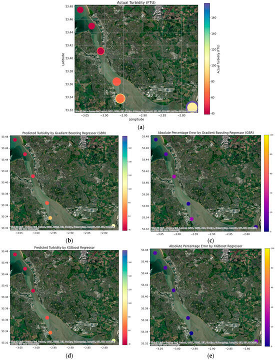
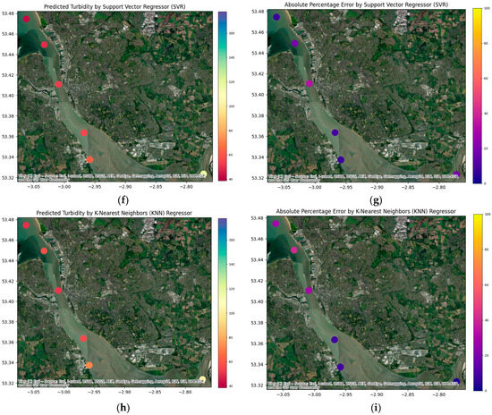
Figure 6.
Two-dimensional spatial maps of turbidity comparing four machine learning models. (a) shows the actual measured turbidity values. The predicted turbidity values are shown for (b) GBR, (d) XGBoost, (f) SVR, and (h) KNN. The corresponding prediction residuals (Actual-Predicted) are shown for (c) GBR, (e) XGBoost, (g) SVR, and (i) KNN. This figure provides a visual comparison of how each model performs in spatially predicting turbidity and highlights the areas of the largest prediction errors.
The GBR predicted map has the closest fit to the actual turbidity mapping patterns (Figure 6b) between the actual turbidity map with the lowest and most uniform residuals. In comparison, the SVR and KNN models both accounted for a greater proportion of spatial data excluded from the residual data in the high turbidity areas, suggesting that these models do not adequately account for some of the non-linear and spatial relationships, as demonstrated by the three-calibrated models. The XGBoost model plotted similarly to the GBR but with slightly higher residual values in certain areas (Figure 6e). As shown in Table 4 and complemented with statistical testing, the model comparisons and performance gathered from all three models provide evidence to support GBR as the model with the best fit to observe data in this study.
4.2.2. Three-Dimensional Turbidity Maps
In this study, three-dimensional scatter plots were generated from the GBR model to produce a more informative and detailed understanding of the turbidity distribution. These plots are particularly suitable for visualizing the complex relationships between turbidity and multiple spatial parameters. As shown in Figure 7, one set of plots visualizes turbidity as a function of longitude and latitude. The size and color of the data points charted in the plot relate to the value of turbidity, offering a better 3D perception of high and low turbidity.
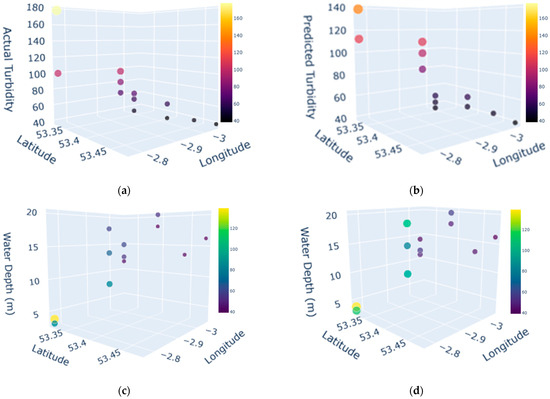
Figure 7.
Three-dimensional plots of turbidity and water depth (a) actual turbidity (FTU) at stations (b) predicted turbidity (FTU) by GBR at stations (3D) (c) actual turbidity (FTU) vs. water depth (m) at stations (d) predicted turbidity (FTU) vs. water depth (m) at stations.
A further set of 3D plots, which are presented in Figure 7, integrates water depth as the vertical axis. This type of visualization is crucial to examine the relationship between turbidity and bathymetry. The values change in turbidity when it is considered as a function of water depth, which indicates how the physical dynamics of the water columns, such as tidal currents or stratification, can influence the distribution of suspended sediment. The interactive nature of these plots allows for a dynamic exploration of the data that would be difficult to obtain from static 2D representations.
4.2.3. Limitations and Future Work
The study presents a robust method for turbidity prediction in estuaries from Sentinel-2 images, in situ observations, and machine learning. While the results are promising and demonstrate that satellite-based turbidity estimation is viable, there are areas where possibilities of improvement exist.
First, although the dataset that was used to train the models (n = 57) was prefiltered for quality and consistency, the comparatively small sample size is a common risk in remote sensing applications within estuaries with changing conditions. This final dataset represents roughly 30% of the initially matched records (83 pairs) after outlier auditing, with about 12% of turbidity observations (>400 FTU) excluded because Sentinel-2 MSI red/NIR bands approach optical saturation at such concentrations. Most of the excluded values correspond to short-lived, high-energy events (e.g., storm-driven resuspension or dredging), meaning the resulting model best represents routine turbidity (<400 FTU) rather than extreme conditions. Nevertheless, enforcing rigorous preprocessing steps such as removal of outliers and the use of k-fold cross-validation ensured model stability despite the small sample size. Future research will try to increase the time base and include additional matchups to enable more generalization of the model.
Second, even though the Gradient Boosting Regressor (GBR) had satisfactory predictive capacity (R2 = 0.84 in test and R2 = 0.54 in cross-validation), there were some inconsistencies in turbid areas or in areas where physical processes such as tidal mixing, resuspension, or salinity-driven stratification dominate. These findings are in agreement with previous work that has reported the inadequacy of data-driven models under estuarine conditions where physical forcing is both spatially and temporally heterogeneous [46,67,74].
Third, while this study does not implement CFD modeling, the ability of machine learning to generate spatially complete turbidity maps presents valuable input for future CFD-based analyses. Prior work has shown that using ML-derived inputs can improve initialization and boundary conditions in hydrodynamic simulations [75,76,77]. Given the complex dynamics of the River Mersey, future research could build upon this study’s outputs to develop CFD–ML frameworks for simulating sediment transport and tidal variability.
As shown in the recent literature, coupling ML with CFD enables simulation of time-dependent physical processes, such as sediment transport and tidal circulation, that are difficult to capture with satellite imagery alone [75,76]. Although this integration remains outside the scope of the present work, it represents a viable pathway toward real-time estuarine monitoring, pollution tracking, and improved management of meso-tidal systems. The framework as described, if applied, holds substantial potential to allow for real-time environmental monitoring, pollution tracking, and adaptive estuarine management.
5. Discussion
The main aim of this research was to determine the performance of machine learning models for predicting turbidity in the River Mersey estuary using a limited yet high-quality dataset, reflecting the real-world challenges of estuarine monitoring in persistently cloudy, tidally dynamic environments. The Gradient Boosting Regressor (GBR) model continuously outperformed the other algorithms. It had a cross-validated R2 value of 0.54 and a value of 0.84 in train-test evaluation. This shows that spectral indices from Sentinel-2 imagery can estimate turbidity values across a large area. This finding aligns with previous research supporting the use of machine learning for water quality prediction in aquatic environments [57,66,67,71,78].
The performance differences among the models offer insights into the nature of turbidity dynamics in the estuary. GBR’s superior performance suggests that turbidity variation is driven by complex, non-linear, and interacting processes (e.g., the interplay of tidal stage, water depth, and salinity) that are well-captured by ensemble tree-based models. In contrast, SVR’s assumption of global smoothness and KNN’s locality-based structure were less suited to these heterogeneous dynamics. Thus, GBR’s success reinforces its suitability for modeling such estuarine systems. The success of GBR therefore confirms that ensemble tree-based methods are particularly well-suited to capturing the interacting and highly dynamic drivers of turbidity in estuarine systems.
However, the analysis of the model’s residuals revealed significant limitations, particularly in the highly dynamic mouth of the estuary. The model’s performance was notably weaker in areas dominated by strong tidal currents and advective transport. These results highlight a key limitation of data-driven models [67,74]. While they are able to effectively identify correlations within a dataset, they do not inherently account for the underlying physical principles governing a system. The majority of the errors were probably due to the temporal mismatch between static satellite image acquisition and the rapid, physically driven changes in turbidity caused by tidal cycles and cloud coverage.
This behavior underscores the fundamental distinction between data-driven and physically based models. While the GBR identifies empirical relationships among optical and environmental variables, it cannot explicitly represent the physical mechanisms—such as tidal shear-induced sediment resuspension or salinity-driven flocculation—that govern short-term turbidity fluctuations. In light of this, the current model should be regarded as a diagnostic framework for identifying spatiotemporal turbidity patterns rather than as a mechanistic predictor of process dynamics. Nonetheless, the approach establishes a transferable foundation for hybrid integration with process-based hydrodynamic models in future work.
A complementary Post Hoc seasonal evaluation further clarified this performance pattern. When the dataset was divided into summer–autumn and winter–spring subsets, the GBR achieved R2 values of 0.67 and 0.57, respectively. The small difference between these results indicates that the model maintained a relatively stable predictive skill across distinct hydrodynamic regimes, though minor seasonal fluctuations likely reflect differences in tidal energy, river inflows, and sediment resuspension intensity. These findings suggest that temporal variability, rather than model instability, primarily accounts for the decline observed between train–test and cross-validation metrics. Comparable seasonal sensitivities have been reported in estuarine ML-based water-quality models [64,71,79], where R2 reductions of approximately 0.1–0.3 are common when models are applied across different hydrological or seasonal contexts. The combined seasonal and LOSO analyses indicate that temporal variability and spatial heterogeneity jointly constrain model generalization, consistent with findings from other optically complex estuaries.
Another potential contributor to model uncertainty arises from the atmospheric correction stage. Although the Sen2Cor processor delivers standardized Level-2A surface reflectance products and has been validated for general aquatic applications, it is not specifically optimized for highly aerosol-loaded or industrial estuarine settings such as the River Mersey. Complex mixtures of maritime and anthropogenic aerosols, along with humidity and haze, may introduce subtle variations in retrieved red- and NIR-band reflectance. These residual effects are likely minor relative to turbidity-driven signal changes but could partially explain the moderate decline in cross-validated performance (R2 = 0.54). Similar observations have been reported in evaluations of Sen2Cor and alternative schemes such as 6S and QUAC in coastal environments [33,35,80]. Future work could test these or dedicated aquatic processors (e.g., ACOLITE, C2RCC) to quantify sensitivity to aerosol variability in estuarine conditions.
A further limitation arising from the data quality control process concerns the operational range of the final GBR model. The systematic exclusion of turbidity values exceeding 400 FTU, as justified on radiometric grounds in Section 3.4.1 to avoid signal saturation, means that the resulting model is optimized for routine monitoring of turbidity within the typical estuarine range (Turbidity < 400 FTU). We acknowledge that these omitted high-turbidity observations often coincide with ecologically critical events such as storm-induced or dredging-related sediment resuspension. However, the transient nature of such episodes, combined with the optical saturation of Sentinel-2 MSI red and NIR bands and its five-day revisit cycle, limits the sensor’s ability to capture them quantitatively [58]. Consequently, the present model characterizes typical turbidity dynamics rather than peak disturbance events. Future studies targeting these extreme conditions should consider sensors with a higher radiometric dynamic range (e.g., Landsat-8/9 OLI, which includes the coastal blue band) or employ specialized turbid-water atmospheric correction processors such as ACOLITE or C2RCC [61]. Landsat-8, in particular, has shown promise in highly turbid coastal and inland waters due to its shortwave infrared (SWIR) capabilities and broader dynamic range [80,81]. Incorporating these datasets within a hybrid ML–CFD modelling framework could extend predictive capability to short-lived, high-energy events and improve ecological risk assessment.
These limitations suggest the potential value of combining data-driven approaches with physics-based modeling to provide a more holistic understanding of turbidity variability. In particular, recent studies have explored the integration of machine learning outputs with Computational Fluid Dynamics (CFD) models to enhance the spatiotemporal resolution of environmental monitoring system [75,76,77]. In such hybrid frameworks, ML-generated turbidity maps, such as those developed in this study, may serve as high-resolution inputs to CFD simulations, improving the initialization or boundary conditions of hydrodynamic models.
This approach has been shown in the literature to reduce interpolation errors commonly encountered in CFD modeling, which typically relies on sparse field observations for set up [75,82]. The advantage of using ML output from satellite data is that they offer spatially continuous snapshots of water quality conditions, which are otherwise difficult to obtain through traditional field-based methods [74]. When integrated with CFD solvers based on the Navier–Stokes equations, such inputs could enable simulations of turbidity transport in response to tidal cycles, river inflows, and sediment resuspension events.
Although CFD modeling was not implemented in the present study, the demonstrated ability of GBR to capture spatial patterns of turbidity indicates that ML outputs have potential to complement physics-based approaches in future work. This form of hybridization, as described in the recent literature, could improve forecasting capabilities and support real-time estuarine monitoring and management. This study focused on the development and validation of machine learning models using satellite and in situ data, also implementation of CFD simulations was beyond the scope of this study but represents a potential avenue for future investigations. The successful application of the Gradient Boosting Regressor (GBR) in predicting turbidity provides a spatially continuous initial condition that can be used to initialize or enhance 3D hydrodynamic CFD simulations. This hybrid approach aims to bridge the current gap between spatial coverage (from remote sensing) and physical realism (from numerical modeling). Implementation of CFD simulations is planned as part of future work.
Future Research Directions (CFD Integration)
A possible future stage of this research could involve the use of Computational Fluid Dynamics (CFD) to provide a comprehensive dataset where satellites data are limited to enhance machine learning models (Figure 2). These outputs serve as a critical foundation for future work, where they will be integrated into a framework [77]. For the Mersey estuary, this integration is critical, given that it will allow for the simulation of dynamic physical processes such as tidal cycles and currents, where satellite data are limited. However, CFD models are computationally expensive and time consuming [83], their output can be used to fill the temporal and spatial gaps left by satellite data. The successful machine learning model developed in this study serves as a critical foundation for this future work. They may be integrated into a hybrid framework in subsequent studies, where satellite data informs and validates CFD models, and CFD, in turn, provides the critical data where satellite information is limited [78]. This approach is essential for understanding the temporal evolution and transport of turbidity within the coastal environment [75,76]. While this study does not implement CFD modeling, the ability of machine learning to generate spatially complete turbidity maps presents valuable input for future CFD-based analyses. Prior work has shown that using ML-derived inputs can improve initialization and boundary conditions in hydrodynamic simulations [75,76,77]. Given the complex dynamics of the River Mersey, future research could build upon this study’s outputs to develop CFD–ML frameworks for simulating sediment transport and tidal variability.
6. Conclusions
This study demonstrated the viability of the integration of Sentinel-2 imagery with machine learning models for turbidity estimation in the highly dynamic environment of the River Mersey estuary under a limited dataset. The main dataset was a combination of spectral indices and in situ measurements, which generated reliable turbidity maps and highlighted the potential of Earth observation data for coastal monitoring. The methodological framework combined satellite image preprocessing (cloud filtering, atmospheric correction, and spectral index calculation), in situ matchups, and advanced regression models validated with cross-validation. This stepwise approach ensured that both the spatially extensive coverage of remote sensing and the ground-truth accuracy of field measurements were effectively utilized. Moreover, the use of four different algorithms provided a robust comparison, demonstrating the value of ensemble methods in handling non-linear and multi-factor interactions typical of estuarine systems.
The Gradient Boosting Regressor (GBR) model was the best among the four algorithms trialed, having an R2 of 0.54 under cross-validation that makes it robust in explaining non linear relationships between spectral indices, in situ water characteristics, and turbidity [82]. This confirms that ensemble-based approaches offer a solid predictive model for optically complex estuarine waters than simpler versions such as KNN or SVR. Despite such promising findings, analysis still pointed out intrinsic limitations of purely data-driven approaches in estuarine settings.
Despite these strengths, challenges remain in accounting for temporal variability and dynamic hydrodynamic processes, particularly in areas influenced by tidal forces. These limitations suggest opportunities for future research to explore hybrid modeling frameworks that incorporate both data-driven and physics-based techniques. As shown in recent studies, integrating machine learning outputs with hydrodynamic models such as Computational Fluid Dynamics (CFD) may improve the spatiotemporal accuracy of predictions in complex coastal systems. While this integration was not within the scope of the current study, the turbidity maps developed here may support such applications in future investigations.
Overall, this work provides a foundation for advancing satellite-based turbidity monitoring and contributes to the growing body of knowledge supporting the use of machine learning in environmentally remote sensing. Future studies could also extend this methodology to longer time series and other estuaries, making these tools more effective for sustainable coastal management, pollution monitoring, and climate resilience planning in the UK and other regions.
Supplementary Materials
The following supporting information can be downloaded at: https://www.mdpi.com/article/10.3390/rs17213617/s1, Table S1: Outlier Audit Log for the Merged Dataset, Table S2: Matchup Window Sensitivity Results for GBR and Ridge Models, Data S1: Full Model Residuals Data frame, Figure S1: Residuals versus Tide Time for the Global GBR Model, Figure S2: Residuals versus Water Depth for the Global GBR Model, Figure S3: Spatial Distribution of Absolute Residuals across Sampling Stations (Residual Map), Figure S4: Distribution of Model Residuals (Histogram), Table S3: Station-Specific Model Performance Metrics (R2, RMSE, MAE) With and Without the Station in the Training Data (Leave-One-Station-Out Results), Figure S5: Scatter Plot of Measured vs. Predicted Turbidity for the Leave-One-Station-Out (LOSO) Cross-Validation.
Author Contributions
Conceptualization, D.N. and M.A.; methodology, D.N. and M.A.; software, D.N.; validation, D.N., M.A. and I.C.; formal analysis, D.N.; investigation, D.N.; resources, I.C.; data curation, D.N. and M.A.; writing—original draft preparation, D.N.; writing—review and editing, D.N., M.A. and I.C.; visualization, D.N. and I.C.; supervision, M.A. and I.C.; project administration, I.C.; funding acquisition, I.C. All authors have read and agreed to the published version of the manuscript.
Funding
This research received no external funding.
Data Availability Statement
The data used to support the findings of this study are free publicly available. The field data were sourced from the UK Environment Agency Online datasets (https://environment.data.gov.uk/water-quality/view/, accessed on 12 March 2025), and the satellite imagery was obtained from the Sentinel-2 Multispectral Instrument (MSI) via the Google Earth Engine (GEE) platform (https://earthengine.google.com/, accessed on 30 May 2025).
Acknowledgments
During the preparation of this manuscript, the author used ChatGPT version GPT-5 and Grammarly to support language polishing and structuring of sections. The authors have reviewed and edited the output and take full responsibility for the content of this publication.
Conflicts of Interest
The authors declare no conflict of interest.
Abbreviations
The following abbreviations are used in this manuscript:
| Avg | Average (mean value, typically across k-fold cross-validation) |
| BOA | Bottom of Atmosphere |
| CFD | Computational Fluid Dynamics |
| GBR | Gradient Boosting Regressor |
| GEE | Google Earth Engine |
| KNN | K-Nearest Neighbors |
| MAE | Mean Absolute Error |
| MSE | Mean Squared Error |
| NDTI | Normalized Difference Turbidity Index |
| NDVI | Normalized Difference Vegetation Index |
| NDWI | Normalized Difference Water Index |
| R2 | Coefficient of Determination |
| RMSE | Root Mean Squared Error |
| SPA | Special Protection Areas |
| SR | Surface Reflectance |
| SSSI | Site of Special Scientific Interest |
| Std | Standard Deviation (variability measure, typically across k-fold cross-validation) |
| SVR | Support Vector Regressor |
| TOA | Top of Atmosphere |
References
- United Nations World Water Development Report 2023: Partnerships and Cooperation for Water; United Nations: Paris, France, 2023.
- Vörösmarty, C.J.; McIntyre, P.B.; Gessner, M.O.; Dudgeon, D.; Prusevich, A.; Green, P.; Glidden, S.; Bunn, S.E.; Sullivan, C.A.; Liermann, C.R.; et al. Global threats to human water security and river biodiversity. Nature 2010, 467, 555–561. [Google Scholar] [CrossRef] [PubMed]
- Matos, T.; Martins, M.S.; Henriques, R.; Goncalves, L.M. A review of methods and instruments to monitor turbidity and suspended sediment concentration. J. Water Process. Eng. 2024, 64, 105624. [Google Scholar] [CrossRef]
- Bilotta, G.S.; Brazier, R.E. Understanding the influence of suspended solids on water quality and aquatic biota. Water Res. 2008, 42, 2849–2861. [Google Scholar] [CrossRef]
- Page, B.P.; Olmanson, L.G.; Mishra, D.R. A harmonized image processing workflow using Sentinel-2/MSI and Landsat-8/OLI for mapping water clarity in optically variable lake systems. Remote Sens. Environ. 2019, 231, 111284. [Google Scholar] [CrossRef]
- Pahlevan, N.; Chittimalli, S.K.; Balasubramanian, S.V.; Vellucci, V. Sentinel-2/Landsat-8 product consistency and implications for monitoring aquatic systems. Remote Sens. Environ. 2019, 220, 19–29. [Google Scholar] [CrossRef]
- Casal, G.; Hedley, J.D.; Monteys, X.; Harris, P.; Cahalane, C.; McCarthy, T. Satellite-derived bathymetry in optically complex waters using a model inversion approach and Sentinel-2 data. Estuar. Coast. Shelf Sci. 2020, 241, 106814. [Google Scholar] [CrossRef]
- Lizcano-Sandoval, L.; Anastasiou, C.; Montes, E.; Raulerson, G.; Sherwood, E.; Muller-Karger, F.E. Seagrass distribution, areal cover, and changes (1990–2021) in coastal waters off West-Central Florida, USA. Estuar. Coast. Shelf Sci. 2022, 279, 108134. [Google Scholar] [CrossRef]
- Wang, X.; Song, K.; Wen, Z.; Liu, G.; Shang, Y.; Fang, C.; Lyu, L.; Wang, Q. Quantifying Turbidity Variation for Lakes in Daqing of Northeast China Using Landsat Images From 1984 to 2018. IEEE J. Sel. Top. Appl. Earth Obs. Remote Sens. 2021, 14, 8884–8897. [Google Scholar] [CrossRef]
- Zhang, X.; Huang, J.; Chen, J.; Zhao, Y. Remote sensing monitoring of total suspended solids concentration in Jiaozhou Bay based on multi-source data. Ecol. Indic. 2023, 154, 110513. [Google Scholar] [CrossRef]
- Stramski, D.; Reynolds, R.A.; Babin, M.; Kaczmarek, S.; Lewis, M.R.; Röttgers, R.; Sciandra, A.; Stramska, M.; Twardowski, M.S.; Franz, B.A.; et al. Relationships between the surface concentration of particulate organic carbon and optical properties in the eastern South Pacific and eastern Atlantic Oceans. Biogeosciences 2008, 5, 171–201. [Google Scholar] [CrossRef]
- Zhu, Y.; Cao, P.; Liu, S.; Zheng, Y.; Huang, C. Development of a New Method for Turbidity Measurement Using Two NIR Digital Cameras. ACS Omega 2020, 5, 5421–5428. [Google Scholar] [CrossRef]
- Kuhn, C.; De Matos Valerio, A.; Ward, N.; Loken, L.; Sawakuchi, H.O.; Kampel, M.; Richey, J.; Stadler, P.; Crawford, J.; Striegl, R.; et al. Performance of Landsat-8 and Sentinel-2 surface reflectance products for river remote sensing retrievals of chlorophyll-a and turbidity. Remote Sens. Environ. 2019, 224, 104–118. [Google Scholar] [CrossRef]
- Beck, R.; Xu, M.; Zhan, S.; Johansen, R.; Liu, H.; Tong, S.; Yang, B.; Shu, S.; Wu, Q.; Wang, S.; et al. Comparison of satellite reflectance algorithms for estimating turbidity and cyanobacterial concentrations in productive freshwaters using hyperspectral aircraft imagery and dense coincident surface observations. J. Great Lakes Res. 2019, 45, 413–433. [Google Scholar] [CrossRef] [PubMed]
- Li, J.; Xia, C. Drivers of Spatial and Temporal Dynamics in Water Turbidity of China Yangtze River Basin. Water 2023, 15, 1264. [Google Scholar] [CrossRef]
- Yang, Z.; Gong, C.; Lu, Z.; Wu, E.; Huai, H.; Hu, Y.; Li, L.; Dong, L. Combined Retrievals of Turbidity from Sentinel-2A/B and Landsat-8/9 in the Taihu Lake through Machine Learning. Remote Sens. 2023, 15, 4333. [Google Scholar] [CrossRef]
- El-Magd, I.A.; Hillman, P.F. Geomorphological monitoring of a highly dynamic estuary using oblique aerial photographs. Int. J. Digit. Earth 2009, 2, 109–121. [Google Scholar] [CrossRef]
- Hurley, R.R.; Rothwell, J.J.; Woodward, J.C. Metal contamination of bed sediments in the Irwell and Upper Mersey catchments, northwest England: Exploring the legacy of industry and urban growth. J. Soils Sediments 2017, 17, 2648–2665. [Google Scholar] [CrossRef]
- Davies, A.G.; Robins, P.E.; Austin, M.; Walker-Springett, G. Exploring regional coastal sediment pathways using a coupled tide-wave-sediment dynamics model. Cont. Shelf Res. 2023, 253, 104903. [Google Scholar] [CrossRef]
- Ridgway, J.; Bee, E.; Breward, N.; Cave, M.; Chenery, S.; Gowing, C.; Harrison, I.; Hodgkinson, E.; Humphreys, B.; Ingham, M.; et al. British Geological Survey. The Mersey Estuary: Sediment Geochemistry. 2012. Available online: www.bgs.ac.uk/gsni/ (accessed on 29 June 2025).
- Polton, J.A.; Palmer, M.R.; Howarth, M.J. Physical and dynamical oceanography of Liverpool Bay. Ocean Dyn. 2011, 61, 1421–1439. [Google Scholar] [CrossRef]
- Jones, P.D. Water quality and fisheries in the Mersey estuary, England: A historical perspective. Mar. Pollut. Bull. 2006, 53, 144–154. [Google Scholar] [CrossRef]
- Robins, P.E.; Skov, M.W.; Lewis, M.J.; Giménez, L.; Davies, A.G.; Malham, S.K.; Neill, S.P.; McDonald, J.E.; Whitton, T.A.; Jackson, S.E.; et al. Impact of climate change on UK estuaries: A review of past trends and potential projections. Estuar. Coast. Shelf Sci. 2016, 169, 119–135. [Google Scholar] [CrossRef]
- Johnston, P.A.; Stringer, R.L.; French, M.C. Pollution of UK estuaries: Historical and current problems. Sci. Total Environ. 1991, 106, 55–70. [Google Scholar] [CrossRef]
- Hawkins, S.J.; O’Shaughnessy, K.; Adams, L.; Langston, W.; Bray, S.; Allen, J.; Wilkinson, S.; Bohn, K.; Mieszkowska, N.; Firth, L. Recovery of an urbanised estuary: Clean-up, de-industrialisation and restoration of redundant dock-basins in the Mersey. Mar. Pollut. Bull. 2020, 156, 111150. [Google Scholar] [CrossRef]
- Kraberg, A.C.; Wasmund, N.; Vanaverbeke, J.; Schiedek, D.; Wiltshire, K.H.; Mieszkowska, N. Regime shifts in the marine environment: The scientific basis and political context. Mar. Pollut. Bull. 2011, 62, 7–20. [Google Scholar] [CrossRef] [PubMed]
- Essink, K. Ecological effects of dumping of dredged sediments; options for management. J. Coast. Conserv. 1999, 5, 69–80. [Google Scholar] [CrossRef]
- Musgrove, A.; Aebischer, N.; Burnell, D.; Eaton, M.; Frost, T.; Hall, C.; Stroud, D.; Noble, D. Population estimates of birds in Great Britain and the United Kingdom. Br. Birds 2013, 106, 64–100. [Google Scholar]
- Buck, A.L.; Davidson, N.C.; Donaghy, A. An Inventory of UK Estuaries. Vol. 1: Introduction and Methodology; Joint Nature Conservation Committee: Peterborough, UK, 1997. [Google Scholar]
- Langston, W.J.; Chesman, B.S.; Burt, G.R. Site Characterisation of European Marine Sites. The Mersey Estuary SPA; Marine Biological Association of the United Kingdom: Plymouth, UK, 2006. [Google Scholar]
- Wilmsmeier, G.; Monios, J. Counterbalancing peripherality and concentration: An analysis of the UK container port system. Marit. Policy Manag. 2013, 40, 116–132. [Google Scholar] [CrossRef]
- Mclachlan, C. Tidal Stream Energy in the UK: Stakeholder Perceptions Study; University of Manchester: Manchester, UK, 2010. [Google Scholar]
- Main-Knorn, M.; Pflug, B.; Louis, J.; Debaecker, V.; Müller-Wilm, U.; Gascon, F. Sen2Cor for Sentinel-2. In Image and Signal Processing for Remote Sensing XXIII; Bruzzone, L., Bovolo, F., Benediktsson, J.A., Eds.; SPIE: Warsaw, Poland, 2017; p. 3. [Google Scholar] [CrossRef]
- Kotchenova, S.Y.; Vermote, E.F.; Matarrese, R.; Klemm, F., Jr. Validation of a vector version of the 6S radiative transfer code for atmospheric correction of satellite data. Part I: Path radiance. Appl. Opt. 2006, 45, 6762–6774. [Google Scholar] [CrossRef] [PubMed]
- Bernstein, L.S.; Jin, X.; Gregor, B.; Adler-Golden, S.M. Quick atmospheric correction code: Algorithm description and recent upgrades. Opt. Eng. 2012, 51, 111719. [Google Scholar] [CrossRef]
- Vanhellemont, Q.; Ruddick, K. Atmospheric correction of metre-scale optical satellite data for inland and coastal water applications. Remote Sens. Environ. 2018, 216, 586–597. [Google Scholar] [CrossRef]
- Caballero, I.; Stumpf, R.P. Confronting turbidity, the major challenge for satellite-derived coastal bathymetry. Sci. Total Environ. 2023, 870, 161898. [Google Scholar] [CrossRef] [PubMed]
- Lacroix, P.; Bièvre, G.; Pathier, E.; Kniess, U.; Jongmans, D. Use of Sentinel-2 images for the detection of precursory motions before landslide failures. Remote Sens. Environ. 2018, 215, 507–516. [Google Scholar] [CrossRef]
- Liu, Y.; Song, Y.; Liu, P.; Lai, L.; Zhang, Y. Concerns about the temporal matching windows in satellite-ground synchronization for lacustrine environment mapping. Water Res. 2025, 286, 124208. [Google Scholar] [CrossRef]
- Schröder, T.; Schmidt, S.I.; Kutzner, R.D.; Bernert, H.; Stelzer, K.; Friese, K.; Rinke, K. Exploring Spatial Aggregations and Temporal Windows for Water Quality Match-Up Analysis Using Sentinel-2 MSI and Sentinel-3 OLCI Data. Remote Sens. 2024, 16, 2798. [Google Scholar] [CrossRef]
- Kayastha, P.; Dzialowski, A.R.; Stoodley, S.H.; Wagner, K.L.; Mansaray, A.S. Effect of Time Window on Satellite and Ground-Based Data for Estimating Chlorophyll-a in Reservoirs. Remote Sens. 2022, 14, 846. [Google Scholar] [CrossRef]
- Candra, D.S.; Phinn, S.; Scarth, P. Cloud and cloud shadow masking for Sentinel-2 using multitemporal images in global area. Int. J. Remote Sens. 2020, 41, 2877–2904. [Google Scholar] [CrossRef]
- Fischer, A.M.; Pang, D.; Kidd, I.M.; Moreno-Madriñán, M.J. Spatio-Temporal Variability in a Turbid and Dynamic Tidal Estuarine Environment (Tasmania, Australia): An Assessment of MODIS Band 1 Reflectance. ISPRS Int. J. Geo-Inf. 2017, 6, 320. [Google Scholar] [CrossRef]
- Becker, A.; Plater, A.; Wolf, J. The Energy River: Realising Energy Potential from the River Mersey; University of Liverpool and National Oceanography Centre: Liverpool, UK, 2017. [Google Scholar]
- Bu, M.; Li, Y.; Wei, J.; Tang, C. The Influence of Ship Waves on Sediment Resuspension in the Large Shallow Lake Taihu, China. Int. J. Environ. Res. Public Health 2020, 17, 7055. [Google Scholar] [CrossRef] [PubMed]
- Chowdhury, M.; Vilas, C.; van Bergeijk, S.; Navarro, G.; Laiz, I.; Caballero, I. Monitoring turbidity in a highly variable estuary using Sentinel 2-A/B for ecosystem management applications. Front. Mar. Sci. 2023, 10, 1186441. [Google Scholar] [CrossRef]
- Ramírez-Mendoza, R. Flocculation Controls in a Hypertidal Estuary. Ph.D. Thesis, University of Liverpool, Liverpool, UK, 2015. [Google Scholar]
- Shi, M.; Ma, J.; Zhang, K. The Impact of Water Temperature on In-Line Turbidity Detection. Water 2022, 14, 3720. [Google Scholar] [CrossRef]
- Muszel, K. Impact of Sea Surface Temperature and Salinity on Phytoplankton Blooms Phenology in the North Sea. Master’s Thesis, Lund University, Lund, Sweden, 2023. [Google Scholar]
- Bailey, S.W.; Werdell, P.J. A multi-sensor approach for the on-orbit validation of ocean color satellite data products. Remote Sens. Environ. 2006, 102, 12–23. [Google Scholar] [CrossRef]
- Molnár, T.; Király, G. Forest Monitoring Based on Sentinel-2 Satellite Imagery, Google Earth Engine Cloud Computing, and Machine Learning. Preprints 2023. [Google Scholar] [CrossRef]
- Sowrav, S.F.F.; Debsarma, S.K.; Das, M.K.; Ibtehal, K.M.; Rahman, M.; Hridita, N.T.; Broty, A.A.; Hoque, M.S.A. Developing a semi-automated technique of surface water quality analysis using GEE and machine learning: A case study for Sundarbans. Heliyon 2025, 11, e42404. [Google Scholar] [CrossRef]
- McFeeters, S.K. The use of the Normalized Difference Water Index (NDWI) in the delineation of open water features. Int. J. Remote Sens. 1996, 17, 1425–1432. [Google Scholar] [CrossRef]
- Elhag, M.; Gitas, I.; Othman, A.; Bahrawi, J.; Gikas, P. Assessment of Water Quality Parameters Using Temporal Remote Sensing Spectral Reflectance in Arid Environments, Saudi Arabia. Water 2019, 11, 556. [Google Scholar] [CrossRef]
- Helali, J.; Asaadi, S.; Jafarie, T.; Habibi, M.; Salimi, S.; Momenpour, S.E.; Shahmoradi, S.; Hosseini, S.A.; Hessari, B.; Saeidi, V. Drought monitoring and its effects on vegetation and water extent changes using remote sensing data in Urmia Lake watershed, Iran. J. Water Clim. Change 2022, 13, 2107–2128. [Google Scholar] [CrossRef]
- Patil, S.S.; Barfield, B.J.; Wilber, G.G. Turbidity Modeling Based on the Concentration of Total Suspended Solids for Stormwater Runoff from Construction and Development Sites. In Proceedings of the World Environmental and Water Resources Congress 2011, Palm Springs, CA, USA, 22 May 2011; American Society of Civil Engineers: Reston, VA, USA, 2011; pp. 477–486. [Google Scholar] [CrossRef]
- Zhu, M.; Wang, J.; Yang, X.; Zhang, Y.; Zhang, L.; Ren, H.; Wu, B.; Ye, L. A review of the application of machine learning in water quality evaluation. Eco-Environ. Health 2022, 1, 107–116. [Google Scholar] [CrossRef] [PubMed]
- Dogliotti, A.I.; Ruddick, K.G.; Nechad, B.; Doxaran, D.; Knaeps, E. A single algorithm to retrieve turbidity from remotely-sensed data in all coastal and estuarine waters. Remote Sens. Environ. 2015, 156, 157–168. [Google Scholar] [CrossRef]
- Nechad, B.; Ruddick, K.G.; Park, Y. Calibration and validation of a generic multisensor algorithm for mapping of total suspended matter in turbid waters. Remote Sens. Environ. 2010, 114, 854–866. [Google Scholar] [CrossRef]
- Novoa, S.; Doxaran, D.; Ody, A.; Vanhellemont, Q.; Lafon, V.; Lubac, B.; Gernez, P. Atmospheric Corrections and Multi-Conditional Algorithm for Multi-Sensor Remote Sensing of Suspended Particulate Matter in Low-to-High Turbidity Levels Coastal Waters. Remote Sens. 2017, 9, 61. [Google Scholar] [CrossRef]
- Vanhellemont, Q.; Ruddick, K. ACOLITE processing for Sentinel-2 and Landsat-8: Atmospheric correction and aquatic applications. In Proceedings of the Ocean Optics XXIII Conference, Victoria, BC, Canada, 23–28 October 2016; Available online: https://odnature.naturalsciences.be/downloads/publications/oceanoptics2016quinten.pdf (accessed on 7 October 2025).
- Robinson, R.B.; Cox, C.D.; Odom, K. Identifying Outliers in Correlated Water Quality Data. J. Environ. Eng. 2005, 131, 651–657. [Google Scholar] [CrossRef]
- Paepae, T.; Bokoro, P.N.; Kyamakya, K. A Virtual Sensing Concept for Nitrogen and Phosphorus Monitoring Using Machine Learning Techniques. Sensors 2022, 22, 7338. [Google Scholar] [CrossRef]
- Gomes, V.J.C.; Asp, N.E.; Siegle, E.; Gomes, J.D.; Silva, A.M.M.; Ogston, A.S.; Nittrouer, C.A. Suspended-Sediment Distribution Patterns in Tide-Dominated Estuaries on the Eastern Amazon Coast: Geomorphic Controls of Turbidity-Maxima Formation. Water 2021, 13, 1568. [Google Scholar] [CrossRef]
- Vinh, V.D.; Ouillon, S.; Van Uu, D. Estuarine Turbidity Maxima and Variations of Aggregate Parameters in the Cam-Nam Trieu Estuary, North Vietnam, in Early Wet Season. Water 2018, 10, 68. [Google Scholar] [CrossRef]
- Doddabasappaar, A.K.T.; Yogendra, B.E.; Janardhan, P.; Siddegowda, P.N. Machine Learning for Water Quality Index Forecasting. Emerg. Sci. Innov. 2024, 3, 43–53. [Google Scholar] [CrossRef]
- Kong, Y.; Jimenez, K.; Lee, C.M.; Winter, S.; Summers-Evans, J.; Cao, A.; Menczer, M.; Han, R.; Mills, C.; McCarthy, S.; et al. Monitoring Coastal Water Turbidity Using Sentinel2—A Case Study in Los Angeles. Remote Sens. 2025, 17, 201. [Google Scholar] [CrossRef]
- Ahmed, A.A.; Sayed, S.; Abdoulhalik, A.; Moutari, S.; Oyedele, L. Applications of machine learning to water resources management: A review of present status and future opportunities. J. Clean. Prod. 2024, 441, 140715. [Google Scholar] [CrossRef]
- Chen, T.; Guestrin, C. XGBoost. In Proceedings of the 22nd ACM SIGKDD International Conference on Knowledge Discovery and Data Mining, San Francisco, CA, USA, 13–17 August 2016; ACM: New York, NY, USA, 2016; pp. 785–794. [Google Scholar] [CrossRef]
- Srisuradetchai, P.; Suksrikran, K. Random kernel k-nearest neighbors regression. Front. Big Data 2024, 7, 1402384. [Google Scholar] [CrossRef] [PubMed]
- Karthick, M.; Shanmugam, P.; Kumar, G.S. Long-term water quality assessment in coastal and inland waters: An ensemble machine-learning approach using satellite data. Mar. Pollut. Bull. 2024, 209, 117036. [Google Scholar] [CrossRef]
- Chen, Z.-S.; Zhu, B.; He, Y.-L.; Yu, L.-A. A PSO based virtual sample generation method for small sample sets: Applications to regression datasets. Eng. Appl. Artif. Intell. 2017, 59, 236–243. [Google Scholar] [CrossRef]
- James, G.; Witten, D.; Hastie, T.; Tibshirani, R. An Introduction to Statistical Learning: With Applications in R; Springer Science+Business Media: New York, NY, USA, 2017. [Google Scholar]
- Sebastiá-Frasquet, M.-T.; Aguilar-Maldonado, J.A.; Santamaría-Del-Ángel, E.; Estornell, J. Sentinel 2 Analysis of Turbidity Patterns in a Coastal Lagoon. Remote Sens. 2019, 11, 2926. [Google Scholar] [CrossRef]
- Maric, T.; Fadeli, M.E.; Rigazzi, A.; Shao, A.; Weiner, A. Combining machine learning with computational fluid dynamics using OpenFOAM and SmartSim. Meccanica 2025, 60, 1831–1850. [Google Scholar] [CrossRef]
- Vinuesa, R.; Brunton, S.L. Enhancing computational fluid dynamics with machine learning. Nat. Comput. Sci. 2022, 2, 358–366. [Google Scholar] [CrossRef]
- Kochkov, D.; Smith, J.A.; Alieva, A.; Wang, Q.; Brenner, M.P.; Hoyer, S. Machine learning–accelerated computational fluid dynamics. Proc. Natl. Acad. Sci. USA 2021, 118, e2101784118. [Google Scholar] [CrossRef]
- Santos, V.; Rocha, P.A.; Thé, J.; Gharabaghi, B. Enhancing Turbidity Modeling in the Mississippi River Using Machine Learning and Sentinel-2 Satellite Remote Sensing Data: A Generalizability Analysis. 2024. Available online: https://papers.ssrn.com/sol3/papers.cfm?abstract_id=4980387 (accessed on 20 March 2025).
- Liu, J.; Qiu, Z.; Feng, J.; Wong, K.P.; Tsou, J.Y.; Wang, Y.; Zhang, Y. Monitoring Total Suspended Solids and Chlorophyll-a Concentrations in Turbid Waters: A Case Study of the Pearl River Estuary and Coast Using Machine Learning. Remote Sens. 2023, 15, 5559. [Google Scholar] [CrossRef]
- Vanhellemont, Q.; Ruddick, K. Advantages of high quality SWIR bands for ocean colour processing: Examples from Landsat-8. Remote Sens. Environ. 2015, 161, 89–106. [Google Scholar] [CrossRef]
- Brezonik, P.L.; Olmanson, L.G.; Finlay, J.C.; Bauer, M.E. Factors affecting the measurement of CDOM by remote sensing of optically complex inland waters. Remote Sens. Environ. 2015, 157, 199–215. [Google Scholar] [CrossRef]
- Santos, V.O.; Rocha, P.A.C.; Thé, J.V.G.; Gharabaghi, B. Evaluation of machine learning methods for forecasting turbidity in river networks using Sentinel-2 remote sensing data. Ecol. Inform. 2025, 90, 103313. [Google Scholar] [CrossRef]
- Mitra, P.; Haghshenas, M.; Santo, N.D.; Daly, C.; Schmidt, D.P. Improving CFD Simulations by Local Machine-Learned Corrections. In Proceedings of the ASME 2023 International Mechanical Engineering Congress and Exposition, New Orleans, LO, USA, 29 October–2 November 2023. [Google Scholar] [CrossRef]


Disclaimer/Publisher’s Note: The statements, opinions and data contained in all publications are solely those of the individual author(s) and contributor(s) and not of MDPI and/or the editor(s). MDPI and/or the editor(s) disclaim responsibility for any injury to people or property resulting from any ideas, methods, instructions or products referred to in the content. |
© 2025 by the authors. Licensee MDPI, Basel, Switzerland. This article is an open access article distributed under the terms and conditions of the Creative Commons Attribution (CC BY) license (https://creativecommons.org/licenses/by/4.0/).