Highlights
What are the main findings?
- An operational framework for implementing GeoML within Digital Twin systems.
- Demonstrated through the deployment of a pre-trained ML model to provide field-scale actionable insights on CO2 fluxes within seconds.
What are the implications of the main finding?
- Lightweight, modular, and open source design for scalability and adaptability.
- Provides a practical foundation for the operational use of GeoML in agricultural monitoring and decision-making.
Abstract
Operationalizing Earth Observation (EO)-based Machine Learning (ML) algorithms (or GeoML) for ingestion in environmental Digital Twins remains a challenging task due to the complexities associated with balancing real-time inference with cost, data, and infrastructure requirements. In the field of GHG monitoring, most GeoML models of land use CO2 fluxes remain at the proof-of-concept stage, limiting their use in policy and land management for net-zero goals. In this study, we develop and demonstrate a Digital Twin-ready framework to operationalize a pre-trained Random Forest model that estimates the Net Ecosystem Exchange of CO2 (NEE) from drained peatlands into a biweekly, field-scale CO2 flux monitoring system using EO and weather data. The system achieves an average response time of 6.12 s, retains 98% accuracy of the underlying model, and predicts the NEE of CO2 with an R2 of 0.76 and NRMSE of 8%. It is characterized by hybrid data ingestion (combining non-time-critical and real-time retrieval), automated biweekly data updates, efficient storage, and a user-friendly front-end. The underlying framework, which is part of an operational Digital Twin under the UK Research & Innovation AI for Net Zero project consortium, is built using open source tools for data access and processing (including the Copernicus Data Space Ecosystem OpenEO API and Open-Meteo API), automation (Jenkins), and GUI development (Leaflet, NiceGIU, etc.). The applicability of the system is demonstrated through running real-world use-cases relevant to farmers and policymakers concerned with the management of arable peatlands in England. Overall, the lightweight, modular framework presented here integrates seamlessly into Digital Twins and is easily adaptable to other GeoMLs, providing a practical foundation for operational use in environmental monitoring and decision-making.
1. Introduction
The integration of Earth Observation (EO) technologies and Machine Learning (ML) has revolutionized the potential for multi-scale, data-driven environmental monitoring across multiple domains [1]. With the increasing availability of satellite data and computational tools, geospatial AI/ML [2] has emerged as a powerful tool for analysing, predicting, mapping, and forecasting a wide range of environmental variables, such as crops, carbon fluxes, and many others [3]. Despite this progress, the operational usability of GeoAI in many domains remains limited [4,5]. Many GeoML models for environmental monitoring stay at the proof-of-concept stage, often requiring specialized expertise to operate or interpret, and are seldom aligned with the scale of practical management decisions [6,7]. To improve the adoption of GeoAI in policymaking and environmental management through an integration into decision support systems (e.g., near real-time monitoring systems and Digital Twins), there is a critical need to develop tools that can help translate outputs from GeoAI models into actionable insights and support their integration into policy and management workflows.
One domain where the gap between GeoAI/ML potential and practical implementation is particularly evident is greenhouse gas (GHG) flux monitoring. Monitoring GHG emissions is crucial for achieving net-zero targets and providing guidance to climate policies through the quantification of emissions and identification of their sources. Advances in satellite remote sensing now complement in situ CO2 measurements, offering the spatial and temporal consistency needed to monitor dynamic carbon flux drivers [8,9]. This has led to the development of several modelling and data integration systems for CO2 monitoring (e.g., FLUXCOM [10], CarbonTracker [11], and CAMS (https://atmosphere.copernicus.eu; last accessed on 23 October 2025)), as well as ML-based globally scalable methods with a high temporal and spatial resolution [10,12,13]. However, tools designed for the large-scale upscaling of CO2 flux data often lack the resolution required to inform regional/local decision-making and can have inconsistent accuracies across different land cover classes or ecosystems [14]. Although the regionally trained higher-resolution ML models address these limitations, they are rarely operationalized in user-facing systems or made easily interpretable by non-experts. To bridge this gap, it is essential to explore opportunities for operationalizing the existing ML-based GHG flux models in ways that enable dynamic, user-driven CO2 flux monitoring tailored to local decision-making contexts and relevant stakeholders.
Operationalizing ML models typically involves deploying a (trained and validated) ML model into a functional production environment, along with the implementation of essential support components (such as incremental updates, error handling, etc.) [15]. This often requires the establishment of pipelines for data ingestion, processing, and dissemination, which can pose several challenges. First, most ML models for flux monitoring are developed by domain experts who may lack the infrastructure or skills to implement production-grade workflows. Secondly, providing data streams to operationalize GHG flux monitoring models, which often rely on multi-source data (satellite data, weather data, etc.) [16], can be challenging due either the lack of scalable data or the computational and financial costs associated with processing this data (e.g., hosting platforms, storage, APIs, etc.) [17]. Thirdly, maintaining optimal inference latency while balancing cost and efficiency can hinder the uptake of these tools [15]. Therefore, effective operationalization must balance predictive accuracy with model interpretability, scalability, and data accessibility to support real-world applications in GHG monitoring [18].
A compelling use case for demonstrating the applicability and advantage of a user-driven dynamic framework for monitoring CO2 fluxes at the scale of management is that of agricultural peatlands. Peatland cultivation commonly relies on drainage practices that increase aerobic decomposition, thereby accelerating GHG release and the deterioration of the peat layer [19,20]. As of 2019, 7.5% of the world’s wetlands have been drained for agriculture and produced 833 Mt CO2eq annually [21], with southeast Asia and the UK being key examples with approximately 32% and 7% of peatlands under agricultural use, respectively [22,23,24]. Effective monitoring in this sector is crucial to balancing net-zero goals with agricultural productivity and food security [25,26].
The spatial variability of CO2 emissions in drained peatlands is affected by a range of factors (such as water table depth, land use type, etc. [27,28,29]), underscoring the need for advanced, spatially explicit monitoring tools such as GeoAI to assist in the implementation of recommended management strategies. Additionally, effective policy development depends on understanding how interventions impact carbon dynamics and environmental trade-offs [30], which requires long-term, dynamic monitoring beyond what static ML models can offer. Lastly, although few algorithms have been specifically developed or calibrated for drained peatland ecosystems [31], numerous machine learning models with the potential for operational application in agricultural and peatland monitoring exist in the literature (e.g., [12,32,33,34]). These models often rely on similar input data sources and types and would therefore benefit from a unified framework that systematically integrates such datasets.
Developing such frameworks is a key step toward building functional decision support systems, such as Digital Twins (DTs), an emerging paradigm in environmental monitoring [35,36]. Environmental DTs typically consist of a physical system (environmental features, processes, etc.), a virtual representation of that system, and an automated, bidirectional data flow between the two [36,37,38,39]), enabling real-time monitoring, synchronization, and predictive simulation. For agricultural peatlands, DTs can offer the potential for adaptive management by translating complex model outputs into actionable insights by helping visualize trade-offs between yields, GHG emissions, and soil health [38,40,41]. Despite this potential, most agricultural Digital Twins remain a theoretical framework due to the challenges associated with a lack of data, the integration of multisource data and models, data management and storage, representing field-level dynamics, etc. [36,38]. EO-based operational monitoring frameworks can prove to be an integral component within agricultural Digital Twin systems and provide spatial and temporal scalability.
In conclusion, operational GeoAI represents a promising avenue for monitoring greenhouse gas (GHG) emissions from agricultural peatlands, capable of providing insights at management scales to guide both farmers and policymakers. However, the existing GeoAI-based flux monitoring tools often fail to capture the regionally specific dynamics of drained peatland ecosystems while offering field-scale CO2 estimates, and are not usable by the “non-experts” that manage these ecosystems. Additionally, difficulties in integrating multisource data and models, handling data management and storage, and capturing field-level dynamics create a critical gap between the development of GeoAI for CO2 flux monitoring and its practical implementation within decision support tools such as Digital Twins. To address this gap, we present an EO-based operationalizing framework developed as part of the “Self-learning Digital Twin for Sustainable Land Management” project (UK Research and Innovation, Engineering and Physical Sciences Research Council (EPSRC) grant: EP/Y00597X/1). The project aimed to provide data-driven decision-making support to reduce greenhouse gas (GHG) emissions from agricultural peatlands in England. This component framework, which is currently part of the operational Digital Twin system, implements a pre-trained geoML model to provide field-scale predictions of the Net Ecosystem Exchange (NEE) of CO2 based on user inputs (location and date range). This study contributes by (a) presenting an architectural framework that mitigates data integration, handling, and updating challenges associated with regional and local GeoAI models of CO2 fluxes, thereby enhancing their operational deployability within Digital Twin environments, and (b) demonstrating the applicability of the framework by providing regionally relevant, user-driven insights into CO2 fluxes at management scales across England’s agricultural peatlands.
The primary goal of this study is to describe the development and deployment of this Digital Twin-ready, operationalizing framework, with a focus on the key considerations at each stage of operationalizing GeoML for CO2 flux monitoring in agricultural peatlands: (a) the automated ingestion and processing of the core input datasets most widely used in CO2 flux models—satellite remote sensing, meteorological, and field management data; (b) real-time inferencing to generate dynamic CO2 flux predictions at management scale; and (c) user–system interactions based on the practical needs of the farmers and policymakers managing peatlands. We aim to demonstrate the applicability of the system through real-world use-cases from agricultural peatlands of England and discuss its integration within a Digital Twin system, as well as the modifications required to adapt the framework for wider applications. Ultimately, the work presented here demonstrates the use of GeoAI in supporting farmers and policymakers by providing easy access to field- and farm-level insights on CO2 emissions to support land management decisions. In a broader context, it can offer guidance for future work on the operationalization and the integration of EO-based data and models into environmental Digital Twins, thus bridging the gap between research and practice.
2. Materials and Methods
2.1. Study Area and Stakeholder
The Fens (Figure 1) form a large stretch (~3900 sq.km.) of low-lying flat land in eastern England, with elevation mostly below 10 m.a.s.l. [42]. The area has a temperate maritime climate with a mean annual temperature around 10.7 °C and variable annual rainfall (~450–800 mm) [43]. Since the 17th century, extensive drainage has transformed the area into highly productive agricultural land. Today, approximately 240,000 hectares of drained lowland peatlands in England are managed by farmers for food production, contributing roughly 21.5% of the UK’s total output of water-intensive crops [44,45]. Consequently, the area produces approximately 24% of the UK’s peatland emissions and contains the majority of the UK’s wasted peat soils (<40 cm deep) [24].
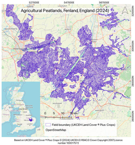
Figure 1.
Study area map showing the location of agricultural peatlands in the East Anglian region of England and the field boundaries demarcating individual fields. The extent of the agricultural peatlands was based on the Peaty Soils Location map of England by BGS and NSRI.
As a result, the UK’s net-zero pathways include restoring 25% of lowland peat, sustainably managing 75% of croplands, and rewetting 50% of grasslands by 2050 [46,47]. At the national level, policymakers have introduced a range of interventions to support the sustainable management of lowland peatlands, including a focus on proper inventory (extent and mapping), formation of the Lowland Agricultural Peat Task Force, and agri-environment schemes (including paludiculture grants) to encourage water table management and restoration efforts in the Fens [26,48]. On the ground, farmers are responsible for managing local drainage systems (e.g., subsurface drainage tiles and field ditches) to maintain optimal conditions for crop growth and implement soil conservation practices based on soil health (e.g., cover cropping, hedgerow establishment, and crop rotation, etc.) to mitigate soil erosion and sustain productivity [49]. Thus, an effective monitoring system within this area would need to operate at a field scale, provide long-term monitoring capability, and provide full coverage of the area, which includes both croplands and grasslands on lowland peatlands.
2.2. Framework Development
This section outlines the development of the framework used in this study, which consists of three key elements (shown in Figure 2 below):
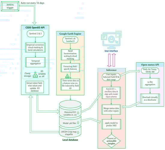
Figure 2.
Overview of the operational CO2 flux monitoring framework. The system integrates EO, meteorological, and ancillary data through automated workflows, enabling user-driven inference of Net Ecosystem Exchange (NEE) at the field scale via a web-based interface.
- Auto-updating EO database: A database of EO variables and ancillary data, periodically updated with recent observations, enabling both historical and near-real-time monitoring through automated workflows triggered at predefined intervals.
- User-driven data integration and inferencing: Based on user-defined inputs (e.g., location, time), the system fetches relevant EO, ancillary, and meteorological data and integrates them into the model pipeline. The pre-trained model processes the input data to produce the Net Ecosystem Exchange of CO2 output.
- User interface: A web-based interactive Graphical User Interface (GUI) that allows users to select a field and a temporal window. It visualizes the model output as actionable insights.
2.3. Pre-Trained Model and Expected Inputs
We used a pre-trained EO-based ML model for predicting CO2 fluxes (Gross Ecosystem Productivity (GEP), Total Ecosystem Respiration (TER), and Net Ecosystem Exchange of CO2 (NEE)) in drained peatlands of East Anglia developed by Khan et al. (2025) [31]. The Random Forest Regressor model was trained on Eddy Covariance flux tower data (available from The UK Centre for Ecology & Hydrology (UKCEH) Environmental Information Data Centre (EIDC)) from six agricultural and grasslands fields of drained lowland peatlands in East Anglia (see Figure S1 in Supplementary Materials). The model used a combination of input variables from different sources and of different categories: vegetation and moisture indices, biometeorological variables, soil organic carbon content, and land use categories. A detailed list of input variables used in the original model is provided in Table 1 (below). The model supports biweekly prediction of GEP, TER, and NEE (= TER-GEP) in gC/m2/day. The predictive uncertainty in NEE outputs was quantified by propagating the uncertainty of component fluxes (GEP and TER) using the Monte Carlo propagation of error. The uncertainty of GEP and TER was based on quantiles (5th and 95th) of prediction distribution from the RF model. More details on model training and uncertainty quantification are given in the Supplementary Materials (Sections S1 and S2).

Table 1.
Categorical list of input variables required by the pre-trained RFR model for NEE inference, including the expected ranges and data source used during the training.
The model achieved an average predictive accuracy of 77%, with an R2 value of 0.79 and a root mean square error (RMSE) of 1.51 gC/m2/day (normalized RMSE by range of observed flux values = 8.67%). The predictive uncertainty of the model across the East Anglian Fens ranged from ±0.29 to ±1.28 kgC/m2 in 2023. The trained model, saved as a .pkl file, was integrated directly into the operational framework for inferencing.
2.4. Earth Observation Database
To enable real-time inference in response to user queries, it is essential that model input data be readily accessible within a minimal latency window. Although on-the-fly generation of inputs (e.g., filtering, feature extraction, and formatting of EO data) is feasible, without paid tools or infrastructure, such operations can introduce significant delays (e.g., often exceeding 10 min per query using CDSE catalogue APIs) and put limitations on user requests [17]. To mitigate this, we implement a hybrid approach which includes precomputing and storing field-wise model inputs from historical EOs and an automated processing chain to periodically update this dataset with the latest available EO data. As a result, model inference only requires input retrieval rather than full download and preprocessing at the time of user request, substantially reducing computation time and improving system response time.
2.4.1. Historical EO Data
We used Google Earth Engine (GEE) to acquire and process historical satellite data going back to 2017, a time period selected to align with the availability of both Sentinel-2 and Landsat 8 data on the cloud-based platform. GEE provides access to a vast archive of analysis-ready satellite data and allows users to perform complex computations without the need for extensive local processing power [54]. This significantly reduces both the time and technical effort required to generate historical time series over large areas, which remains a popular use of the platform [55]. In our case, generating field-wise time series with a defined temporal aggregation period was completed efficiently using GEE’s native spatiotemporal (reducer) functions and batch processing. Additionally, it provided flexible export functionalities that allow users to define the structure and tailored formatting (e.g., field-wise CSVs, time-averaged summaries, etc.) suitable for downstream analytical workflows.
The date range 2017–2025 was selected based on the availability of data from both sensors on the platform. The bands were harmonized using Empirical Linear Correction to match Sentinel 2 SR to that of Landsat 8 (e.g., RedL8 = a⋅RedSen2A + b) (additional details in Section S3, Table S1, Supplementary Materials). Harmonized surface reflectance bands were then used to calculate key vegetation indices (NDVI, EVI, and NDMI). Land Surface Temperature (LST) was estimated using a publicly available GEE-based implementation of the Statistical Mono-Window (SMW) algorithm developed by [50], which calculates LST from Landsat thermal data via a linear regression with Top Of Atmosphere brightness temperatures in a single Thermal Infrared channel [56,57]. Using the UKCEH Land Cover ® Plus: Crops map, field-wise (polygon-based) zonal statistics were performed to extract average values for each variable at 14-day intervals. These were exported as structured Comma-Separated Value (CSV) files indexed by a unique field ID for each field. These field IDs are used as a constant identifier (fieldID) throughout this workflow to identify individual fields.
2.4.2. Recent EO Data
- (i)
- Data download using CDSE OpenEO API
OpenEO is an open source interface that standardizes access to EO data and processing services across multiple platforms [58,59], making it particularly useful for remote sensing-based operational frameworks. When combined with the Copernicus Data Space Ecosystem (CDSE) archive, the openEO API offers the flexibility and tools needed to develop tailored processing chains and their integration with custom workflows [60]. While the Google Earth Engine (GEE) API can also be used for automated, periodic data download and processing, it often requires additional steps, such as manual export configurations or complex workarounds involving Google Drive or Cloud Storage [17]. It also provides limited transparency around computational usage and quota limits. In contrast, OpenEO offers a greater backend flexibility, larger download bandwidth, and easy integration into automated pipelines, making it better suited for integration into monitoring systems. For our purpose, using OpenEO API for building an operational system can reduce development time, enhance reproducibility, and future-proof workflows against backend changes [59]. The free tier of OpenEO API offers 10,000 credits each month, which are generally enough for basic data downloading and processing twice a month for a regional-scale operation.
For EO-based inputs used in the original model, vegetation indices and LST, we used Sentinel-2 Level-2A and Sentinel-3 SLSTR Level-2 Land Surface Temperature (LST) data from the Copernicus Dataspace via the OpenEO Python client (0.37.0), respectively. This reduced the processing time required for modelling LST separately. The initial processing steps were similar to those used for processing historical EO data from GEE: filtering data through datacubes, band harmonization, applying scaling factors, unit conversion (LST from K to °C), and temporal aggregation. However, instead of exporting field-wise values for each feature, which can take a substantial amount of time and credits on OpenEO, we download 14-day composites as tiff files and extracted field-wise features, which were merged with existing tabular datasets containing prior observations (as demonstrated in Figure 3).
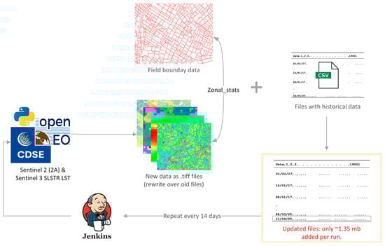
Figure 3.
Shows the automated workflow using Jenkins for biweekly update of EO data within the framework.
- (ii)
- CI/CD using Jenkins
To ensure the system remains up to date with new data without the need for human intervention, the OpenEO API processing chain was fully automated using Continuous Integration/Deployment (CI/CD) [61] in Jenkins [61,62], an off-the-shelf, open source continuous integration (CI) system that supports extensible pipelines and plugins, making it well-suited for scientific data tasks [62]. In our setup, the primary automation pipeline is triggered biweekly via a cron schedule to perform a sparse checkout of the required directories from GitLab, which is the version control system used. It creates a Python virtual environment (or activates if already present), runs the OpenEO-based data download and processing script (described in Section 2.4.2 (i)), and updates the local database. Temporary .tiff files are overwritten each cycle to minimize storage use, and only the extracted information is stored permanently. The secondary pipeline is triggered automatically upon completion of the first; this stage synchronizes data folders, commits updated files to GitLab, and pushes them to the main branch.
2.5. Additional Model Inputs: Meteorological, Soil, and Land Use Data
In addition to Earth Observation (EO) variables, the model requires two other categories of input: (a) meteorological data and (b) soil and land use information. Meteorological data is retrieved dynamically at inference time using the Open-Meteo API [63], a free and open source weather data service designed for non-commercial use. Due to the API’s fast response time, this data is not pre-stored but is instead fetched in real-time based on the user’s query parameters (e.g., location and date window). The Historical Weather API provided by Open-Meteo is based on reanalysis datasets powered by the ECMWF Integrated Forecasting System (IFS), using 0z and 12z simulation runs at ~9 km spatial resolution. Section S4 (Supplementary Materials) shows the comparison between the meteorological input from Open-Meteo and the inputs used in the original model training (Table 1).
Field-level soil and land use information is sourced from the same datasets used during model training (Table 1) and stored locally in a structured .csv files.
2.6. Front-End
For the front-end GUI development, we used Python-based NiceGUI to establish a backend server and Leaflet JavaScript library to create an interactive map of field boundaries. Vanilla JS was used to handle all user interactions and logic without the need for large frameworks. Options were provided for the users to select fields and date ranges to run an analysis. Charts.js. was used to create colour-coded, interactive time series plots of the predicted NEE. The front-end was connected to the backend using a FastAPI web framework. It provides the REST services that allows the system functionality to be accessible from a public domain. Figure 4 (below) highlights all key components of the front-end.
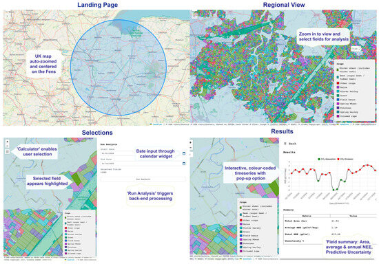
Figure 4.
The web-based front-end for field-scale analysis. It allows users to zoom into the Fens, England, explore and select fields of interest (Regional View), configure inputs and run analysis (Selections), and view NEE outputs presented as actionable insights through colour-coded, interactive plots and a field summary table (Results).
3. Operational Workflow and User Interaction
This section describes how the different elements of the framework described previously come together for real-time execution initiated by user inputs. The pipeline is initiated when the user clicks the “Run Analysis” button on the front-end, which becomes active after both a field and a date range are selected. This triggers the first step of the processing chain (shown in Figure 5).
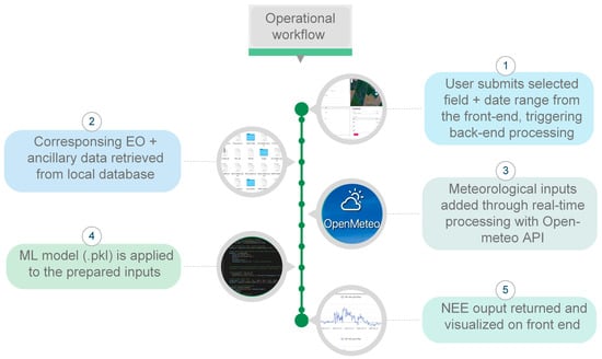
Figure 5.
Shows the operational workflow triggered when a field and date range is submitted by the user on the front-end.
- (i)
- EO, land use, and soil parametersThe workflow begins by accessing the local database to fetch pre-prepared EO, soil, and land use variables. For a user-specified field identifier (fieldID) and date range (start and end dd/mm/yyyy), the relevant variables are extracted from the database (variable set 1, 3, and 4 in Table 1). Each of these inputs is read from locally stored CSV files indexed by fieldID. The corresponding time series are filtered to match the user-specified temporal range and are compiled into an integrated dataset.
- (ii)
- Meteorological parametersThe next step includes the retrieval and integration of the weather data from the Open-Meteo API. The field centroids extracted based on the field identifier selected by the user (fieldID) are used to query the API along with the date range selected (using a freely available script from Open-Meteo website). Hourly data for required variables (Table 1, set 2) are aggregated to 14-day means to align with the EO data and merged into a unified dataset for inference.
- (iii)
- Model inference and output visualization
Once the EO-derived and meteorological inputs are assembled, they are passed to a pre-trained model, stored as serialized pickle (.pkl) files. These represent the GEP and TER components of the ecosystem carbon flux and are used to compute NEE (= TER−GEP). Uncertainty is dynamically estimated following the original model’s Monte Carlo approach (Section 2.3). Predictions and uncertainty values are returned via an API as JSON objects, then visualized in the front-end as biweekly time series along with summary statistics.
4. Use Cases
To demonstrate the utility of our operationalized framework for CO2 flux monitoring in support of field-level management decisions, we first implement a series of use-case scenarios centred on Rosedene Farm (52.52°N, 0.49°E), an intensively managed cropland located in the East Anglian Fens. This site was selected based on the availability of flux tower observations [64] and land management information [65], which allow us to simulate how land managers might interact with the system in real-world decision-making scenarios and validate the outputs. The table below (Table 2.) shows the cropping history of the field between 2017 and 2019, taken from [65].
Table 2.
Cropping history at Rosedene Farm (taken from [65]).
4.1. Scenario 1: Monitoring Crop-Specific CO2 Flux Patterns
(a) Using the web-based front-end, we select Rosedene Farm (field #11367) and specify a date range corresponding to a known cropping season (e.g., 8 April 2017–5 February 2018, the period during which sugar beet was cultivated). Upon submission, the system retrieves and processes the relevant EO and meteorological data, returning a biweekly NEE time series and summary statistics with a response time of 6.06 s. We obtain an average NEE of 1.18 gC/m2/day and a cumulative NEE: 363.94 gC/m2 in the summary section (Figure 6).
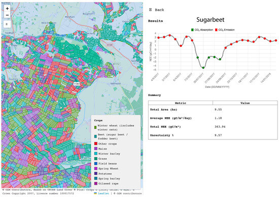
Figure 6.
Screenshot of use-case scenario 1 from the front-end. Top-left section highlights the selected field (Rosedene Farm) on the map of East Anglian agricultural peatlands. The time series plot shows the NEE dynamics from the field during sugar beet cropping season. A clear seasonal trend in NEE can be observed, with the field acting as a CO2 sink (green dots) during the peak growing season (July–September) and remaining a CO2 source (red dots) during the rest of the cropping season.
(b) Repeating the same steps for the potato cropping period (17 May 2019–31 October 2019), the analysis yields an average NEE of 2.94 gC/m2/day and cumulative NEE of 534.62 gC/m2. The user can then compare the differences in seasonal CO2 flux dynamics linked to crop type and phenology (e.g., higher NEE values of potato). Such comparisons could be extended to evaluate the potential benefits of switching to alternative practices such as paludiculture, where carbon emissions are minimized by maintaining a higher soil moisture. This approach has been promoted in the Fens through dedicated policies and grants [66].
4.2. Scenario 2: Comparing Active and Fallow Periods
To examine the impact of bare or fallow periods, the system is queried for a timeframe with no active crop cover (21 June 2018–17 May 2019). Here, the results showed a much higher rate of NEE (3.24 gC/m2/day), with a total of 1.13 kgC released per m2 during this period. This reflects a substantially higher release of CO2 to the atmosphere, underlining the importance of practices such as cover cropping or residue management to minimize off-season emissions. This comparison can enable the practical evaluation of mitigation practices undertaken during the fallow period (e.g., cover cropping, residue management) and can guide farmers in making informed decisions. A figure showing a comparison of outputs from use cases 1 (a and b) and 2, as seen on the front-end, is provided in the Supplementary Materials (Figure S3).
4.3. Scenario 3: Comparing the Effects of Different Land Uses
To demonstrate the spatially scalable application of the tool, a user may query fields from different parts of the Fenland, and of different land use type. We run analyses in the same year (2022) for a cropland site (Redmere Farm; 52.443°N, 0.4195°E; Field ID #8032) and a managed grassland site (Woodwalton Fen (52.46°N, −0.1851°W; Field ID: #8157), both of which have been monitored by flux towers in 2022 [67]. Both sites lie in different parts of the Fenland and are separated by a substantial distance (Figure 7 and Figure S1). Outputs took an average of 6.15 s to generate and clearly differentiate the CO2 flux signatures between cropland and grassland systems, revealing a greater NEE amplitude but lower net emissions in the grassland site compared to the higher temporal variability and net emissions from the cropland site. The colour-coded time series also highlights periods of CO2 absorption (in green), which were substantially longer in the grassland site (Figure 7, (top)). Similar comparisons can help assess the effectiveness of land use change (e.g., cropland-to-grassland conversion), and comparisons between grasslands can help in measuring the impact of rewetting measures proposed for grasslands in the area [46,47], as well as the impact of other agri-environment interventions.
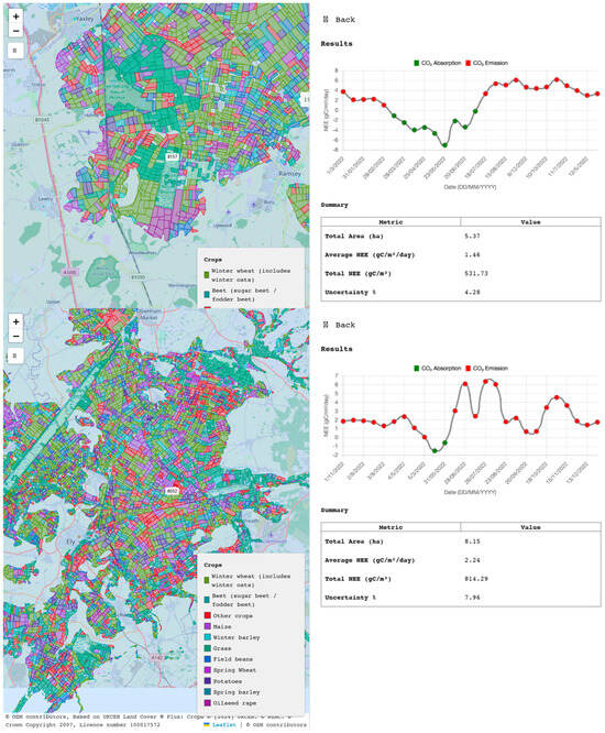
Figure 7.
Screenshots of use-case scenario 3 from the front-end comparing annual NEE dynamics from a grassland (top) and cropland (bottom) site located in different parts of the Fenland. The colour-coded time series provides easy interpretation of CO2 flux dynamics in the fields, including periods of net absorption (green) and emissions (red).
5. Validation
The system’s output was validated against Eddy Covariance (EC) flux tower data from the East Anglian Fens (2017–2023), obtained from the UK Centre for Ecology & Hydrology (UKCEH). The locations of the flux towers and references to the corresponding datasets are provided in the Supplementary Materials (Table S1, Figure S1).
Overall, the system achieved an R2 of 0.76 and a normalized root mean square error (NRMSE) of 8% (RMSE = 1.53 gC/m2/d, normalized by flux ranges), which is comparable to the accuracy of the pre-trained model used (R2 = 0.79, RMSE = 1.51 gC/m2/d, NRMSE = 9%). Figure 8a also illustrates the system’s performance against the observed EC flux data under different use-case scenarios presented in Section 4. Across these scenarios, the system achieved an average R2 of 0.73 and RMSE of 1.44 gC/m2/d (NRMSE = 11%). The system effectively reproduced key temporal trends, including decreases in the Net Ecosystem Exchange (NEE) as plant biomass increases during growing seasons, post-harvest increases in the NEE during fallow periods, and differences in the flux variability and range between grassland and cropland sites (Figure 8a). However, the system struggled to predict the full NEE magnitude during seasonal extremes.
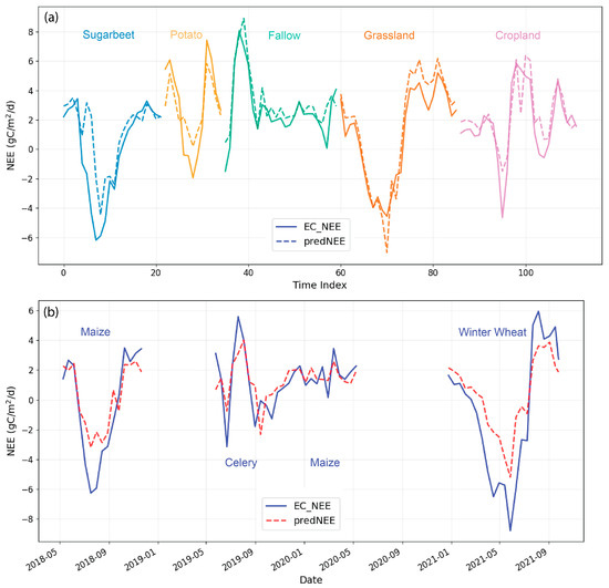
Figure 8.
Time series plots comparing predicted NEE (dashed line) to the observed data from Eddy Covariance flux towers (solid line) for (a) use-case scenarios described in Section 4 and (b) an independent flux tower site (unseen by the model) from East Anglian Fens (Engine Farm; 52.423°N, 0.386°E). Figure highlights the performance of the monitoring system across different sites, land use categories, and management types. Accompanying scatter plot is provided in the Supplementary Materials (Figure S4).
For an independent cropland site not included in model training, the system achieved an R2 of 0.71 and NRMSE of 12% (RMSE = 1.69 gC/m2/d; Figure 8b), consistent with the spatial cross-validation performance of the underlying geoML model (R2 of 0.7, NRMSE = 13%). The predictions captured overall seasonal dynamics across three cropping seasons but showed deviations in peak flux magnitudes and during periods of high fluctuations (e.g., transition period between celery and maize cropping). Based on the above performance metrics, the system retained approximately 98% of the accuracy of the pre-trained model that it operationalized.
6. Discussion
This study demonstrated an adaptable framework for operationalizing and scaling GeoML analytics within Digital Twin infrastructures, thereby enhancing their applicability for decision- and policymaking support. Using the case study of an Earth Observation (EO)-based Machine Learning (ML) model for predicting the Net Ecosystem Exchange (NEE) of CO2 in drained peatlands of England, we deployed the presented framework into a CO2 flux monitoring system and demonstrated how different stakeholders (farmers and policymakers) can use it in various scenarios for field-level land management and monitoring. The CO2 monitoring system, designed to respond to user selections, had a response time of 5.80–6.50 s, an interactive interface, and immediate visual feedback through interpretable plots that distinguish between the emissions and absorption of CO2. These outputs are further contextualized with statistical summaries, facilitating the transformation of raw model outputs into actionable insights. Despite its functionality, the framework remains lightweight, requiring approximately one gigabyte of storage and being readily deployable on local servers. The operational system retained the 98% accuracy (R2 = 0.76; NRMSE = 8%) of the underlying model. The validation and spatial cross-validation against the observed data showed that the system predicts general trends and directions of NEE consistently across varying land use and management types.
The framework’s design prioritizes computational efficiency and flexibility, making it suitable for adaptation across different modelling applications. The input data architecture is hybrid, comprising both archival (non-time-sensitive) and real-time components. This design allows for faster data retrieval and minimizes redundant computation. To optimize data access and storage, the system avoids computationally heavy data formats (such as NetCDF or geoTIFFs) wherever possible. Instead, pre-processed variables are stored as structured CSV files indexed by field ID, and can be easily updated, even by non-experts. The framework leverages freely available libraries and tools for data download, automation, processing, and visualization, ensuring accessibility and reproducibility. Finally, the modular architecture allows for easy reconfiguration of the number, type, and source of the model or its inputs. This makes the framework adaptable to models with different spatial/temporal resolutions, variable needs, and outputs, and reproducible for EO and meteorological data-enabled models for regional and local applications.
The framework can be used to integrate geoML capabilities into larger digital infrastructures, including Digital Twin (DT) systems. In DT systems where multiple models are used to produce distinct outputs, individual workflows can be invoked on demand via front-end queries using containerization [68]. For DT systems that rely on a fusion of modelling approaches to represent a physical system, for example, ML for historical output and simulation models for scenario predictions [69], the framework can operate internally or be embedded within other components without requiring a significant alteration to its data handling or execution logic. Alternatively, these methods can be used together, for example, in the DT system (“Self-Learning Digital Twin for Sustainable Land Management”), where this framework is being used to provide NEE predictions based on observed (historical and near-real-time) EO and meteorological data. The framework is containerized using Docker [70] and integrated within the Digital Twin (DT) environment. User requests, which include climate scenarios, are first filtered to determine the processing path. If the request requires observed-data-based outputs, the framework operates as usual, returning NEE outputs for corresponding dates and field IDs. For requests involving alternative climate scenarios, the framework operates within other (simulation) models and provides bias correction based on observed values. Apart from being connected to a different front-end, the framework operates within the DT without any changes to the processing chains.
Limitations, Practical Considerations, and Future Directions
While the framework demonstrates a strong operational potential, some limitations remain. Firstly, the current framework does not incorporate an automated feedback loop for model retraining or validation. Any model updates require manual intervention by the model developers. This is also required for some of the static datasets used, for example, the land use categories; if classification were to change, they would have to be updated manually, or an additional workflow will need to be implemented for land use classification before the NEE model is applied. This can be based on existing data streams [71] or by adding more satellite data [72]. This also applied to other projects wanting to operate at a field scale but not having access to field boundary information; delineation algorithms for boundary classification [73] can be incorporated into the framework to generate this information autonomously.
Secondly, while .csv files offer simplicity, readability, and ease of integration with metadata (e.g., crop type, field ID, management history) and are a good choice for the scale of application demonstrated in this study, they are less efficient for very large spatial or temporal datasets. For broader-scale deployments, formats like GeoParquet or NetCDF may offer a better performance in terms of efficiency and compression. Thirdly, our framework uses a model exported in pickle (.pkl) file format using joblib, which can have several integration issues and often lacks cross-version compatibility; the use of standardized, platform-independent formats (such as ONNX) for model export may help mitigate these issues in future iterations [74].
Additional considerations relate to the operational scale and frequency of updates in operational geoML. Models requiring more frequent data updates (e.g., weekly) or a wider spatial coverage may exhaust free credits on platforms such as OpenEO before the update workflow is completed. In such cases, a more computationally heavy pipeline might need to be established using catalogue APIs and HTTP GET requests to download data [75] and Python-based processing in the absence of native processing options available with OpenEO. Alternatively, the Google Earth Engine API can be used for downloading field-wise pre-processed data by adding another automating pipeline to download data from Google Drive to the chosen directory and to perform spatial task segmentation to comply with platform processing limits. If the budget allows, paid API services can be considered for extending the allowance within CDSE OpenEO or using Sentinel Hub for more efficient data retrieval and processing.
The accuracy of the predicted fluxes depended strongly on the performance of the underlying model, as expected. Therefore, users should consider the model’s inherent limitations when interpreting system outputs. Firstly, the 14-day temporal aggregation limits the detection of event-driven flux dynamics, as short-lived fluctuations (such as those caused immediately after tillage, fertilizer application, or extreme weather events) are averaged out. Secondly, an insufficient representation of seasonal extremes or specific crop types in the training data may lead to a misclassification of sink/source periods or misestimation of fluxes during peak seasons or for certain crops (e.g., sugar beet, leek [31]). Finally, the uncertainty quantification method (which the system emulates) does not account for uncertainties arising from input data, such as resolution mismatches among datasets or uncertainty due to flux data processing (e.g., gap-filling and flux partitioning). Since the system employs similar input data to the base model, it retains a comparable accuracy overall, but the slight deviations observed likely reflect discrepancies among input meteorological datasets. Although the data from the Open-Meteo API shows a good alignment with the CHESS-met data used at the training time, (see Supplementary Materials, Section S4), the coarser spatial resolution can affect the accuracy of fluxes in heterogenous landscapes [76].
Considering the validation results and model limitations, the system is best suited for monitoring long-term trends in cumulative NEE, reflecting whether a site acts as a net carbon source or sink, evaluating management-induced changes that persist beyond short-term fluctuations, and comparing seasonal flux cycles across different land use scenarios, rather than for estimating short-term, absolute flux magnitudes. Consequently, more comprehensive uncertainty quantification and sensitivity analysis of meteorological parameters would be necessary before the flux magnitudes could be used for reporting purposes. Future improvements could be achieved by retraining the underlying model with additional flux tower data encompassing a wider range of management practices, which would enhance both accuracy and generalizability.
A promising avenue for future development also lies in the integration of explainable artificial intelligence (XAI) methods [77] with operational geoML to enhance the transparency and interpretability of model outputs related to CO2 fluxes. For instance, in scenario 1 of the presented use case, being able to decipher if the differences in the NEE of sugar beet and potatoes are solely driven by phenology and productivity variables or are a result of varying meteorological conditions would enable more accurate and informed interventions. The front-end interface can also be expanded to deliver more contextual information to users, such as maps highlighting areas of concern (e.g., [78]), or to recommend interventions based on the known cropping history, soil information, and historical flux dynamics of a certain field.
7. Conclusions
The operationalizing framework and its real-world applicability demonstrated in this study offer a flexible and efficient approach for implementing geoML in Digital Twin systems for CO2 monitoring and related policymaking efforts. Designed for a seamless integration into Digital Twin systems, its lightweight structure, open source implementation, and modular design make it a scalable and accessible solution for environmental monitoring and decision support, particularly for regional and local applications. For studies operating on significantly larger spatial or temporal scales than the one presented here, we discussed how additional infrastructure or emerging tools and services can be used to address any limitations related to automation, data format scalability, and API constraints. Overall, the framework’s architecture and design choices lay a strong foundation for bridging the gap between research and practice by advancing the operational deployment of geoML models for CO2 flux monitoring and serve as an adaptable template for use in future environmental Digital Twin systems aimed at supporting sustainable land management, carbon monitoring, and broader climate resilience efforts.
Supplementary Materials
The following supporting information can be downloaded at https://www.mdpi.com/article/10.3390/rs17213615/s1. Figure S1: Location of training and validation sites used for the underlying model; Table S1: Empirical calibration equations for harmonizing Landsat and Sentinel data; Figure S2: Comparison of meteorological variables derived from Open-Meteo API to those derived from CHESS-met dataset; Table S2: Description of Eddy Covariance Flux Tower data used for system validation; Figure S3: Comparison of use-case scenarios presented in Section 4 of the study; Figure S4: Scatter plot complementary to time-series plot (Figure 8a) in the study.
Author Contributions
Conceptualization, A.K.; methodology, A.K., M.A. and A.M.; software, A.K., M.A. and A.M.; validation, A.K.; formal analysis, A.K.; data curation, A.K.; writing—original draft preparation, A.K.; writing—review and editing, A.M., A.A. and H.B.; visualization, A.K., M.A. and A.M.; supervision, H.B. and A.A.; project administration, H.B.; funding acquisition, H.B. and A.A. All authors have read and agreed to the published version of the manuscript.
Funding
This research was funded by the Engineering and Physical Sciences Research Council (EPSRC) and UK Research and Innovation (UKRI), grant number EP/Y00597X/1.
Data Availability Statement
Code is available at https://gitlab.com/twinlandai/twinland_eo.git (last accessed 23 October 2025).
Acknowledgments
H.B. was supported by the Natural Environment Research Council (NERC) under the National Centre for Earth Observation (NCEO)’s Long-Term Strategic Science funding stream. We gratefully acknowledge the Eddy Covariance (EC) CO2 flux datasets compiled by Cooper et al. (2024) [67], Cumming et al. (2020) [64], Kelvin et al. (2021) [79], Morrison et al. (2020) [80], and Morrison et al. (2021) [81] containing data supplied by UK Centre for Ecology & Hydrology (available under the Open Government Licence v3 (OGL)), which are also based on the work of Cumming (2018) [82], Evans et al. (2016) [83], Morrison (2013) [84], Morrison et al. (2013) [85], and Newman (2022) [65], and datasets compiled by Maria B. Mills and Arina Machine. We thank Jorg Kaduk, Ivan Reading, Hibist Kassa, Fang Chen, Noel Clancy, Gavers Oppong, Ursula Davis, Stephen Wright, John Maltby, Maria Touri, Huiyu Zhou, Corentin Houpert, Craig Bower, Kevin Tansey, Rob Parker, Harjinder Sembhi, Neil Humpage, Pat Heslop-Harrison, Hess Ekkeh, and Susan E. Page for their valuable discussions and insights throughout this project.
Conflicts of Interest
The authors declare no conflicts of interest.
References
- Alotaibi, E.; Nassif, N. Artificial intelligence in environmental monitoring: In-depth analysis. Discov. Artif. Intell. 2024, 4, 84. [Google Scholar] [CrossRef]
- Gao, S. Geospatial Artificial Intelligence (GeoAI); Oxford University Press: New York, NY, USA, 2021. [Google Scholar]
- Yuan, Q.; Shen, H.; Li, T.; Li, Z.; Li, S.; Jiang, Y.; Xu, H.; Tan, W.; Yang, Q.; Wang, J.; et al. Deep learning in environmental remote sensing: Achievements and challenges. Remote Sens Env. 2020, 241, 111716. [Google Scholar] [CrossRef]
- Victor, N.; Maddikunta, P.K.R.; Mary, D.R.K.; Murugan, R.; Chengoden, R.; Gadekallu, T.R.; Rakesh, N.; Zhu, Y.; Paek, J. Remote Sensing for Agriculture in the Era of Industry 5.0—A Survey. IEEE J. Sel. Top. Appl. Earth Obs. Remote Sens. 2024, 17, 5920–5945. [Google Scholar] [CrossRef]
- Wu, B.; Zhang, M.; Zeng, H.; Tian, F.; Potgieter, A.B.; Qin, X.; Yan, N.; Chang, S.; Zhao, Y.; Dong, Q.; et al. Challenges and opportunities in remote sensing-based crop monitoring: A review. Natl. Sci. Rev. 2022, 10, nwac290. [Google Scholar] [CrossRef]
- Fassnacht, F.E.; White, J.C.; Wulder, M.A.; Næsset, E. Remote sensing in forestry: Current challenges, considerations and directions. Forestry 2023, 97, 11–37. [Google Scholar] [CrossRef]
- Olawade, D.B.; Wada, O.Z.; Ige, A.O.; Egbewole, B.I.; Olojo, A.; Oladapo, B.I. Artificial intelligence in environmental monitoring: Advancements, challenges, and future directions. Hyg. Environ. Health Adv. 2024, 12, 100114. [Google Scholar] [CrossRef]
- Porcar-Castell, A.; Mac Arthur, A.; Rossini, M.; Eklundh, L.; Pacheco-Labrador, J.; Anderson, K.; Balzarolo, M.; Martín, M.; Jin, H.; Tomelleri, E.; et al. EUROSPEC: At the interface between remote-sensing and ecosystem CO2 flux measurements in Europe. Biogeosciences 2015, 12, 6103–6124. [Google Scholar] [CrossRef]
- Wang, T.; Zhang, Y.; Yue, C.; Wang, Y.; Wang, X.; Lyu, G.; Wei, J.; Yang, H.; Piao, S. Progress and challenges in remotely sensed terrestrial carbon fluxes. Geo Spat. Inf. Sci. 2025, 28, 1–21. [Google Scholar] [CrossRef]
- Jung, M.; Schwalm, C.; Migliavacca, M.; Walther, S.; Camps-Valls, G.; Koirala, S.; Anthoni, P.; Besnard, S.; Bodesheim, P.; Carvalhais, N. Scaling carbon fluxes from eddy covariance sites to globe: Synthesis and evaluation of the FLUXCOM approach. Biogeosciences 2020, 17, 1343–1365. [Google Scholar] [CrossRef]
- Peters, W.; Jacobson, A.R.; Sweeney, C.; Andrews, A.E.; Conway, T.J.; Masarie, K.; Miller, J.B.; Bruhwiler, L.M.; Pétron, G.; Hirsch, A.I. An atmospheric perspective on North American carbon dioxide exchange: CarbonTracker. Proc. Natl. Acad. Sci. USA 2007, 104, 18925–18930. [Google Scholar] [CrossRef] [PubMed]
- Gottschalk, P.; Kalhori, A.; Li, Z.; Wille, C.; Sachs, T. Monitoring cropland daily carbon dioxide exchange at field scales with Sentinel-2 satellite imagery. Biogeosciences 2024, 21, 3593–3616. [Google Scholar] [CrossRef]
- Zhuravlev, R.; Dara, A.; Santos, A.L.D.d.; Demidov, O.; Burba, G. Globally scalable approach to estimate net ecosystem exchange based on remote sensing, meteorological data, and direct measurements of eddy covariance sites. Remote Sens. 2022, 14, 5529. [Google Scholar] [CrossRef]
- Tramontana, G.; Jung, M.; Schwalm, C.R.; Ichii, K.; Camps-Valls, G.; Ráduly, B.; Reichstein, M.; Arain, M.A.; Cescatti, A.; Kiely, G. Predicting carbon dioxide and energy fluxes across global FLUXNET sites with regression algorithms. Biogeosciences 2016, 13, 4291–4313. [Google Scholar] [CrossRef]
- Kolltveit, A.B.; Li, J. Operationalizing machine learning models: A systematic literature review. In Proceedings of the 1st Workshop on Software Engineering for Responsible AI, Pittsburgh, PA, USA, 17 May 2022; pp. 1–8. [Google Scholar]
- Shi, H.; Luo, G.; Hellwich, O.; Xie, M.; Zhang, C.; Zhang, Y.; Wang, Y.; Yuan, X.; Ma, X.; Zhang, W. Variability and uncertainty in flux-site scale net ecosystem exchange simulations based on machine learning and remote sensing: A systematic evaluation. Biogeosci. Discuss. 2022, 19, 3739–3756. [Google Scholar] [CrossRef]
- Gomes, V.C.; Queiroz, G.R.; Ferreira, K.R. An overview of platforms for big earth observation data management and analysis. Remote Sens. 2020, 12, 1253. [Google Scholar] [CrossRef]
- Liang, X.; Yu, S.; Meng, B.; Wang, X.; Yang, C.; Shi, C.; Ding, J. Multi-Source Remote Sensing and GIS-Driven Forest Carbon Monitoring for Carbon Neutrality: Integrating Data, Modeling, and Policy Applications. Forests 2025, 16, 971. [Google Scholar] [CrossRef]
- Oleszczuk, R.; Regina, K.; Szajdak, L.; Höper, H.; Maryganova, V. Impacts of agricultural utilization of peat soils on the greenhouse gas balance. In Peatlands and Climate Change; International Peat Society: Jyväskylä, Finland, 2008; pp. 70–97. [Google Scholar]
- Hooijer, A.; Page, S.; Jauhiainen, J.; Lee, W.A.; Lu, X.X.; Idris, A.; Anshari, G. Subsidence and carbon loss in drained tropical peatlands. Biogeosciences 2012, 9, 1053–1071. [Google Scholar] [CrossRef]
- Conchedda, G.; Tubiello, F.N. Drainage of organic soils and GHG emissions: Validation with country data. Earth Syst. Sci. Data Discuss. 2020, 12, 3113–3137. [Google Scholar] [CrossRef]
- Hooijer, A.; Page, S.; Canadell, J.G.; Silvius, M.; Kwadijk, J.; Wösten, H.; Jauhiainen, J. Current and future CO 2 emissions from drained peatlands in Southeast Asia. Biogeosciences 2010, 7, 1505–1514. [Google Scholar] [CrossRef]
- Miettinen, J.; Shi, C.; Liew, S.C. Two decades of destruction in Southeast Asia’s peat swamp forests. Front. Ecol. Environ. 2012, 10, 124–128. [Google Scholar] [CrossRef]
- Evans, C.; Artz, R.; Moxley, J.; Smyth, M.A.; Taylor, E.; Archer, E.; Burden, A.; Williamson, J.; Donnelly, D.; Thomson, A.; et al. Implementation of an Emissions Inventory for UK Peatlands; Centre for Ecology and Hydrology: Wallingford, UK, 2017. [Google Scholar]
- Reed, M.; Buckmaster, S.; Moxey, A.; Keenleyside, C.; Robinson, G.; Slee, B. Policy Options for Sustainable Management of UK Peatlands; IUCN: Gland, Switzerland, 2010. [Google Scholar]
- Lloyd, I.L.; Thomas, V.; Ofoegbu, C.; Bradley, A.V.; Bullard, P.; D’Acunha, B.; Delaney, B.; Driver, H.; Evans, C.D.; Faulkner, K.J. State of knowledge on UK agricultural peatlands for food production and the net zero transition. Sustainability 2023, 15, 16347. [Google Scholar] [CrossRef]
- Evans, C.D.; Peacock, M.; Baird, A.J.; Artz, R.; Burden, A.; Callaghan, N.; Chapman, P.J.; Cooper, H.M.; Coyle, M.; Craig, E. Overriding water table control on managed peatland greenhouse gas emissions. Nature 2021, 593, 548–552. [Google Scholar] [CrossRef] [PubMed]
- Eickenscheidt, T.; Heinichen, J.; Drösler, M. The greenhouse gas balance of a drained fen peatland is mainly controlled by land-use rather than soil organic carbon content. Biogeosciences 2015, 12, 5161–5184. [Google Scholar] [CrossRef]
- Monteverde, S.; Healy, M.G.; O’Leary, D.; Daly, E.; Callery, O. Management and rehabilitation of peatlands: The role of water chemistry, hydrology, policy, and emerging monitoring methods to ensure informed decision making. Ecol. Inform. 2022, 69, 101638. [Google Scholar] [CrossRef]
- Girkin, N.T.; Burgess, P.J.; Cole, L.; Cooper, H.V.; Honorio Coronado, E.; Davidson, S.J.; Hannam, J.; Harris, J.; Holman, I.; McCloskey, C.S. The three-peat challenge: Business as usual, responsible agriculture, and conservation and restoration as management trajectories in global peatlands. Carbon Manag. 2023, 14, 2275578. [Google Scholar] [CrossRef]
- Khan, A.; Ali, M.; Kaduk, J.; Anjum, A.; Balzter, H. Upscaling CO2 fluxes from agricultural drained lowland peatlands in England using remote sensing and machine learning. Remote Sens. Appl. Soc. Environ. 2025, 40, 101728. [Google Scholar] [CrossRef]
- Fu, D.; Chen, B.; Zhang, H.; Wang, J.; Black, T.A.; Amiro, B.D.; Bohrer, G.; Bolstad, P.; Coulter, R.; Rahman, A.F. Estimating landscape net ecosystem exchange at high spatial–temporal resolution based on Landsat data, an improved upscaling model framework, and eddy covariance flux measurements. Remote Sens. Environ. 2014, 141, 90–104. [Google Scholar] [CrossRef]
- Spinosa, A.; Fuentes-Monjaraz, M.A.; El Serafy, G. Assessing the use of Sentinel-2 data for spatio-temporal upscaling of flux tower gross primary productivity measurements. Remote Sens. 2023, 15, 562. [Google Scholar] [CrossRef]
- Junttila, S.; Kelly, J.; Kljun, N.; Aurela, M.; Klemedtsson, L.; Lohila, A.; Nilsson, M.; Rinne, J.; Tuittila, E.S.; Vestin, P. Upscaling Northern Peatland CO2 fluxes using satellite remote sensing data. Remote Sens. 2021, 13, 818. [Google Scholar] [CrossRef]
- Araújo, S.O.; Peres, R.S.; Barata, J.; Lidon, F.; Ramalho, J.C. Characterising the agriculture 4.0 landscape—Emerging trends, challenges and opportunities. Agronomy 2021, 11, 667. [Google Scholar] [CrossRef]
- Lu, B.; Francescutto, L.; Howie, S.; Lin, H.; Wu, Q.; Hedley, N.; Jamali, A.; McDonald, I. Exploring the concept of digital twins of wetlands for supporting ecosystem monitoring and management. Big Earth Data 2025, 1–31. [Google Scholar] [CrossRef]
- Jones, D.; Snider, C.; Nassehi, A.; Yon, J.; Hicks, B. Characterising the Digital Twin: A systematic literature review. CIRP J. Manuf. Sci. Technol. 2020, 29, 36–52. [Google Scholar] [CrossRef]
- Purcell, W.; Neubauer, T. Digital Twins in Agriculture: A State-of-the-art review. Smart Agric. Technol. 2023, 3, 100094. [Google Scholar] [CrossRef]
- Grieves, M. Digital twin: Manufacturing excellence through virtual factory replication. White Pap. 2014, 1, 1–7. [Google Scholar]
- Purcell, W.; Neubauer, T.; Mallinger, K. Digital Twins in agriculture: Challenges and opportunities for environmental sustainability. Curr. Opin. Environ. Sustain. 2023, 61, 101252. [Google Scholar] [CrossRef]
- Chauhan, D.; Bahad, P.; Jain, R. Digital Twins-enabled model for Smart Farming. In Digital Twins for Smart Cities and Villages; Elsevier: New York, NY, USA, 2025; pp. 465–487. [Google Scholar]
- Natural England NE424:NCA Profile: 46. The Fens. 2015. Available online: https://publications.naturalengland.org.uk/publication/6229624 (accessed on 15 June 2025).
- UK Met Office Monthly, Seasonal and Annual Total Precipitation/Temperature Amount for East Anglia. Available online: https://www.metoffice.gov.uk/research/climate/maps-and-data/uk-and-regional-series (accessed on 23 October 2025).
- Morris, J.; Graves, A.; Angus, A.; Hess, T.; Lawson, C.; Camino, M.; Truckell, I.; Holman, I. Restoration of Lowland Peatland in England and Impacts on Food Production and Security; Report to Natural England; Cranfield University: Bedford, UK, 2010. [Google Scholar]
- Rhymes, J.; Stockdale, E.; Napier, B.; Williamson, J.; Morton, D.; Dearlove, E.; Staley, J.; Young, H.; Thomson, A.; Evans, C. The Future of UK Vegetable Production–Technical Report; WWF-UK: Woking, UK, 2023. [Google Scholar]
- CCC (a) The Sixth Carbon Budget: The UK’s Path to Net Zero. 2020. Available online: https://www.theccc.org.uk/publication/sixth-carbon-budget/ (accessed on 7 July 2025).
- CCC (b) Land Use: Policies for a Net Zero UK. 2020. Available online: https://www.theccc.org.uk/publication/land-use-policies-for-a-net-zero-uk/ (accessed on 7 July 2025).
- UK Government England Peat Action Plan. 2021. Available online: https://www.gov.uk/government/publications/england-peat-action-plan (accessed on 15 June 2025).
- Page, S.; Baird, A.; Cumming, A.; High, K.E.; Kaduk, J.; Evans, C. An assessment of the societal impacts of water level management on lowland peatlands in England and Wales: Report to Defra for Project SP1218: Managing agricultural systems on lowland peat for decreased greenhouse gas emissions whilst maintaining agricultural productivity. 2020. Available online: https://lowlandpeat.ceh.ac.uk/sites/default/files/2022-07/Societal-Impacts-Report-March-2020.pdf (accessed on 23 October 2025).
- Ermida, S.L.; Soares, P.; Mantas, V.; Göttsche, F.; Trigo, I.F. Google Earth Engine Open-Source Code for Land Surface Temperature Estimation from the Landsat Series. Remote Sens. 2020, 12, 1471. [Google Scholar] [CrossRef]
- Robinson, E.L.; Blyth, E.M.; Clark, D.B.; Comyn-Platt, E.; Rudd, A.C.; Wiggins, M. Climate Hydrology and Ecology Research Support System Meteorology Dataset for Great Britain (1961–2019) [CHESS-Met]; NERC EDS Environmental Information Data Centre: Edinburgh, UK, 2023. [Google Scholar] [CrossRef]
- Levy, P.E. Daily Soil Moisture Maps for the UK (2016–2023) at 2 km Resolution; NERC EDS Environmental Information Data Centre: Edinburgh, UK, 2024. [Google Scholar] [CrossRef]
- Khamis, D.; Smith, R.; Fry, M.; Evans, J. Modelled Daily Soil Moisture and Soil Temperature at 1km Resolution Across the UK mainland, 1965–2018; NERC EDS Environmental Information Data Centre: Edinburgh, UK, 2024. [Google Scholar] [CrossRef]
- Gorelick, N.; Hancher, M.; Dixon, M.; Ilyushchenko, S.; Thau, D.; Moore, R. Google Earth Engine: Planetary-scale geospatial analysis for everyone. Remote Sens. Environ. 2017, 202, 18–27. [Google Scholar] [CrossRef]
- Tamiminia, H.; Salehi, B.; Mahdianpari, M.; Quackenbush, L.; Adeli, S.; Brisco, B. Google Earth Engine for geo-big data applications: A meta-analysis and systematic review. ISPRS J. Photogramm. Remote Sens. 2020, 164, 152–170. [Google Scholar] [CrossRef]
- Sun, D.; Pinker, R.T.; Basara, J.B. Land surface temperature estimation from the next generation of Geostationary Operational Environmental Satellites: GOES M–Q. J. Appl. Meteorol. 2004, 43, 363–372. [Google Scholar] [CrossRef]
- Duguay-Tetzlaff, A.; Bento, V.A.; Göttsche, F.M.; Stöckli, R.; Martins, J.P.; Trigo, I.; Olesen, F.; Bojanowski, J.S.; Da Camara, C.; Kunz, H. Meteosat land surface temperature climate data record: Achievable accuracy and potential uncertainties. Remote Sens. 2015, 7, 13139–13156. [Google Scholar] [CrossRef]
- Pebesma, E.; Wagner, W.; Schramm, M.; Alexandra, V.B.; Christoph, P.; Neteler, M.; Reiche, J.; Verbesselt, J.; Dries, J.; Goor, E. OpenEO: A Common, Open Source Interface Between Earth Observation Data Infrastructures and Front-End Applications; Zenodo/CERN: Geneva, Switzerland, 2017. [Google Scholar]
- Schramm, M.; Pebesma, E.; Milenković, M.; Foresta, L.; Dries, J.; Jacob, A.; Wagner, W.; Mohr, M.; Neteler, M.; Kadunc, M. The openeo api–harmonising the use of earth observation cloud services using virtual data cube functionalities. Remote Sens. 2021, 13, 1125. [Google Scholar] [CrossRef]
- Milcinski, G.; Bojanowski, J.; Clarijs, D.; de la Mar, J. Copernicus Data Space Ecosystem-Platform That Enables Federated Earth Observation Services and Applications. In Proceedings of the IGARSS 2024-2024 IEEE International Geoscience and Remote Sensing Symposium, Athens, Greece, 7–12 July 2024; pp. 875–877. [Google Scholar]
- Da Gião, H.; Flores, A.; Pereira, R.; Cunha, J. Chronicles of CI/CD: A Deep Dive into its Usage Over Time. arXiv 2024, arXiv:2402.17588. [Google Scholar] [CrossRef]
- Moutsatsos, I.K.; Hossain, I.; Agarinis, C.; Harbinski, F.; Abraham, Y.; Dobler, L.; Zhang, X.; Wilson, C.J.; Jenkins, J.L.; Holway, N. Jenkins-CI, an open-source continuous integration system, as a scientific data and image-processing platform. SLAS Discov. Adv. Life Sci. RD 2017, 22, 238–249. [Google Scholar] [CrossRef]
- Zippenfenig, P. Open-Meteo.com Weather API. 2024. Available online: https://doi.org/10.5281/zenodo.14582479 (accessed on 23 October 2025).
- Cumming, A.M.J.; Newman, T.R.; Benson, S.J.; Balzter, H.; Evans, C.; Jones, D.; Kaduk, J.; Morrison, R.; Page, S. Eddy Covariance Measurements of Carbon Dioxide, Energy and Water Flux at an Intensively Cultivated Lowland Deep Peat Soil, East Anglia, UK, 2012 to 2020. 2020. Available online: https://catalogue.ceh.ac.uk/documents/13896773-01e5-48e6-bfab-c319de46b221 (accessed on 23 October 2025).
- Newman, T.R. Impacts of Long Term Drainage and Agriculture on the Carbon Dynamics of Fen Peatlands in East Anglia, UK; University of Leicester: Leicester, UK, 2022. [Google Scholar]
- Khosravi, F.; Clough, J.A.; Lindsay, R.A. Paludiculture in the UK: A paradigm shift in agricultural practice and farmers’ perceptions. Mires Peat 2025, 32, 22. [Google Scholar]
- Cooper, H.M.; Bodo, A.; Burden, A.; Callaghan, N.; Crabtree, D.E.; Cumming, A.; D’Acunha, B.; Evans, C.; Journeaux, K.; Jovani, J.; et al. Meteorology, Soil Physics, and Eddy Covariance Measurements of Carbon Dioxide, Energy, and Water Exchange from a Distributed Network of Sites Across England and Wales, 2018–2023. 2024. Available online: https://nora.nerc.ac.uk/id/eprint/537424/ (accessed on 23 October 2025).
- Choi, Y.; Roy, B.; Nguyen, J.; Ahmad, R.; Maghami, I.; Nassar, A.; Li, Z.; Castronova, A.M.; Malik, T.; Wang, S.; et al. Comparing containerization-based approaches for reproducible computational modeling of environmental systems. Environ. Model. Softw. 2023, 167, 105760. [Google Scholar] [CrossRef]
- Malakuti, S.; Borrison, R.; Kotriwala, A.; Kloepper, B.; Nordlund, E.; Ronnberg, K. An integrated platform for multi-model digital twins. In Proceedings of the 11th International Conference on the Internet of Things, St. Gallen, Switzerland, 8–12 November 2021; pp. 9–16. [Google Scholar]
- Merkel, D. Docker: Lightweight linux containers for consistent development and deployment. Linux J. 2014, 239, 2. [Google Scholar]
- Feng, S.; Zhao, J.; Liu, T.; Zhang, H.; Zhang, Z.; Guo, X. Crop Type Identification and Mapping Using Machine Learning Algorithms and Sentinel-2 Time Series Data. IEEE J. Sel. Top. Appl. Earth Obs. Remote Sens. 2019, 12, 3295–3306. [Google Scholar] [CrossRef]
- Song, X.; Huang, W.; Hansen, M.C.; Potapov, P. An evaluation of Landsat, Sentinel-2, Sentinel-1 and MODIS data for crop type mapping. Sci. Remote Sens. 2021, 3, 100018. [Google Scholar] [CrossRef]
- Waldner, F.; Diakogiannis, F.I.; Batchelor, K.; Ciccotosto-Camp, M.; Cooper-Williams, E.; Herrmann, C.; Mata, G.; Toovey, A. Detect, consolidate, delineate: Scalable mapping of field boundaries using satellite images. Remote Sens. 2021, 13, 2197. [Google Scholar] [CrossRef]
- Parida, S.K.; Gerostathopoulos, I.; Bogner, J. How Do Model Export Formats Impact the Development of ML-Enabled Systems? A Case Study on Model Integration. arXiv 2025, arXiv:2502.00429. [Google Scholar] [CrossRef]
- CDSE APIs documentation. Copernicus Data Space Ecosystem. Available online: https://documentation.dataspace.copernicus.eu/APIs.html (accessed on 7 September 2025).
- Bandaru, V. Climate data induced uncertainties in simulated carbon fluxes under corn and soybean systems. Agric. Syst. 2022, 196, 103341. [Google Scholar] [CrossRef]
- Yang, W.; Wei, Y.; Wei, H.; Chen, Y.; Huang, G.; Li, X.; Li, R.; Yao, N.; Wang, X.; Gu, X. Survey on explainable AI: From approaches, limitations and applications aspects. Hum. Centric Intell. Syst. 2023, 3, 161–188. [Google Scholar] [CrossRef]
- Hrast Essenfelder, A.; Toreti, A.; Seguini, L. Expert-driven explainable artificial intelligence models can detect multiple climate hazards relevant for agriculture. Commun. Earth Environ. 2025, 6, 207. [Google Scholar] [CrossRef]
- Kelvin, J.; Acreman, M.; Harding, R.; Morrison, R. Eddy Covariance Measurements of Carbon Dioxide, Energy and Water Fluxes at a Conservation Managed Fen, Wicken Sedge Fen, Cambridgeshire, UK, 2009 to 2010; NERC Environmental Information Data Centre: Edinburgh, UK, 2021. [Google Scholar]
- Morrison, R.; Cooper, H.; Cumming, A.; Evans, C.; Thornton, J.; Winterbourn, B.; Rylett, D.; David, J. Eddy Covariance Measurements of Carbon Dioxide, Energy and Water Fluxes at a Cropland and a Grassland on Lowland Peat Soils, East Anglia, UK, 2016–2019; NERC Environmental Information Data Centre: Edinburgh, UK, 2020. [Google Scholar]
- Morrison, R.; Cooper, H.M.; Artz, R.; Burden, A.; Callaghan, N.; Coyle, M.; Cumming, A.; Dixon, S.; Helfter, C.; Kaduk, J. Net Ecosystem Carbon Dioxide (CO2) Exchange and Meteorological Observations Collected at Peatlands Across Wales, Scotland and England, 2008–2020; NERC Environmental Information Data Centre: Edinburgh, UK, 2021. [Google Scholar]
- Cumming, A.M.J. Multi-annual carbon flux at an intensively cultivated lowland peatland in East Anglia, UK. 2018. Available online: https://figshare.le.ac.uk/articles/thesis/Multi-annual_carbon_flux_at_an_intensively_cultivated_lowland_peatland_in_East_Anglia_UK/10217297 (accessed on 23 October 2025).
- Evans, C.; Morrison, R.; Burden, A.; Williamson, J.; Baird, A.; Brown, E.; Callaghan, N.; Chapman, P.; Cumming, A.; Dean, H. Final Report On Project SP1210: Lowland Peatland Systems in England and Wales–Evaluating Greenhouse Gas Fluxes and Carbon Balances; Centre for Ecology and Hydrology: Wallingford, UK, 2016. [Google Scholar]
- Morrison, R.D. Land/Atmosphere Carbon Dioxide Exchange at Semi-Natural and Regenerating Peatlands in East Anglia, UK; University of Leicester: Leicester, UK, 2013. [Google Scholar]
- Morrison, R.; Cumming, A.; Taft, H.E.; Kaduk, J.; Page, S.E.; Jones, D.L.; Harding, R.J.; Balzter, H. Carbon dioxide fluxes at an intensively cultivated temperate lowland peatland in the East Anglian Fens, UK. Biogeosci. Discuss. 2013, 10, 4193–4223. [Google Scholar]
Disclaimer/Publisher’s Note: The statements, opinions and data contained in all publications are solely those of the individual author(s) and contributor(s) and not of MDPI and/or the editor(s). MDPI and/or the editor(s) disclaim responsibility for any injury to people or property resulting from any ideas, methods, instructions or products referred to in the content. |
© 2025 by the authors. Licensee MDPI, Basel, Switzerland. This article is an open access article distributed under the terms and conditions of the Creative Commons Attribution (CC BY) license (https://creativecommons.org/licenses/by/4.0/).