1. Introduction
In recent years, air pollution has emerged as a growing environmental concern. The acceleration of industrial development and urban expansion has significantly exacerbated this pressing issue. Particulate matter with an aerodynamic diameter of less than
(PM
2.5) [
1,
2] and particulate matter with an aerodynamic diameter of less than
(PM
10) [
3,
4] have a significant impact on the global environment, human health, and climate change. The increase in the concentrations of PM
2.5 and PM
10 will not only affect the local climate, but also increase the incidence and mortality rates of various diseases [
5]. In 2019, the World Health Organization (WHO) reported that outdoor air pollution, affecting both cities and rural regions, was responsible for approximately 4.2 million premature deaths worldwide. This mortality was attributed to prolonged contact with fine particulate matter, known to increase risks of heart disease, lung disorders, and certain cancers. In addition, the pollution problems caused by PM
2.5 and PM
10 will also result in economic losses. They will not only reduce production efficiency but also increase the costs of pollution control measures, electricity consumption, coal usage, and other aspects [
6]. The most direct method to obtain particulate matter concentration is through environmental monitoring stations. However, due to the uneven spatial distribution of ground monitoring stations, there is a lack of high-precision data that is continuous both in time and space [
7]. This has limited the research on the climatic environment of atmospheric PM
10 and PM
2.5 [
8,
9].
Due to its extensive spatial coverage and high resolution, satellite remote sensing has been widely adopted as a key method for estimating particulate matter (PM) concentrations [
10]. Research indicates a significant relationship between satellite-derived aerosol optical depth (AOD) measurements and ground-level particulate pollutants, including PM
2.5 and PM
10 [
11,
12,
13].
The methods for retrieving particulate matter concentration can be broadly classified into three categories: physical or chemical methods [
14], semi-empirical methods, and statistical methods. The semi-empirical model combines theoretical analysis with experimental data. The physical and chemical model is constructed based on an in-depth understanding of the physical and chemical processes of PM
2.5, PM
10, and aerosols. It takes into detailed consideration the physical and chemical mechanisms such as the formation, evolution, and transportation of aerosols, as well as their interactions with other components in the atmosphere. Based on a certain physical theory, it describes the characteristics of PM
2.5 and PM
10 by introducing some empirical parameters or relationships.
Statistical approaches avoid the need to account for intricate physical transformations, chemical interactions, or transport mechanisms [
4]. Operating purely through pattern recognition between input features and response variables, these methods demonstrate markedly lower computational demands than competing techniques. Statistical model methods can be roughly divided into three categories: regression-based methods, machine learning methods, and hybrid model methods. The regression-based method, with the characteristics of clear principles and simple operation, is widely applied in the field of particulate matter concentration retrieval. Zaman et al. [
15] constructed a Multiple Linear Regression (MLR) approach, achieving a Cross-Validation (CV) R
2 of 0.66. You et al. [
16] proposed a Generalized Additive Model (GAM) that demonstrated strong predictive performance, with daily-scale correlations (R) reaching 0.67 and seasonal-scale correlations varying between 0.7 and 0.9. Xiao et al. [
17] proposed the LME-GAM model, which demonstrated strong predictive performance in China’s Yangtze River Delta region. The study reported 10-fold cross-validation results showing R
2 values of 0.81 with an RMSE of
for 2013 and 0.73 with an RMSE of
for 2014.
Machine learning has demonstrated remarkable success in estimating pollutant concentrations, owing to its exceptional capacity for handling nonlinear relationships and performing parallel computations. Zamani et al. [
18] employed RF, XGBoost, and deep learning methods to estimate PM
2.5 concentrations in Tehran’s urban areas. The results demonstrated that the XGBoost model exhibited optimal performance, with a determination coefficient (R
2) of 0.81 (correlation coefficient R = 0.90), mean absolute error (MAE) of
, and root mean square error (RMSE) of
. Chen et al. [
19] proposed an ensemble machine learning framework integrating AdaBoost, XGBoost and Random Forest algorithms for PM
2.5 concentration estimation across central and eastern China. Their stacking model demonstrated robust predictive accuracy, achieving mean R
2 and RMSE values of 0.85 and
, respectively. Wei et al. [
12] developed a Spatio-Temporal Random Forest (STRF) model. Based on the sample-based ten-fold cross-validation, its coefficient of determination is 0.85, the root mean square error is
, and the mean prediction error is
. Chen et al. [
20] employed a Deep Forest (DF) algorithm to establish a novel AOD-PM
10 correlation model, integrating Aerosol Optical Depth with near-surface particulate matter concentrations. The model demonstrated strong temporal consistency, with determination coefficients (R
2) of 0.87 (daily), 0.91 (monthly), 0.94 (seasonal), and 0.94 (annual) across different time scales. Tian et al. [
21] applied an enhanced XGBoost algorithm for particulate matter concentration prediction. The model achieved high accuracy, with PM
10 estimation showing R
2 = 0.90 and RMSE =
, while PM
2.5 prediction yielded R
2 = 0.89 and RMSE =
. Xu et al. [
22] proposed a stacking model (Stacking-BP-ET model) that incorporates a backpropagation neural network and extremely randomized trees, and constructed a global PM
10 dataset with a spatial resolution of 1 km from 2015 to 2021. The coefficient of determination (R
2) of the spatiotemporal cross-validation outside the stations and outside the years for this product is 0.833, and MAE and RMSE are
and
, respectively.
Neural networks possess the capability to autonomously adapt their parameters, allowing the output to progressively converge toward the desired target. Therefore, it is capable of handling most nonlinear problems. Wu et al. [
23] developed a back-propagation artificial neural network (BPNN) trained with Bayesian regularization to estimate the PM mass concentration in eastern China. Li et al. [
24] developed the Geoi-DBN framework, which incorporates geographical distance parameters into a deep belief network architecture for predicting ground-level PM
2.5 concentrations. Their model achieved an out-of-sample cross-validation R
2 value of 0.88, with a corresponding RMSE of
. More and more researchers have found that it is difficult for a single statistical model to further explore the nonlinear relationship between particulate matter concentration and satellite remote sensing data. Therefore, a large number of hybrid models have been applied to the estimation of particulate matter concentration. Wu et al. [
25] developed a hybrid deep learning model called BiCNN by combining CNN with BiLSTM networks to predict PM
2.5 concentrations from AOD data. Their proposed model achieved superior performance in annual-scale predictions, with an explained variance (R
2) of 0.836, while maintaining low error rates (RMSE =
, MAPE = 12.497). Shtein et al. [
26] employed an innovative ensemble technique that integrated multiple predictive models, including a linear mixed effects approach, a random forest algorithm, an extreme gradient boosting system, and the Flexible Air Quality Regional Model. This integration was accomplished through a Geographically Weighted Generalized Additive Model framework, which incorporated dynamic weighting coefficients that adjusted according to both geographic location and temporal factors. Their research findings indicated that this spatially and temporally adaptive ensemble methodology outperformed all constituent models when evaluated individually. Liu et al. [
27] proposed an innovative approach that merges the random forest algorithm with kriging interpolation techniques. This hybrid methodology successfully incorporates surface-level PM
2.5 monitoring data and relevant geographic parameters, while simultaneously addressing both nonlinear relationships and intricate spatial correlation patterns. Fu et al. [
28] proposed a novel stacked ensemble approach called XGBLL, which integrates XGBoost and LightGBM as base learners in the first layer, followed by a linear regression meta-model in the second layer. Their experimental results demonstrated that this combined framework achieves higher predictive accuracy compared to individual standalone models. Zeng et al. [
29] introduced a novel two-phase framework for reconstructing spatially continuous PM
2.5 distributions. The initial phase employs LightGBM to generate complete daily AOD coverage, while the subsequent phase incorporates a graph neural network-based architecture (ST-GAT) to capture spatiotemporal patterns for PM
2.5 prediction. This approach demonstrated strong predictive capability, yielding an R
2 of 0.88 and RMSE of
in validation tests.
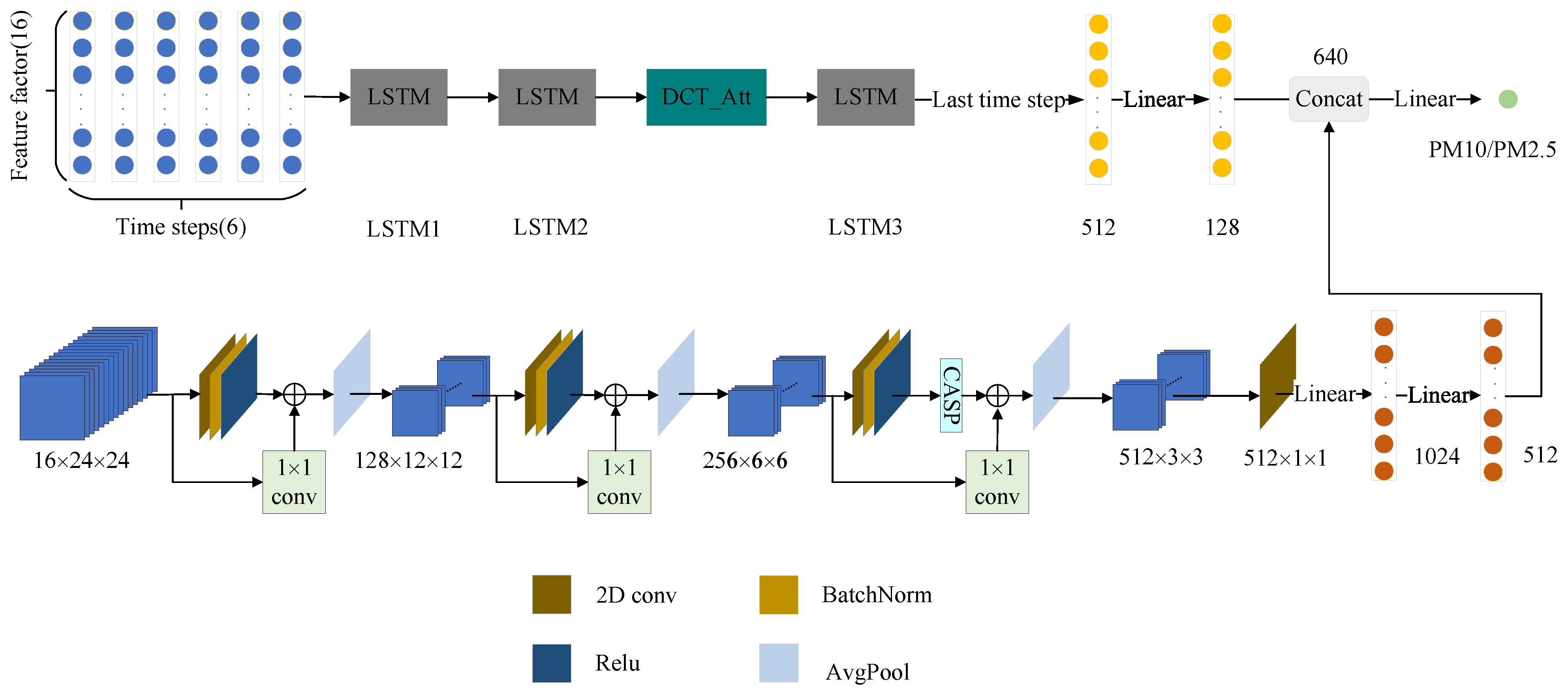
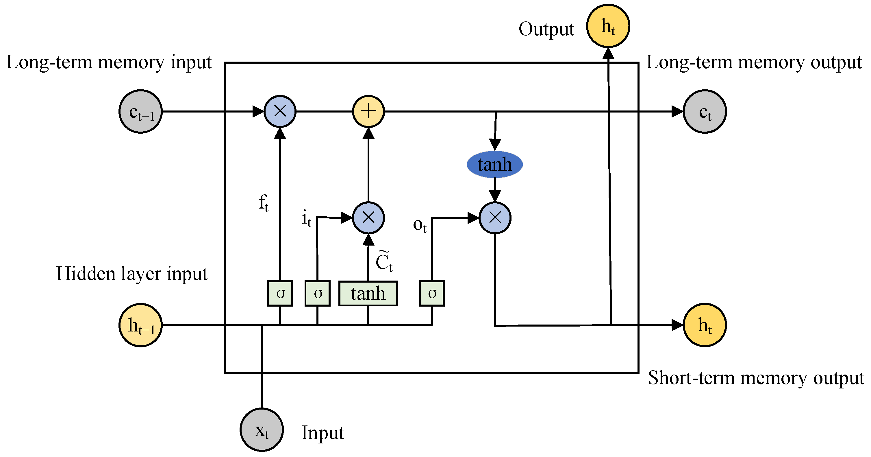
Currently, most models for particulate matter concentration retrieval primarily rely on traditional machine learning methods or neural networks that process one-dimensional data. In contrast, studies that construct multi-source data into two-dimensional images and utilize Convolutional Neural Networks (CNN) for retrieval remain relatively scarce. This paper fully combines the spatial feature extraction ability of CNN and the temporal feature extraction ability of LSTM, and proposes a CNN-LSTM dual-branch structure for the retrieval of particulate matter concentrations. The main contributions of this work are as follows:
(1) The dual-branch CNN-LSTM architecture proposed in this paper for particulate matter concentration inversion effectively integrates both spatial and temporal information, demonstrating superior performance in PM10 and PM2.5 retrieval compared to existing methods.
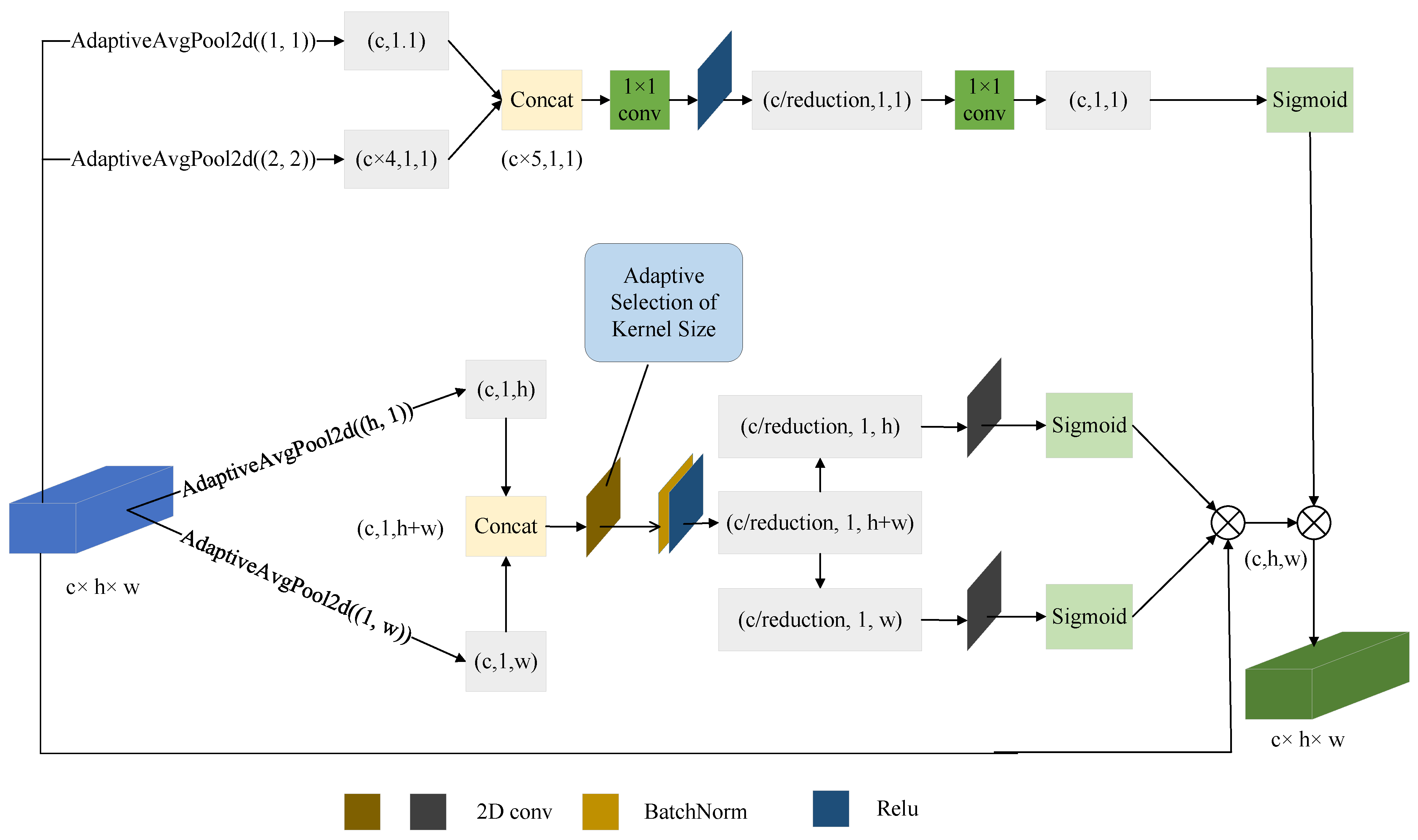
(2) To improve the inversion accuracy, we incorporated the Channel Attention (CASP) module into the CNN branch to enhance the extraction of channel features, and integrated the Temporal Attention (DCT_Att) module into the LSTM branch to strengthen the capture of temporal features.
The paper is organized as follows:
Section 1 begins by describing the dataset and preprocessing steps, and then provides a detailed explanation of the CSLTNet model’s architecture and working principles.
Section 2 discusses the experimental findings and analysis.
Section 3 discusses the findings and suggests potential directions for future improvements.
Section 4 summarizes the key contributions of this study.
3. Results
This study employs PyTorch 2.1.1 for all experiments, running on a Rocky Linux 8.10 (Green Obsidian) system with the following hardware: an INTEL XEON PLATINUM 8575C processor, 512 GB RAM, and an NVIDIA RTX 4090 GPU (24 GB VRAM). For CSLTNet training, we use the Adam optimizer with MSE loss, a learning rate of 1 × 10⁻⁴, and a batch size of 800.
To obtain quantitative evaluation results, this study employs correlation coefficient (
R), coefficient of determination (
R2), mean absolute error (MAE), root mean square error (RMSE), mean absolute percentage error (MAPE), and expected error (EE) as performance metrics. The coefficient
R quantifies the linear relationship between predicted and observed values;
R2 indicates the percentage of variance in the dependent variable accounted for by the regression model; MAE measures the mean absolute deviation between predictions and true values; RMSE computes the root mean square of prediction errors, exhibiting greater sensitivity to extreme values; MAPE expresses the average prediction error as a percentage, suitable for relative error assessment; a better EE value (closer to 100%) indicates higher consistency between estimated and actual values [
44].
The definitions of the six indicators are as follows:
where
denotes the predicted value, and
denotes the true value.
3.1. Ablation Experiment
In this section, we conducted ablation experiments on the modules in CSLTNet to evaluate the effectiveness of each module. All ablation experimental results were obtained based on the ten-fold cross-validation method.
3.1.1. Ablation Experiment on PM10
As shown in
Table 2, the combination of all modules yields the best results, and the fusion of dual branches performs better than a single branch.
3.1.2. Ablation Experiment on PM2.5
As shown in
Table 3, the combination of all modules yields the best results, and the fusion of dual branches performs better than a single branch.
3.2. Comparative Experiment
To verify the superiority of CSLTNet in the task of particulate matter concentration inversion, we compared it with four machine learning models and three deep learning models, including RF, XGBoost, CatBoost, LightGBM, Hybrid DL [
45], ResNet [
2], and CombineDeepNet [
46]. All comparative experiments of the aforementioned algorithms were conducted under the same experimental settings, based on sample-based 10-fold cross-validation and station-based 10-fold cross-validation.
3.2.1. Comparative Experiment on PM10
The 10-fold cross-validation results based on samples for different models in the PM
10 concentration inversion task are shown in
Table 4 and
Table 5. CSLTNet achieves the best performance in all metrics in both the Beijing–Tianjin–Hebei region and the Northwest region, including R, R
2, MAE, RMSE, MAPE (%) and withEE (%).
The 10-fold cross-validation results based on stations for different models in the PM
10 concentration inversion task are shown in
Table 6 and
Table 7. CSLTNet achieves the best performance across all metrics in both the Beijing–Tianjin–Hebei region and the Northwest region, including R, R
2, MAE, RMSE, MAPE (%), and withEE (%).
The experimental results demonstrate that CSLTNet, leveraging its dual-branch Convolutional Neural Network (CNN) and LSTM architecture, outperforms existing inversion networks in the PM10 concentration inversion task. Furthermore, the model exhibits stronger applicability in the northwestern region of China, where monitoring sites are sparsely distributed.
3.2.2. Comparative Experiment on PM2.5
The 10-fold cross-validation results based on samples for different models in the PM
2.5 concentration inversion task are shown in
Table 8 and
Table 9. CSLTNet achieves the best performance in all metrics in both the Beijing–Tianjin–Hebei region and the Northwest region, including R, R
2, MAE, RMSE, MAPE (%) and withEE (%).
The 10-fold cross-validation results based on stations for different models in the PM
2.5 concentration inversion task are shown in
Table 10 and
Table 11. CSLTNet achieves the best performance in all metrics in both the Beijing–Tianjin–Hebei region and the Northwest region, including R, R
2, MAE, RMSE, MAPE (%) and withEE (%).
The experimental results demonstrate that CSLTNet, leveraging its dual-branch Convolutional Neural Network (CNN) and LSTM architecture, outperforms existing inversion networks in the PM2.5 concentration inversion task. Furthermore, the model exhibits stronger applicability in the northwestern region of China, where monitoring sites are sparsely distributed.
3.2.3. Performance of Different Models on Unknown Region
To further evaluate the generalization ability of our proposed model, we conducted validation using sites in unknown regions. Specifically, the model was trained on data from the Beijing–Tianjin–Hebei region and tested using monitoring sites in Yinchuan, China. The information of the monitoring sites in Yinchuan is presented in
Table 12.
As shown in
Table 13 and
Table 14, the performance of our proposed model significantly outperforms other models in unknown regions, demonstrating its superior generalization capability.
3.3. Performance Across Different Seasons
Figure 9 and
Figure 10 demonstrate the seasonal performance of PM
10 concentration retrieval by the CSLTNet model in two regions. Overall, the PM
10 concentrations in Northwest China are significantly higher than those in the Beijing–Tianjin–Hebei region. The primary reason for this discrepancy is likely the frequent dust events occurring in the northwestern areas, which lead to substantial increases in particulate matter concentrations during such episodes. In the Beijing–Tianjin–Hebei region, the model demonstrated optimal performance during spring and the poorest performance in summer. Similarly, in Northwest China, the model also achieved its best performance in spring, while the weakest performance was observed in winter.
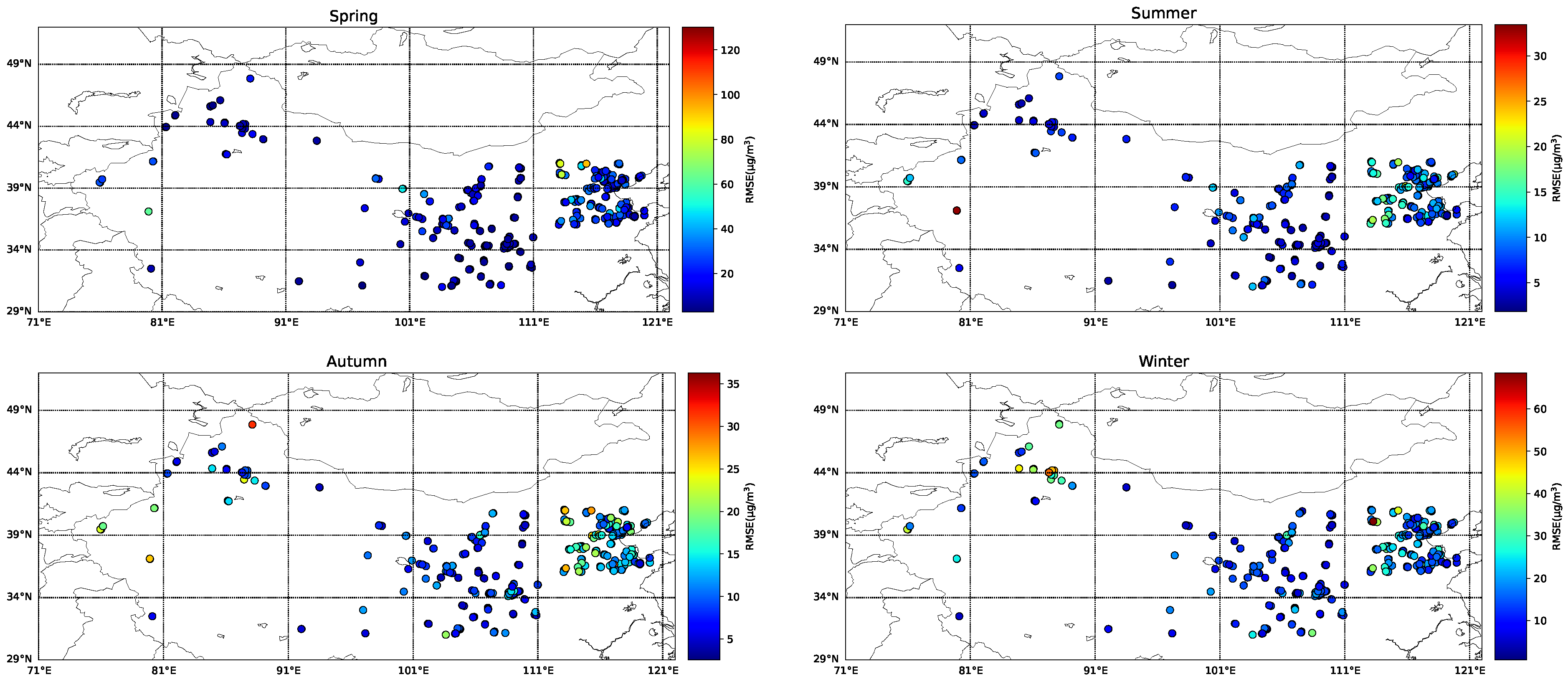
Figure 11 illustrates the spatial distribution characteristics of PM
10 model errors across different seasons. The model exhibits the highest error values in both major regions during spring, while errors are relatively lower in summer and autumn. Areas near deserts (such as northern Xinjiang) and regions along dust transport pathways (e.g., central Inner Mongolia) show relatively higher errors. This spatial pattern of error distribution is consistent with the results shown in the scatter plots.
Figure 12 and
Figure 13 demonstrate the seasonal performance of PM
2.5 concentration retrieval by the CSLTNet model in two regions. Overall, both regions exhibited the highest RMSE values during winter, which is likely attributable to extensive fossil fuel combustion for heating purposes in this season. In the Beijing–Tianjin–Hebei region, the model performed optimally in winter and least effectively in summer. In Northwest China, however, the model demonstrated relatively consistent performance across all four seasons with minimal seasonal variation.
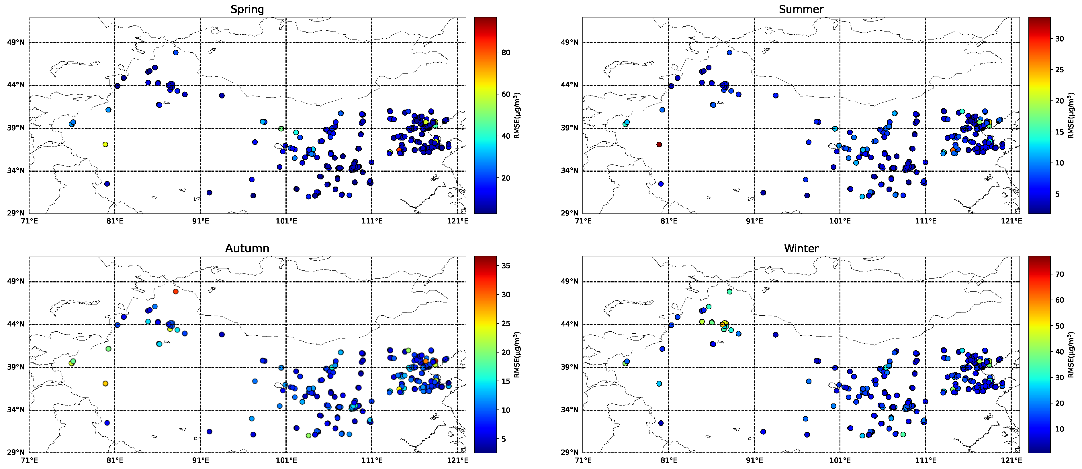
Figure 14 illustrates the spatial distribution of PM
2.5 model errors across different seasons. Relatively higher errors are observed in spring and winter, with the Northwest region exhibiting more pronounced errors than the Beijing–Tianjin–Hebei region. In contrast, errors during summer and autumn are lower, with minimal differences between the two regions. This spatial pattern of errors is consistent with the scatter plot results.
3.4. Spatial Distribution of Retrieval Results and Comparison of Model Performance Across Different Regions
As shown in
Figure 15 and
Figure 16, the spatial distribution of PM
10 and PM
2.5 exhibits strong continuity, with the model-predicted values highly consistent with the actual observed values.
As illustrated in
Figure 17, in both 2021 and 2022, certain areas in Northwest China (such as those near desert zones) displayed darker-colored points, indicating relatively higher errors. In desert regions, complex factors like dust weather significantly influence PM
10 concentrations, leading to comparatively larger model deviations. In contrast, urban areas within Northwest China exhibited relatively smaller model errors. The Beijing–Tianjin–Hebei region, being a densely urbanized area, involves complex sources of PM
10 emissions from industrial, transportation, and other human activities. For both 2021 and 2022, the data points in this region are predominantly blue, suggesting relatively lower errors. This implies that the model’s simulation error for PM
10 in the Beijing–Tianjin–Hebei region is relatively small, potentially due to the abundance of observational data and the more readily identifiable patterns of anthropogenic PM
10 emissions in this area.
As shown in
Figure 18, the spatial distribution of errors in PM
2.5 and PM
10 demonstrates consistency. The higher observation errors at some sites in the Beijing–Tianjin–Hebei region may be attributed to intensive industrial and traffic pollution emissions in this area.
Overall, the PM10 and PM2.5 models perform better with smaller errors in the Beijing–Tianjin–Hebei region—characterized by dense urbanization, significant human influence, and relatively abundant observational data. In contrast, these models show relatively larger errors and slightly inferior performance in Northwest China, where complex geographical conditions (such as desert belt influences, diverse underlying surfaces, and substantial interference from natural factors like dust) prevail.

