Highlights
What are the main findings?
- A dual-branch CNN-LSTM architecture that integrates spatial and temporal information was proposed for particulate matter concentration retrieval.
- The feature extraction capability is enhanced by introducing both channel attention and temporal attention mechanisms.
What is the implication of the main finding?
- Our study provides a robust solution for high-precision, large-scale air quality monitoring, particularly in data-sparse regions.
- Our inversion framework provides a reusable architectural strategy for other spatiotemporal sequence prediction tasks.
Abstract
The concentrations of atmospheric particulate matter (PM10 and PM2.5) significantly impact global environment, human health, and climate change. This study developed a particulate matter concentration retrieval method based on multi-source data, proposing a dual-branch retrieval network architecture named CSLTNet that integrates Convolutional Neural Networks (CNN) and Long Short-Term Memory (LSTM) networks. The CNN branch is designed to extract spatial features, while the LSTM branch captures temporal characteristics, with attention modules incorporated into both the CNN and LSTM branches to enhance feature extraction capabilities. Notably, the model demonstrates robust spatial generalization capability across different geographical regions.Comprehensive experimental evaluations demonstrate the outstanding performance of the CSLTNet model. For the Beijing–Tianjin–Hebei region in China: in PM10 retrieval, sample-based 10-fold cross-validation achieved R2 = 0.9427 (RMSE = ), while station-based validation yielded R2 = 0.9213 (RMSE = ); for PM2.5 retrieval, sample-based 10-fold cross-validation resulted in R2 = 0.9579 (RMSE = ), with station-based validation reaching R2 = 0.9296 (RMSE = ). For Northwest China: in PM10 retrieval, sample-based 10-fold cross-validation achieved R2 = 0.9236 (RMSE = ), while station-based validation yielded R2 = 0.9046 (RMSE = ); for PM2.5 retrieval, sample-based 10-fold cross-validation resulted in R2 = 0.9279 (RMSE = ), with station-based validation reaching R2 = 0.8787 (RMSE = ).
1. Introduction
In recent years, air pollution has emerged as a growing environmental concern. The acceleration of industrial development and urban expansion has significantly exacerbated this pressing issue. Particulate matter with an aerodynamic diameter of less than (PM2.5) [1,2] and particulate matter with an aerodynamic diameter of less than (PM10) [3,4] have a significant impact on the global environment, human health, and climate change. The increase in the concentrations of PM2.5 and PM10 will not only affect the local climate, but also increase the incidence and mortality rates of various diseases [5]. In 2019, the World Health Organization (WHO) reported that outdoor air pollution, affecting both cities and rural regions, was responsible for approximately 4.2 million premature deaths worldwide. This mortality was attributed to prolonged contact with fine particulate matter, known to increase risks of heart disease, lung disorders, and certain cancers. In addition, the pollution problems caused by PM2.5 and PM10 will also result in economic losses. They will not only reduce production efficiency but also increase the costs of pollution control measures, electricity consumption, coal usage, and other aspects [6]. The most direct method to obtain particulate matter concentration is through environmental monitoring stations. However, due to the uneven spatial distribution of ground monitoring stations, there is a lack of high-precision data that is continuous both in time and space [7]. This has limited the research on the climatic environment of atmospheric PM10 and PM2.5 [8,9].
Due to its extensive spatial coverage and high resolution, satellite remote sensing has been widely adopted as a key method for estimating particulate matter (PM) concentrations [10]. Research indicates a significant relationship between satellite-derived aerosol optical depth (AOD) measurements and ground-level particulate pollutants, including PM2.5 and PM10 [11,12,13].
The methods for retrieving particulate matter concentration can be broadly classified into three categories: physical or chemical methods [14], semi-empirical methods, and statistical methods. The semi-empirical model combines theoretical analysis with experimental data. The physical and chemical model is constructed based on an in-depth understanding of the physical and chemical processes of PM2.5, PM10, and aerosols. It takes into detailed consideration the physical and chemical mechanisms such as the formation, evolution, and transportation of aerosols, as well as their interactions with other components in the atmosphere. Based on a certain physical theory, it describes the characteristics of PM2.5 and PM10 by introducing some empirical parameters or relationships.
Statistical approaches avoid the need to account for intricate physical transformations, chemical interactions, or transport mechanisms [4]. Operating purely through pattern recognition between input features and response variables, these methods demonstrate markedly lower computational demands than competing techniques. Statistical model methods can be roughly divided into three categories: regression-based methods, machine learning methods, and hybrid model methods. The regression-based method, with the characteristics of clear principles and simple operation, is widely applied in the field of particulate matter concentration retrieval. Zaman et al. [15] constructed a Multiple Linear Regression (MLR) approach, achieving a Cross-Validation (CV) R2 of 0.66. You et al. [16] proposed a Generalized Additive Model (GAM) that demonstrated strong predictive performance, with daily-scale correlations (R) reaching 0.67 and seasonal-scale correlations varying between 0.7 and 0.9. Xiao et al. [17] proposed the LME-GAM model, which demonstrated strong predictive performance in China’s Yangtze River Delta region. The study reported 10-fold cross-validation results showing R2 values of 0.81 with an RMSE of for 2013 and 0.73 with an RMSE of for 2014.
Machine learning has demonstrated remarkable success in estimating pollutant concentrations, owing to its exceptional capacity for handling nonlinear relationships and performing parallel computations. Zamani et al. [18] employed RF, XGBoost, and deep learning methods to estimate PM2.5 concentrations in Tehran’s urban areas. The results demonstrated that the XGBoost model exhibited optimal performance, with a determination coefficient (R2) of 0.81 (correlation coefficient R = 0.90), mean absolute error (MAE) of , and root mean square error (RMSE) of . Chen et al. [19] proposed an ensemble machine learning framework integrating AdaBoost, XGBoost and Random Forest algorithms for PM2.5 concentration estimation across central and eastern China. Their stacking model demonstrated robust predictive accuracy, achieving mean R2 and RMSE values of 0.85 and , respectively. Wei et al. [12] developed a Spatio-Temporal Random Forest (STRF) model. Based on the sample-based ten-fold cross-validation, its coefficient of determination is 0.85, the root mean square error is , and the mean prediction error is . Chen et al. [20] employed a Deep Forest (DF) algorithm to establish a novel AOD-PM10 correlation model, integrating Aerosol Optical Depth with near-surface particulate matter concentrations. The model demonstrated strong temporal consistency, with determination coefficients (R2) of 0.87 (daily), 0.91 (monthly), 0.94 (seasonal), and 0.94 (annual) across different time scales. Tian et al. [21] applied an enhanced XGBoost algorithm for particulate matter concentration prediction. The model achieved high accuracy, with PM10 estimation showing R2 = 0.90 and RMSE = , while PM2.5 prediction yielded R2 = 0.89 and RMSE = . Xu et al. [22] proposed a stacking model (Stacking-BP-ET model) that incorporates a backpropagation neural network and extremely randomized trees, and constructed a global PM10 dataset with a spatial resolution of 1 km from 2015 to 2021. The coefficient of determination (R2) of the spatiotemporal cross-validation outside the stations and outside the years for this product is 0.833, and MAE and RMSE are and , respectively.
Neural networks possess the capability to autonomously adapt their parameters, allowing the output to progressively converge toward the desired target. Therefore, it is capable of handling most nonlinear problems. Wu et al. [23] developed a back-propagation artificial neural network (BPNN) trained with Bayesian regularization to estimate the PM mass concentration in eastern China. Li et al. [24] developed the Geoi-DBN framework, which incorporates geographical distance parameters into a deep belief network architecture for predicting ground-level PM2.5 concentrations. Their model achieved an out-of-sample cross-validation R2 value of 0.88, with a corresponding RMSE of . More and more researchers have found that it is difficult for a single statistical model to further explore the nonlinear relationship between particulate matter concentration and satellite remote sensing data. Therefore, a large number of hybrid models have been applied to the estimation of particulate matter concentration. Wu et al. [25] developed a hybrid deep learning model called BiCNN by combining CNN with BiLSTM networks to predict PM2.5 concentrations from AOD data. Their proposed model achieved superior performance in annual-scale predictions, with an explained variance (R2) of 0.836, while maintaining low error rates (RMSE = , MAPE = 12.497). Shtein et al. [26] employed an innovative ensemble technique that integrated multiple predictive models, including a linear mixed effects approach, a random forest algorithm, an extreme gradient boosting system, and the Flexible Air Quality Regional Model. This integration was accomplished through a Geographically Weighted Generalized Additive Model framework, which incorporated dynamic weighting coefficients that adjusted according to both geographic location and temporal factors. Their research findings indicated that this spatially and temporally adaptive ensemble methodology outperformed all constituent models when evaluated individually. Liu et al. [27] proposed an innovative approach that merges the random forest algorithm with kriging interpolation techniques. This hybrid methodology successfully incorporates surface-level PM2.5 monitoring data and relevant geographic parameters, while simultaneously addressing both nonlinear relationships and intricate spatial correlation patterns. Fu et al. [28] proposed a novel stacked ensemble approach called XGBLL, which integrates XGBoost and LightGBM as base learners in the first layer, followed by a linear regression meta-model in the second layer. Their experimental results demonstrated that this combined framework achieves higher predictive accuracy compared to individual standalone models. Zeng et al. [29] introduced a novel two-phase framework for reconstructing spatially continuous PM2.5 distributions. The initial phase employs LightGBM to generate complete daily AOD coverage, while the subsequent phase incorporates a graph neural network-based architecture (ST-GAT) to capture spatiotemporal patterns for PM2.5 prediction. This approach demonstrated strong predictive capability, yielding an R2 of 0.88 and RMSE of in validation tests.
Currently, most models for particulate matter concentration retrieval primarily rely on traditional machine learning methods or neural networks that process one-dimensional data. In contrast, studies that construct multi-source data into two-dimensional images and utilize Convolutional Neural Networks (CNN) for retrieval remain relatively scarce. This paper fully combines the spatial feature extraction ability of CNN and the temporal feature extraction ability of LSTM, and proposes a CNN-LSTM dual-branch structure for the retrieval of particulate matter concentrations. The main contributions of this work are as follows:
(1) The dual-branch CNN-LSTM architecture proposed in this paper for particulate matter concentration inversion effectively integrates both spatial and temporal information, demonstrating superior performance in PM10 and PM2.5 retrieval compared to existing methods.
(2) To improve the inversion accuracy, we incorporated the Channel Attention (CASP) module into the CNN branch to enhance the extraction of channel features, and integrated the Temporal Attention (DCT_Att) module into the LSTM branch to strengthen the capture of temporal features.
The paper is organized as follows: Section 1 begins by describing the dataset and preprocessing steps, and then provides a detailed explanation of the CSLTNet model’s architecture and working principles. Section 2 discusses the experimental findings and analysis. Section 3 discusses the findings and suggests potential directions for future improvements. Section 4 summarizes the key contributions of this study.
2. Materials and Methods
2.1. Materials
The data required for retrieval is shown in Table 1. It also includes relative humidity (RH) and wind direction data, which are calculated using Equations (1)–(3). In addition, the day of the year and the month are included as temporal information. The data required for inversion can be broadly classified into three categories: AOD data, site monitoring data, and auxiliary data. AOD data and auxiliary data serve as feature variables, while PM10 and PM2.5 act as target variables. The AOD data includes two data products from NASA satellites. The site monitoring data includes two types of data, PM10 and PM2.5. We selected two typical regions in China—the Beijing–Tianjin–Hebei region and Northwest China—as study areas. The distribution of monitoring sites is shown in Figure 1, with approximately 254 sites in the Beijing–Tianjin–Hebei region and about 275 sites in Northwest China. The auxiliary data includes 11 meteorological factors, 2 types of land-use data, and 2 temporal elements. Numerous studies indicate that these additional factors have a substantial impact on ground-level particulate matter concentrations [30,31,32,33,34].

Table 1.
Details of the data used in this study.
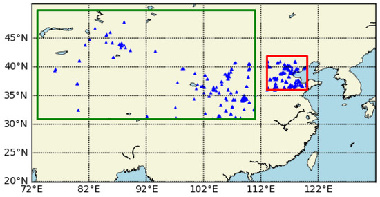
Figure 1.
Site distribution map. The green box represents the Northwest China region, the red box represents the Beijing-Tianjin-Hebei region, and the blue triangle denotes the monitoring stations.
2.2. Data Preprocessing
Data preprocessing mainly includes AOD filling, spatial resolution sampling, screening of abnormal values at monitoring sites, and spatiotemporal matching.
2.2.1. ERA5 Data Resolution Sampling
First, average the hourly ERA5 data to obtain daily data. Then, perform upsampling in the spatial domain. Then, use the bilinear interpolation method to upsample the spatial resolution to 1 km. As shown in Figure 2, for any point to be interpolated in the target high-resolution image, its position in the original low-resolution image may not exactly correspond to a known pixel point. Instead, it lies within a small rectangular area formed by four known pixel points , , and . The principle of bilinear interpolation is based on calculating the value of the point P to be interpolated through weighted averaging of the points within this small rectangular area. The specific steps are as follows:
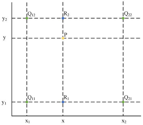
Figure 2.
Schematic diagram of bilinear interpolation.
First, on the line , linear interpolation is performed on point P in the x-direction to calculate the value of . According to the linear interpolation formula, the value of is
Similarly, on the line , linear interpolation is performed on point P in the x-direction to calculate the value of :
After obtaining and , linear interpolation is then performed on in the y-direction to obtain the value of :
In this way, for each point in the target high-resolution image, based on its relative position in the original low-resolution image, bilinear interpolation calculations can be carried out using the values of the four surrounding known pixel points. Thus, the attribute value of this point can be obtained. Eventually, a higher-resolution image is generated, achieving an improvement in spatial resolution. The schematic diagram of ERA5 data sampling is shown in Figure 3.
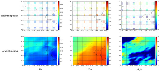
Figure 3.
Upsampling the spatial resolution of ERA5 data.
This study employed bilinear interpolation for the spatial upsampling of ERA5 reanalysis data, primarily based on the following two considerations. First, many meteorological variables provided by ERA5 (such as temperature and pressure) exhibit spatially continuous and smooth distribution characteristics. Under these conditions, bilinear interpolation maintains good accuracy with low computational cost, and this method has been successfully applied and validated in several previous relevant studies [2,3,20,35]. Second, the error introduced during the process of matching ERA5 data to the model’s input resolution via bilinear interpolation remains within an acceptable range when compared to other sources of uncertainty in the model itself.
2.2.2. Filling of Missing AOD Values
Due to the influence of high-brightness surfaces such as clouds and snow, as well as various human-related factors, there are a large number of missing values in the MCD19A2 data. To achieve seamless spatio-temporal retrieval of particulate matter concentration, filling the missing values of AOD is a necessary task. Methods for filling missing AOD values mainly include multi-source data fusion [12,36,37], spatial interpolation [15,38], multiple estimation [26,39], etc. In this study, filling of missing values was mainly carried out through multi-source data fusion. However, interpolation-based filling methods were also incorporated. The overall filling approach adopts a three-stage scheme. In the first stage, the MCD19A2 data is processed. Since MCD19A2 contains observations from both Terra and Aqua satellites, a complementary fusion method is applied to merge the AOD data from the two satellites to minimize information loss. The two satellites have different overpass times. If AOD data from both satellites are available, their average is taken as the final value; if only one satellite provides valid data, that value is directly used; if data from both satellites are missing, the gaps will be filled in the second processing stage. In the second stage, the MERRA-2 data is processed. First, the 24 h data is averaged to obtain daily data. Then, through bilinear interpolation, the spatial resolution is upsampled to 1 km. In the third stage, the sampled MERRA-2 data is filled into the missing positions of the MCD19A2 data processed in the first stage through the nearest-neighbor pixel matching method. Through the above steps, seamless spatiotemporal coverage of AOD is achieved. The schematic diagram of filling missing AOD values is shown in Figure 4.
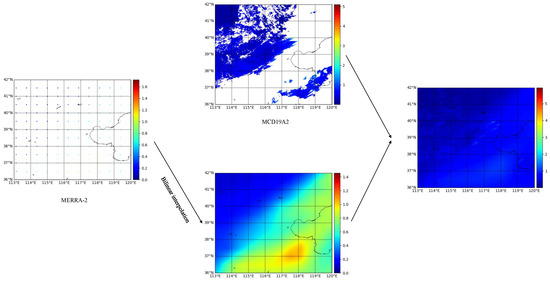
Figure 4.
Schematic diagram of AOD missing value filling.
We selected MERRA-2 data to fill the AOD gaps based on the following considerations. First, as a reanalysis product, MERRA-2 provides complete spatiotemporal coverage, which is essential for maintaining data continuity in the input to our deep learning model. Second, precedents exist demonstrating that using reanalysis data to compensate for AOD gaps is a validated and reliable strategy for ensuring data continuity and model stability [40,41]. Furthermore, to maintain consistency in data processing, we applied the same bilinear interpolation procedure to the MERRA-2 data as used for the meteorological factors. This approach not only ensures spatial consistency across all input data but also avoids introducing confounding errors that might arise from using different interpolation schemes. While we acknowledge that this may introduce some uncertainty, its impact on the retrieval of particulate matter concentrations remains within an acceptable range, especially when mitigated through synergistic use with other data sources and the error-correction mechanisms inherent in our model.
2.2.3. Screening of Outliers at Stations
In the hourly observational data of PM10 and PM2.5 at stations, there may be outliers caused by instrument malfunctions. To enable the model to fit better, it is necessary to filter out these outliers. In this study, the method of calculating the z-score is used to handle the outliers. Employ the z-score approach to filter out the outliers in the hourly monitoring data of each day. Subsequently, calculate the average of the valid hourly monitoring values to serve as the daily monitoring concentration value. After processing, the Beijing–Tianjin–Hebei region obtained a total of 144,489 valid PM10 station monitoring records and 144,501 valid PM2.5 station monitoring records in 2021 and 2022, while the Northwest region obtained 160,552 valid PM10 station monitoring records and 160,421 valid PM2.5 station monitoring records.
2.3. Network Architecture
The overall structure of CSLTNet is illustrated in Figure 5. It adopts a 1D-2D hybrid structure, consisting of two branches, namely the two-dimensional branch and the one-dimensional branch. The two-dimensional branch uses a CNN as the backbone network, and the one-dimensional branch uses an LSTM as the backbone network. The CNN branch is used to extract spatial information, and the LSTM branch is used to extract temporal information. Finally, the results of the two branches are fused together to implement the spatio-temporal hybrid dual-branch inversion network, CSLTNet.
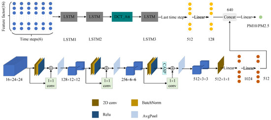
Figure 5.
The overall structure of CSLTNet.
In the CNN branch, given an input image , the resolution is , and it has 16 channels. These 16 channels represent 16 distinct feature factors, respectively. The convolutional layer, normalization layer, ReLU (Rectified Linear Unit), and average pooling layer are treated as a set of processing units. Here, the convolutional kernel size is , the padding is , the average pooling window size is , and the stride of the window moving over the input feature map is . After three processing steps, the resulting feature map sizes are , , and , respectively. In each layer, the dimensionality is adjusted using convolutions before the convolutional layer and after the ReLU layer, introducing residual connections. Additionally, an attention mechanism is incorporated between the third ReLU layer and the average pooling layer. For the feature map, it is flattened into one dimension using a convolution with a stride of 3. Finally, the output of the CNN branch is obtained by passing through two fully connected layers.
In the LSTM branch, the input feature map has a size of . Here, 6 represents the six time steps, including the current day and the previous five days, while 16 represents the 16 different feature factors (the LSTM branch only extracts features from the center pixel). A temporal attention mechanism, DCT_Att, is incorporated between the second and third layers. After processing through three LSTM layers (with the hidden layer size set to 512), the output of the last time step is taken to obtain one-dimensional features. These features are then processed through a fully connected layer to produce the final output of the LSTM branch.
The setting of the CNN and LSTM window sizes was determined based on extensive preliminary experimentation. The determination of the CNN window size aimed to balance the “receptive field” and “computational efficiency”. A 24 × 24 pixel area is sufficient to cover the spatial range centered on the target site that can exert an influence on it, while avoiding the introduction of excessive irrelevant noise and computational burden from an overly large network. Next, the LSTM window is explained. The determination of the LSTM window size was based on an analysis of the temporal dependency characteristics of particulate matter concentration and its influencing factors. The configuration of the current day and the previous five days (a total of 6 time steps) provides sufficient historical information to influence the current concentration, while avoiding the introduction of noise or excessive model training complexity due to overly long sequences.
The outputs of the two branches are merged via channel-wise concatenation and subsequently fed into a fully connected layer to predict the particulate matter concentration.
2.4. CNN Branch
2.4.1. Convolution and Pooling
The convolutional layer is a core module in this study. The size of the input image is , and the number of channels is 16. Sixteen channels represent sixteen different input factors. The convolution operation is equivalent to performing a “filter operation”. It multiplies each element of the convolution sum with a movable data window containing specific weights in the image and then sums them up, so as to achieve the extraction of image feature information. For the convolution process where the input is a feature map with a size of and the output is , the parameter relationships between the input layer and the output layer are:
Among them, k denotes the number of convolution kernels, s indicates the stride, p represents the padding, and the size of the convolution kernel is .
During convolution, the input feature map’s data window undergoes element-wise multiplication with the convolution kernel, followed by summation of these products to generate the output feature map. Typically, the output feature map has a smaller spatial dimension than the input due to the sliding window’s stride and the absence of padding. To maintain identical input and output dimensions, zero-padding can be applied to the input before convolution.
Pooling layers are typically applied following convolutional layers, employing downsampling to reduce feature map dimensions. This compression not only decreases computational complexity but also helps filter out less relevant features while mitigating overfitting. Two prevalent pooling methods in deep learning are max pooling and average pooling. For this research, average pooling was selected, which computes the mean of all activations within each pooling window as the output representation.
2.4.2. ReLU Activation Layer
In this study, the ReLU, that is, the Rectified Linear Unit, is used as the activation function. The mathematical expression of ReLU is shown in Equation (10).
2.4.3. Z-Score Normalization
The formula for Z-score normalization is shown in Equation (11). Here, X is the original data, is the mean of the data, is the standard deviation of the data, and Z is the standardized data.
The specific approach of this study is to standardize each feature individually.
2.4.4. CASP Attention Module
The overall structure of CASP attention is shown in Figure 6. CASP attention is fundamentally a dual-path hybrid attention network. The upper branch first performs two types of adaptive average pooling ( and ) on the input feature map, then concatenates the two pooling results. Subsequently, it computes channel attention weights through two convolutional layers (with ReLU activation in between), and finally normalizes the weights to the [0, 1] range using a Sigmoid function. The lower branch employs coordinate attention (CA) [42] with adaptive convolutional kernels [43]. It first conducts adaptive average pooling along the height and width directions separately, then dynamically determines the convolutional kernel size based on the number of input channels, followed by processing attention weights for the height and width directions independently. Ultimately, the attention feature map generated by CASP is the result of fusing the attention weights from both branches.
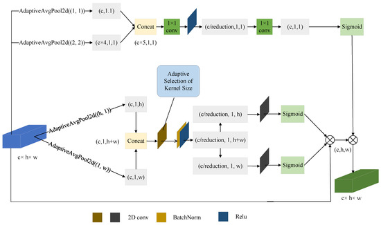
Figure 6.
The overall structure of CASP.
The kernel size k can be adaptively determined by Equation (12) given the channel dimension C.In this work, denotes the odd integer closest to t. For our experiments, we set the parameters and .
2.5. LSTM Branch
2.5.1. LSTM
The overall structure of LSTM is shown in Figure 7. The LSTM architecture includes several key components: a memory unit, a forgetting mechanism, a data entry mechanism, and a result generation mechanism. At its core lies the memory unit, which serves as the fundamental component for information flow throughout the sequence. This unit maintains extended temporal information while regulating data addition or elimination through specialized control mechanisms.
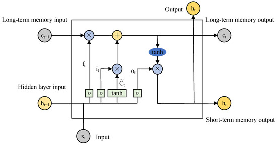
Figure 7.
The overall structure of LSTM.
The forgetting mechanism functions to identify and eliminate unnecessary data from the memory unit. By employing a sigmoid activation, it produces a numerical output ranging from 0 to 1, where 0 signifies total elimination and 1 indicates complete preservation.
The data entry mechanism governs the storage of new information within the memory unit. This process involves two operations: a sigmoid activation that selects which elements to modify, and a tanh activation that creates potential new values for updates.
Lastly, the result generation mechanism regulates the transfer of information from the memory unit to the current time step’s hidden representation. A sigmoid operation first filters the content to be transmitted, followed by a tanh transformation of the memory unit’s state to produce the final output.
2.5.2. DCT_Att Module
The overall structure of DCT_Att is shown in Figure 8. First, the input signal is transformed from the time domain to the frequency domain using the Discrete Cosine Transform (DCT-II). The DCT transform effectively captures periodic patterns and global dependencies in the sequence by decomposing the input sequence into cosine components of different frequencies. In the specific implementation, the Fast Fourier Transform (FFT) is employed to accelerate the computation: the input sequence is rearranged by concatenating the even-indexed elements and the reversed odd-indexed elements, followed by a real-valued FFT calculation. Finally, the DCT coefficients are obtained using cosine and sine weight matrices. For attention weight generation, after applying the DCT transform to the temporal features of each channel, Layer Normalization (LayerNorm) is used to stabilize the training process. The normalized features are then fed into a gating mechanism composed of a two-layer fully connected network. This network first expands the channel dimension by a factor of two, applies a ReLU activation function and Dropout regularization, and then compresses it back to the original channel dimension. The final attention weights, ranging between 0 and 1, are generated through a Sigmoid function. This structure enables the learning of nonlinear interactions between channels and emphasizes the role of important frequency components. Finally, the generated frequency-domain attention weights are multiplied channel-wise with the original input features to achieve feature recalibration.
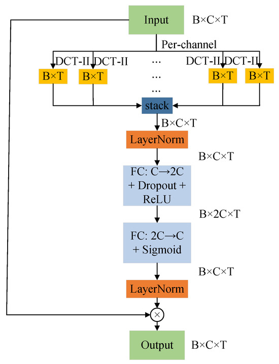
Figure 8.
The overall structure of DCT_Att.
3. Results
This study employs PyTorch 2.1.1 for all experiments, running on a Rocky Linux 8.10 (Green Obsidian) system with the following hardware: an INTEL XEON PLATINUM 8575C processor, 512 GB RAM, and an NVIDIA RTX 4090 GPU (24 GB VRAM). For CSLTNet training, we use the Adam optimizer with MSE loss, a learning rate of 1 × 10⁻⁴, and a batch size of 800.
To obtain quantitative evaluation results, this study employs correlation coefficient (R), coefficient of determination (R2), mean absolute error (MAE), root mean square error (RMSE), mean absolute percentage error (MAPE), and expected error (EE) as performance metrics. The coefficient R quantifies the linear relationship between predicted and observed values; R2 indicates the percentage of variance in the dependent variable accounted for by the regression model; MAE measures the mean absolute deviation between predictions and true values; RMSE computes the root mean square of prediction errors, exhibiting greater sensitivity to extreme values; MAPE expresses the average prediction error as a percentage, suitable for relative error assessment; a better EE value (closer to 100%) indicates higher consistency between estimated and actual values [44].
The definitions of the six indicators are as follows:
where denotes the predicted value, and denotes the true value.
3.1. Ablation Experiment
In this section, we conducted ablation experiments on the modules in CSLTNet to evaluate the effectiveness of each module. All ablation experimental results were obtained based on the ten-fold cross-validation method.
3.1.1. Ablation Experiment on PM10
As shown in Table 2, the combination of all modules yields the best results, and the fusion of dual branches performs better than a single branch.
Table 2.
Ablation experiment on module (PM10).
3.1.2. Ablation Experiment on PM2.5
As shown in Table 3, the combination of all modules yields the best results, and the fusion of dual branches performs better than a single branch.
Table 3.
Ablation experiment on module (PM2.5).
3.2. Comparative Experiment
To verify the superiority of CSLTNet in the task of particulate matter concentration inversion, we compared it with four machine learning models and three deep learning models, including RF, XGBoost, CatBoost, LightGBM, Hybrid DL [45], ResNet [2], and CombineDeepNet [46]. All comparative experiments of the aforementioned algorithms were conducted under the same experimental settings, based on sample-based 10-fold cross-validation and station-based 10-fold cross-validation.
3.2.1. Comparative Experiment on PM10
The 10-fold cross-validation results based on samples for different models in the PM10 concentration inversion task are shown in Table 4 and Table 5. CSLTNet achieves the best performance in all metrics in both the Beijing–Tianjin–Hebei region and the Northwest region, including R, R2, MAE, RMSE, MAPE (%) and withEE (%).
Table 4.
10-fold cross-validation results of different models on PM10 datasets from Beijing–Tianjin–Hebei region (sample-based split).
Table 5.
10-fold cross-validation results of different models on PM10 datasets from Northwest China (sample-based split).
The 10-fold cross-validation results based on stations for different models in the PM10 concentration inversion task are shown in Table 6 and Table 7. CSLTNet achieves the best performance across all metrics in both the Beijing–Tianjin–Hebei region and the Northwest region, including R, R2, MAE, RMSE, MAPE (%), and withEE (%).
Table 6.
10-fold cross-validation results of different models on PM10 datasets from Beijing–Tianjin–Hebei region (station-based split).
Table 7.
10-fold cross-validation results of different models on PM10 datasets from Northwest China (station-based split).
The experimental results demonstrate that CSLTNet, leveraging its dual-branch Convolutional Neural Network (CNN) and LSTM architecture, outperforms existing inversion networks in the PM10 concentration inversion task. Furthermore, the model exhibits stronger applicability in the northwestern region of China, where monitoring sites are sparsely distributed.
3.2.2. Comparative Experiment on PM2.5
The 10-fold cross-validation results based on samples for different models in the PM2.5 concentration inversion task are shown in Table 8 and Table 9. CSLTNet achieves the best performance in all metrics in both the Beijing–Tianjin–Hebei region and the Northwest region, including R, R2, MAE, RMSE, MAPE (%) and withEE (%).
Table 8.
10-fold cross-validation results of different models on PM2.5 datasets from Beijing–Tianjin–Hebei region (sample-based split).
Table 9.
10-fold cross-validation results of different models on PM2.5 datasets from Northwest China (sample-based split).
The 10-fold cross-validation results based on stations for different models in the PM2.5 concentration inversion task are shown in Table 10 and Table 11. CSLTNet achieves the best performance in all metrics in both the Beijing–Tianjin–Hebei region and the Northwest region, including R, R2, MAE, RMSE, MAPE (%) and withEE (%).
Table 10.
10-fold cross-validation results of different models on PM2.5 datasets from Beijing–Tianjin–Hebei region (station-based split).
Table 11.
10-fold cross-validation results of different models on PM2.5 datasets from Northwest China (station-based split).
The experimental results demonstrate that CSLTNet, leveraging its dual-branch Convolutional Neural Network (CNN) and LSTM architecture, outperforms existing inversion networks in the PM2.5 concentration inversion task. Furthermore, the model exhibits stronger applicability in the northwestern region of China, where monitoring sites are sparsely distributed.
3.2.3. Performance of Different Models on Unknown Region
To further evaluate the generalization ability of our proposed model, we conducted validation using sites in unknown regions. Specifically, the model was trained on data from the Beijing–Tianjin–Hebei region and tested using monitoring sites in Yinchuan, China. The information of the monitoring sites in Yinchuan is presented in Table 12.
Table 12.
Distribution information of sites in the verification region.
As shown in Table 13 and Table 14, the performance of our proposed model significantly outperforms other models in unknown regions, demonstrating its superior generalization capability.
Table 13.
Results of different models on PM2.5 datasets on unknown region.
Table 14.
Results of different models on PM10 datasets on unknown regions.
3.3. Performance Across Different Seasons
Figure 9 and Figure 10 demonstrate the seasonal performance of PM10 concentration retrieval by the CSLTNet model in two regions. Overall, the PM10 concentrations in Northwest China are significantly higher than those in the Beijing–Tianjin–Hebei region. The primary reason for this discrepancy is likely the frequent dust events occurring in the northwestern areas, which lead to substantial increases in particulate matter concentrations during such episodes. In the Beijing–Tianjin–Hebei region, the model demonstrated optimal performance during spring and the poorest performance in summer. Similarly, in Northwest China, the model also achieved its best performance in spring, while the weakest performance was observed in winter. Figure 11 illustrates the spatial distribution characteristics of PM10 model errors across different seasons. The model exhibits the highest error values in both major regions during spring, while errors are relatively lower in summer and autumn. Areas near deserts (such as northern Xinjiang) and regions along dust transport pathways (e.g., central Inner Mongolia) show relatively higher errors. This spatial pattern of error distribution is consistent with the results shown in the scatter plots.
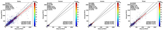
Figure 9.
Seasonal PM10 results from station-based cross-validation in the Beijing–Tianjin–Hebei region.
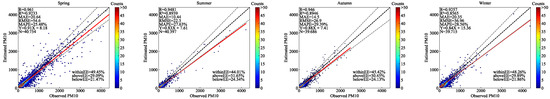
Figure 10.
Seasonal PM10 results from station-based cross-validation in Northwest China.
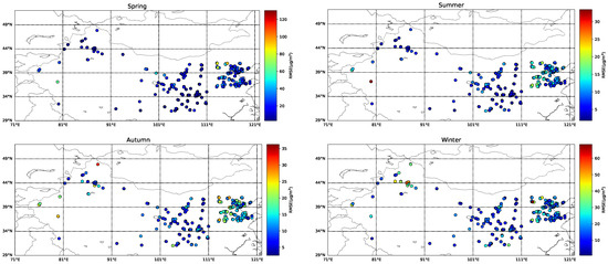
Figure 11.
Spatial Distribution of PM10 Model Errors by Season.
Figure 12 and Figure 13 demonstrate the seasonal performance of PM2.5 concentration retrieval by the CSLTNet model in two regions. Overall, both regions exhibited the highest RMSE values during winter, which is likely attributable to extensive fossil fuel combustion for heating purposes in this season. In the Beijing–Tianjin–Hebei region, the model performed optimally in winter and least effectively in summer. In Northwest China, however, the model demonstrated relatively consistent performance across all four seasons with minimal seasonal variation. Figure 14 illustrates the spatial distribution of PM2.5 model errors across different seasons. Relatively higher errors are observed in spring and winter, with the Northwest region exhibiting more pronounced errors than the Beijing–Tianjin–Hebei region. In contrast, errors during summer and autumn are lower, with minimal differences between the two regions. This spatial pattern of errors is consistent with the scatter plot results.
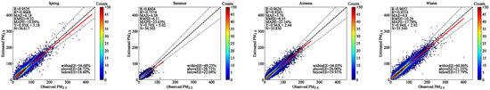
Figure 12.
Seasonal PM2.5 results from station-based cross-validation in the Beijing–Tianjin–Hebei region.
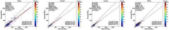
Figure 13.
Seasonal PM2.5 results from station-based cross-validation in Northwest China.
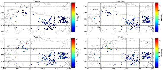
Figure 14.
Spatial Distribution of PM2.5 Model Errors by Season.
3.4. Spatial Distribution of Retrieval Results and Comparison of Model Performance Across Different Regions
As shown in Figure 15 and Figure 16, the spatial distribution of PM10 and PM2.5 exhibits strong continuity, with the model-predicted values highly consistent with the actual observed values.
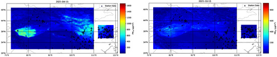
Figure 15.
Spatial Distribution of Retrieved PM10 Concentrations.
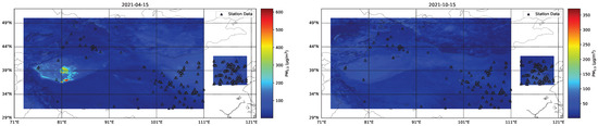
Figure 16.
Spatial Distribution of Retrieved PM2.5 Concentrations.
As illustrated in Figure 17, in both 2021 and 2022, certain areas in Northwest China (such as those near desert zones) displayed darker-colored points, indicating relatively higher errors. In desert regions, complex factors like dust weather significantly influence PM10 concentrations, leading to comparatively larger model deviations. In contrast, urban areas within Northwest China exhibited relatively smaller model errors. The Beijing–Tianjin–Hebei region, being a densely urbanized area, involves complex sources of PM10 emissions from industrial, transportation, and other human activities. For both 2021 and 2022, the data points in this region are predominantly blue, suggesting relatively lower errors. This implies that the model’s simulation error for PM10 in the Beijing–Tianjin–Hebei region is relatively small, potentially due to the abundance of observational data and the more readily identifiable patterns of anthropogenic PM10 emissions in this area.
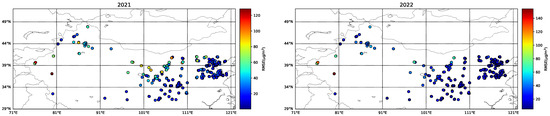
Figure 17.
Spatial Distribution Map of PM10 Model Errors.
As shown in Figure 18, the spatial distribution of errors in PM2.5 and PM10 demonstrates consistency. The higher observation errors at some sites in the Beijing–Tianjin–Hebei region may be attributed to intensive industrial and traffic pollution emissions in this area.
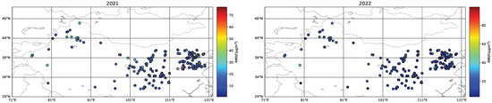
Figure 18.
Spatial Distribution Map of PM2.5 Model Errors.
Overall, the PM10 and PM2.5 models perform better with smaller errors in the Beijing–Tianjin–Hebei region—characterized by dense urbanization, significant human influence, and relatively abundant observational data. In contrast, these models show relatively larger errors and slightly inferior performance in Northwest China, where complex geographical conditions (such as desert belt influences, diverse underlying surfaces, and substantial interference from natural factors like dust) prevail.
4. Discussion
While the proposed model demonstrates strong performance in particulate concentration inversion, some limitations remain: The current architecture incorporates channel attention and temporal attention mechanisms but lacks spatial attention modules to further enhance feature extraction. Compared to machine learning models and one-dimensional deep learning models, the proposed architecture exhibits higher complexity. Future research will focus on developing spatial attention modules to improve feature representation and implementing measures to reduce model complexity. Additionally, follow-up studies will focus on constructing three-dimensional datasets and employing three-dimensional deep learning models to accomplish inversion tasks. It is also worth emphasizing that extending the current retrieval framework to temporal prediction will be an important direction for our future research.
5. Conclusions
This study establishes the Beijing–Tianjin–Hebei region and Northwest China as target areas, developing a specialized dataset for particulate matter concentration retrieval. To enhance retrieval performance, we propose a parallel dual-branch network integrating CNN and LSTM architectures. The framework simultaneously extracts spatial and temporal features through its dual pathways, with subsequent feature fusion generating more comprehensive and refined representations to significantly improve model accuracy. Through multi-angle experimental validation, CSLTNet has been proven an effective method for particulate matter concentration retrieval. The model demonstrated robust spatial generalizability and proved adaptable to concentration estimation across diverse geographical environments. Especially in Northwest China, where monitoring stations are sparsely distributed and there are significant variations between high and low concentration values, our model demonstrates superior adaptability.
Author Contributions
L.Y., software, methodology, and writing—original draft. Z.W., conceptualization, methodology, supervision, and writing—review and editing. Y.Z., visualization, investigation, and funding acquisition. All authors have read and agreed to the published version of the manuscript.
Funding
This work was supported by National Key Research and Development Program (2022YFF0711702) and the Fundamental Research Funds for the Central Universities (lzujbky-2024-it54).
Informed Consent Statement
Informed consent was obtained from all subjects involved in the study.
Data Availability Statement
PM10 and PM2.5 station observations in Chinese are available at http://www.cnemc.cn/. MERRA-2 AOD data are available from the MERRA-2 dataset at https://gmao.gsfc.nasa.gov/reanalysis/MERRA-2/ (accessed on 20 April 2025). ERA5 dataset is available at http://cds.climate.copernicus.eu/ (accessed on 20 April 2025). MCD19A2, MOD13A3 and MCD12Q1 datasets are available at https://ladsweb.modaps.eosdis.nasa.gov/ (accessed on 20 April 2025).
Conflicts of Interest
The authors declare that they have no known competing financial interests or personal relationships that could have appeared to influence the work reported in this paper.
References
- Bai, H.; Zheng, Z.; Zhang, Y.; Huang, H.; Wang, L. Comparison of satellite-based PM2.5 estimation from aerosol optical depth and top-of-atmosphere reflectance. Aerosol Air Qual. Res. 2021, 21, 200257. [Google Scholar] [CrossRef]
- Yin, S.; Li, T.; Cheng, X.; Wu, J. Remote sensing estimation of surface PM2.5 concentrations using a deep learning model improved by data augmentation and a particle size constraint. Atmos. Environ. 2022, 287, 119282. [Google Scholar] [CrossRef]
- Chen, B.; Song, Z.; Huang, J.; Zhang, P.; Hu, X.; Zhang, X.; Guan, X.; Ge, J.; Zhou, X. Estimation of atmospheric PM10 concentration in china using an interpretable deep learning model and top-of-the-atmosphere reflectance data from china’s new generation geostationary meteorological satellite, fy-4a. J. Geophys. Res. Atmos. 2022, 127, e2021JD036393. [Google Scholar] [CrossRef]
- Zhang, K.; Yang, X.; Cao, H.; Thé, J.; Tan, Z.; Yu, H. Multi-step forecast of PM2.5 and PM10 concentrations using convolutional neural network integrated with spatial–temporal attention and residual learning. Environ. Int. 2023, 171, 107691. [Google Scholar] [CrossRef]
- Renard, J.-B.; Surcin, J.; Annesi-Maesano, I.; Delaunay, G.; Poincelet, E.; Dixsaut, G. Relation between PM2.5 pollution and covid-19 mortality in western europe for the 2020–2022 period. Sci. Total Environ. 2022, 848, 157579. [Google Scholar] [CrossRef] [PubMed]
- Zhang, L.; Yang, G.; Li, X. Mining sequential patterns of PM2.5 pollution between 338 cities in china. J. Environ. Manag. 2020, 262, 110341. [Google Scholar] [CrossRef]
- Yan, X.; Zang, Z.; Luo, N.; Jiang, Y.; Li, Z. New interpretable deep learning model to monitor real-time PM2.5 concentrations from satellite data. Environ. Int. 2020, 144, 106060. [Google Scholar] [CrossRef]
- Yan, X.; Zang, Z.; Jiang, Y.; Shi, W.; Guo, Y.; Li, D.; Zhao, C.; Husi, L. A spatial-temporal interpretable deep learning model for improving interpretability and predictive accuracy of satellite-based PM2.5. Environ. Pollut. 2021, 273, 116459. [Google Scholar] [CrossRef] [PubMed]
- Zhang, Y.; Li, Z. Remote sensing of atmospheric fine particulate matter (PM2.5) mass concentration near the ground from satellite observation. Remote Sens. Environ. 2015, 160, 252–262. [Google Scholar] [CrossRef]
- Van Donkelaar, A.; Martin, R.V.; Brauer, M.; Hsu, N.C.; Kahn, R.A.; Levy, R.C.; Sayer, A.M.; Winker, D.M. Global estimates of fine particulate matter using a combined geophysical-statistical method with information from satellites, models, and monitors. Environ. Sci. Technol. 2016, 50, 3762–3772. [Google Scholar] [CrossRef]
- Xiao, L.; Lang, Y.; Christakos, G. High-resolution spatiotemporal mapping of PM2.5 concentrations at mainland china using a combined bme-gwr technique. Atmos. Environ. 2018, 173, 295–305. [Google Scholar] [CrossRef]
- Wei, J.; Huang, W.; Li, Z.; Xue, W.; Peng, Y.; Sun, L.; Cribb, M. Estimating 1-km-resolution PM2.5 concentrations across china using the space-time random forest approach. Remote Sens. Environ. 2019, 231, 111221. [Google Scholar] [CrossRef]
- Xu, Q.; Chen, X.; Yang, S.; Tang, L.; Dong, J. Spatiotemporal relationship between himawari-8 hourly columnar aerosol optical depth (aod) and ground-level PM2.5 mass concentration in mainland china. Sci. Total Environ. 2021, 765, 144241. [Google Scholar] [CrossRef]
- Li, Z.; Zhang, Y.; Shao, J.; Li, B.; Hong, J.; Liu, D.; Li, D.; Wei, P.; Li, W.; Li, L.; et al. Remote sensing of atmospheric particulate mass of dry PM2.5 near the ground: Method validation using ground-based measurements. Remote Sens. Environ. 2016, 173, 59–68. [Google Scholar] [CrossRef]
- Zaman, N.A.F.K.; Kanniah, K.D.; Kaskaoutis, D.G. Estimating particulate matter using satellite based aerosol optical depth and meteorological variables in malaysia. Atmos. Res. 2017, 193, 142–162. [Google Scholar] [CrossRef]
- You, W.; Zang, Z.; Pan, X.; Zhang, L.; Chen, D. Estimating PM2.5 in xi’an, china using aerosol optical depth: A comparison between the modis and misr retrieval models. Sci. Total Environ. 2015, 505, 1156–1165. [Google Scholar] [CrossRef] [PubMed]
- Xiao, Q.; Wang, Y.; Chang, H.H.; Meng, X.; Geng, G.; Lyapustin, A.; Liu, Y. Full-coverage high-resolution daily PM2.5 estimation using maiac aod in the yangtze river delta of china. Remote Sens. Environ. 2017, 199, 437–446. [Google Scholar] [CrossRef]
- Joharestani, M.Z.; Cao, C.; Ni, X.; Bashir, B.; Talebiesfandarani, S. PM2.5 prediction based on random forest, xgboost, and deep learning using multisource remote sensing data. Atmosphere 2019, 10, 373. [Google Scholar] [CrossRef]
- Chen, J.; Yin, J.; Zang, L.; Zhang, T.; Zhao, M. Stacking machine learning model for estimating hourly PM2.5 in china based on himawari 8 aerosol optical depth data. Sci. Total Environ. 2019, 697, 134021. [Google Scholar] [CrossRef]
- Chen, B.; Song, Z.; Shi, B.; Li, M. An interpretable deep forest model for estimating hourly PM10 concentration in china using himawari-8 data. Atmos. Environ. 2022, 268, 118827. [Google Scholar] [CrossRef]
- Tian, L.; Chen, L.; Zhang, P.; Hu, B.; Gao, Y.; Si, Y. The ground-level particulate matter concentration estimation based on the new generation of fengyun geostationary meteorological satellite. Remote Sens. 2023, 15, 1459. [Google Scholar] [CrossRef]
- Xu, X.; Chen, M.; Shen, J. Estimation of global ground-level PM10 concentrations using a stacking model. Int. J. Digit. Earth 2024, 17, 2385071. [Google Scholar] [CrossRef]
- Wu, Y.; Guo, J.; Zhang, X.; Tian, X.; Zhang, J.; Wang, Y.; Duan, J.; Li, X. Synergy of satellite and ground based observations in estimation of particulate matter in eastern china. Sci. Total Environ. 2012, 433, 20–30. [Google Scholar] [CrossRef]
- Li, T.; Shen, H.; Yuan, Q.; Zhang, X.; Zhang, L. Estimating ground-level pm2. 5 by fusing satellite and station observations: A geo-intelligent deep learning approach. Geophys. Res. Lett. 2017, 44, 11–985. [Google Scholar] [CrossRef]
- Wu, S.; Li, H.; Zhou, Y.; He, Y. PM2.5 estimation and analysis of bicnn model considering spatiotemporal characteristics: A case study of the middle reaches of the yangtze river urban agglomeration. Theor. Appl. Climatol. 2024, 155, 2787–2799. [Google Scholar] [CrossRef]
- Shtein, A.; Kloog, I.; Schwartz, J.; Silibello, C.; Michelozzi, P.; Gariazzo, C.; Viegi, G.; Forastiere, F.; Karnieli, A.; Just, A.C.; et al. Estimating daily PM2.5 and PM10 over italy using an ensemble model. Environ. Sci. Technol. 2019, 54, 120–128. [Google Scholar] [CrossRef]
- Liu, Y.; Cao, G.; Zhao, N.; Mulligan, K.; Ye, X. Improve ground-level PM2.5 concentration mapping using a random forests-based geostatistical approach. Environ. Pollut. 2018, 235, 272–282. [Google Scholar] [CrossRef]
- Fu, Q.; Guo, H.; Gu, X.; Li, J.; Zhang, W.; Mi, X.; Zhao, Q.; Chen, D. High-resolution PM2.5 concentrations estimation based on stacked ensemble learning model using multi-source satellite toa data. Remote Sens. 2023, 15, 5489. [Google Scholar] [CrossRef]
- Zeng, Q.; Li, Y.; Tao, J.; Fan, M.; Chen, L.; Wang, L.; Wang, Y. Full-coverage estimation of PM2.5 in the beijing-tianjin-hebei region by using a two-stage model. Atmos. Environ. 2023, 309, 119956. [Google Scholar] [CrossRef]
- Dong, Z.; Wang, S.; Xing, J.; Chang, X.; Ding, D.; Zheng, H. Regional transport in beijing-tianjin-hebei region and its changes during 2014–2017: The impacts of meteorology and emission reduction. Sci. Total Environ. 2020, 737, 139792. [Google Scholar] [CrossRef]
- Zhang, W.; Wang, H.; Zhang, X.; Peng, Y.; Zhong, J.; Wang, Y.; Zhao, Y. Evaluating the contributions of changed meteorological conditions and emission to substantial reductions of PM2.5 concentration from winter 2016 to 2017 in central and eastern china. Sci. Total Environ. 2020, 716, 136892. [Google Scholar] [CrossRef]
- Wei, J.; Li, Z.; Lyapustin, A.; Wang, J.; Dubovik, O.; Schwartz, J.; Sun, L.; Li, C.; Zhu, T. First close insight into global daily gapless 1 km pm2. 5 pollution, variability, and health impact. Nat. Commun. 2023, 14, 8349. [Google Scholar] [CrossRef]
- Wei, J.; Li, Z.; Xue, W.; Sun, L.; Fan, T.; Liu, L.; Su, T.; Cribb, M. The chinahighPM10 dataset: Generation, validation, and spatiotemporal variations from 2015 to 2019 across china. Environ. Int. 2021, 146, 106290. [Google Scholar] [CrossRef]
- Tella, A.; Balogun, A.-L.; Adebisi, N.; Abdullah, S. Spatial assessment of PM10 hotspots using random forest, k-nearest neighbour and naïve bayes. Atmos. Pollut. Res. 2021, 12, 101202. [Google Scholar] [CrossRef]
- Wu, S.; Sun, Y.; Bai, R.; Jiang, X.; Jin, C.; Xue, Y. Estimation of PM2.5 and PM10 mass concentrations in Beijing using Gaofen-1 data at 100 m resolution. Remote Sens. 2024, 16, 604. [Google Scholar] [CrossRef]
- He, Q.; Huang, B. Satellite-based high-resolution PM2.5 estimation over the beijing-tianjin-hebei region of china using an improved geographically and temporally weighted regression model. Environ. Pollut. 2018, 236, 1027–1037. [Google Scholar] [CrossRef] [PubMed]
- Hu, H.; Hu, Z.; Zhong, K.; Xu, J.; Zhang, F.; Zhao, Y.; Wu, P. Satellite-based high-resolution mapping of ground-level PM2.5 concentrations over east china using a spatiotemporal regression kriging model. Sci. Total Environ. 2019, 672, 479–490. [Google Scholar] [CrossRef]
- Lv, B.; Hu, Y.; Chang, H.H.; Russell, A.G.; Bai, Y. Improving the accuracy of daily PM2.5 distributions derived from the fusion of ground-level measurements with aerosol optical depth observations, a case study in north china. Environ. Sci. Technol. 2016, 50, 4752–4759. [Google Scholar] [CrossRef]
- Bi, J.; Belle, J.H.; Wang, Y.; Lyapustin, A.I.; Wildani, A.; Liu, Y. Impacts of snow and cloud covers on satellite-derived PM2.5 levels. Remote Sens. Environ. 2019, 221, 665–674. [Google Scholar] [CrossRef]
- Jiang, J.; Dong, J.; Ding, Y.; Ni, W.; Yang, J.; Li, S. Long-term (2015–2024) daily PM2.5 estimation in China by using XGBoost combining empirical orthogonal function decomposition. Remote Sens. 2025, 17, 1632. [Google Scholar] [CrossRef]
- Cui, Q.; Zhang, F.; Fu, S.; Wei, X.; Ma, Y.; Wu, K. High spatiotemporal resolution PM2.5 concentration estimation with machine learning algorithm: A case study for wildfire in California. Remote Sens. 2022, 14, 1635. [Google Scholar] [CrossRef]
- Hou, Q.; Zhou, D.; Feng, J. Coordinate attention for efficient mobile network design. In Proceedings of the IEEE/CVF Conference on Computer Vision and Pattern Recognition, Nashville, TN, USA, 20–25 June 2021; pp. 13713–13722. [Google Scholar]
- Wang, Q.; Wu, B.; Zhu, P.; Li, P.; Zuo, W.; Hu, Q. Eca-net: Efficient channel attention for deep convolutional neural networks. In Proceedings of the IEEE/CVF Conference on Computer Vision and Pattern Recognition, Seattle, WA, USA, 13–19 June 2020; pp. 11534–11542. [Google Scholar]
- Yang, X.; Zhao, C.; Luo, N.; Zhao, W.; Shi, W.; Yan, X. Evaluation and comparison of himawari-8 l2 v1. 0, v2. 1 and modis c6. 1 aerosol products over asia and the oceania regions. Atmos. Environ. 2020, 220, 117068. [Google Scholar] [CrossRef]
- Pathak, R.S.; Pathak, V.; Rai, A. A novel attention-based deep learning model for accurate PM2.5 concentration prediction and health impact assessment. J. Atmos.-Sol.-Terr. Phys. 2025, 274, 106583. [Google Scholar] [CrossRef]
- Dey, P.; Dev, S.; Phelan, B.S. Combinedeepnet: A deep network for multistep prediction of near-surface pm _{2.5} concentration. IEEE J. Sel. Top. Appl. Earth Obs. Remote Sens. 2023, 17, 788–807. [Google Scholar] [CrossRef]


Disclaimer/Publisher’s Note: The statements, opinions and data contained in all publications are solely those of the individual author(s) and contributor(s) and not of MDPI and/or the editor(s). MDPI and/or the editor(s) disclaim responsibility for any injury to people or property resulting from any ideas, methods, instructions or products referred to in the content. |
© 2025 by the authors. Licensee MDPI, Basel, Switzerland. This article is an open access article distributed under the terms and conditions of the Creative Commons Attribution (CC BY) license (https://creativecommons.org/licenses/by/4.0/).