Highlights
What are the main findings?
- The retrieval of phytoplankton size classes (PSCs) and functional types (PFTs) in the Mediterranea Sea from Ocean Colour data have been improved by updating the regional algorithms implemented in the EU Copernicus Marine Service.
- The new multi-sensor PSC and PFT time series, spanning over more than 25 years of data, revealed key changes in phytoplankton composition at monthly and basin scales.
What is the implication of the main finding?
- Enhanced satellite-based estimates of phytoplankton diversity in the Mediterranean Sea will contribute to a deeper understanding of global biogeochemical cycles, climate regulation and marine ecosystems health.
- Accurate in situ quantification of community composition remains a key issue for improving satellite estimates of phytoplankton groups. Future research should prioritize integrating different in situ techniques and advancing technologies for a more comprehensive and quantitative characterization of the community, especially in view of new hyperspectral satellite missions (e.g., PACE).
Abstract
Understanding the composition of phytoplankton assemblages and monitoring changes in their diversity is a key factor in the comprehension of global biogeochemical cycles, climate regulation and marine ecosystem health, especially in the context of increasing global warming. Regional empirical algorithms for phytoplankton satellite estimates of size classes (PSCs) and functional types (PFTs) in the Mediterranean Sea have been developed and implemented in the EU Copernicus Marine Service since 2019. Here, we present an update of the PSC and PFT algorithms operational in the Copernicus catalogue since the end of 2024. Results show an overall improvement in the model performance, in line with Copernicus Marine Service requirements focused on the continuous enhancement of the accuracy of distributed biogeochemical variables. Finally, the new algorithms were applied to a time series of over 25 years of satellite data (1998–2024), enabling the identification of key changes in phytoplankton composition at both monthly and basin scales. These insights were made possible by an algorithm re-calibration based on updated and more comprehensive regional pigment ratios.
1. Introduction
Understanding the composition of phytoplankton assemblages is a key factor in the comprehension of global biogeochemical cycles, climate regulation and marine ecosystems health. Satellite technologies provide a powerful tool for synoptic observation of the ecological state of the marine ecosystem on a daily and global scale. For more than two decades, several algorithms have been developed to assess phytoplankton diversity from space [1,2,3]. Despite these advances, several gaps in the use of Ocean Colour (OC) to estimate phytoplankton assemblage structure have yet to be filled. One of these is the very limited applicability of satellite algorithms for the detection of phytoplankton composition in regional waters [2]. Particularly, the Mediterranean Sea (Figure 1) is characterized by unique optical properties in the water column, with “oligotrophic waters less blue (30%) and greener (15%) than the global ocean” [4]. The Mediterranean basin is of particular interest as a quasi-enclosed sea with unique characteristics in terms of its dimensions, morphology, dynamics and external forcing. These features make it a valuable “miniature model” for advancing our understanding of complex oceanic processes at both mesoscale and basin scale [5,6,7].
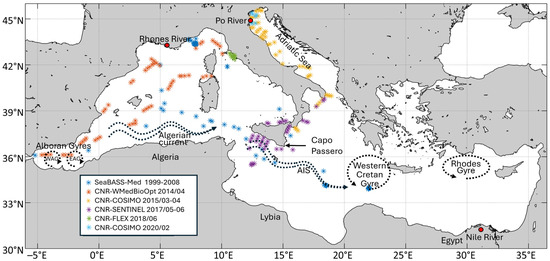
Figure 1.
Study area (Mediterranean Sea) with the spatial and temporal distribution of the in situ HPLC pigment dataset used in this work. As explained in the legend, blue dots indicate the Mediterranean subset from SeaBASS while the other colours show the CNR/ENEA in situ dataset (see Section 2.1 and Appendix A for dataset’s details).
Considering this evidence, Navarro et al. [8] and Sammartino et al. [9] investigated existing global algorithms [10,11] to assess their suitability for detecting the composition of phytoplankton assemblage in the Mediterranean Sea. In particular, Navarro et al. [8] also performed a Mediterranean regionalization of the PHYSAT method [10]. Both studies conducted a spatio-temporal analysis of the phytoplankton assemblage in the basin. However, their results are not directly comparable, providing complementary information: Sammartino et al. [9] analyzed the contribution of phytoplankton size classes (PSCs) to the total Chla, while Navarro et al. [8] studied the dominance of phytoplankton functional types (PFTs). Sammartino et al. [9]’s work was further developed by Di Cicco et al. [12], which highlighted that a regionalization for satellite estimates of phytoplankton groups (PGs) in the Mediterranean Sea is required considering its peculiar bio-optical properties. Accordingly, the authors developed regional algorithms for the specific detection of PSCs and PFTs in the Mediterranea Sea. Performing a quantitative comparison with global abundance-based models [11,13,14] applied to the same validation dataset, they showed that the regionalization improved the uncertainty and the spread of about one order of magnitude for all the classes considered. These regional algorithms have been implemented in the EU Copernicus Marine Service (or Copernicus Marine Environment Monitoring Service, CMEMS), https://www.copernicus.eu/en/copernicus-services/marine (accessed on 21 October 2025), and PSC and PFT variables have been delivered by the Ocean Colour Thematic Assembly Centre (OCTAC) since 2019 [15]. Within CMEMS, the OCTAC produces state-of-the-art OC products for the global ocean and the European seas based on multiple satellite missions, providing added-value information not readily available from space agencies [15]. OC data of PFTs and PSCs for the Mediterranean Sea provide estimates of Total-Chlorophyll a concentration in sea water (see next section for pigment details) associated with the following groups: micro-phytoplankton (MICRO), nano-phytoplankton (NANO) and pico-phytoplankton (PICO) for the PSCs, and Diatoms (DIATO), Dinophytes or Dinoflagellates (DINO), Cryptophytes (CRYPTO), Haptophytes (HAPTO), Green Algae and Prochlorococcus (GREEN) and Prokaryotes (PROKAR) for the PFTs (for details on PSC and PFT classification see Section 2.2).
Currently, Mediterranean PSC and PFT daily data starting from the end of 1997 are produced both in near-real time (NRT) and as reprocessed multiyear (MY) data, delivered as part of the daily consistently projected Level 3 “Plankton” datasets in the CMEMS products OCEANCOLOUR_MED_BGC_L3_NRT_009_141 [16] and OCEANCOLOUR_MED_BGC_L3_MY_009_143 [17], respectively [18].
One of the OCTAC’s priorities is to continue improving the accuracy of existing essential ocean variables (EOVs) at the basin level [15]. In this context, updated empirical algorithms for PFT and PSC estimates in the Mediterranean Sea are presented in this work, and the improvements in the PG retrieval are discussed. The paper is organized as follows. Data and methods are explained in Section 2, with an insight into the in situ quantification of PGs and the methods used for in situ fitting procedure and satellite data application. In Section 3, the results are presented and discussed with respect to the previous version of the algorithms described in Di Cicco et al. [12]. In addition, remarks on the new fully reprocessed multi-sensor time series of PFTs and PSCs from 1998 to 2024 released by OCTAC are addressed. Finally, conclusions are drawn in Section 4.
2. Materials and Methods
2.1. In Situ Dataset
Measurements of phytoplankton pigment concentrations obtained through High Performance Liquid Chromatography (HPLC) were used for in situ quantification of PFTs and PSCs in terms of Total-Chlorophyll a concentration (hereafter referred to as Chla and consisting of the sum of monovinyl-Chlorophyll a plus its allomers and epimers, divinyl- Chlorophyll a and Chlorophyllide a) following the approach applied in Di Cicco et al. [12]. The in situ dataset used in the previous version of the algorithm, consisting of a Mediterranean subset of the SeaWiFS Bio-optical Archive and Storage System (SeaBASS) [19] from 1998 to 2008, has been significantly improved in both spatial and temporal coverage with new data collected by the Institute of Marine Sciences of the National Research Council of Italy (CNR-ISMAR) in several measurement campaigns and analyzed at the Diagnostics and Metrology Laboratory of the Italian National Agency for New Technologies, Energy and Sustainable Economic Development (ENEA). For the CNR/ENEA HPLC dataset, details about data collection and analysis protocols are fully described in Appendix A, while the information on the timing of sample collection is provided in Figure 1. Data from the SeaBASS Mediterranean subset were collected during various research cruises and through periodic monitoring activities at fixed mooring stations. For further details on sampling times, we refer the reader to Di Cicco et al. [12].
The final dataset covered the period from 1999 to 2020. As in the previous work [12], quality assurance to build up a coherent combination of the data (collected by several teams and analyzed in different laboratories) was performed according to Trees et al. [20], Aiken et al. [21] and Hirata et al. [14]. After the quality check, our dataset consisted of 1997 useful measurements. Moreover, unlike the previous work where the dataset covered a depth range spanning from the surface to 50 m, this study focused only on the upper 10 m of the water column, which are more representative of the first optical depth, the layer at which the OC observations are limited [22,23]. This reduced the number of valid data to 1068. Figure 1 shows the study area and the spatial and temporal distribution of the final dataset.
2.2. Update of Chla-Pigment Ratios and Phytoplankton In Situ Quantification
As for Di Cicco et al. [12], the in situ quantification of PSCs and PFTs in terms of their contribution to the total Chla concentration of the assemblage was obtained through the analysis of the cell’s pigmentary content of the in situ samples, exploiting the marker properties of some pigments defined as diagnostic (DPs). Over long-time scales, climate change and/or other impacts from human activities can alter environmental conditions with potential modifications in phytoplankton assemblage structure and its pigment composition. This, in turn, can affect the Chla/DP ratios [24] required for PFT and PSC quantification, which support the algorithm calibration. To ensure more accurate estimates, the empirical relations used to compute the PFTs and PFCs through this Diagnostic Pigment Analysis (DPA) need to be re-evaluated over time [12]. Accordingly, in this work the new algorithms are calibrated with PSC and PFT in situ data derived from a new DPA based on a Mediterranean HPLC in situ dataset which has been extensively enhanced in both spatial and temporal coverage (refer to Section 2.1 and Figure 1). The regionalization of the DPA is based on earlier works carried out for global oceans [25,26,27]. Seven pigments were selected as diagnostic [28,29] for several principal groups representative of whole assemblage (see Table 1). A multiple regression analysis between the in situ total Chla and these DPs was performed, providing the best estimates of the Chla/DP ratios specific for the Mediterranean basin ().

Table 1.
Update of the best estimates (new coefficients) of Chla to DP ratios for the Mediterranean Sea with their standard deviations and significance values (p-value).
The in situ quantification of each PG, including both PFTs and PSCs, was performed by applying the newly derived DPA ratios to the same estimation formulas provided by DiCicco et al. [12]. For comprehensive methodological details, the reader is referred to that study. As in this previous work, the Sieburth et al. [30] dimensional classification was adopted for defining size classes, while for their quantification Vidussi et al. [29]’s approach with the adjustment of Brewin et al. [13] was applied, both based on the relationship between mean taxonomic types (estimated via DPs) and their most common dimensions in the Mediterranean Sea. Major taxonomic groups can also be classified into distinct functional groups according to their biogeochemical metabolic pathways or the specific resources they use and share. Thus, nitrogen fixers include Prokaryotes (ability solely of this group), calcifiers include the Haptophytes, silicifers consist of Diatoms (followed by some Chrysophytes, Silicoflagellates and Xanthophytes, which are not very widespread in the Mediterranean Sea) and Dimethylsulfoniopropionate (DMSP) producers involve primarily phytoplankton organisms belonging to the group of Dinoflagellates, followed by Haptophytes [1,12,31,32,33].
2.3. Algorithm Update
The PFT and PSC fractions of Chla concentration resulting from the in situ DPA and regression analysis were randomly divided in two independent subsets: 70% and 30% of all data, respectively, for the algorithm calibration and validation. To identify the empirical functions for each group, the in situ fractions were regressed against the corresponding log10-transformed in situ total Chla concentrations (considering the log-normal distribution of this pigment), taking into account the known co-variability existing between them [14,34]. The ordinary least square fits were used to define the functional forms that best represent the Mediterranean data distribution. The fitting procedure was performed using the curve fitting function of Matlab [35] with Bisquare robustness and Trust-region algorithm as fit options.
2.4. Satellite Dataset—Chla Data for Algorithm Application
Satellite data of PFTs and PSCs for the Mediterranean Sea for a time series from 1997 to the present at 1 km of spatial resolution are estimated by applying the updated algorithms to the respective OC multi sensor Level 3 Chla data, available on the CMEMS catalogue (product OCEANCOLOUR_MED_BGC_L3_MY_009_143 [17]). These data were produced by the CMEMS—OCTAC applying an ad hoc processing chain on Single-sensor Level 2 Remote Sensing Reflectances (Rrs) downloaded from space agencies. Observations from SeaWiFS, MERIS, MODIS-Aqua, VIIRS-NPP, VIIRS-NOAA20 and OLCI- Sentinel3A and 3B were merged into a single multi-sensor data adjusted for inter-sensor biases by applying a series of processing steps based on state-of-the-art algorithms. The Rrs spectrum obtained at this stage is used as input to compute surface Chla (nominal resolution of 1Km) via regional Ocean Colour algorithm, which will be described further on in this section. All the steps involved in the Mediterranean OC Level 3 operational multi-sensor processing are detailed in Volpe et al. [36] and Colella et al. [18]. As for the analysis performed in Di Cicco et al. [12], the specific satellite Chla used as input to produce PSC and PFT data is a blended Case 1–Case 2 field that considers the different optical properties of the offshore and inshore waters employing two distinct regional algorithms, the MedOC4.2020 [18,36] for Case 1 waters and the AD4 [37] for Case 2 waters. The exact identification of the two water types is performed by considering the whole light spectrum from blue to NIR bands for both water types from in situ data [38,39]. To categorize a satellite pixel as Case 1, Case 2, or mixed, the Mahalanobis distance between the satellite spectrum and the in situ reference spectra is computed and applied as a weight to derive the pixel’s final Chla value. The method applied, described in Colella et al. [18], also takes into account waters with high Chla concentrations resulting from phytoplankton blooms (e.g., Gulf of Lions) or mixing (e.g., Alborán Sea), which may otherwise be misclassified as Case 2 waters.
2.5. Metrics
Statistical figures used in this work for the quantitative evaluation of algorithm development are the Pearson correlation coefficient (r), Mean Bias Error (MBE), Root Mean Squared Error (RMSE), mean Relative Percentage Difference (RPD) and the mean Absolute Percentage Difference (APD), computed using the following expressions:
with XE indicating the “Estimated” dataset (satellite-based) and XM the reference dataset (in situ ”Measured”).
For the evaluation of satellite application of the algorithm, a type 2 regression is also performed, considering the dual uncertainty associated with both the in situ measurements and satellite estimates. Thus, consistently with Copernicus Marine Service metrics, two additional figures are used for satellite validation, type-2 slope (S) and type-2 intercept (I), computed with the following formulas:
To compare the results with the previous work, all the statistics are computed on linear values of PFT/PSC concentrations; thus, MBE, RMSE, S and I are expressed in mg m−3, while r, RPD and APD are dimensionless, with RPD and APD in %.
3. Results and Discussions
3.1. Regional DPA Update
The multiple regression analysis between the in situ total Chla and DPs produced highly significant results, with a determination coefficient (R2) of 0.99 between in situ and estimated Chla, and a p-value < 0.001 (based on the t-test). Table 1 summarizes all the selected DPs, their principal taxonomic meaning, and the corresponding regression coefficients with their standard deviation and statistical significance (p-value).
Although in our in situ pigment dataset the western Mediterranean Sea is more represented than the eastern Mediterranean, it includes a significant part of samples (43% of the total) that fall in the oligotrophic Chla range typical of the eastern basin (0.02–0.14 mg m−3) [12]; therefore, our dataset can be considered well-representative of all trophic regimes of the entire Mediterranean Sea. This is also proven by Gittings et al. [40], that in their work tested the results of our new DPA against their analysis based on a pigment dataset which includes a larger number of observations in the eastern Mediterranean Sea (unpublished data). Their results show good agreement between the two multiple regressions. In their work, they used an independent validation dataset of 2234 points, representative of the entire Mediterranean Sea and spanning from surface to 20 m depth. Chla obtained by the sum of weighted diagnostic pigment ratios resulting from the two different regression analyses was plotted against the in situ measured total Chla concentration The differences in the statistics are not significative, also considering that, unlike Gittings et al. [40], our DPA was developed considering only pigments from the first 10 m of the water column. The metrics show r = 0.994 vs. 0.996, Mean Absolute Error, MAE = 0.031 vs. 0.026 and MBE = −0.018 vs. 0.013, for this and their work, respectively.
Finally, applying the new DPA coefficients to the same estimation formulas provided by DiCicco et al. [12], PSC and PFT fractions of total Chla were quantified for the Mediterranean dataset.
3.2. Algorithm Update and In Situ Cal/Val
The least square fit applied to the in situ PFT and PSC fractions against the log10 of total Chla highlighted exponential functions for MICRO and DIATO, while PICO and PROKAR are well-outlined by simple cubic polynomial functions. The GREEN group continues to be well represented by a functional form proposed at global level by Hirata et al. [14], while the best result for CRYPTO is represented by a second-degree Gaussian function. Finally, NANO, DINO and HAPTO are derived as differences to comply with the mass balance. The new PSC and PFT functional forms with their coefficients are summarized in Table 2, and the algorithms are shown in Figure 2 with their calibration fit. The range of applicability is defined between 0.02 and 5.50 mg m−3 of Chla concentration.
Table 2.
New coefficients and functional forms of the updated algorithms developed for the PFT/PSC estimates in the Mediterranean Sea, where x is the log10 of Chla in mg m−3.
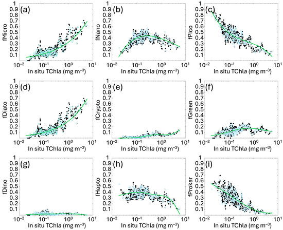
Figure 2.
New regional relationships obtained fitting the fractions f of each size class (MICRO, NANO and PICO, panels (a–c)) and functional type (DIATO, CRYPTO, GREEN, DINO, HAPTO and PROKAR, panels (d–i)) estimated with the diagnostic pigments, against the in situ total Chla concentration (as detailed in Section 2.2). Black and light blue dots represent calibration and validation data, respectively. The green line indicates the best fitting curve for the calibration dataset for each group. The functions are described in Table 2.
The increased spatial and temporal coverage of the in situ dataset has resulted, in some cases, in changing the mathematical functions that best fit the distribution of data-points, particularly for MICRO, DIATO and CRYPTO, previously represented by simple cubic polynomial functions. Also, in the former version, PICO was derived as difference instead of NANO. These changes reflect the variations in the pigment ratios between Chla and DPs, resulting from the improved spatial and temporal resolution of the dataset, as well as the reduced investigating depth.
The algorithm hindcast evaluation (i.e., a first algorithm evaluation using the same in situ fitting calibration subset also for testing) and the in situ validation with the independent subset are presented in Figure 3, with a detailed summary of their statistical assessment provided in Table 3. Both metrics and scatter plots show the goodness of the fits for all the groups considered, with statistical values of validation consistent with calibration/hindcast evaluation. The Pearson correlation coefficient (Table 3) shows high correlation with values ranging from 0.78 to 0.99 and improves with respect to Di Cicco et al. [12], particularly for PICO (previous r = 0.88 vs. 0.93 in this work) and DINO (previous r = 0.60 vs. 0.87 in this work). For the other groups, values span between 0.94 and 0.99. Regarding bias, although MBE has slightly increased for some groups, variations are limited to the order of 10−3 mg m−3; thus, it remains essentially constant. Regarding the spread of the estimated values around the in situ measured data (error distribution), RMSE improved for most groups, previously ranging from 0.018 to 0.070 mg m−3 and now decreased within a range of 0.006–0.059 mg m−3.
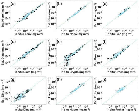
Figure 3.
In situ hindcast evaluation and independent validation of the new algorithms obtained comparing the Chla concentration of each size class (panels (a–c)) and functional type (panels (d–i)) derived from the diagnostic pigments (as detailed in Section 2.2) with the same quantity estimated by applying the new functions to the in situ total Chla. Black and light blue dots represent calibration and validation data, respectively. The green dotted line represents the 1:1 line. For the metrics, refer to Table 3.
Table 3.
Statistical results of the updated algorithms applied to the in situ calibration (hindcast evaluation) and validation subsets (respectively, 70% and 30% of the entire dataset). The statistics are computed on linear Chla concentration values (mg m−3). MBE and RMSE are expressed in mg m−3, while r, RPD and APD are dimensionless.
Overall, the validation results show either improvements or consistency across all metrics, compared to previous algorithms, for both PFT and PSC groups. These results are also confirmed by the mean Relative and Absolute Percentage Differences (RPD and APD), which also consider the different dynamical range of Chla concentration of each class. Weighing the uncertainty on the dynamical range of the observed concentration values, statistical data confirmed the goodness of the fits.
3.3. Satellite PFT and PSC Estimates—Validation Matchup Analysis
The results of validation analysis of satellite PFT and PSC estimates for the Mediterranean Sea are shown in Figure 4. L3 daily multi-sensor PG data retrieved by applying the new algorithms to the satellite Chla were compared with the corresponding PG-Chla in situ concentrations. For all groups (Figure 4), the values of the PFT and PSC data span over two or three orders of magnitude, except for PICO and even more for PROKAR groups, whose Chla concentrations are distributed in a very narrow range (between about 0.01 and 0.2 mg m−3).
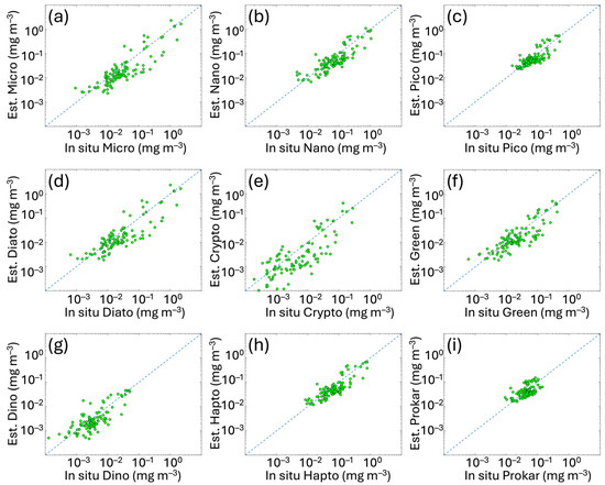
Figure 4.
Regional satellite estimates (y axes) vs. in situ PSC and PFT Chla concentrations for the Mediterranean Sea. The panels represent the matchup validation for the following groups: (a) MICRO, (b) NANO and (c) PICO (for the PSCs), and (d) DIATO, (e) CRYPTO, (f) GREEN, (g) DINO, (h) HAPTO and (i) PROKAR (for the PFTs). Green dots represent the validation data. The 1:1 line is shown as blue dotted line. For the metrics, refer to Table 4.
In Table 4, the metrics of the validation analysis are provided and compared to the statistical values of the previous algorithm validation obtained by applying the same CMEMS Chla data. Results highlight that PFT and PSC estimates based on the updated version of the algorithms show improvements for most groups. MBE and r improve for all groups, with r remaining unchanged only for PROKAR and HAPTO. The MBE, ranging from −0.001 to −0.023 mg m−3, decreases significantly in some cases (e.g., for MICRO, NANO and DIATO, changing from −0.044 to −0.022 mg m−3, −0.045 to −0.023 mg m−3 and 0.041 to −0.021 mg m−3, respectively), reducing the underestimation that affected the previous retrieval. However, the small negative bias also visible throughout the entire dynamic range for all the groups (Figure 4) seems to follow the bias of input chlorophyll itself. This also occurred in the previous version of the PFT/PSC algorithm, although here is reduced (see Figure A1 in Appendix B). This is evident by performing a matchup analysis for the sole satellite Chla using the co-located in situ Chla corresponding to the PFT/PSC validation datapoints and coming from the same dataset (Section 2.1 and Figure 1). In Figure A1, scatterplots and statistics of this Chla analysis are shown, respectively, for the 2023 (on the left) and 2024 (on the right) CMEMS Entry Into Service (EIS), with the former still including the PFT/PSC algorithm of Di Cicco et al. [12] and the latter the updated version presented here. The same algorithm is used for the input Chla satellite estimates, both for 2023 and 2024 EIS.
Table 4.
Statistical results from the satellite validation of the updated algorithms compared with the previous functions using the same validation dataset, consisting of thesatellite data available in the validation subsets (match-up analysis). The statistics are computed on linear Chla concentration values (mg m−3). MBE, RMSE, S and I are expressed in mg m−3, while r, RPD and APD are dimensionless.
Regarding the spread of the estimated values around the in situ observed ones, this narrows, especially for NANO, DINO and CRYPTO, which are also joined by DIATO, DINO and GREEN when considering the different dynamic range of Chla concentration represented by each class, as shown by the APD values in Table 4. Good results were also achieved by the type-2 slopes, which are much closer to one for most groups, indicating that the new models compare better with the in situ data than the previous ones.
Although, as expected, the good agreement between the regional models and the in situ data observed in the in situ validation (Table 3) partially deteriorated when the models were applied to satellite Chla (Table 4), nevertheless the metrics show good consistency with the in situ validation analysis, and the results highlight improved performances and better predictive power with respect to the previous models. Using an independent dataset representative of the entire Mediterranean Sea consisting of 2234 points (details are provided in Section 3.1), Gittings et al. [40] also compared our PSC algorithms (PICO, NANO, and MICRO) with the corresponding models of Brewin et al. [13] re-parameterized for the Mediterranean Sea in their work. The results demonstrated that both approaches are valid for deriving satellite-based observations of phytoplankton size structure in the Mediterranean Sea.
3.4. Phytoplankton Variability in the Mediterranean Sea: Satellite PFT and PSC Analysis
Once the suitability of the new functions for the Mediterranean Sea was demonstrated, the new algorithms were implemented in CMEMS and applied to a time series of about 27 years of Chla data, producing a new fully reprocessed multi-sensor time series of PFTs and PSCs from 1998 to 2024. Figure 5 (top panels) shows the monthly climatology with its standard deviation of each PG over the whole Mediterranean Sea, both in terms of size and type obtained applying the updated algorithms. The results are compared with the same analysis performed applying the previous models to the same satellite Chla time series (Figure 5, bottom panels). In general, the behaviour of the various groups is quite consistent with the previous algorithm. Nevertheless, significant changes are evident. As in the previous version, the monthly climatology analysis shows that, at basin scale, the dominant size groups are NANO and PICO, with the former prevailing in winter–early spring and the latter from May through the entire autumn. These agree with the results also observed in El Hourany et al. [41], who studied phytoplankton diversity in the Mediterranean Sea using the GlobColour satellite dataset (https://data.marine.copernicus.eu/ (accessed on 21 October 2025)) and applying a Self-Organizing Map (SOM) approach. In terms of functional types, the primary PGs contributing to total Chla are Haptophytes, which remain the dominant group throughout the year, followed by Diatoms and Prokaryotes, which alternate in prevalence, and then by Green Algae. Compared to previous models, a notable increase in the contribution of the Green Algae to Chla is observed throughout the year, in contrast to the DINO and CRYPTO groups, which show a decreasing trend. These observations align with the results of El Hourany et al. [41], in which CRYPTO is largely absent across most of the basin, while Chlorophytes are more broadly distributed across the year and throughout the entire basin. DINO remains the group with the lowest overall concentrations. The contribution of Diatoms to Chla is greater than that of Prokaryotes for a longer period, from October until May, when the total Chla concentration starts to decrease and the trend reverses, with Prokaryotes surpassing Diatoms, a condition that persists until September.
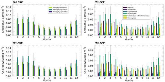
Figure 5.
Mean monthly climatology (1998–2024) of PSC (A,C) and PFT (B,D) contribution to the total Chla (mg m−3) over the whole Mediterranean Sea. The results obtained applying the new updated algorithms (A,B) are compared with the same analysis performed, applying the previous algorithms [12] to the same satellite Chla time series (C,D).
Another significant difference is observed in the PICO-size class, showing a greater contribution to total Chla throughout the year than in the previous algorithm. As a result, during the fall–winter period, its concentrations are closer to those of NANO, and in the months when dominance reverses, the gap between them increases in favour of PICO. MICRO, on the other hand, remains constant on average. The results obtained in the PSC’s monthly climatology analysis show a shift in favour of smaller cells in the contribution to Chla, which are consistent with the general trend observed in the phytoplankton assemblage structure in the Mediterranean Sea at both basin and sub-basin scales [40,42,43,44]. As additional insight, the standard deviation highlights greater variability in the Chla concentration associated with larger size classes (MICRO and NANO for the PSCs, and DIATO and HAPTO for the corresponding PFTs) during the winter–early spring months. This reflects the marked intensification of the trophic gradient that typically distinguishes the western Mediterranean from the eastern basin at this time of year.
To provide a summary view of phytoplankton temporal and spatial variability in the Mediterranean Sea, PSC-Chla monthly concentrations were analyzed from 1998 to 2024 along a series of transects encompassing the most representative trophic areas in the basin, as previously performed by Navarro et al. [8] following the approach of D’Ortenzio and Ribera d’Alcalà [22]. In particular, the analysis was conducted along four transects shown in Figure 6 and Figure 7, superimposed on monthly maps representing different seasonal conditions (March and July for spring and summer, respectively, for the year 2022): a west-to-east zonal transect, extending from the Alborán Sea to the east coast of the Aegean Sea; two meridional transects, the first in the western Mediterranean Sea (WMMT), extending from the Gulf of Lion to the Algerian coasts, and the second in the eastern Mediterranean Sea (EMMT), originating east of Rhodes and extending to the Egyptian coast; and a final combined transect, running across the entire Adriatic Sea and proceeding meridionally through the full extent of the central Mediterranean basin (CMMT). The results are presented through Hovmöller diagrams [45] and show the variability of the monthly time series of PSCs along longitude for the zonal transect (Figure 6) and along latitude for the meridional and combined transects (Figure 7). The diagrams allow observation of how the contributions of the three size classes to the total Chla vary spatially and temporally in response to changes in Chla itself.
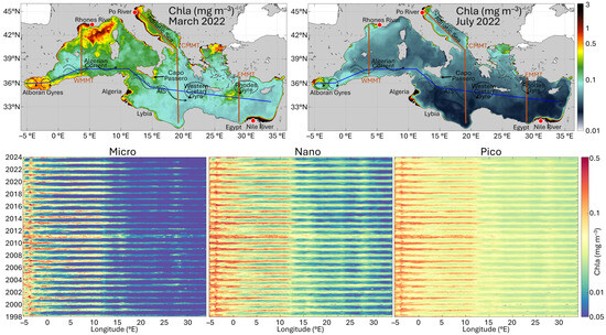
Figure 6.
Analysis of the monthly climatology time series of the three PSCs in the Mediterranean Sea along a west–east transect. Top panel: Monthly Chla maps of the Mediterranean Sea representing two opposite phases of the seasonal cycle, i.e., March 2022 for spring (on the left) and July 2022 for summer (on the right). Superimposed onto the maps, the zonal west–east transect (blue line), and the three Meridional Transects (red line): Western (WMMT), Central (CMMT) and Eastern Mediterranean (EMMT). Bottom panel: Hovmöller diagrams showing the variability of the monthly time series of PSCs (MICRO, NANO and PICO from left to right, respectively) along longitude for the zonal transect.
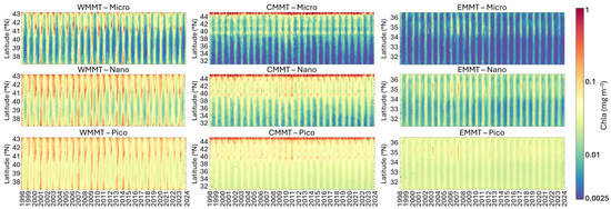
Figure 7.
Analysis of the monthly climatology time series of the three PSCs in the Mediterranean Sea along two meridional transects, the former in the West Mediterranean Sea (WMMT, to the left) and the latter in the East Mediterranean Sea (EMMT, to the right), and a combined transect running across the entire Adriatic Sea and proceeding meridionally through the full extent of the central Mediterranean basin (CMMT, to the centre). The Hovmöller diagrams show the variability of the monthly time series of MICRO, NANO and PICO (from top to bottom, respectively) for each transect.
Observing the Howmöller diagrams in the W-E transect (Figure 6), the basin results divided into two distinct zones (approximately at 12°E), reflecting the west to east gradients in phosphate and nitrate concentrations [7,46]:
- (1)
- The first zone is located in the western basin, between about −5°E and 12°E. In this area, Chla concentrations reach maximum values in all three groups, with a general dominance of NANO, especially between October and April. Overall, the contribution of PICO is also significant in these areas, becoming dominant between −3°E and 12°E in the more oligotrophic months of the year, between May and September, where MICRO is almost absent and NANO becomes the second most important size group. In the Alborán basin, where the Western Alborán Gyres (WAG) exhibits a clear seasonal cycle with the intensification beginning in summer [47], the dominance of MICRO is observed during the winter–spring months, when the spatio-temporal variability of Chla concentration driven by the anticyclonic WAG seems to be particularly pronounced. Crossing the gyre between −5°E and −3°E, higher Chla concentrations are observed for all groups along the gyre edge, while lower concentrations are clear in the centre. On the edge, concentrations remain relatively elevated throughout most of the year, whereas in the centre of the gyre a more pronounced seasonal variability is observed. This is also evident in the Chla map of July in Figure 6. In particular, the gyre’s interior is dominated by PICO and NANO, with very low Chla values of MICRO, while in the gyre edge Chla is characterized by the dominance of MICRO followed by NANO, although all three groups exhibit higher contributions. As a general behaviour, a decrease in the concentration of all groups is observed over time, likely due to a general decrease in Chla concentrations, well-evident particularly inside the gyre. This appears consistent with Abdellaoui et al. [48], who analyzed Sea Surface Temperature (SST) and Chla trends based on 20 years (2001–2020) of satellite data in relation to hydrodynamic processes in the Alborán Sea. They found in the same area a Chla decline probably due to sea surface warming affecting the vertical mixing and the metabolic responses of phytoplankton assemblage.
- (2)
- In the Central-Eastern Mediterranean basin (from approximately 12°E eastward), total Chla mostly consists of PICO and NANO groups, with PICO dominating mainly in the Eastern zone and particularly in the months between May and November, when an important decrease in NANO contributions is evident. Areas with NANO and PICO Chla concentration exceeding the eastern basin-wide average are consistently observed throughout the entire time series, exhibiting a less-pronounced seasonal cycle with peak values during winter and early spring.
Specifically, three regions are identified: (i) between 15°E and 16°E, off “Capo Passero” (southeast of Sicily), where the Atlantic Ionian Stream (AIS) intensifies during winter, advecting high-chlorophyll coastal waters offshore in a filament-like structure [49]; (ii) between 23°E and 24°E, possibly associated with the Western Cretan Gyre; and (iii) between 27°E and 28°E, corresponding to the cyclonic Rhodes Gyre. Notably, the highest Chla values for all three groups in this region were detectable during the spring of 2022 (Figure 6, monthly maps), accordingly with Teruzzi et al. [50]. They highlighted an unusual phytoplankton bloom in a large area southeast of Crete in 2022, more intense than typical of about 50% (Figure 6, both monthly maps and Hovmöller diagrams), caused by a winter anomalous sea surface cooling event which impacted deep convection and thus nutrient input to the euphotic layer [51].
Considering the entire W-E transect, the seasonal variability in the three size groups is well-evident, with the greatest variations experienced by MICRO in the western area of the transect. Furthermore, the analysis of the entire time series shows a shift in the seasonal dynamics of phytoplankton assemblage. A distinct period is observed from late 2010 through all of 2011, during which all groups experience the longest sustained phase of elevated concentrations.
Figure 7 summarizes the analysis results for the two meridional transects (in the western and eastern Mediterranean Sea) and the combined transect (covering the Adriatic Sea and central Mediterranean Sea), all of which encompass different trophic zones [22,52]:
- (1)
- In the western transect (WMMT), extending from the Gulf of Lion to the Algerian coast (Figure 7, left panel), all three size classes exhibit a pronounced seasonal cycle, with the highest and most persistent concentrations observed in the Gulf of Lion. This area is characterized by elevated productivity, primarily driven by substantial nutrient inputs from the Rhône River, from offshore waters, and seasonal upwelling and mixing processes [53]. In particular, between 39°N and 41°N, the MICRO size class appears to dominate almost every year during March to April/May, although NANO and PICO fractions contribute significantly. During the more oligotrophic months, typically from June to October, the PICO group becomes dominant, followed by NANO. The intermediate latitudinal band shows generally lower concentrations, which increase again near the Algerian Current. Periods of elevated concentrations across the entire transect are observed in specific years, notably 2001, 2006–2010, 2013–2014, and 2018, likely linked to changes in the North Atlantic Oscillation (NAO), which appears to exert a stronger influence than ENSO on Chla variations in the western Mediterranean Sea [52].
- (2)
- In the second transect (CMMT), running across the entire Adriatic Sea and proceeding meridionally through the full extent of central Mediterranean basin (Figure 7, central panel), the composition of the assemblage in terms of size shows quite stable behaviour. In all seasons, the highest Chla values for all three groups can be observed in the northern part of the Adriatic Sea, dominated by NANO and MICRO, where nutrient input from Po River discharge primarily drives phytoplankton biomass and primary production. Extending southward to approximately 39°N, concentrations remain relatively elevated. However, the main contribution comes from NANO and PICO. In contrast to the northern region, at this latitude a clear seasonal pattern emerges, characterized by higher concentrations from late autumn to late spring, alternating with a period of lower Chla values per group during the remaining months, in which PICO becomes dominant. As the transect extends through the entire central Mediterranean, all three groups reach their lowest concentrations and the seasonal cycle becomes more defined, with the period of highest concentrations narrowing to just a few months between winter and spring.
- (3)
- The last transect (EMMT), which crosses the eastern Mediterranean Sea latitudinally (Figure 7, right panel), is characterized by the lowest concentrations of Chla for all groups, with the increase in concentrations for very short periods of the year, mainly between late winter–spring, generally dominated by PICO and NANO. The highest concentrations for all groups are observed in correspondence to the Rhodes gyre (Figure 7, top panel). Here, a cyclic increase in Chla concentrations across all three size classes is observed approximately every 4–5 years, with particularly intense events in 2003, 2006 and 2007.
Overall, in the years 2003 and 2006–2007, significant increases in total Chla are observed in both the western and eastern transects during late winter to early spring, resulting in concentration changes in all PSCs and a shift in the assemblage composition toward a dominance of larger-sized groups. Specifically, Basterretxea et al. [52] analyzed the regional influences of the North Atlantic Oscillation (NAO) and El Niño Southern Oscillation (ENSO) on long-term (>1 year) Chla variability. Their analysis revealed a significant regime shift occurring in 2004–2007, when NAO transitioned from positive to negative phase, notably affecting phytoplankton biomass and highlighting changes at the ecosystem level driven by climate in the Mediterranean Sea.
4. Conclusions
The update of the PSC and PFT algorithms within the Copernicus Marine Service has improved model performance compared to Di Cicco et al. [12], where regionalization was crucial for enhancing phytoplankton group estimates. Analysis of the new 27-year monthly climatology time series of PG satellite data demonstrated consistency and coherence with the previous series, as well as with the existing literature, for both PFTs and PSCs. However, the updated models reveal significant variations in individual group contributions to total Chla, as they are based on more accurate pigment ratios (Chla/DP ratio) representative of a broader temporal range. The climatological analysis indicates NANO and PICO as dominant size classes, with NANO prevailing during winter–early spring, while PICO surpasses it from May through the entire autumn. This pattern is mirrored in the functional composition, with Haptophytes dominating year-round, followed by Diatoms and Prokaryotes, which alternate in prevalence during the year, and then by Green Algae, whose contribution increased markedly compared to the previous model. As general behaviour, the PICO-size class contributes more to total Chla throughout the year, reducing the gap with NANO during the fall–winter period and indicating an overall shift toward smaller phytoplankton cells, consistent with general trends observed in the Mediterranean Sea. These changes reflect shifts in the assemblage structure in terms of group evenness and dominance, both taxonomic and dimensional. This suggests a potential shift in phytoplankton diversity, not only structurally but also in the processes driving assemblage organization [54].
The Chla-abundance approach has shown valid results for the retrieval of phytoplankton diversity in the Mediterranean Sea. However, in view of new-generation sensors, spectral response-based approaches should be investigated to obtain higher-resolution information on phytoplankton assemblage composition by exploiting hyperspectral data and more refined spectral signatures. A broad consensus exists within the OC research and user communities that enhancing satellite-based resolution of phytoplankton diversity will significantly advance our comprehension of marine ecosystems, ocean health, impacts of climate variability on biogeochemical cycle and mitigation roles of biological processes [55]. The prioritization of hyperspectral satellite missions by space agencies, e.g., NASA’s Plankton, Aerosol, Cloud, ocean Ecology (PACE) mission [56], is expected to substantially address the capabilities required to fill this gap. In this context, the methods used for the in situ quantification of the assemblage composition remain a key point, as they are ultimately employed for the calibration and/or validation activities of satellite models. A critical analysis of the various methods has already been conducted and well-documented in [55,57,58], and we refer to their works for a more in-depth discussion. However, we consider it crucial to emphasize that, at the current state of the art, no single method is able to capture the full diversity of marine phytoplankton, although each method provides valuable specific information that helps to describe and model phytoplankton assemblage composition [55]. Based on the main datasets currently available for both global and basin-scale studies, most current approaches for developing algorithms for satellite PG estimates rely on pigment-based methods to quantitatively calibrate and validate the models. The composition and concentrations of the accessory pigments strongly influence the variability in shape and magnitude of phytoplankton absorption [59,60,61], thereby affecting the resulting Rrs [62]. Nevertheless, phytoplankton pigments lack high taxonomic resolution and can only provide indirect information about community structure. In addition, pigment concentrations can be modulated also by cellular physiology, which is affected in turn by biotic and abiotic drivers. This can decouple pigment signals, making ambiguous the taxonomic interpretation for certain pigments [60,63,64]. We believe that, especially in light of forthcoming hyperspectral radiometric acquisitions, the scientific community should invest greater effort in collecting more comprehensive biological datasets [2,65]. The use of pigments to assess in situ phytoplankton composition should not be considered a replacement for direct methods, (e.g., microscopy-based approach, flow-cytometry and imaging flow-cytometry techniques) which provide absolute quantitative information at a higher taxonomic level, but complementary information, contributing to a comprehensive characterization of the community. New technologies must be explored and/or implemented to improve in situ knowledge and enable more user-friendly and rapid systems capable of accurately representing the entire community in terms of absolute quantification. Technological development is required, particularly toward continuous acquisition systems such as imaging flow-cytometry, which allow automated single-cell discrimination at species-level resolution and generate image datasets suitable for AI-based classification [66,67]. However, these methods still remain limited by size range, typically covering only 6–150 µm, thus spanning only part of the nano- and micro-phytoplankton. In this context, molecular approaches, especially DNA metabarcoding, offer strong potential for providing species-level resolution across the full-size spectrum. Yet, the resulting data and most available datasets are still largely compositional (i.e., relative, not absolute abundances) and often not directly comparable. Efforts are ongoing to develop quantitative DNA-based methods, such as the use of internal standards ([55,68], and references therein). Finally, we emphasize the importance of expert working groups to coherently integrate data from different approaches, each providing a unique perspective on the assemblage [65]. Indeed, achieving consistent integration across different data types (both relative and absolute) and size ranges, ensuring full coverage of the size spectrum without artificial gaps or overlaps due to methodological limitations, remains a major challenge to date [55].
Author Contributions
Conceptualization, A.D.C. and V.E.B.; methodology, A.D.C.; software, A.D.C., M.S., G.V. and S.C.; validation, A.D.C., V.E.B., F.A., G.V. and S.C.; formal analysis, A.D.C.; investigation, A.D.C.; resources, A.D.C., V.E.B., F.A. and A.L.; satellite data curation, A.D.C., M.S. and S.C.; in situ data curation, A.D.C., F.A. and I.G.; writing—original draft preparation, A.D.C.; writing—review and editing, A.D.C., M.S., V.E.B., F.A., A.L., I.G., G.V., G.M.P., C.L. and S.C.; visualization, A.D.C., M.S. and G.V.; project administration, V.E.B. and C.L.; funding acquisition, V.E.B. All authors have read and agreed to the published version of the manuscript.
Funding
This work has been performed in the context of the Ocean Colour Thematic Assembly Centre (OC-TAC) of the Copernicus Marine Service (grant number: 21001L2-COP-TAC OC-2200 and 24251L03-COP-TAC OC-2200).
Data Availability Statement
The multi-sensor Level-3 Chla and PFT/PSC time series are available for download on the CMEMS web portal (https://marine.copernicus.eu/ accessed on 21 October 2025) as part of the dataset PLANKTON in the product OCEANCOLOUR_MED_BGC_L3_MY_009_143.
Acknowledgments
The authors acknowledge the SeaBASS archive for the in situ bio-optical dataset, available for free at https://seabass.gsfc.nasa.gov/ (accessed on 21 October 2025). We would like to thank Vega Forneris and Flavio Lapadula for maintaining the satellite data processing and data archive at CNR-ISMAR. We are also grateful to Marco Talone (ICM-CSIC) and Francesco Bignami (CNR-ISMAR) for their very helpful scientific advice. We sincerely thank all the researchers and technical staff involved in the CNR cruises, in both the organization and sampling activities, and all the captains and crews on board the research vessels for their valuable contributions to this study. We thank the four anonymous reviewers and the editor for their constructive comments that helped strengthening the manuscript.
Conflicts of Interest
The authors declare that the research was conducted in the absence of any commercial or financial relationships that could be construed as a potential conflict of interest.
Abbreviations
The following abbreviations are used in this manuscript:
| PSCs | Phytoplankton Size Classes |
| PFTs | Phytoplankton Functional Types |
| CMEMS | Copernicus Marine Environment Monitoring Service |
| PGs | Phytoplankton Groups |
| OCTAC | Ocean Colour Thematic Assembly Centre |
| OC | Ocean Colour |
| MICRO | Micro-phytoplankton |
| NANO | Nano-phytoplankton |
| PICO | Pico-phytoplankton |
| DIATO | Diatoms |
| DINO | Dinophytes or Dinoflagellates |
| CRYPTO | Cryptophytes |
| HAPTO | Haptophytes |
| GREEN | Green Algae and Prochlorococcus |
| PROKAR | Prokaryotes |
| EOVs | Essential Ocean Variables |
| HPLC | High Performance Liquid Chromatography |
| Chla | Total-Chlorophyll a, sum of: monovinyl-Chlorophyll a plus its allomers and epimers, divinyl-Chlorophyll a and Chlorophyllide a |
| DPA | Diagnostic Pigment Analysis |
| DPs | Diagnostic Pigments |
| Rrs | Remote Sensing Reflectances |
| r | Pearson Correlation Coefficient |
| MBE | Mean Bias Error |
| RMSE | Root Mean Squared Error |
| RPD | Mean Relative Percentage Difference |
| APD | Mean Absolute Percentage Difference |
| S | Type-2 slope |
| I | Type-2 intercept |
| R2 | Determination coefficient |
| MAE | Mean Absolute Error |
| EIS | Entry Into Service |
| SOM | Self-Organizing Map |
| WAG | Western Alborán Gyre |
| NAO | North Atlantic Oscillation |
| ENSO | El Niño Southern Oscillation |
Appendix A
In Situ Data Collection and Analysis Protocols for the CNR/ENEA Phytoplankton Pigment Dataset
Sample Collection and Storage: Sea water for sample preparation was collected in the upper 10 m of the water column using either Niskin bottles mounted on a Rousette carousel or horizontal Van Dorn bottles. During sampling, water was prefiltered with 250 µm mesh net to avoid the presence of zooplankton organisms. Known volumes of sampled water were then gently filtered through Whatman GF/F glass-fibre filters (25 mm diameter, nominal pore size of 0.7 µm) under mild vacuum not exceeding 150 mm Hg in order to minimize potential cell damage [69,70]. Finally, the filters were immediately flash frozen in liquid nitrogen and subsequently stored either in nitrogen or at −80 °C until analysis in the laboratory.
Pigment Extraction and HPLC Analysis: HPLC pigment analyses were performed using a modified version of Wright et al. [71]’s method. The method was validated by participating in international intercomparison exercises [72]. After the addition of 2 mL of 100% acetone, filters were soaked at 4 °C for 24 h to facilitate pigment extraction and finally sonicated in an ice-cold bath for 10 min. The supernatant was clarified by centrifugation at 400 rpm for 20 min at 4 °C. Prior to HPLC injection, all extracts were further filtered with a 0.2 µm porosity syringe filter and combined with water (2:1 ratio) in order to prevent peak distortion of early eluting pigments. Chromatographic analysis was performed using an Agilent Technologies 1260 HPLC system equipped with a temperature-controlled autosampler, a quaternary pump and a diode array detector. Pigments were separated on a Supelco Ascentis (Darmstadt, Germany) C18 column (25 cm, 4.6 mm internal diameter, 5 µm particle size) using a linear ternary gradient at a flow rate of 1 mL/min with three phases (Methanol: 0.5 M ammonium acetate, 80:20 v/v (phase A), Acetonitrile: water 90:10 v/v (phase B), and Ethyl Acetate (phase C)). Pigments were detected at multiple wavelengths: 450 nm for most chlorophylls and carotenoids, 436 nm for Chlorophyllide a and 667 nm for phaeopigments. The identification and quantification were performed using certified pigment standards (DHI Lab Products, Hørsholm, Denmark).
Appendix B
Comparison of Satellite Chla Validation Based on Chla-PSC/PFT Validation Datasets

Figure A1.
Scatterplots and metrics of satellite daily multi-sensor L3 Chla estimates (y-axis) and the co-located in situ Chla, corresponding to the two in situ datasets used for the PSC/PFT validation, respectively, for the 2023 (on the left) and 2024 (on the right) CMEMS Entry Into Service (EIS). The same algorithm is used for the satellite estimates both for 2023 and 2024 EIS.

References
- IOCCG. Phytoplankton Functional Types from Space; Sathyendranath, S., Ed.; Reports of the International Ocean Colour Coordinating Group; IOCCG: Dartmouth, NS, Canada, 2014; Volume 15. [Google Scholar]
- Bracher, A.; Bouman, H.A.; Brewin, R.J.W.; Bricaud, A.; Brotas, V.; Ciotti, A.M.; Clementson, L.; Devred, E.; Di Cicco, A.; Dutkiewicz, S.; et al. Obtaining Phytoplankton Diversity from Ocean Color: A Scientific Roadmap for Future Development. Front. Mar. Sci. 2017, 4, 55. [Google Scholar] [CrossRef]
- Mouw, C.B.; Hardman-Mountford, N.J.; Alvain, S.; Bracher, A.; Brewin, R.J.W.; Bricaud, A.; Ciotti, A.M.; Devred, E.; Fujiwara, A.; Hirata, T.; et al. A Consumer’s Guide to Satellite Remote Sensing of Multiple Phytoplankton Groups in the Global Ocean. Front. Mar. Sci. 2017, 4, 41. [Google Scholar] [CrossRef]
- Volpe, G.; Santoleri, R.; Vellucci, V.; Ribera d’Alcalà, M.; Marullo, S.; D’Ortenzio, F. The Colour of the Mediterranean Sea: Global versus Regional Bio-Optical Algorithms Evaluation and Implication for Satellite Chlorophyll Estimates. Remote Sens. Environ. 2007, 107, 625–638. [Google Scholar] [CrossRef]
- Lacombe, H.; Gascard, J.C.; Gonella, J.; Bethoux, J.P. Response of the Mediterranean to the Water and Energy Fluxes across Its Surface, on Seasonal and Interannual Scales. Oceanol. Acta 1981, 4, 247–255. [Google Scholar]
- Robinson, A.R.; Golnaraghi, M. The Physical and Dynamical Oceanography of the Mediterranean Sea. In Ocean Processes in Climate Dynamics: Global and Mediterranean Examples; Springer: Dordrecht, The Netherlands, 1994; pp. 255–306. [Google Scholar]
- Siokou-Frangou, I.; Christaki, U.; Mazzocchi, M.G.; Montresor, M.; Ribera d’Alcalá, M.; Vaqué, D.; Zingone, A. Plankton in the Open Mediterranean Sea: A Review. Biogeosciences 2010, 7, 1543–1586. [Google Scholar] [CrossRef]
- Navarro, G.; Alvain, S.; Vantrepotte, V.; Huertas, I.E. Identification of Dominant Phytoplankton Functional Types in the Mediterranean Sea Based on a Regionalized Remote Sensing Approach. Remote Sens. Environ. 2014, 152, 557–575. [Google Scholar] [CrossRef]
- Sammartino, M.; Di Cicco, A.; Marullo, S.; Santoleri, R. Spatio-Temporal Variability of Micro-, Nano- and Pico-Phytoplankton in the Mediterranean Sea from Satellite Ocean Colour Data of SeaWiFS. Ocean Sci. 2015, 11, 759–778. [Google Scholar] [CrossRef]
- Alvain, S.; Moulin, C.; Dandonneau, Y.; Bréon, F.M. Remote Sensing of Phytoplankton Groups in Case 1 Waters from Global SeaWiFS Imagery. Deep Sea Res. Part Oceanogr. Res. Pap. 2005, 52, 1989–2004. [Google Scholar] [CrossRef]
- Brewin, R.J.W.; Devred, E.; Sathyendranath, S.; Lavender, S.J.; Hardman-Mountford, N.J. Model of Phytoplankton Absorption Based on Three Size Classes. Appl. Opt. 2011, 50, 4535. [Google Scholar] [CrossRef]
- Di Cicco, A.; Sammartino, M.; Marullo, S.; Santoleri, R. Regional Empirical Algorithms for an Improved Identification of Phytoplankton Functional Types and Size Classes in the Mediterranean Sea Using Satellite Data. Front. Mar. Sci. 2017, 4, 126. [Google Scholar] [CrossRef]
- Brewin, R.J.W.; Sathyendranath, S.; Hirata, T.; Lavender, S.J.; Barciela, R.M.; Hardman-Mountford, N.J. A Three-Component Model of Phytoplankton Size Class for the Atlantic Ocean. Ecol. Model. 2010, 221, 1472–1483. [Google Scholar] [CrossRef]
- Hirata, T.; Hardman-Mountford, N.J.; Brewin, R.J.W.; Aiken, J.; Barlow, R.; Suzuki, K.; Isada, T.; Howell, E.; Hashioka, T.; Noguchi-Aita, M.; et al. Synoptic Relationships between Surface Chlorophyll- a and Diagnostic Pigments Specific to Phytoplankton Functional Types. Biogeosciences 2011, 8, 311–327. [Google Scholar] [CrossRef]
- Brando, V.; Santoleri, R.; Colella, S.; Volpe, G.; Di Cicco, A.; Sammartino, M.; González Vilas, L.; Lapucci, C.; Böhm, E.; Zoffoli, M.; et al. Overview of Operational Global and Regional Ocean Colour Essential Ocean Variables Within the Copernicus Marine Service. Remote Sens. 2024, 16, 4588. [Google Scholar] [CrossRef]
- European Union-Copernicus Marine Service. Mediterranean Sea, Bio-Geo-Chemical, L3, Daily Satellite Observations (Near Real Time). 2022. Available online: https://data.marine.copernicus.eu/product/OCEANCOLOUR_MED_BGC_L3_NRT_009_141/description (accessed on 21 October 2025).
- European Union-Copernicus Marine Service. Mediterranean Sea, Bio-Geo-Chemical, L3, Daily Satellite Observations (1997-Ongoing). 2022. Available online: https://data.marine.copernicus.eu/product/OCEANCOLOUR_MED_BGC_L3_MY_009_143/description (accessed on 21 October 2025).
- Colella, S.; Brando, V.E.; Di Cicco, A.; D’Alimonte, D.; Forneris, V.; Bracaglia, M. Quality Information Document for Ocean Colour Mediterranean and Black Sea Observation Product Release 4.0; Mercator Ocean International: Toulouse, France, 2024. [Google Scholar]
- Werdell, P.J.; Bailey, S.W. An Improved In-Situ Bio-Optical Data Set for Ocean Color Algorithm Development and Satellite Data Product Validation. Remote Sens. Environ. 2005, 98, 122–140. [Google Scholar] [CrossRef]
- Trees, C.C.; Clark, D.K.; Bidigare, R.R.; Ondrusek, M.E.; Mueller, J.L. Accessory Pigments versus Chlorophyll a Concentrations within the Euphotic Zone: A Ubiquitous Relationship. Limnol. Oceanogr. 2000, 45, 1130–1143. [Google Scholar] [CrossRef]
- Aiken, J.; Pradhan, Y.; Barlow, R.; Lavender, S.; Poulton, A.; Holligan, P.; Hardman-Mountford, N. Phytoplankton Pigments and Functional Types in the Atlantic Ocean: A Decadal Assessment, 1995–2005. Deep Sea Res. Part II Top. Stud. Oceanogr. 2009, 56, 899–917. [Google Scholar] [CrossRef]
- D’Ortenzio, F.; Ribera d’Alcalà, M. On the Trophic Regimes of the Mediterranean Sea: A Satellite Analysis. Biogeosciences 2009, 6, 139–148. [Google Scholar] [CrossRef]
- Blondeau-Patissier, D.; Gower, J.F.R.; Dekker, A.G.; Phinn, S.R.; Brando, V.E. A Review of Ocean Color Remote Sensing Methods and Statistical Techniques for the Detection, Mapping and Analysis of Phytoplankton Blooms in Coastal and Open Oceans. Prog. Oceanogr. 2014, 123, 123–144. [Google Scholar] [CrossRef]
- Schlüter, L.; Møhlenberg, F.; Havskum, H.; Larsen, S. The Use of Phytoplankton Pigments for Identifying and Quantifying Phytoplankton Groups in Coastal Areas: Testing the Influence of Light and Nutrients on Pigment/Chlorophyll a Ratios. Mar. Ecol. Prog. Ser. 2000, 192, 49–63. [Google Scholar] [CrossRef]
- Gieskes, W.W.C.; Kraay, G.W.; Nontji, A.; Setiapermana, D.; Sutomo. Monsoonal Alternation of a Mixed and a Layered Structure in the Phytoplankton of the Euphotic Zone of the Banda Sea (Indonesia): A Mathematical Analysis of Algal Pigment Fingerprints. Neth. J. Sea Res. 1988, 22, 123–137. [Google Scholar] [CrossRef]
- Barlow, R.G.; Mantoura, R.F.C.; Gough, M.A.; Fileman, T.W. Pigment Signatures of the Phytoplankton Composition in the Northeastern Atlantic during the 1990 Spring Bloom. Deep Sea Res. Part II Top. Stud. Oceanogr. 1993, 40, 459–477. [Google Scholar] [CrossRef]
- Uitz, J.; Claustre, H.; Morel, A.; Hooker, S.B. Vertical Distribution of Phytoplankton Communities in Open Ocean: An Assessment Based on Surface Chlorophyll. J. Geophys. Res. Oceans 2006, 111, C08005. [Google Scholar] [CrossRef]
- Claustre, H. The Trophic Status of Various Oceanic Provinces as Revealed by Phytoplankton Pigment Signatures. Limnol. Oceanogr. 1994, 39, 1206–1210. [Google Scholar] [CrossRef]
- Vidussi, F.; Claustre, H.; Manca, B.B.; Luchetta, A.; Marty, J. Phytoplankton Pigment Distribution in Relation to Upper Thermocline Circulation in the Eastern Mediterranean Sea during Winter. J. Geophys. Res. Oceans 2001, 106, 19939–19956. [Google Scholar] [CrossRef]
- Sieburth, J.M.N.; Smetacek, V.; Lenz, J. Pelagic Ecosystem Structure: Heterotrophic Compartments of the Plankton and Their Relationship to Plankton Size Fractions 1. Limnol. Oceanogr. 1978, 23, 1256–1263. [Google Scholar] [CrossRef]
- Blondel, J. Guilds or Functional Groups: Does It Matter? Oikos 2003, 100, 223–231. [Google Scholar] [CrossRef]
- Falkowski, P.G.; Laws, E.A.; Barber, R.T.; Murray, J.W. Phytoplankton and Their Role in Primary, New, and Export Production. In Ocean Biogeochemistry: The Role of the Ocean Carbon Cycle in Global Change; Springer: Berlin/Heidelberg, Germany, 2003; pp. 99–121. [Google Scholar]
- Litchman, E.; Klausmeier, C.A.; Schofield, O.M.; Falkowski, P.G. The Role of Functional Traits and Trade--offs in Structuring Phytoplankton Communities: Scaling from Cellular to Ecosystem Level. Ecol. Lett. 2007, 10, 1170–1181. [Google Scholar] [CrossRef] [PubMed]
- Chisholm, S.W. Phytoplankton Size. In Primary Productivity and Biogeochemical Cycles in the Sea; Plenum Press: New York, NY, USA, 1992. [Google Scholar]
- The MathWorks Inc. MATLAB, Version 9.13.0 release R2022b. (13 May 2022). Available online: https://it.mathworks.com/ (accessed on 21 October 2025).
- Volpe, G.; Colella, S.; Brando, V.E.; Forneris, V.; La Padula, F.; Di Cicco, A.; Sammartino, M.; Bracaglia, M.; Artuso, F.; Santoleri, R. Mediterranean Ocean Colour Level 3 Operational Multi-Sensor Processing. Ocean Sci. 2019, 15, 127–146. [Google Scholar] [CrossRef]
- Berthon, J.-F.; Zibordi, G. Bio-Optical Relationships for the Northern Adriatic Sea. Int. J. Remote Sens. 2004, 25, 1527–1532. [Google Scholar] [CrossRef]
- D’Alimonte, D.; Melin, F.; Zibordi, G.; Berthon, J.-F. Use of the Novelty Detection Technique to Identify the Range of Applicability of Empirical Ocean Color Algorithms. IEEE Trans. Geosci. Remote Sens. 2003, 41, 2833–2843. [Google Scholar] [CrossRef]
- Mélin, F.; Sclep, G. Band Shifting for Ocean Color Multi-Spectral Reflectance Data. Opt. Express 2015, 23, 2262. [Google Scholar] [CrossRef]
- Gittings, J.A.; Livanou, E.; Sun, X.; Brewin, R.J.W.; Psarra, S.; Mandalakis, M.; Peltekis, A.; Di Cicco, A.; Brando, V.E.; Raitsos, D.E. Remotely Sensing Phytoplankton Size Structure in the Mediterranean Sea: Insights from In Situ Data and Temperature-Corrected Abundance-Based Models. Remote Sens. 2025, 17, 2362. [Google Scholar] [CrossRef]
- El Hourany, R.; Abboud-Abi Saab, M.; Faour, G.; Mejia, C.; Crépon, M.; Thiria, S. Phytoplankton Diversity in the Mediterranean Sea From Satellite Data Using Self-Organizing Maps. J. Geophys. Res. Oceans 2019, 124, 5827–5843. [Google Scholar] [CrossRef]
- Li, M.; Organelli, E.; Serva, F.; Bellacicco, M.; Landolfi, A.; Pisano, A.; Marullo, S.; Shen, F.; Mignot, A.; Van Gennip, S.; et al. Phytoplankton Spring Bloom Inhibited by Marine Heatwaves in the North-Western Mediterranean Sea. Geophys. Res. Lett. 2024, 51, e2024GL109141. [Google Scholar] [CrossRef]
- Neri, F.; Garzia, A.; Ubaldi, M.; Romagnoli, T.; Accoroni, S.; Coluccelli, A.; Di Cicco, A.; Memmola, F.; Falco, P.; Totti, C. Ocean Warming, Marine Heatwaves and Phytoplankton Biomass: Long-Term Trends in the Northern Adriatic Sea. Estuar. Coast. Shelf Sci. 2025, 322, 109282. [Google Scholar] [CrossRef]
- Martínez-Fornos, G.; Di Cicco, A.; Talone, M.; Berdalet, E. Evolution of the Phytoplankton Assemblage Composition in the Last 25 Years in the Mediterranean Sea from Satellite Remote Sensing. Correspondence Affiliation: Institut de Ciències del Mar of the Spanish National Research Council (ICM-CSIC), 08003 Barce-lona, Spain. 2026; manuscript in preparation. [Google Scholar]
- Hovmöller, E. The Trough-and-Ridge Diagram. Tellus 1949, 1, 62–66. [Google Scholar] [CrossRef]
- Powley, H.R.; Cappellen, P.V.; Krom, M.D. Nutrient Cycling in the Mediterranean Sea: The Key to Understanding How the Unique Marine Ecosystem Functions and Responds to Anthropogenic Pressures. In Mediterranean Identities—Environment, Society, Culture; Fuerst-Bjelis, B., Ed.; InTech: London, UK, 2017; ISBN 978-953-51-3585-2. [Google Scholar]
- Renault, L.; Oguz, T.; Pascual, A.; Vizoso, G.; Tintore, J. Surface Circulation in the Alborán Sea (Western Mediterranean) Inferred from Remotely Sensed Data. J. Geophys. Res. Oceans 2012, 117, C08009. [Google Scholar] [CrossRef]
- Abdellaoui, B.; Falcini, F.; Baibai, T.; Karim Hilmi, K.; Ettahiri, O.; Santoleri, R.; Houssa, R.; Nhhala, H.; Er-Raioui, H.; Oukhattar, L. Spatial Pattern of Sea Surface Temperature and Chlorophyll-a Trends in Relation to Hydrodynamic Processes in the Alborán Sea. Mediterr. Mar. Sci. 2024, 25, 136–150. [Google Scholar] [CrossRef]
- Rinaldi, E.; Buongiorno Nardelli, B.; Volpe, G.; Santoleri, R. Chlorophyll Distribution and Variability in the Sicily Channel (Mediterranean Sea) as Seen by Remote Sensing Data. Cont. Shelf Res. 2014, 77, 61–68. [Google Scholar] [CrossRef]
- Teruzzi, A.; Aydogdu, A.; Amadio, C.; Clementi, E.; Colella, S.; Di Biagio, V.; Drudi, M.; Fanelli, C.; Feudale, L.; Grandi, A.; et al. Anomalous 2022 Deep-Water Formation and Intense Phytoplankton Bloom in the Cretan Area. State Planet 2024, 4-osr8, 1–15. [Google Scholar] [CrossRef]
- Macias, D.; Garcia-Gorriz, E.; Stips, A. Deep Winter Convection and Phytoplankton Dynamics in the NW Mediterranean Sea under Present Climate and Future (Horizon 2030) Scenarios. Sci. Rep. 2018, 8, 6626. [Google Scholar] [CrossRef] [PubMed]
- Basterretxea, G.; Font-Muñoz, J.S.; Salgado-Hernanz, P.M.; Arrieta, J.; Hernández-Carrasco, I. Patterns of Chlorophyll Interannual Variability in Mediterranean Biogeographical Regions. Remote Sens. Environ. 2018, 215, 7–17. [Google Scholar] [CrossRef]
- Many, G.; Ulses, C.; Estournel, C.; Marsaleix, P. Particulate Organic Carbon Dynamics in the Gulf of Lion Shelf (NW Mediterranean) Using a Coupled Hydrodynamic–Biogeochemical Model. Biogeosciences 2021, 18, 5513–5538. [Google Scholar] [CrossRef]
- Chelazzi, G.; Provini, A.; Santini, G. Ecologia: Dagli Organismi Agli Ecosistemi; Casa Editrice Ambrosiana (Zanichelli): Rozzano, Italy, 2004; ISBN 88-08-08709-3. [Google Scholar]
- Cetinić, I.; Rousseaux, C.S.; Carroll, I.T.; Chase, A.P.; Kramer, S.J.; Werdell, P.J.; Siegel, D.A.; Dierssen, H.M.; Catlett, D.; Neeley, A.; et al. Phytoplankton Composition from sPACE: Requirements, Opportunities, and Challenges. Remote Sens. Environ. 2024, 302, 113964. [Google Scholar] [CrossRef]
- Werdell, P.J.; Behrenfeld, M.J.; Bontempi, P.S.; Boss, E.; Cairns, B.; Davis, G.T.; Franz, B.A.; Gliese, U.B.; Gorman, E.T.; Hasekamp, O.; et al. The Plankton, Aerosol, Cloud, Ocean Ecosystem Mission: Status, Science, Advances. Bull. Am. Meteorol. Soc. 2019, 100, 1775–1794. [Google Scholar] [CrossRef]
- Lombard, F.; Boss, E.; Waite, A.M.; Vogt, M.; Uitz, J.; Stemmann, L.; Sosik, H.M.; Schulz, J.; Romagnan, J.-B.; Picheral, M.; et al. Globally Consistent Quantitative Observations of Planktonic Ecosystems. Front. Mar. Sci. 2019, 6, 196. [Google Scholar] [CrossRef]
- Kramer, S.J.; Bolaños, L.M.; Catlett, D.; Chase, A.P.; Behrenfeld, M.J.; Boss, E.S.; Crockford, E.T.; Giovannoni, S.J.; Graff, J.R.; Haëntjens, N.; et al. Toward a Synthesis of Phytoplankton Community Composition Methods for Global-scale Application. Limnol. Oceanogr. Methods 2024, 22, 217–240. [Google Scholar] [CrossRef]
- Lee, Z.; Carder, K.L. Absorption Spectrum of Phytoplankton Pigments Derived from Hyperspectral Remote-Sensing Reflectance. Remote Sens. Environ. 2004, 89, 361–368. [Google Scholar] [CrossRef]
- Ciotti, Á.M.; Lewis, M.R.; Cullen, J.J. Assessment of the Relationships between Dominant Cell Size in Natural Phytoplankton Communities and the Spectral Shape of the Absorption Coefficient. Limnol. Oceanogr. 2002, 47, 404–417. [Google Scholar] [CrossRef]
- Hoepffner, N.; Sathyendranath, S. Effect of Pigment Composition on Absorption Properties of Phytoplankton. Mar. Ecol. Prog. Ser. 1991, 73, 11–23. [Google Scholar] [CrossRef]
- Kramer, S.J.; Siegel, D.A. How Can Phytoplankton Pigments Be Best Used to Characterize Surface Ocean Phytoplankton Groups for Ocean Color Remote Sensing Algorithms? J. Geophys. Res. Oceans 2019, 124, 7557–7574. [Google Scholar] [CrossRef] [PubMed]
- Flander-Putrle, V.; Francé, J.; Mozetič, P. Phytoplankton Pigments Reveal Size Structure and Interannual Variability of the Coastal Phytoplankton Community (Adriatic Sea). Water 2021, 14, 23. [Google Scholar] [CrossRef]
- Stoń-Egiert, J.; Łotocka, M.; Ostrowska, M.; Kosakowska, A. The Influence of Biotic Factors on Phytoplankton Pigment Composition and Resources in Baltic Ecosystems: New Analytical Results. Oceanologia 2010, 52, 101–125. [Google Scholar] [CrossRef]
- Dierssen, H.; Bracher, A.; Brando, V.; Loisel, H.; Ruddick, K. Data Needs for Hyperspectral Detection of Algal Diversity Across the Globe. Oceanography 2020, 33, 74–79. [Google Scholar] [CrossRef]
- Sosik, H.M.; Olson, R.J. Automated Taxonomic Classification of Phytoplankton Sampled with Imaging-in-flow Cytometry. Limnol. Oceanogr. Methods 2007, 5, 204–216. [Google Scholar] [CrossRef]
- Bastianini, M.; Kraft, K.; Oggioni, A.; Di Cicco, A.; Organelli, E.; Talamo, T.; Bernardi Aubry, F.; Finotto, S.; Seppälä, J.; Siangsano, K.; et al. The Use of Pretrained Convolutional Neural Networks in Recognizing Phytoplankton Species. Cases from a Marine, a Brakishwater and a Freshwater Site. ARPHA Conf. Abstr. 2025, 8, e151406. [Google Scholar] [CrossRef]
- Andersson, A.; Zhao, L.; Brugel, S.; Figueroa, D.; Huseby, S. Metabarcoding vs Microscopy: Comparison of Methods To Monitor Phytoplankton Communities. ACS EST Water 2023, 3, 2671–2680. [Google Scholar] [CrossRef]
- Lazzara, L.; Bianchi, F.; Massi, L.; Ribera d’Alcalà, M. Pigmenti Clorofilliani per La Stima Della Biomassa Fotototrofa. In Metodologie di Campionamento e di Studio del Plancton Marino; SIBM: Genova, Italy; ISPRA: Roma, Italy, 2010; pp. 365–378. ISBN 88-448-0427-1. [Google Scholar]
- Neeley, A.R.; Mannino, A.; Reynolds, R.A.; Roesler, C.; Rottgers, R.; Stramski, D.; Twardowski, M.; Zaneveld, J.R.V. Ocean Optics & Biogeochemistry Protocols for Satellite Ocean Colour Sensor Validation; IOCCG: Dartmouth, NS, Canada, 2018. [Google Scholar]
- Wright, S.; Jeffrey, S.; Mantoura, R.; Llewellyn, C.; Bjornland, T.; Repeta, D.; Welschmeyer, N. Improved HPLC Method for the Analysis of Chlorophylls and Carotenoids from Marine Phytoplankton. Mar. Ecol. Prog. Ser. 1991, 77, 183–196. [Google Scholar] [CrossRef]
- European Commission. Joint Research Centre. The Fifth HPLC Intercomparison on Phytoplankton Pigments (HIP-5): Technical Report; Publications Office: Luxembourg, 2022.


Disclaimer/Publisher’s Note: The statements, opinions and data contained in all publications are solely those of the individual author(s) and contributor(s) and not of MDPI and/or the editor(s). MDPI and/or the editor(s) disclaim responsibility for any injury to people or property resulting from any ideas, methods, instructions or products referred to in the content. |
© 2025 by the authors. Licensee MDPI, Basel, Switzerland. This article is an open access article distributed under the terms and conditions of the Creative Commons Attribution (CC BY) license (https://creativecommons.org/licenses/by/4.0/).