An Enhanced Method for Optical Imaging Computation of Space Objects Integrating an Improved Phong Model and Higher-Order Spherical Harmonics

Highlights

What are the main findings?

• We propose a computational method for optical imaging of space objects that inte-grates an enhanced Phong model with high-order spherical harmonics, accompanied by a comprehensive simulation workflow, specific parameter settings, pose labels, and surface material property analysis.
• We delineate two distinct sampling methodologies for optical simulation imagery of space objects and furnish a diverse array of satellite simulation datasets for utilization.

What is the implication of the main finding?

• Based on a holistic research approach incorporating geometric and radiative rendering pipelines, this method addresses the scarcity of datasets in space-based optical vision, enabling rapid rendering of optical images under various operational modes.
• The improved model systematically enhances the quality and diversity of optical im-age simulation datasets for space objects from multiple perspectives, including orbit, attitude, and light rendering, laying a solid foundation for subsequent algorithmic research.

Abstract

Space-based optical imaging detection serves as a crucial means for acquiring characteristic information of space objects, with the quality and resolution of images directly influencing the accuracy of subsequent missions. Addressing the scarcity of datasets in space-based optical imaging, this study introduces a method that combines an improved Phong model and higher-order spherical harmonics (HOSH) for the optical imaging computation of space objects. Utilizing HOSH to fit the light field distribution, this approach comprehensively considers direct sunlight, earthshine, reflected light from other extremely distant celestial bodies, and multiple scattering from object surfaces. Through spectral reflectance experiments, an improved Phong model is developed to calculate the optical scattering characteristics of space objects and to retrieve common material properties such as metallicity, roughness, index of refraction (IOR), and Alpha for four types of satellite surfaces. Additionally, this study designs two sampling methods: a random sampling based on the spherical Fibonacci function (RSSF) and a sequential frame sampling based on predefined trajectories (SSPT). Through numerical analysis of the geometric and radiative rendering pipeline, this method simulates multiple scenarios under both high-resolution and wide-field-of-view operational modes across a range of relative distances. Simulation results validate the effectiveness of the proposed approach, with average rendering speeds of 2.86 s per frame and 1.67 s per frame for the two methods, respectively, demonstrating the capability for real-time rapid imaging while maintaining low computational resource consumption. The data simulation process spans six distinct relative distance intervals, ensuring that multi-scale images retain substantial textural features and are accompanied by attitude labels, thereby providing robust support for algorithms aimed at space object attitude estimation, and 3D reconstruction.

1. Introduction

The rapid development of artificial satellites has significantly increased the number of satellites in the space environment. Concurrently, there has been a reduction in satellite size, while the diversity and complexity of their forms and payload equipment have escalated. In light of national security and the safety of satellites during orbital operations, the demand for various reconnaissance satellites and their onboard detection capabilities has also grown. Consequently, numerical calculations and simulation studies concerning the materials, positions, and attitudes of space objects are crucial for mastering the current space situation [1].

Compared to terrestrial optical imaging systems, space-based optical detection is not constrained by meteorological conditions, geographical location, or time. It also allows for closer observational distances to the space objects being detected, capturing images at the scale of the objects’ surfaces. This facilitates the acquisition of more accurate details regarding the objects’ geometric features and the texture characteristics of their payloads, thereby providing essential data for Space Situation Awareness. However, the optical scattering characteristics of space objects are influenced by a myriad of factors: direct solar radiation, the reflection of solar radiation by other extremely distant celestial bodies, material properties such as surface reflectance, structural characteristics including geometric dimensions and contour shapes, and orbital properties pertaining to spatial relationships, obtaining high-quality optical images of space objects faces numerous challenges [2].

Peng et al. employed ray tracing technology, obtaining optical simulation outcomes based on the modulation transfer function (MTF) characteristics of light transmission [3]. However, the rendering process struggled to replicate the intricate textures of the spacecraft as well as various environmental effects and noise artifacts. Hu et al. introduced a space object imaging simulation method that combines stellar magnitude energy calculations with the point spread function, capable of imaging distant point targets [4]. Nonetheless, the authenticity of the imaging results was relatively low. Huang et al. developed a method for simulating the visible light scattering characteristics of space objects, based on the calculation of scattering surface grayscale values, which presented anisotropic scattering imaging effects under parallel solar illumination [5]. Han et al., with the observational mission of the Tiangong-2 companion satellite in mind, designed an OpenGL-based visible light camera imaging simulation method [6]. This technique involved calculating radiation through a rasterized rendering pipeline to complete pixel shading, but the assumptions about material reflective properties were limited to local illumination, significantly differing from the complex behavior of light propagation in the real physical world [7]. Yang et al. utilized STK, Autodesk^® 3ds Max^®, and a global illumination ray tracing algorithm to calculate the energy transfer from the target surface micromesh to the charge-coupled device (CCD) lens, yet did not address the orbital and attitude characteristics of the target relative to the camera [8].

Optical imaging simulation necessitates the inclusion of various factors: radiometric calculations, light path tracing, geometric constraints, the authentic space environment, and surface material spectral reflectance to render high-fidelity images of space objects in different orientations. Currently, two main methods are predominantly used to simulate optical imaging: one employs the 3D programming tool OpenGL for calculations, which has difficulty accounting for results involving multiple scattering events; the other uses ray tracing algorithms capable of simulating multiple scattering events, but this method is time-consuming and existing simulation approaches often lack in material spectral data and calculations of attitude changes [9].

Over the years, research teams both domestic and international have continuously studied spacecraft benchmark image datasets, each existing dataset offering its unique advantages. Realistic spatial relative motion encompasses various types such as hovering, approaching, and orbiting, making these datasets profoundly influential for the research of identification, detection, and 3D perception algorithms. The SPARK dataset includes 150,000 RGB and depth images of 10 types of spacecrafts and 1 type of space debris, generated using Unity 6 to create multimodal data featuring different orbital scenarios, background noise, and sensor types [10,11,12]. The SPEED and SPEED+ datasets, developed by the European Space Agency and Stanford University for pose estimation competitions, address the domain adaptation issues between actual spacecraft images and ground-simulated images [13]. They simulate stray light and sunlight domains and include synthesized images with pose labels. The Swisscube dataset provides a simple simulation of the geometric relationships and basic space environment between Earth, the sun, and targets, utilizing high-resolution spectral textures of Earth’s surface and atmosphere obtained from NASA’s Visible Infrared Imaging Radiometer Suite [12]. The Minerva-II2 dataset assigns spectral characteristics to each viewpoint of a target through the Photoview360 plugin, although it does not involve calculations of surface materials [13].

It is evident that the majority of research on space-based imaging simulation of space objects primarily relies on the secondary development of existing simulation software or the application of specific simplified models [14]. Such approaches often lack a comprehensive, multi-perspective systems analysis that considers factors including orbit, attitude, visibility constraints, camera characteristics, light rendering, and physical simulation. Furthermore, image simulations frequently suffer from a lack of detail, attributable to several key issues: (1) the “yin-yang face” phenomenon caused by mutual occlusion in perspective projection; (2) low brightness and low contrast features due to radiative distortion; (3) intense glare effects caused by the reflective properties of object surfaces; (4) difficulties in reflecting observational conditions such as optical constraint geometry, attitude angles, and sensor resolution [15]; (5) rendering distortions due to inaccurate setting of physical parameters like light sources and environmental conditions [16].

Given these challenges, conducting high-resolution imaging simulation studies of space objects is of significant importance as it can provide references and image sources for the determination of payload parameters and the validation of critical technologies. Consequently, this study proposes a novel method for optical imaging computation of space objects that integrates spectral Bidirectional Reflectance Distribution Function (BRDF) and higher-order spherical harmonics (HOSH). The innovative aspects of this approach include:

• The simulation process is based on two space operational modes, fly-around and flyby, simulating the motion states during hovering and approaching phases, and images are generated at varying relative distances using two corresponding sampling methods, with each image accompanied by a 6D pose label.
• The optical calculations of space target surface materials utilize measurement results from spectral reflectance experiments. In the absence of direct measurement data, utilizing semi-ground experiments and physical simulation to model the optical imaging computational process of space objects is an effective method.
• The integration of the enhanced Phong model with HOSH allows for effective simulation of the multiple scattering phenomenon. This integration establishes a unified model that characterizes complex optical behaviors in space, thereby enhancing the visual clarity of the optical calculation process.
• The remainder of this study is organized as follows. Section 1 introduces the background of the problem. Section 2 details the overall research concept and workflow. Section 3 describes in depth the methods for computing surface materials and light sources in optical imaging. Section 4 presents the experimental parameter settings and a comparative analysis of the results. The conclusion is provided in Section 5.

2. Methodology

This study establishes two primary categories of foundational scenarios for space optical detection based on the orbital parameters of the camera and the space objects. Under conditions ensuring visibility and favorable illumination, light emanates from the source, reflects off space objects, and traverses space to reach the camera’s entrance pupil. Subsequently, through photoelectric conversion, imaging modulation, and physical rendering, high-resolution images are generated and output. The light field distribution is approximated using HOSH, and a mathematical model of the space-based imaging link is constructed by developing a pipeline for geometric and radiative rendering.

2.1. Space-Based Visual Model

The formation of visible light images is a passive imaging process. Light from natural celestial sources such as the sun and the moon travels through the vacuum of space to the satellite. Upon reflecting off the satellite’s surface, light enters the space camera’s objective lens and forms an image on the camera’s focal plane. The space electro-optical detection system comprises an optical system, photoelectric detectors, and a signal processing system, primarily acquiring sequential images of space objects using CCD or CMOS cameras. The theoretical model of the camera is a pinhole camera.

The geometric principles of imaging, as illustrated in Figure 1, involve various coordinate systems: $O_w-i_w{j}_w{k}_w$ represents the world coordinate system, $O-ijk \mathrm{d}\mathrm{e}\mathrm{n}\mathrm{o}\mathrm{t}\mathrm{e}\mathrm{s} \mathrm{t}\mathrm{h}\mathrm{e} \mathrm{c}\mathrm{a}\mathrm{m}\mathrm{e}\mathrm{r}\mathrm{a} \mathrm{c}\mathrm{o}\mathrm{o}\mathrm{r}\mathrm{d}\mathrm{i}\mathrm{n}\mathrm{a}\mathrm{t}\mathrm{e} \mathrm{s}\mathrm{y}\mathrm{s}\mathrm{t}\mathrm{e}\mathrm{m}, \mathrm{a}\mathrm{n}\mathrm{d}$ $o-x_c{y}_c$ indicates the 2D image plane coordinate system [17]. The line connecting a point $P(x,y,z)$ in the world coordinates with the camera’s nodal point $O$ passes through the image plane $\Pi$, with the focal point $P^{\prime }$ representing the image of $P$. The relationship between the 3D coordinates $P=(X_c,Y_c,Z_c)$ in the camera coordinate system and $P_w=(X_w,Y_w,Z_w)$ in the world coordinate system is as follows:

$$\left[\begin{array}{l}{X}_c\\ Y_c\\ Z_c\\ 1\end{array}\right]=\left[\begin{array}{l}R t\\ 0^T 1\end{array}\right]\left[\begin{array}{l}{X}_w\\ Y_w\\ Z_w\\ 1\end{array}\right]$$

(1)

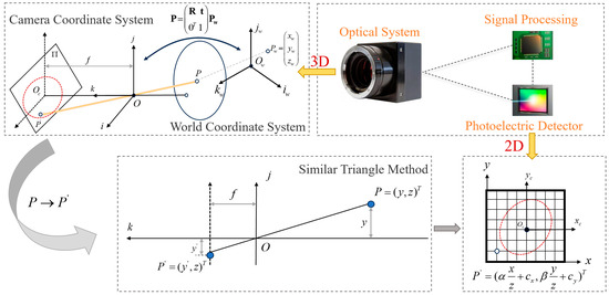
Figure 1. Schematic diagram of space camera imaging principle.

According to the principles of similar triangles in the pinhole camera model, the relationship between the spatial point $P$ and its image point $P^{\prime }$ is established, thus converting the 3D spatial point into a 2D plane image point. Let $s$ be the depth scale factor of the camera, and $K$ be the camera’s intrinsic matrix, with the 2D point coordinates $P^{\prime }=\left(x_c,y_c\right)$ being transformed as follows:

$$s\left[\begin{array}{l}{x}_c\\ y_c\\ 1\end{array}\right]=K\left[\begin{array}{l}R t\\ 0^T 1\end{array}\right]\left[\begin{array}{l}{X}_w\\ Y_w\\ Z_w\\ 1\end{array}\right]$$

(2)

Quaternions provide an alternative representation for describing rotational processes, typically expressed as $q=[q_w,q_x,q_y,q_z]$, with the formula as follows:

$$R=\left[\begin{array}{c}1-2\left(q_y^2+q_z^2\right) 2\left(q_x{q}_y-q_w{q}_z\right) 2\left(q_x{q}_z+q_w{q}_y\right)\\ 2\left(q_x{q}_y+q_w{q}_z\right) 1-2\left(q_x^2+q_z^2\right) 2\left(q_y{q}_z-q_w{q}_x\right)\\ 2\left(q_x{q}_z-q_w{q}_y\right) 2\left(q_y{q}_z+q_w{q}_x\right) 1-2\left(q_x^2+q_y^2\right)\end{array}\right]$$

(3)

The actual space imaging mechanism includes both geometric and radiometric components. The former determines the geometric correspondence of points on the satellite’s surface in 3D space projected onto the image plane coordinate system. The latter determines the brightness and RGB color of the point in the image, or the grayscale value in the case of grayscale images. In a vacuum environment, radiance remains constant along the direction of light, a physical characteristic that makes ray tracing an essential technique for space-based simulation imaging.

This study begins by examining the operational modalities of optical observation satellite platforms, focusing on the geometric constraints between the sun, the observation satellite platform, and space objects. It emphasizes a light field fitting method based on HOSH and integrates the BRDF to calculate the multiple optical scattering characteristic of satellite surface materials. This approach simulates a realistic space environment, significantly enhancing the computational precision and rendering quality of the satellite optical simulation image generation model.

2.2. Geometric and Radiative Rendering Pipeline

For two categories of space optical observation operational modes, this study designs a comprehensive simulation workflow, including both geometric and radiative rendering pipelines as shown in Figure 2. Initially, the camera’s focal length, image resolution, and sensor size are set. Positions and velocities of the sun, target, and platform in the J2000 coordinate system are computed from the dynamic model. Subsequently, local geometric information is extracted from the OBJ format 3D models and vertex data are input. Vertex shaders are then employed for model matrix transformation and observation projection transformation, converting the local coordinate system of the 3D structure into the world coordinate system. Following this, different components of the satellite undergo level-of-detail subdivision to balance the visual effect of texture details and map it to screen coordinates. Finally, two distinct sampling methods are utilized: RSSF, which leverages the properties of the Fibonacci sequence to distribute sampling points in a spiral pattern on the sphere for uniform coverage; SSPT and total frame count to produce uniform intervals and output geometric parameters, including position, normal, and texture information [18].

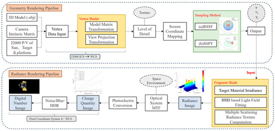
Figure 2. The integrated approach of geometric and radiative rendering pipelines in generating satellite optical images.

The geometric rendering pipeline primarily calculates the coordinate transformations, attitude matrices, vertex data, and sampling results of space objects. These geometric parameters are then input into the radiative rendering pipeline. Initially, fragment shaders are used to select appropriate materials for the target’s components, compute irradiance, and fit the light field using HOSH while simultaneously calculating the radiance texture data from multiple scattering, and generating a radiance image. Subsequently, in conjunction with the actual space environment conditions such as temperature, vacuum, radiation, and microgravity, the MTF of the optical camera is simulated to describe the optical system’s response capability to different spatial frequencies. Following this, a photoelectric conversion is performed, converting radiance into charge counts to obtain a charge quantity image. Finally, the process yields a DN value image with world coordinates transformed to pixel coordinates.

2.3. Fitting the Light Field Distribution Using HOSH

In space, parallel sunlight often predominates, significantly influencing the optical properties of satellite surfaces. However, there is also light reflected from very distant celestial bodies, which can be approximated as area light. For satellites operating over extended periods, the influence of area light on surface materials cannot be overlooked. Consequently, this study proposes a light field fitting method based on HOSH and multiple scattering theory. This method approximates the light sources in the real space environment as parallel light emitted by the sun and area light reflected from distant celestial bodies, incorporating complex scattering effects as one of the influencing factors. Given the radiative mechanisms of spatial optical imaging, accurate simulation of real space environment lighting is crucial for the generation of optical image simulations [19].

In analyzing the optical characteristics of space objects and their background detection under lighting constraints, it is evident that when an object is in a sunlit region, its visible light radiation primarily originates from the reflection of parallel sunlight on the object, where $0<\alpha <\beta <\pi$ and $\cos \alpha >{\displaystyle \frac{u\cdot d}{\left|\right|u\left|\right|\cdot \left|\right|d\left|\right|}}$ hold. The intensity of this reflection is closely related to the angle between the observation line of sight and the sunlight, as illustrated in Figure 3.

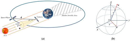
Figure 3. Schematic Diagram of the Light Field Distribution of a Space Object. (a) depicts the scenario in which the object is located within the sunlit visible region. The gray shaded area indicates the Earth-obscured invisible area, while the yellow cone signifies the Line of Sight (LOS). The vector $u$ denotes the distance from the observation platform to the Sun, and $d$ represents the distance vector between the camera and the observed target, with the angle between them labeled as $\beta$. Furthermore, $\alpha$ is defined as the sum of the Sun’s apparent radius and the light scattering angle (a non-negative acute angle). (b) is a polar coordinate diagram of the observation line of sight based on the HOSH.

Spherical harmonics, as detailed by, constitute a set of orthogonal basis functions defined on the unit sphere, exhibiting mathematical properties such as orthogonality and completeness [20]. The expansion of any function in terms of spherical harmonics can be truncated to a finite number of terms, analogous to the role of Fourier series in periodic functions, thereby facilitating a lower-dimensional representation. Consider the light field $L(\theta ,\varphi )$, which can be expressed as a linear combination of HOSH, as depicted in Figure 4.

$$L(\theta ,\varphi )=\sum _{l=0}^{L_{\max }}\sum _{m=-l}^l{c}_l^m{N}_l^m{P}_l^m(\cos \theta )e^{im\varphi }$$

(4)

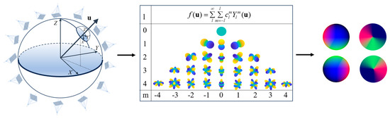
Figure 4. Distribution of the light field based on HOSH, assuming $r=1$, and considering computational resources, we yield $L_{\mathrm{m}\mathrm{a}\mathrm{x}}=4$.

Here, $c_l^m$ denotes the spherical harmonic coefficients, representing the projection of the light field onto the spherical harmonic basis, with $L_{\mathrm{m}\mathrm{a}\mathrm{x}}$ being the maximum order, $l\ge 0$, $-l\le m\le l$ [21].

$Y_l^m$ represents the spherical harmonics, where $l$ is the order and $m$ is the degree. As the order of spherical harmonics increases, HOSH can approximate more complex distributions of the light field across multiple directions; $P_l^m$ is the associated Legendre polynomial; $N_l^m$ is a normalization constant; $\theta$ and $\varphi$ are the elevation and azimuth angles, respectively, measured from the positive $z$-axis and the positive $x$-axis. By definition, $\theta \in [0, \pi ]$, $\varphi \in [0, 2\pi ]$. The conversion relationship between the elevation angle $\theta$, azimuth angle $\varphi$, and line-of-sight direction $d=(x,y,z)$ is as follows.

$$\left\{\begin{array}{c}z=r\cos (\theta )\\ y=r\sin (\theta )\sin (\varphi )\\ x=r\sin (\theta )\cos (\varphi )\end{array}\right.$$

(5)

Normalization constants $N_l^m$ are commonly employed to ensure the orthogonality of spherical harmonics, and $P_l^m\left(x\right)$ is defined as follows:

$$\left\{\begin{array}{l}{P}_l^m(x)=(-1{)}^m{\left(1-x^2\right)}^{m/2}{\displaystyle \frac{d^m}{d{x}^m}}{P}_l(x)\\ {\int }_{-1}^1{P}_l^m(x)P_{l^{\prime }}^m(x)dx={\displaystyle \frac{2}{2l+1}}{\displaystyle \frac{(l+m)!}{(l-m)!}}{\delta }_{l{l}^{\prime }}\\ N_l^m=\sqrt{{\displaystyle \frac{2l+1}{4\pi }}{\displaystyle \frac{(l-m)!}{(l+m)!}}}\\ {\int }_{\mathsf{\Omega }}{Y}_l^m(\theta ,\varphi )Y_{l^{\prime }}^{m^{\prime }}(\theta ,\varphi )d\mathsf{\Omega }={\delta }_{l{l}^{\prime }}{\delta }_{m{m}^{\prime }}\end{array}\right.$$

(6)

where ${\delta }_{l{l}^{\prime }}$ is the Kronecker $\delta$ function, and $d\mathsf{\Omega }=\mathrm{s}\mathrm{i}\mathrm{n}\theta d\theta d\varphi$ is the differential solid angle, ensuring that the spherical harmonics meet the normalization condition.

The real-world space environment light field $L(\theta ,\varphi )$ comprises a combination of parallel sunlight emitted by the sun and diffuse light reflected from distant celestial bodies. The interaction between these sources is not merely a linear superposition but is also affected by distance attenuation and occlusion effects, which collectively determine the actual intensity variations in light during propagation.

• Sunlight as Parallel Light:

Sunlight can be considered a directional light source, approximated by the Dirac delta function, as follows:

$$L_{sun}(\theta ,\varphi )=\delta \left(\theta -{\theta }_{sun},\varphi -{\varphi }_{sun}\right)$$

(7)

where ${\theta }_s$ and ${\varphi }_s$ are the incident directions of the sunlight, which, when expanded using HOSH, yields the solar light spherical harmonic coefficients $c_l^m$.

2.

Light from Distant Celestial Bodies:

Light reflected from distant celestial bodies can be considered as an area light source, and its light field can be represented as follows:

$$L_{ast}(\theta ,\varphi )=\sum _{l=0}^{L_{\max }}\sum _{m=-l}^l{c}_l^{m,ast}{Y}_l^m(\theta ,\varphi )$$

(8)

where $c_l^{m,ast}$ are the spherical harmonic coefficients for the celestial reflected light.

In summary, combining the effects of superposition of light fields, distance attenuation, and occlusion, and assuming an average propagation distance of $d_{ast}$ for light from distant celestial bodies, $V\left(\omega \right)$ is the visibility function of the light direction $\omega$, the model for the light field in a space environment can be represented as follows:

$$L_t(\theta ,\varphi )=L_{sun}(\theta ,\varphi )+L_{ast}(\theta ,\varphi )\cdot {\displaystyle \frac{1}{d_{ast}^2}}\cdot V_{ast}(\omega )$$

(9)

3. Optical Scattering Model of Space Objects

The interaction of light with objects typically results in a shaded point along with geometric information about the surface element at that point. Therefore, it is necessary to compute the illuminance at this point. This computation involves understanding the geometric and radiometric distribution of light across different spatial operational modes. The BRDF is defined as the ratio of reflected radiance to incident irradiance and is widely used in optical engineering of space objects.

3.1. Experiment of Spectral Reflectance

The typical materials of space objects can be categorized into four primary classes based on their functional applications: alloys, cladding materials, solar sail panels, and thermal control coatings, along with replaceable payloads. Depending on the BRDF characteristics of each material, they can be broadly classified into two types: materials that primarily exhibit specular reflection and those that primarily exhibit diffuse reflection. Specular reflectance materials predominantly include cladding materials, solar panels, Optical Solar Reflectors (OSRs), and certain polished alloys; diffuse reflectance materials mainly consist of various thermal control coating materials, typically including organic spray paints, Carbon Fiber Reinforced Polymers, and some oxidized alloys.

In preliminary work, the team conducted spectral reflectance measurements on sixteen commonly used materials of space objects, across the wavelength range of 400–1800 nm, using the FieldSpec@4 as the spectral detector, as depicted in Figure 5. The REFLET 180S is an automated measurement system developed by Light Tec for measuring the scattering BRDF of sample materials with an angular control precision of 0.01°. It also provides a stable light source and a dark background, which justifies its selection as both the light source and the turntable control system. Given the intrinsic spectral range of the built-in light source in the REFLET 180S, the experimental measurement wavelength was set between 400–1800 nm. Through the spectral reflectance experiment, the diffuse reflection coefficient, specular reflection coefficient, and specular reflection index of the incident light on the satellite surface materials can be obtained [22].

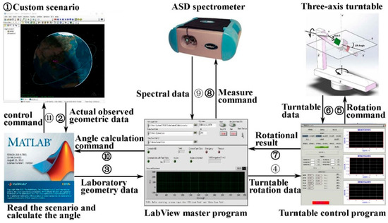
Figure 5. Experimental model of spectral reflectance. This figure includes the experimental measurement system, primarily composed of the REFLET 180S from Light Tec, France, and the FieldSpec@4 fiber optic spectrometer from Analytical Spectral Devices, Boulder, CO, USA. Through the LabVIEW (2024 Q3) master control software, the fully automated spectral data measurement is achieved, enabling the automatic rotation of the turntable and the automatic measurement by the ASD [23].

Spectral reflectance models can be categorized into four types: directional-directional reflectance, hemispherical-directional reflectance, directional-hemispherical reflectance, and hemispherical-hemispherical reflectance. In typical space-based scenarios, the focus is on how incident light from a specific direction reflects off the surface of space objects and enters the camera along a specific exit path. Therefore, directional-directional reflectance models are typically used in simulation imaging. Integrating the directional-directional spectral reflectance into the BRDF enhances the accuracy of modeling the reflective behavior of space object surfaces, thereby providing a more reliable basis for the optical camera’s simulation of imaging space objects [24].

3.2. An Improved Phong Model

The geometric relationship between the Sun, the target satellite, and the detection system is illustrated in Figure 6. It is assumed that the surface of the target satellite comprises numerous minuscule surface elements. The BRDF of a surface element $dA$ for solar radiation in the visible spectrum is denoted by $f_r$. The unit normal vector of $dA$ is represented by $\mathit{n}$, the unit vector from $dA$ to the Sun is ${\mathit{\omega }}_{\mathit{i}}$, and the unit vector from $dA$ to the detection system is ${\mathit{\omega }}_{\mathit{r}}$. The angle between the projections ${\mathit{\omega }}_{\mathit{i}}$ and ${\mathit{\omega }}_{\mathit{r}}$ on the surface element is $\psi$, the angle between n and ${\mathit{\omega }}_{\mathit{i}}$ is ${\theta }_{\mathrm{i}}$, and the angle between n and ${\mathit{\omega }}_{\mathit{r}}$ is ${\theta }_{\mathrm{r}}$.

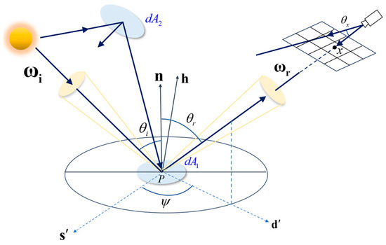
Figure 6. Schematic diagram of a multi-modal imaging physical simulation model based on ray tracing algorithms.

According to the diagram,

$$\left\{\begin{array}{c}\cos {\theta }_{\mathrm{i}}=\mathbf{n}\cdot {\mathbf{\omega }}_{\mathbf{i}}, \cos \theta =n\cdot {\omega }_r\\ \cos \psi =(n\times {\mathbf{\omega }}_{\mathbf{i}}\times n)\cdot (n\times {\omega }_r\times n)\end{array}\right.$$

(10)

The solar flux $d{\Phi }_{\mathrm{i}}$ and the irradiance $d{E}_{\mathrm{i}}$ received by the surface element $dA$ are given by

$$\left\{\begin{array}{l}d{\mathrm{\Phi }}_{\mathrm{i}}=E_{\mathrm{sun}}\cos {\theta }_{\mathrm{i}}dA\\ d{E}_{\mathrm{i}}={\displaystyle \frac{d{\mathrm{\Phi }}_{\mathrm{i}}}{dA}}=E_{\mathrm{sun}}\cos {\theta }_{\mathrm{i}}\end{array}\right.$$

(11)

Reflectance is defined as the ratio of the energy reflected by an object to the incident energy. The term “spectral reflectance” refers to the reflectance curve of an object measured across a continuum of wavelengths. Consequently, the BRDF quantifies factors such as the roughness of the material’s surface, dielectric constant, radiative wavelength, and polarization [25].

The radiated flux $d{\Phi }_{\mathrm{r}}$ from the surface element $dA$ in the direction ${\mathit{\omega }}_{\mathit{r}}$, along with its radiance $d{L}_{\mathrm{r}}$ and intensity $I_{\mathrm{r}},$ within a unit solid angle $d{\omega }_{\mathrm{r}}$ are specified. The BRDF of the target surface material under solar illumination conditions, which depends solely on ${\theta }_{\mathrm{i}}$ and $\theta$, can be derived from the definition of BRDF as

$$I_{\mathrm{r}}={\displaystyle \frac{d{\mathrm{\Phi }}_{\mathrm{r}}}{d{\omega }_r}}=E_{\mathrm{sun}}{f}_{\mathrm{r}}({\theta }_{\mathrm{i}},\theta )\cos {\theta }_{\mathrm{i}}\cos \theta dA$$

(12)

The flux $d{\Phi }_{\mathrm{d}}$ received by the entrance pupil element $ds$ of the detection system in the direction ${\mathit{\omega }}_{\mathit{r}}$ from the surface element $dA$ is as follows:

$$d{\mathrm{\Phi }}_{\mathrm{d}}=I_{\mathrm{r}}d\mathrm{\Omega }=E_{\mathrm{sun}}{f}_{\mathrm{r}}({\theta }_{\mathrm{i}},\theta )\cos {\theta }_{\mathrm{i}}\cos \theta dA\cdot {\displaystyle \frac{ds}{R_1^2}}$$

(13)

where $d\Omega$ represents the solid angle subtended by the entrance pupil element $ds$.

Let $S_0$ denote the area of the detection system’s entrance pupil. Consequently, the total flux received by the entire detection system from the target is

$${\mathrm{\Phi }}_{\mathrm{d}}={\displaystyle \underset{S_0}{\int }{\displaystyle \underset{A}{\int }{E}_{\mathrm{sun}}{f}_{\mathrm{r}}({\theta }_{\mathrm{i}},\theta )\cos {\theta }_{\mathrm{i}}\cos \theta dA\frac{ds}{R_1^2}}}$$

(14)

Typically, the distance R₁ significantly exceeds the radius of the entrance pupil. Thus, the orientations of each entrance pupil element relative to the target are consistent. Assuming the effective operational range of the detection system is from 450 nm to 900 nm, through integral computation, the solar irradiance in the visible spectrum can be determined to be 647.7 W/m², and the total irradiance received by the detection system is

$$E_{\mathrm{target}}={\displaystyle \frac{{\mathrm{\Phi }}_{\mathrm{d}}}{S_0}}={\displaystyle \frac{E_{\mathrm{sun}}}{R_1^2}}\cdot \left({\displaystyle {\int }_A{f}_{\mathrm{r}}({\theta }_{\mathrm{i}},\theta )\cos {\theta }_{\mathrm{i}}\cos \theta dA}\right)$$

(15)

Both the main covering material of space objects and solar panels generally exhibit both incoherent and coherent scattering components. For precise calculation of the light scattering properties of space objects, it is essential to establish a model of the diffuse and specular reflection characteristics of surface materials of space objects. Given the additive nature of light, assuming that the scattering properties of the target surface are wavelength-independent, diffuse and specular reflections are considered separately based on the above assumption.

The Phong model is a widely utilized simplified lighting model in computer graphics [26]. Its most basic form accounts solely for the reflection of direct light from a light source by an object. By representing a four-dimensional vector in polar coordinates, the simplified Phong model can be expressed as follows.

$$f=k_{\mathrm{d}}+k_{\mathrm{s}}{\displaystyle \frac{{\cos }^g\beta }{{\cos }^a{\theta }_{\mathrm{i}}}}$$

(16)

Here, $k_d$ represents the diffuse reflection coefficient for incident light, $k_s$ the specular reflection coefficient. To address the challenge of describing the Fresnel reflection phenomenon, this study transforms the distribution model of the light field fitted with HOSH based on actual solar illumination conditions to align with the physical characteristics of BRDF as follows [27]. An improved Phong model is proposed, as shown in the following equation.

$$f_{\mathrm{r}}=k_{\mathrm{d}}\cos {\theta }_{\mathrm{i}}+k_{\mathrm{s}}{\displaystyle \frac{{\cos }^g\beta }{{\cos }^a{\theta }_{\mathrm{i}}}}\exp [-b{(1-\cos \beta )}^{1/\pi }]$$

(17)

Here, $g$ the gloss exponent, primarily describing the sharpness of specular reflections, typically related to the roughness $\alpha$ in the GGX microsurface distribution model. $\beta$ represents the angle between the observation direction and the direction opposite to the incident light. $a>0$, which is used to adjust the intensity of the Fresnel reflection. $b>0$ adjusts the rate of increase or decrease in the specular reflection component. The angle $\phi$ is between $\mathit{n}$ and vector ${\mathit{d}}^{\prime }$, where ${\mathit{d}}^{\prime }=({\mathit{\omega }}_{\mathit{r}}+{\mathit{\omega }}_{\mathit{i}})/\left|{\mathit{\omega }}_{\mathit{r}}+{\mathit{\omega }}_{\mathit{i}}\right|$. Based on the principle of high-order cosine, the modified specular reflection term enables the adjustment of the azimuthal peak increase rate for different materials. Additionally, the modified diffuse reflection term enhances the fitting accuracy at extreme incident angles, while the introduced exponential term provides control over the increase or decrease rate of the specular component in the fitted image.

In summary, assuming the direction of incident light reflected by satellite surface materials is ${\mathit{\omega }}_{\mathit{i}}$ and the direction of reflected light is ${\mathit{\omega }}_{\mathit{r}}$, with the normal of the material surface denoted by $\mathit{n}$, and ${\theta }_i=\mathrm{a}\mathrm{r}\mathrm{c}\mathrm{c}\mathrm{o}\mathrm{s}\left({\mathit{\omega }}_{\mathit{i}}\cdot \mathit{n}\right)$. Based on Equations (9) and (17), a comprehensive model can be established between the satellite surface materials and the light source as follows:

$$L_{out}\left({\omega }_r\right)={{\displaystyle \int }}_{\mathsf{\Omega }}{f}_r\left({\omega }_i,{\omega }_r\right)\cdot L_t\left({\theta }_i,\varphi \right)\cdot \cos {\theta }_i\cdot dA$$

(18)

3.3. Satellite Surface Materials

In order to facilitate experimental design, this study categorizes the structure of satellites into four main components based on the functional applications of typical materials used in space objects: the satellite body, solar sail panels, payload, and connecting components.

The satellite body, serving as the foundational structure, provides a platform and support for other components, primarily utilizing high-strength, lightweight metal materials. Its surface is typically covered with multi-layer insulation materials, predominantly high-performance polymeric materials such as polyimide (PI), enhanced by thermal control coatings in the form of white paint or textured panels. The solar sail panels, acting as the energy supply system, commonly employ monocrystalline or polycrystalline silicon solar cells, or third-generation gallium arsenide solar cells, with the rear side featuring composite aluminum honeycomb panels or flexible solar substrates. The payload, critical for mission-specific tasks, often incorporates surfaces made from carbon fiber-reinforced composites and alloy materials; in space surveillance missions, optical payloads utilize fused silica glass lenses and carbon fiber-reinforced composite lens barrels, enveloped in multi-layer black wrinkled coatings to absorb light and mitigate solar radiation and temperature variations that could damage optical systems. Connecting components, essential for transferring mechanical loads and signals, frequently feature materials such as titanium alloys or black high-temperature alloys, as seen in hinges and nuts linking the solar sail panels.

This study predominantly utilizes a physically based rendering model to simulate the interactions between materials and light sources. This model integrates various physical phenomena, including reflection, refraction, diffuse reflection, and subsurface scattering. The material properties are described through parameters such as metallicity, roughness, index of refraction (IOR), and Alpha, which are correlated with related parameters as depicted in Equation (17).

• Metallic:

The concept of metallicity (M) is utilized to describe the metallic attributes of a material, with values $M\in [0,1]$. The relationship between $M$ and $k_s$ and $k_d$ can be expressed as follows:

$$\left\{\begin{array}{l}{k}_d=(1-M)\cdot RGB\\ k_s=M\cdot RGB+(1-M)\cdot F_0\end{array}\right.$$

(19)

Here, the RGB representation is employed to denote the values of different color channels using hexadecimal, where each channel ranges from 0 to 255. Typically, a three-character representation is used to indicate the base color of the material. The Fresnel reflectance at normal incidence, denoted as $F_0$, is characteristically higher for metallic materials and lower for non-metallic materials [28]. For instance, aluminum has an $F_0$ of 0.91.

2.

Roughness:

Roughness $R$ quantifies the degree of surface roughness of a material, with values $R\in [0,1]$. Surfaces with higher roughness enhance the reflected energy due to multiple scattering events. This study employs Schlick’s GGX model, setting $k=\alpha /2$ [29]. Based on the directional-hemispherical spectral reflectance model, this describes the phenomena of multiple surface scattering [30]. Assuming α represents the roughness parameter, where masking and shadowing effects are considered independent, and known that $\alpha =R^2$, the mapping relationship between roughness and the microsurface distribution function $D\left({\omega }_h\right)$ and the geometric attenuation function $G\left({\omega }_i,{\omega }_r\right)$ is as follows:

$$\left\{\begin{array}{l}D\left({\omega }_h\right)={\displaystyle \frac{{\alpha }^2}{\pi {({(\mathbf{n}·h)}^2({\alpha }^2-1)+1)}^2}}\\ G\left({\omega }_r\right)={\displaystyle \frac{\mathbf{n}·w_r}{(\mathbf{n}·{\omega }_r)(1-k)+k}}\\ k={\displaystyle \frac{{(R+1)}^2}{8}}\end{array}\right.$$

(20)

Due to the complexity of target shapes, the calculation process must consider not only whether each small surface element can be illuminated by sunlight but also whether it is obstructed by other elements, addressing the issue of occlusion. In the equation above, $\mathit{h}$ represents the halfway vector, describing a unit vector in the direction of the normals of individual micro-surface elements, $\mathit{h}={\displaystyle \frac{{\omega }_i+{\omega }_r}{\left|\right|{\omega }_i+{\omega }_r\left|\right|}}$. The geometric attenuation function $G\left({\mathit{\omega }}_{\mathit{r}}\right)$ corrects for the loss of light energy, ensuring that the rendering model adheres to the law of energy conservation and enhances the realism of optical simulations in space environments.

3.

IOR:

IOR describes the material’s ability to refract light and its mapping relationship with the Fresnel reflectance $F_0$ is as follows:

$$F_0={\left({\displaystyle \frac{IOR-1}{IOR+1}}\right)}^2$$

(21)

4.

Alpha:

Alpha parameter indicates the transparency of a material, with values $Alpha\in [0,1]$. A value of 1 indicates complete opacity, whereas a value of 0 indicates total transparency.

Metallicity characterizes the electronic structure of surface materials, while roughness quantifies the geometric disorder at the surface. IOR fundamentally governs the strength of light-matter interactions, and transparency embodies the statistical characterization of photon penetration depth within dielectric media. The co-design of these four parameters establishes a scale-bridging physical mapping that spans from quantum-scale electronic states to macroscopic radiative fields. By rigorously constraining light-surface interactions through physically measurable and derivable quantities, this framework achieves a closed-loop integration, transitioning from laboratory-based semi-physical measurements in controlled darkroom environments to synthetic renderings. It provides a unified model for characterizing complex, spatially varying optical phenomena, ensuring both theoretical precision and practical utility.

4. Simulation Results

4.1. Simulation Scenarios

At present, the majority of satellites employ a three-axis stabilized attitude control method, wherein all three coordinate axes are fixed in position and orientation relative to inertial space. This stabilization allows for the utilization of specific components, such as optical devices, to align with the observed space objects. In space-based observations, both the observational platform and the target generally orbit according to predefined trajectories, exhibiting certain degrees of relative motion. This study conducts space-based imaging simulation research based on two classical space motion scenarios: fly-around and fly-by observations. Through dynamic calculations, the orbital information of both the in-orbit platform and the space objects under observation is determined, describing their spatial operational modes and geometric constraints, as illustrated in Figure 7.

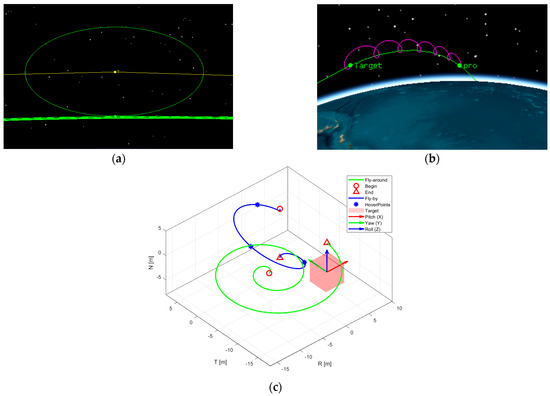
Figure 7. Spatial operational modes and sequential sampling method. (a) corresponds to the fly-around spatial operational mode; (b) corresponds to the fly-by spatial operational mode; (c) represents the sequential sampling method based on a predefined trajectory. The green solid line corresponds to mode (a) and the blue solid line to mode (b). Both trajectories illustrate the numerical integration process from start to finish. The blue “*” symbols denote hovering observation points during the approach, and the red boxes represent the axis-aligned bounding box (AABB) of the target. The coordinate system, centered within the box, represents the satellite body-fixed attitude coordinate system, displaying roll, elevation angle, and azimuth angle.

It is crucial to note that the observing satellite, in both spatial operational modes, must satisfy conditions of geometric visibility and optical visibility to facilitate visual analysis under space-based observations. Geometric visibility refers to the mutual visibility between the observing satellite and the space objects, unobstructed by Earth or other spatial bodies. Optical visibility denotes that the space objects are not within the Earth’s shadow region, the optical lens is not directed towards the Sun, and the conditions are favorable for observation with backlighting [31]. The orbital parameters of the space objects and the detection satellite that meet the aforementioned visibility conditions are outlined in Table 1. Initially, the orbital elements (OE) for both the space objects and the observing satellite are set. Subsequently, the terminal OEs for the observing satellite are designated for fly-by (OE1) and fly-around (OE2) scenarios, utilizing the Runge–Kutta numerical integration method with a timestep of 1 s. The relative attitude (relative pose) between the target and the camera is defined in the RTN coordinate system. The camera’s optical axis (Z-axis) initially aligns with the negative orbital direction (-T), and the X-axis aligns with the normal direction (N). Through attitude control, the camera’s optical axis consistently points towards the T-axis. During the trajectory simulation process, the target maintains an approximately constant relative position to the camera in OE1, while in OE2, the camera follows a spiral trajectory approaching the target.

Table 1. Orbital parameters for space objects and detection satellite in different operational modes.

Orbital Parameters	Initial OE for Space Objects	Initial OE for Observing Satellite	Terminal OE for Observing Satellite (Fly-By)	Terminal OE for Observing Satellite (Fly-Around)
$a \left(\mathrm{k}\mathrm{m}\right)$	6878.137	6878.137	6873.136077	6861.380356
$e$	0.0000	0.0000	0.000515	0.001317
$i \left(°\right)$	98.5	98.5	98.506	98.512
$\Omega (°)$	360	360	1.115	0.545
$\omega (°)$	0	0	179.268	292.901
$F$	0	30	147.547	172.686

In the simulation experiments, two distinct sampling methods were designed to simulate geometric constraints from an attitude dynamics perspective. These include SSPT and RSSF. SSPT, as depicted in Figure 7c, primarily simulates two typical spatial operational modes: fly-around and fly-by. The method accounts for relative motion and geometric visibility relationships and completes the optical imaging computation process through a radiative rendering pipeline.

In addition, this study introduces a second sampling method, RSSF, as shown in Figure 8. A random seed number of 5 was used. The blue great circles are the intersections of different planes passing through the sphere’s center with the corresponding spherical surface. Theoretically, the number of such great circles is infinite, hence the infinite number of gray points representing random camera perspectives generated by the spherical Fibonacci function. RSSF enhances the automation speed of rendering, allowing for the rapid generation of a vast number of images in a short period, covering as many 3D perspectives as possible. This method is particularly suitable for subsequent research on algorithms such as attitude estimation based on deep learning.

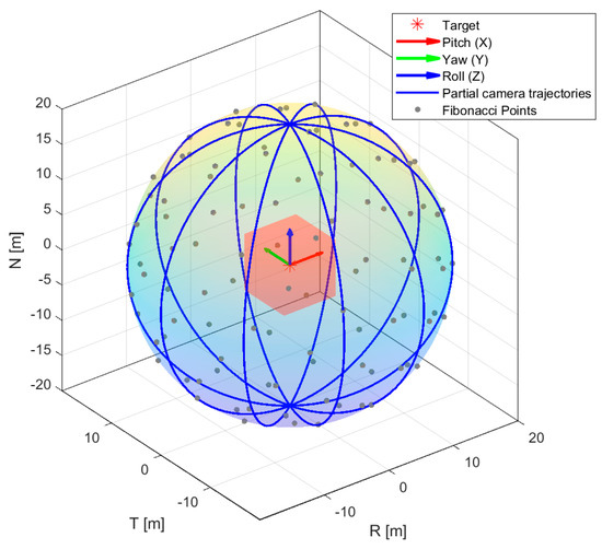
Figure 8. RSSF. With a random seed count of 5, the gray points represent camera perspectives in physical space and random sampling points generated by the Fibonacci function in geometric space. The red box indicates the target’s AABB, and the coordinate system centered within this box is the satellite body−fixed attitude coordinate system, showcasing roll, elevation angle, and azimuth angle.

4.2. Experimental Parameters

• Camera Parameters:

A space camera is an imaging system characterized by unique features such as high resolution, long-distance observation, and adaptability to extreme environments. Typically, different visual tasks require varying pixel sizes for the target. Taking space target recognition as an example, the minimum pixel requirement for the target is approximately 50 pixels. This simulation experiment models a compact coaxial detection optical system with a large field of view (FOV) for spaceborne global imaging. The design is fine-tuned based on the physical parameters of the CCD231-84 E2V photodetector (Teledyne Technologie, Thousand Oaks, CA, USA). As shown in Table 2, the camera features a pixel array of 4096 × 4112, with a pixel size of 15 μm × 15 μm. The projection method is perspective projection, and the target has a diameter of approximately 5 m. Based on a dual-mode design concept, the system operates in a high-resolution mode with a focal length of $f_1=3m$ and a FOV of approximately 2°, and in a wide-FOV mode with a focal length of $f_2=0.7m$ and a FOV of approximately 10°. According to Equation (9), the simulation is expected to achieve effective detection of stars up to the 9th magnitude.

Table 2. Imaging simulation parameters of the lens and detector under different scenarios and operational modes.

Optical System Design Index		Value
Sensor size/mm × mm		61.44 × 61.68
Wavelength/nm		450–800
Number of pixels		4096 × 4112
Pixel size/μm × μm		15 × 15
Entrance pupil/mm		280
Diameter of Target/m		5
Orbital Altitude of Target/km		500
FOV/degree	High-resolution Mode	2
	Wide-FOV Mode	10
Focal Length/m	High-resolution Mode	3
	Wide-FOV Mode	0.7

2.

Satellite Surface Material Parameters:

The experimental setup involves the calibration of materials based on their BRDF properties, adopting distinct calibration bodies for diffuse and specular reflection types. Incidence angle measurements are taken at intervals of 2 degrees to accommodate these material properties. As illustrated in Figure 9, the data presented represents the average spectral reflectance measurements of 16 different materials for spatial targets.

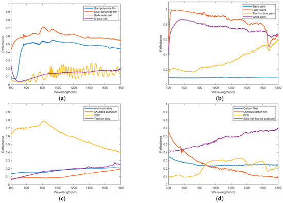
Figure 9. The spectral response curves of 16 materials for spatial objects are depicted as follows: (a) encapsulates materials and solar cells; (b) represents various types of paint; (c) includes alloys and OSR; (d) showcases carbon fiber, carbonized films, Printed Circuit Boards, and battery substrates.

Using the pertinent measurement data, the BRDF parameters of the satellite surface materials are fitted and calculated using Equations (18)–(20) to generate the corresponding optical characteristic simulation parameters. These parameters include metallicity, roughness, IOR, and Alpha, as detailed in Table 3.

Table 3. Typical material and simulation parameters for space objects.

Material	Component Information	Typical Materials	(M, R, IOR, and Alpha)
Alloy	Satellite Main Body Structure	Brushed Metal Panel	(1, 0.3, 1.45, 1)
	Fuel Tank	Titanium Alloy	(1, 0.3, 1.45, 1)
	Connection Components	Black Beryllium Alloy	(1, 0.5, 1.45, 1)
	Hinge	Nickel-based High-Temperature Alloy	(1, 1, 1.45, 1)
Cladding Materials	Multilayer Insulation Material MLI	PI Film (gold, silver, black)	(1, 0.3, 1.45, 1)
	Support Structures	Black Carbon Fiber Composite Substrate	(0, 0.5, 1.45, 1)
Thermal Control Coatings	Sprayed Thermal Insulation Material	Organic Paints (organic white paint, black paint, epoxy paint, titanium blue paint)	(1, 1, 1.45, 1)
	Radiation-Texture Coating	Silica-based Coating	(0, 0.5, 1.5, 1)
	Black Wrinkle Paint	Epoxy Resin	(0, 0.6, 1.45, 1)
Solar Sail Panels	Solar Sail Panels	GaAs/Si	(1, 0.3, 1.45, 1)
Replaceable Payloads	Optical Lenses	OSR	(0.1, 0.85, 1.5, 1)

4.3. Texture Features

The 3D model of the IceSat-2, as illustrated in Figure 10, is depicted in its initial attitude, defined by azimuth, elevation, and roll angles set at zero, consequently represented by the quaternion $[q_w,q_x,q_y,q_z]=[1, 0, 0, 0]$. The satellite is composed of multiple modules and components, including optical lenses, textured coatings, silver-clad sheets, and solar sail panels, among other parts totaling thirteen. The main body resembles a cylindrical shape; however, due to the installation of devices varying in specifications and functionalities, the surface of the hull exhibits varying degrees of protrusions, indentations, and structures designed for connection, heat dissipation, and insulation [32].

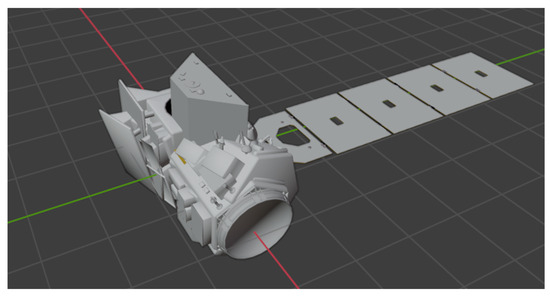
Figure 10. 3D model in initial attitude.

Based on the settings of typical materials’ parameters for space objects, it is possible to obtain detailed reflections of light sources on different surface materials. It is evident that there is a clear contrast in light intensity, indicating that the simulation of light sources and reproduction of surface materials based on the BRDF and HOSH have achieved a satisfactory level of accuracy. This approach approximates the optical characteristics of space objects closely to real space conditions, ultimately producing high-resolution spatial optical images.

4.4. Comparative Analysis

The ablation experiments for each proposed module are summarized in Table 4, with all metrics averaged. The results indicate that the improved Phong model significantly outperforms the original in terms of MSE, PSNR, and angular error, demonstrating superior capability in characterizing the optical scattering properties of complex surfaces. Additionally, 4th SH surpass 3rd SH in fitting accuracy, edge representation, and directional lighting adaptability, capturing higher-frequency details to more precisely describe light field distributions. This approach reduces edge artifacts caused by low-order approximations and enhances rendering realism.

Table 4. Analysis of ablation experiment metrics.

Model	$\mathbf{M}\mathbf{S}\mathbf{E}$	$\mathbf{P}\mathbf{S}\mathbf{N}\mathbf{R} \left(\mathit{d}\mathit{B}\right)$	$\mathbf{T}\mathbf{i}\mathbf{m}\mathbf{e} (\mathit{s}/\mathit{F}\mathit{r}\mathit{a}\mathit{m}\mathit{e})$	Angular Error/°
Phong + 3rd SH	$1.8\times {10}^{-3}$	32.5	0.53	6.5
Improved Phong + 3rd SH	$6.5\times {10}^{-4}$	42.8	1.65	2.8
Improved Phong + 4th SH	$5.2\times {10}^{-4}$	45.2	2.86	1.2

Partial results obtained through two different sampling methods are illustrated in Figure 11. Besides, Figure 12a–f employ uniform RSSF, whereas Figure 12g–l utilize SSPT, with a rotational angle range from 0° to 360° and an interval of 5° per frame.

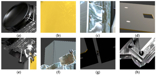
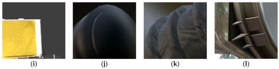
Figure 11. Detailed reflections of light sources on different surface materials. (a) Optical Lenses; (b) Textured Coating; (c) Silver Foil Sheet; (d) Solar Sail Panels; (e) Instrumentation Equipment; (f) Brushed Metal Panel; (g) Hinge; (h) Blach Metal; (i) White Paint; (j) Black Carbon Fiber Composite Substrate; (k) Black Crinkle Coating-Light Absorbing; (l) Telescope Tube.

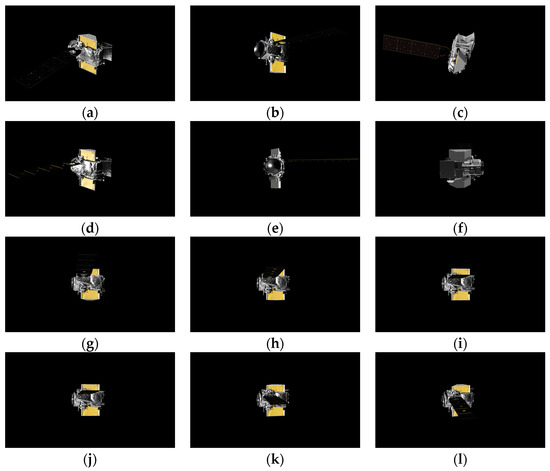
Figure 12. Image datasets, camera, and attitude information under two different sampling methods in the high-resolution operational mode, where (a–f) are based on RSSF and (g–l) are based on SSPT.

Relative to the initial attitude depicted in Figure 10, the quaternions representing the attitudes corresponding to the subset of dataset images in Figure 12a–l are shown in Table 5.

Table 5. Quaternions of the dataset’s partial images relative to the initial attitude.

No.	${\mathit{q}}_{\mathit{w}}$	${\mathit{q}}_{\mathit{x}}$	${\mathit{q}}_{\mathit{y}}$	${\mathit{q}}_{\mathit{z}}$
(a)	0.8281	0.4632	0.1545	0.2768
(b)	0.5836	0.7054	−0.3100	−0.2564
(c)	0.2465	0.7432	0.5904	0.1958
(d)	−0.3380	−0.6189	0.6223	0.3398
(e)	0.4988	0.5466	−0.4968	−0.4534
(f)	0.0177	0.0123	0.5691	0.8203
(g)	0.5991	−0.7997	0.0323	0.0242
(h)	0.6641	−0.7452	0.0454	0.0405
(i)	0.6947	−0.7158	0.0507	0.0492
(j)	0.7239	−0.6852	0.0553	0.0584
(k)	0.7518	−0.6532	0.0592	0.0681
(l)	0.8028	−0.5859	0.0653	0.0895
(g)	0.5991	−0.7997	0.0323	0.0242

Assuming distance units are in km, for different types of space observation missions, datasets at varying relative distances are required for research purposes. During the hovering phase, the distance between the observation platform and the target spacecraft is 100 km, where the satellite typically appears as a small object. In the approaching phase, the relative distances are divided into six intervals: $\left(50,\left.40\right]\right.$, $\left(40,\left.30\right]\right.$, $\left(30,\left.20\right]\right.$, $\left(20,\left.10\right]\right.$, $\left(10,\left.5\right]\right.$, and $\left(5,\left.0.5\right]\right.$. The imaging effects at these distances are illustrated in Figure 13.

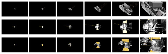
Figure 13. Imaging effects at different relative distances within part of the dataset.

Observations indicate that the target images occupy proportions of 5%, 8%, 12%, 24%, 62%, and 92% across these six distance intervals, respectively. The dataset comprehensively covers all stages of the two space operation modes, with a balanced distribution of images and a high degree of fidelity in replicating the motion states during the approach phase.

Furthermore, as shown in Table 6, this study conducts a comprehensive multi-dimensional comparison between the proposed dataset and existing space object datasets, encompassing aspects such as the number of images, satellite categories, image types (grayscale/color), availability of depth maps, mask maps, 6D pose labels, 3D models, support for physical experiments, and surface texture fidelity. The results demonstrate that the proposed dataset not only provides prior information essential for 3D perception algorithms, including depth, and masks, but also includes ground-truth 3D models for comparative evaluation. Additionally, the high-fidelity surface textures offer enhanced information support for tasks such as pose estimation and 3D reconstruction.

Table 6. Comparison of different space object datasets.

Dataset Types	SPARK [10]	Speed+ [11]	URSO [33]	Swisscube [12]	Minerva-II2 [13]	Ours
Total Number of Images	150 k	15 k	15 k	21 k	20 k	100 k
Category	15	1	2	1	1	5
Color	√	×	√	√	×	√
Depth	×	×	×	×	×	√
Mask	√	×	×	×	√	√
6D Pose	√	√	√	√	√	√
3D Model	√	×	×	√	√	√
Surface Texture Fidelity	×	√	×	×	×	√
Render	simulated	simulated + lab	simulated + lab	simulated	simulated + lab	simulated + lab

5. Discussion

In summary, SSPT is primarily suited for simulating satellites operating in a three-axis stabilized mode relative to the Earth. During the motion, the camera platform consistently points toward the geometric center of the satellite. On the other hand, RSSF ensures image quality by maintaining a near-relative stillness between the satellite and the camera, thereby enabling the rapid simulation of a wide range of relative attitude relationships. These two distinct sampling approaches, respectively, fulfill the dataset requirements for different algorithms in space-based scenarios.

In addition, the optical image simulation dataset of space targets can meet the requirements of various visual tasks and plays a significant role in further research. Based on the characteristics of the simulated images, as shown in Table 7, the following conclusions can be drawn.

Table 7. Quantitative analysis of imaging results and evaluation of recognition capability.

Observation Distance	Operational Mode	Spatial Resolution	Satellite Size in Pixels	Recognition Capability
5 km	High-resolution Mode	0.025 m	200	Texture-Level Identification
10 km	High-resolution Mode	0.05 m	100	Component-Level Identification
20 km	High-resolution Mode	0.1 m	50	Component-Level Identification
30 km	Wide-FOV Mode	0.643 m	7.8	Shape Recognition
50 km	Wide-FOV Mode	1.071 m	4.7	Wide-Area Detection and Tracking

• High-Resolution Mode:

For close-range imaging within 20 km, the Spatial Resolution at a relative observation distance of 5 km is 0.025 m/pixel, occupying approximately 200 pixels. At 20 km, the Spatial Resolution is 0.1 m/pixel, occupying approximately 50 pixels, with a FOV of about 2°. Under the premise of effective tracking guidance, this mode can meet the requirements for high-resolution texture observation at the component level, making it suitable for research on monocular vision-based pose estimation or 3D reconstruction algorithms.

2.

Wide-FOV Mode:

For long-range imaging beyond 20 km, the FOV is approximately 10°. Although the resolution is insufficient for component-level requirements, the simulated images are suitable for research on wide-area search and space target tracking tasks.

As the fields of computer science and space exploration increasingly intersect, deep learning has emerged as a predominant method for monocular image-based pose estimation and 3D reconstruction of spacecraft. By adjusting model parameters, the method continually learns the implicit mapping between input RGB images and attitude labels, generating 3D point clouds and enabling real-time resolution of pose variations. Typically, such studies require large-scale labeled image datasets, and the dataset discussed herein adequately addresses this need. With standardized data formats, it is readily usable for training purposes. Future public release of this dataset is planned, categorized by satellite type based on the number of solar sail panels. It includes five classes of satellites, offering optical images and attitude labels at different relative distances. A partial visualization of the dataset is presented in Figure 14. Also, subsequent simulation steps may optionally incorporate noise, blur, or high dynamic range (HDR) to achieve a more realistic physical rendering effect.

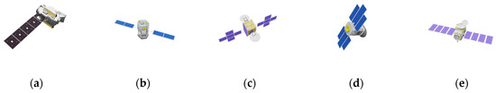
Figure 14. Partial display images of other satellites within the dataset. (a) IceSat; (b) OCO–2; (c) Galaxy–19; (d) CloudSat; (e) Jason–2.

This dataset will significantly support research in space object pose estimation, and 3D reconstruction. Concurrently, in terms of rendering speed, the imaging simulation method that integrates the improved Phong model and HOSH for space objects has achieved real-time fast imaging capabilities. The RSSF speed is approximately 2.86 s per frame, while the speed for SSPT is about 1.67 s per frame, which can sufficiently meet engineering demands to some extent.

6. Conclusions

In order to address the critical issue of image scarcity encountered by space-based optical cameras, this study introduces a method for optical imaging computation of space objects that integrates the improved Phong model and HOSH. It outlines a comprehensive research approach to the geometric and radiative rendering pipeline and clarifies the optical image data simulation process for spacecraft. Based on experimental measurements, this study derives material properties and lighting conditions, extracting variables such as metallicity, roughness, IOR, and Alpha. The improved Phong model not only enhances the capability of describing the Fresnel reflection phenomenon, but also strengthens its ability to characterize the scattering properties near the specular reflection direction. This research achieves a closed loop in the space-based optical imaging chain, producing datasets that contain imaging effects at various relative distances, accompanied by a corresponding 6D pose label.

References

- Zhu, W.S.; Mu, J.J.; Li, S.; Han, F. Research progress on spacecraft pose estimation based on deep learning. J. Astronaut. 2023, 44, 1633–1644. [Google Scholar]
- Sun, C.M.; Yuan, Y.; Lv, Q.B. Modeling and verification of space-based optical scattering characteristics of space objects. Acta Opt. Sin. 2019, 39, 1129001. [Google Scholar] [CrossRef]
- Peng, X.D.; Liu, B.; Meng, X.; Xie, W.M. Imaging simulation modeling of space-borne visible light camera. Acta Photon. Sin. 2011, 40, 1106–1111. [Google Scholar]
- Hu, J. Research on Imaging Effect Simulation of Space Camera Based on Monte Carlo Ray Tracing. Ph.D. Thesis, University of Chinese Academy of Sciences, Beijing, China, 2013. [Google Scholar]
- Huang, J.M.; Liu, L.J.; Wang, Y.; Wei, X.Q. Research on space target imaging simulation based on target visible light scattering characteristics. Aerosp. Shanghai 2015, 32, 39–43. [Google Scholar]
- Han, Y.; Chen, M.; Sun, H.Y.; Zhang, Y. Imaging simulation method of Tiangong-2 companion satellite visible light camera. Infrared Laser Eng. 2017, 46, 258–264. [Google Scholar]
- Xu, X.X. Imaging Simulation of Space-Borne Visible Light Camera for Space Targets. Ph.D. Thesis, University of Chinese Academy of Sciences, Beijing, China, 2020. [Google Scholar]
- Yang, J.S.; Li, T.J. Research on imaging simulation of space-based space target scene. Laser Optoelectron. Prog. 2022, 59, 253–260. [Google Scholar]
- Hong, J.; Hnatyshyn, R.; Santos, E.A.D.; Maciejewski, R.; Isenberg, T. A survey of designs for combined 2D+3D visual representations. IEEE Trans. Vis. Comput. Graph. 2024, 30, 2888–2902. [Google Scholar] [CrossRef]
- Musallam, M.A.; Gaudilliere, V.; Ghorbel, E.; Al Ismaeil, K.; Perez, M.D.; Poucet, M. Spacecraft recognition leveraging knowledge of space environment: Simulator, dataset, competition design and analysis. In Proceedings of the 2021 IEEE International Conference on Image Processing Challenges (ICIPC), Anchorage, AK, USA, 19–22 September 2021; pp. 11–15. [Google Scholar]
- Al Homssi, B.; Al-Hourani, A.; Wang, K.; Conder, P.; Kandeepan, S.; Choi, J. Next generation mega satellite networks for access equality: Opportunities, challenges, and performance. IEEE Commun. Mag. 2022, 60, 18–24. [Google Scholar] [CrossRef]
- Hu, Y.L.; Speierer, S.; Jakob, W.; Fua, P.; Salzmann, M. Wide-depth-range 6D object pose estimation in space. In Proceedings of the 2021 IEEE/CVF Conference on Computer Vision and Pattern Recognition (CVPR), Nashville, TN, USA, 19–25 June 2021. [Google Scholar]
- Price, A.; Yoshida, K. A monocular pose estimation case study: The Hayabusa2 Minerva-II2 deployment. In Proceedings of the 2021 IEEE/CVF Conference on Computer Vision and Pattern Recognition Workshops (CVPRW), Nashville, TN, USA, 19–25 June 2021; pp. 1992–2001. [Google Scholar]
- Cao, Y.; Mu, J.Z.; Cheng, X.H.; Liu, F.Y. Spacecraft-DS: A spacecraft dataset for key components detection and segmentation via hardware-in-the-loop capture. IEEE Sens. J. 2024, 24, 5347–5358. [Google Scholar] [CrossRef]
- Park, T.H.; D’Amico, S. Adaptive neural network-based unscented Kalman filter for robust pose tracking of noncooperative spacecraft. J. Guid. Control Dyn. 2023, 46, 1671–1688. [Google Scholar] [CrossRef]
- Li, T.J. Research on Monitoring Method and Imaging System Simulation of Space-Based Target Visible Light Camera. Ph.D. Thesis, Tianjin University, Tianjin, China, 2021. [Google Scholar]
- Yu, K. Research on Key Technologies of Space Target Photoelectric Detection Scene Simulation and Visual Navigation. Ph.D. Thesis, Harbin Institute of Technology, Harbin, China, 2020. [Google Scholar]
- Alexa, M. Super-Fibonacci spirals: Fast, low-discrepancy sampling of SO(3). In Proceedings of the 2022 IEEE/CVF Conference on Computer Vision and Pattern Recognition (CVPR), New Orleans, LA, USA, 18–24 June 2022; pp. 8281–8290. [Google Scholar]
- Bechini, M.; Lavagna, M.; Longhi, P. Dataset generation and validation for spacecraft pose estimation via monocular images processing. Acta Astronaut. 2023, 204, 358–369. [Google Scholar] [CrossRef]
- Ji, X.; Zhan, F.; Lu, S.; Huang, S.-S.; Huang, H. MixLight: Borrowing the best of both spherical harmonics and Gaussian models. arXiv 2024, arXiv:2404.12768. [Google Scholar] [CrossRef]
- Price, M.A.; McEwen, J.D. Differentiable and accelerated spherical harmonic and Wigner transforms. J. Comput. Phys. 2024, 510, 113109. [Google Scholar] [CrossRef]
- Li, P.; Li, Z.; Xu, C.; Fang, Y. Research on scattering spectrum of third-order gallium arsenide battery based on thin-film interference theory. Spectrosc. Spectr. Anal. 2020, 40, 3092–3097. [Google Scholar]
- Synopsys.org. Optical Scattering Measurements & Equipment. Available online: https://www.keysight.com/us/en/products/software/optical-solutions-software.html (accessed on 21 March 2025).
- Cao, Y.; Cao, Y.; Wu, Z.; Yang, K. A calculation method for the hyperspectral imaging of targets utilizing a ray-tracing algorithm. Remote Sens. 2024, 16, 1779. [Google Scholar] [CrossRef]
- Liu, Y.; Dai, J.; Zhao, S.; Zhang, J.; Li, T.; Shang, W.; Zheng, Y. A bidirectional reflectance distribution function model of space targets in visible spectrum based on GA-BP network. Appl. Phys. 2020, 126, 114. [Google Scholar] [CrossRef]
- Li, Z.; Xu, C.; Huo, Y.; Fang, Y. Principles and Applications of Optical Characteristics of Space Targets; Tsinghua University Press: Beijing, China, 2025. [Google Scholar]
- Pharr, M.; Humphreys, G. Physically Based Rendering: From Theory to Implementation, 2nd ed.; Morgan Kaufmann, Elsevier: Burlington, MA, USA, 2010. [Google Scholar]
- Walter, B.; Marschner, S.R.; Li, H.; Torrance, K.E. Microfacet models for refraction through rough surfaces. In Proceedings of the 18th Eurographics Conference on Rendering Techniques (EGSR ’07), Grenoble, France, 25–27 June 2007; Eurographics Association: Goslar, Germany, 2007; pp. 223–231. [Google Scholar]
- Schlick, C. An inexpensive BRDF model for physically-based rendering. Comput. Graph. Forum 1994, 13, 233–246. [Google Scholar] [CrossRef]
- Karis, B. Real Shading in Unreal Engine 4; Beijing Institute of Technology Press: Beijing, China, 2013. [Google Scholar]
- Ning, Q.; Wang, H.; Yan, Z.; Liu, X.; Lu, Y. Space-based THz radar fly-around imaging simulation for space targets based on improved path tracing. Remote Sens. 2023, 15, 4010. [Google Scholar] [CrossRef]
- Hell, M.C.; Horvat, C. A method for constructing directional surface wave spectra from ICESat-2 altimetry. Cryosphere 2024, 18, 341–361. [Google Scholar] [CrossRef]
- Proença, P.F.; Gao, Y. Deep learning for spacecraft pose estimation from photorealistic rendering. In Proceedings of the 2020 IEEE International Conference on Robotics and Automation (ICRA), Paris, France, 31 May–31 August 2020; pp. 1234–1238. [Google Scholar]
Disclaimer/Publisher’s Note: The statements, opinions and data contained in all publications are solely those of the individual author(s) and contributor(s) and not of MDPI and/or the editor(s). MDPI and/or the editor(s) disclaim responsibility for any injury to people or property resulting from any ideas, methods, instructions or products referred to in the content. |
© 2025 by the authors. Licensee MDPI, Basel, Switzerland. This article is an open access article distributed under the terms and conditions of the Creative Commons Attribution (CC BY) license (https://creativecommons.org/licenses/by/4.0/).