Highlights
What are the main findings?
- We developed and trained ResNet101-SCSE-U-Net for semantic segmentation of 16 benthic reef classes, achieving 84% overall accuracy, and modifications to the model were able to handle the highly unbalanced training data.
- The trained model was successfully applied to 27 unlabeled plots from 2023, demonstrating strong generalizability and providing a tool for automated monitoring of new reef surveys.
What are the implications of the main findings?
- We provide a reproducible, step-by-step pipeline for fully supervised deep learning-based annotation of coral reef imagery, reducing the reliance on manual labeling by experts.
- The pipeline and trained models can be transferred across reef environments, capturing ecological variation and enabling fully automated, high-resolution classification of benthic communities.
Abstract
Habitat complexity plays a critical role in coral reef ecosystems by enhancing habitat availability, increasing ecological resilience, and offering coastal protection. Structure-from-motion (SfM) photogrammetry has become a standard approach for quantifying habitat complexity in reef monitoring programs. However, a major bottleneck remains in the two-dimensional (2D) classification of benthic cover in three-dimensional (3D) models, where experts are required to manually annotate individual colonies and identify coral species or taxonomic groups. With recent advances in deep learning and computer vision, automated classification of benthic habitats is possible. While some semi-automated tools exist, they are often limited in scope or do not provide semantic segmentation. In this investigation, we trained a convolutional neural network with the ResNet101 architecture on three years (2015, 2017, and 2019) of human-annotated 2D orthomosaics from Kiritimati, Kiribati. Our model accuracy ranged from 71% to 95%, with an overall accuracy of 84% and a mean intersection of union of 0.82, despite highly imbalanced training data, and it demonstrated successful generalizability when applied to new, untrained 2023 plots. Successful automation depends on training data that captures local ecological variation. As coral monitoring efforts move toward standardized workflows, locally developed models will be key to achieving fully automated, high-resolution classification of benthic communities across diverse reef environments.
1. Introduction
Habitat complexity plays a vital role in ecosystem function and diversity, offering numerous benefits, including enhanced habitat provisioning, increased resilience, and effective coastal protection [1,2,3,4]. Complex and dynamic habitats promote resilience by providing greater niche availability and refugia across multiple spatial scales [5,6,7,8,9]. Increased habitat complexity is positively associated with species richness, abundance, and diversity across most benthic ecosystems [1]. For example, fish abundance in coral reefs has been closely linked to structural complexity [10,11,12,13,14].
To quantify reef complexity, many monitoring programs now incorporate outputs such as rugosity, curvature, and vertical relief derived from photogrammetric surveys. However, while the physical complexity of reefs can be semi-automatically processed using tools like digital surface models (DSM) and orthomosaics, the classification of benthic communities still depends heavily on manual expert annotation. This reliance on expert input is both time consuming and resource intensive, contributing to persistent undersampling of benthic communities [15,16,17,18]. Recent advances in computer vision and machine learning, specifically semantic segmentation using neural networks, offer a promising path forward by automating benthic classification and helping bridge the gap between data collection and ecological interpretation [19,20].
Semantic segmentation, which assigns a class to every pixel in an image, is a widely used method in image analysis [21]. While other techniques are also used, such as random point identification, object detection, and instance segmentation, semantic segmentation may be a more suitable option for marine applications owing to the complexity of underwater environments and their organisms. In this context, automation refers to the use of algorithms to perform tasks, such as identifying and classifying benthic features, that would otherwise require manual annotation. It has been applied in various contexts, including invertebrate detection in Antarctica, mapping sponge behaviors, and assisting with megafauna species identification and population counts [22,23,24,25,26].
One of the earliest applications of neural networks for benthic classification was CoralNet, a tool that remains widely used [27]. CoralNet facilitates the semi-automated annotation of benthic imagery, using human-identified random point classifications to estimate the percentage composition of each class [27,28]. While CoralNet has a strong training dataset for point-based analysis, it lacks image segmentation capabilities and cannot integrate higher dimensional data such as DSMs or orthomosaics. TagLab was the first semi-automated program designed for orthomosaic imagery and 3D models, combining interactive, pixel-wise segmentation with an automated learning pipeline to develop robust semantic segmentation models for benthic mapping [29]. More recently, there has been an increase in the diversity of neural networks for benthic classification. Hopkinsons et al. [30] integrated 3D models with imagery acquired via SfM photogrammetry, leveraging the combined dimensionality to improve classification outcomes. Other recent tools, like DeepReefMap, focus on speed and versatility, enabling the automated classification of video data collected by drones and autonomous underwater vehicles (AUVs). While these systems provide practical solutions for large-scale surveys, they typically achieve moderate classification accuracy, ranging from 60% to 85%, and coarse benthic classes, such as coral, algae, substrate, and sand [31]. By contrast, an imaging spectroscopy (hyperspectral) approach that combines spectroscopy with 3D models offers finer taxonomic resolution and reported accuracies of 90–96%. However, this method requires highly specialized equipment called the HyperDiver [18], greatly limiting its availability.
Even more recently, the exponential rate of advancements in computer vision and machine learning has led to an increase in automated approaches for benthic habitat classification, particularly through the use of convolutional neural networks (CNNs) and semantic segmentation techniques. Semantic segmentation has emerged as the dominant method due to its ability to capture fine-scale spatial heterogeneity in complex environments like coral reefs. Several recent studies have demonstrated the applicability of CNN-based approaches in this context, including those that leverage point annotations [29,30], pretrained general-purpose models [32], or voxel-based architectures [33]. These studies often rely on relatively small training datasets (typically 3–8 plots), point-based annotations, minimal to no applications on new datasets, or limited temporal coverage, which can constrain the ecological generalizability of models. For example, Remmers et al. [32] introduced the RapidBenthos pipeline, which combines a pre-trained segmentation model (SAM) with multi-viewpoint annotations to classify reef imagery with minimal manual effort. While highly efficient and capable of classifying over 40 taxa within individual plots, the method relies on sparse point labels from ReefCloud, limiting its ability to generalize to fully labeled datasets or across time. It also cannot measure growth or mortality, nor fully capitalize on the fine spatial resolution of data. Therefore, there is a trade-off between taxonomic resolution and ecological metrics, where point-based classification offers higher taxonomic specificity while pixel-level segmentation enables the measurement of ecological processes such as growth and mortality and temporal changes. One group presented a middle ground approach by combining sparse point-based annotations with superpixel-based delineations, enabling improved semantic segmentation performance while reducing labeling effort [34,35].
Despite the recent increase in the number of studies attempting to automate the classification process, many coral monitoring programs still heavily rely upon manual digitization for benthic classification [28]. This process is labor intensive, time consuming, and costly, yet it has generated an extensive repository of annotated vector layers with high-resolution 3D models and 2D orthomosaics. These datasets remain underutilized for the development of automated classification systems, representing a valuable resource for training next-generation neural network models.
Here, we developed a CNN containing the U-Net architecture [36] with a ResNet101 encoder and a Spatial and Channel Squeeze & Excitation (SCSE) block, specifically designed to automate the digitization of coral reef communities from 2D Red, Green, Blue (RGB) orthomosaic photos. The model was trained using complete pixel-level annotations across 77 plots surveyed in 2015, 2017, and 2019. We had between 16 and 27 benthic classes and one background, including living coral morphologies, macroalgae, and non-living substrate types. We then ran the fully trained model on 28 unlabeled sites from 2023. We included significantly more classes than most comparable pixel-based annotation studies and had one of the most temporally resolved datasets for automated benthic classification [31,34,35]. Our objective was not only to improve classification accuracy but to provide open-source, user-friendly code that is easy to implement and adaptable to local reef contexts. Given the complexity and variability of coral reef ecosystems, scalable automation depends on diverse and well-labeled training data. As the field continues toward standardization, developing locally trained models remains essential for building robust and transferable pipelines for benthic community classification.
2. Methods
2.1. Data Acquisition: Study Site, Plots, and Mega Photo Quadrats
To quantify the change in reef complexity, annual expeditions to Kiritimati (Christmas Island), Republic of Kiribati, were conducted before the onset of (May 2015) and following the mass coral bleaching event caused by the 2015–2016 El Niño-induced marine heat wave, which resulted in 89% mortality of all living hard coral around the island [37]. Thirty permanent 4 × 4 m plots (labeled as mega photo quadrats (MPQs)) were marked with rebar for relocation and resurveyed annually. These MPQs were established using structure-from-motion (SfM) photogrammetry techniques at 10 shallow forereef sites (3 MPQs per site) on Kiritimati (Christmas Island; Republic of Kiribati) and were revisited in subsequent years to monitor temporal changes within the same spatial footprint (Figure 1). The 10 sites were categorized into three levels of human disturbance gradients: low, medium, and high (as detailed in [17,37]). At each site, the three permanent MPQs were approximately 10 m apart along a 10 m to 12 m isobath. The MPQs were surveyed annually from 2015 to 2023, except for the period from 2020 to 2022 due to COVID-19 travel restrictions. Data from 2015, 2017, 2019, and 2023 were used for this investigation. Some sites could not be surveyed in certain years due to accessibility issues; for example, sites 15 and 19 were not surveyed in 2019 because of south swells generated by three consecutive hurricanes over the Hawaiian Islands. A full description of the sites is available in [38].
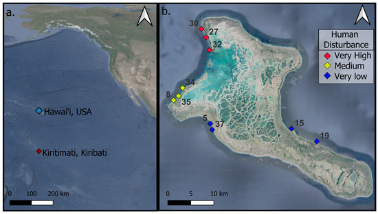
Figure 1.
Map of Kiritimati, Kiribati, showing (a) its location in the Pacific Ocean and (b) a detailed island map with site locations.
2.2. Data Preprocessing: 3D Models, Benthic Community Digitization, and Data Conversion
Images were collected using SfM photogrammetry techniques described in [15], and a detailed description of these field methods from Kiritimati is provided in [17]. Between 400 and 800 images were collected for each MPQ (plot). Ground control points and scale bars were placed at the corners of the MPQs (plots) for scaling and orthorectification. A diver collected overlapping (70–80%) planar images while swimming roughly 1 m to 2 m above the benthos in a boustrophedonic or lawn-mower pattern. Images were captured using a Nikon D750 DSLR with a 24 mm Sigma lens, housed in an Ikelite underwater system with an 8-inch hemispheric dome port. The images were automatically processed using Agisoft PhotoScan software 2.2.1 [39] to produce 3D models with a resolution of <0.01 cm and then scaled up to a resolution of 1 cm. The outputs included a DSM, an orthomosaic photo, a 3D mesh, and a 3D point cloud for each plot. We manually annotated the benthic surface composition on each 2D orthomosaic using the digitization tool in ArcMap 10.8.2 [40] to create a benthic cover map for each plot in 2015, 2017, and 2019. The benthic cover map categorized the substrate into 27 morphological classes and one background class in the orthomosaics with NaN values (labeled class 127; Table S1). A trained technician used the digitization tool in ArcMap to manually delineate polygons around living coral colonies, dead coral, and inorganic substrate, assigning each polygon to 1 of the 27 predetermined morphology classes (Table S1). Digitizing each plot required 6 to 10 h of labor, with more time needed for plots with high live coral cover. The final output for each plot was a multi-polygon shapefile that delineated benthic cover, including individual coral colonies.
In total, we processed 77 plots (one orthomosaic per plot) from 2015, 2017, and 2019 and 27 from 2023 (Table S2). Using ArcMap, we clipped and trimmed the orthomosaics and benthic cover polygons to ensure consistent extents for each plot. In ArcMap, the classified polygons were then rasterized and converted into a mask (classes were assigned a number instead of a category; Table S1) to be used as labels for the training data. The mask rasters were generated at the same resolution and with the same pixel dimensions as the orthomosaics, ensuring that each pixel was assigned either a benthic class or the background class. Since the orthomosaics were very large (>10,000 by 10,000 pixels), we divided each image and mask into tiles of 512 by 512 pixels. Tiles at the right and bottom border were padded and labeled as background class 127. The masks were converted into a one-hot encoded vector, which was essential for transforming categorical data into a format suitable for multi-class semantic segmentation. Examples of tiles are shown in Figure S1, and a simplified example of this process is illustrated in Figure 2. For the CNN training, only 2D orthomosaics were used; we did not include the 3D outputs from the SfM pipeline to increase the potential for transferability of the model.
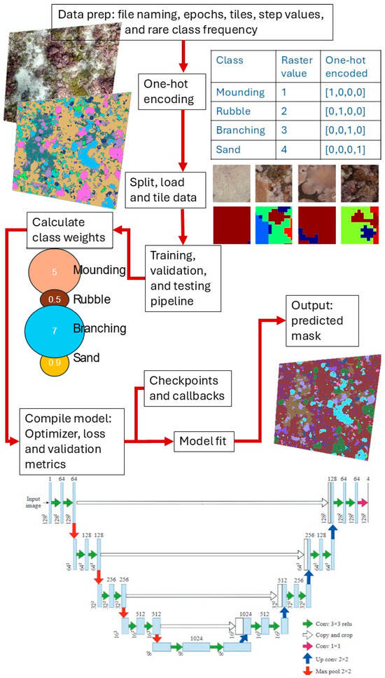
Figure 2.
Flowchart depicting the key stages of the convolutional neural network classifier, including data preprocessing, model training, classification, and post-processing steps. The original U-Net architecture diagram was published in [36].
2.3. Data Processing: Training Pipeline, U-Net Modifications, and Building the Model
The CNN model was trained on 125,901 tiles from the subsetted orthomosaics (plots) and masks from 2015, 2017 and 2019, and it was subsequently applied to predict masks that aligned with the orthomosaics (plots) from 2023 (Table S2). While the architecture of the CNN model followed a standard U-Net framework [26,36], we made several modifications to improve training stability, efficiency, and performance. To enhance generalizability and address uneven class distributions, we incorporated data augmentation, class weighting, and tile boosting of rare classes. We reduced overfitting through regularization techniques. These adjustments stabilized training, decreased processing time, and improved the ability of the model to handle the uneven class distribution.
2.3.1. Training, Validation, and Testing Pipeline
A training, validation, and testing pipeline was developed to ensure efficient data loading and transformation, thereby improving model generalizability and performance. Training, validation, and testing were randomly split across all of the compiled tiles: 70%, 15% and, 15%, respectively. We pooled all 125,901 tiles, partitioned them into training, validation, and test sets using spatially disjoint splits along the x-axis and y-axis to minimize spatial autocorrelation and ensure non-overlapping regions across splits [41]. The training/validation/testing pipeline included data preparation and prefetching (loading the next set of data while the current batch is processing) using ‘autotune’ from TensorFlow, one-hot encoding of NumPy mask files, storage as TensorFlow record files [42,43], and concurrent parallel loading of image tiles with optimized batching [42,44]. To further improve generalizability, data augmentation and shuffling were integrated. Data augmentation applied random transformations such as rotation and flipping. These techniques increased dataset diversity, enabling the model to better adapt to unseen data. By combining random augmentations with shuffling, the pipeline also mitigated overfitting and improved performance, particularly for underrepresented classes. The validation and testing pipelines followed the same structural framework as the training pipeline but excluded augmentation and shuffling to conserve computational resources. The testing portion of the pipeline was only used for final model evaluation and predictive performance. All datasets were cached to local scratch storage to further reduce latency and ensure reproducibility across training runs.
2.3.2. CNN Model Architecture Implementation
We implemented the U-Net architecture using TensorFlow and Keras API with a ResNet101 encoder and Spatial and Channel Squeeze and Excitation (SCSE) attention blocks decoder [36,42,45]. The ResNet101 backbone, pretrained on ImageNet, was used as the encoder (contracting path), where residual blocks enabled deep feature extraction and mitigated vanishing gradients via identity skip connections [45]. The decoder (upsampling path) comprised transposed convolutional blocks concatenated with corresponding encoder features. Each decoder stage included a convolutional layer, max pooling, batch normalization, ReLu activation, and an SCSE block to recalibrate features spatially and channel-wise. SCSE blocks combine channel-wise attention via global average pooling (cSE) with spatial attention (sSE), enhancing the focus of the model focus on semantically important regions [45,46,47]. SpatialDropout2D was applied after each decoder block to reduce overfitting. A final 1 × 1 convolution with softmax activation produced class probabilities and predictions for multi-class semantic segmentation [48]. We used softmax activation because we had a multi-class classification in our semantic segmentation [48]. A full list of the hyperparameters can be found in Table 1, with descriptions provided in Section 2.5.

Table 1.
Hyperparameters for model architecture, training settings, and data handling for the ResNet101-based segmentation model.
To address class imbalance in the training data, we calculated pixel-level class frequencies across all training masks prior to tiling. Rare classes were identified as those with a frequency below half the median class frequency. During tiling, we duplicated tiles containing at least one rare class by a factor inversely proportional to the frequency of that class. Specifically, the duplication factor was calculated as the ratio of the median class frequency to the frequency of the rarest class present in the tile, capped between 1 and 10 to prevent overrepresentation. This targeted oversampling strategy ensured that rare but important benthic classes contributed more meaningfully during model training. To further mitigate the class imbalance, we used a combined loss function of focal and Dice losses with integrated class weights and label smoothing [49,50]. Class weights were calculated using the inverse log-frequency of class occurrences across all training data and normalized to 1.0. Weights were used to scale the focal loss to reduce bias toward the dominant classes. Dice loss was computed per image and weighted more heavily to ensure shape and boundary alignment were maintained. A label smoothing factor of 0.1 was applied to soften hard class assignments and improve generalizability [51].
All masks were one-hot encoded (Figure 2). We used an AdamW optimizer (weight decay of 1 × 10⁻⁵) with gradient clipping to stabilize training and prevent exploding gradients (hyperparameters can be found in Table 1; [52,53]). The model was compiled using a combined focal and Dice loss, with accuracy and the Dice coefficient evaluated as performance metrics. The model fitting process involved defining the training and validation datasets, specifying the number of epochs, setting the steps per epoch and validation frequency, applying class weights, and integrating monitoring callbacks (Table 1). This was the most time-consuming and computationally expensive phase, as it determined the overall model performance. The model was trained for the full 50 epochs. Each mask output was reassembled into a raster.
We conducted multiple rounds of convolutional neural network (CNN) model development using high-performance computing clusters and cloud services offered through the Digital Research Alliance of Canada. On these high-performance cluster servers, we used 250 GB of RAM and 1 NVIDIA A100S × M4 GPU with 40 GB of memory.
2.4. Data Post-Processing: Validation, Overfitting, and Model Comparison
Model performance was assessed on the testing data across all 27 benthic classes and one background class using accuracy metrics, including overall accuracy, the Dice coefficient, and loss. The model was then applied to predict new masks for data from 2015 to 2019. Only 16 classes were meaningfully predicted, and these were used to evaluate pixel- and class-level performance, including precision, recall, F1 score, and mean intersection over union (mIoU), to assess mask accuracy. The performance of the CNN was evaluated using a combination of metrics to ensure its accuracy, robustness, and generalizability. Learning curves for training and validation loss, as well as accuracy, were analyzed over epochs to assess model convergence, underfitting, and overfitting. To evaluate classification performance, we used a confusion matrix to compare the ground truth classes with the predicted classes. Only classes that were predicted correctly at least once were included in the matrix, resulting in 16 out of the 27 original classes. The confusion matrix was row-normalized to show, for each ground truth class, the percentage of pixels predicted as each class. We calculated per-class and per-site performance metrics, including intersection over union (IoU), precision, F1 score, and recall.
To evaluate model performance, we benchmarked SCSE U-Net with the ResNet101 backbone architecture against three commonly used CNN baselines: a standard U-Net, a fully convolutional neural network (FCNN), and a DenseNet-based model [36,54,55]. Performance was assessed using four metrics: test accuracy, the Dice coefficient, loss, and mean intersection over union (mIoU).
2.5. Applications to New Data
The trained model was applied to the unlabeled 2023 orthomosaics to evaluate its performance on imagery not included in the training or validation sets. Predicted masks were generated for each plot, and to provide a basis for assessment, we also prepared a small number of independent example masks that were manually annotated but not used in model development. These example masks allowed for direct visual comparison with the model outputs, confirming that the predicted classes aligned with the expected cover types, such as living coral types, rubble fields, and sand areas. This procedure provided additional validation of model generalization and demonstrated its utility for generating classifications in datasets that lack complete manual annotation.
3. Results
3.1. Model Performance
We provide a workflow that outlines the main processing steps in Figure 2. We introduced key modifications to the standard U-Net architecture and other CNN components to ensure that the model was well suited for our large, multi-class, multi-year, and spatially variable dataset. Some of these changes included ensuring that segmentation masks were properly one-hot encoded, implementing effective data augmentation strategies to increase dataset variability, calculating class weights, and selecting an appropriate optimizer and loss function (Table 1). These modifications significantly improved the ability of the model to learn global patterns, generalize new data, and converge efficiently during training.
To evaluate model training and validation while running the model, we tracked accuracy, loss, and Dice coefficient curves and the learning rate, all of which showed a good fit. The training and validation values remained closely aligned throughout all 50 epochs, and the learning rate decreased steadily during training (Figure 3). The steady increase and agreement in training and validation accuracy scores and Dice coefficients, along with the steady decrease in losses, indicated that the model effectively captured key features of the input data, supporting its ability to generalize and make accurate predictions (Figure 3; Table 2). We added a mixed-precision in-memory training function (faster training by using mixed datatypes), which almost doubled the training speed but introduced substantial instability and exploded gradients.
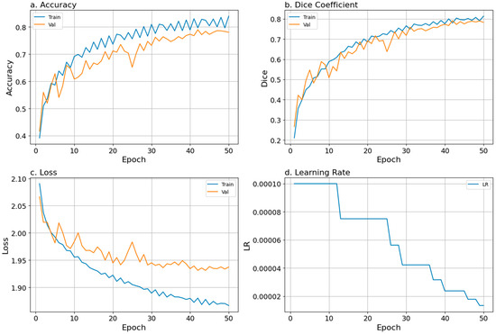
Figure 3.
Training performance over 50 training epochs is shown as (a) accuracy, (b) Dice coefficient, (c) loss, and (d) learning rate. Blue and orange lines represent smoothed epoch means for training and validation metrics, respectively. The blue line in panel (d) shows the scheduled learning rate used during training.
Table 2.
Model performance metrics (loss, Dice coefficient, accuracy, mean IoU) across training, validation, and testing datasets.
SCSE U-Net with the ResNet101 backbone showed strong training, validation, and testing performance, with Dice coefficients of 0.81, 0.78, and 0.64, and corresponding losses of 1.87, 1.94, and 2.34, respectively (Table 2). These metrics indicated good pixel-level generalizability, even on held-out test data. Class-level metrics, namely mIoU, precision, F1 score, and recall, were stronger than the pixel-level metrics at both the class and site levels (Tables S3 and S4). The overall mIoU was 0.82, reflecting strong model performance, particularly given the heavily imbalanced dataset (Table S3). Most class-level IoU scores were high, ranging from 0.71 to 0.92, with the exceptions of Live Massive Grooved (0.52), Soft Coral Nodular (0.03), and Dead Foliose (0.46), which were impacted by mislabeling in one or two plots (Table S3). At the site level, both mIoU and accuracy remained strong, with mIoU scores ranging from 0.70 to 0.80 and accuracy scores ranging from 0.83 to 0.95 (Table S4). One exception was Site 32, with an mIoU of 0.52 and an accuracy of 0.85, which was mostly Rubble and Dead Massive.
3.2. Model Outputs and Application to New Data
In general, plots with more living coral produced more accurate masks, potentially because the Dead Massive and Rubble classes exhibited greater internal variability, often including cover by crustose coralline algae, sand, or microalgae. Despite these challenges, the predicted masks remained robust, capturing key spatial patterns across most sites. For example, in Site 5, Plot 1 (Figure 4), where data were taken four years apart, the model captured ecological change following the 2015–2016 El Niño event. Coral cover and benthic diversity declined sharply, which showed an increase in the dead massive coral class in 2019. One error occurred in Site 5 MPQ1, where we observed a large Non-Coral Submassive cover on the far left of the true mask, but it was predicted as Non-Coral Submassive (Figure 4a,b).
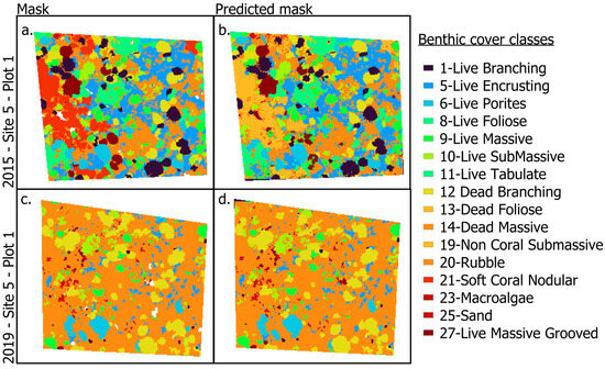
Figure 4.
Examples of inputs and outputs used in the CNN classifier ground truth masks (a,c), and the resulting predicted classification masks (b,d) for Site 5, Plot 1, in 2015 and 2019, highlighting the progression from image acquisition to automated classification.
The confusion matrix showed classification accuracy and misclassification patterns based on the 2015, 2017, and 2019 datasets (Figure 5 and Figure S3). Only 16 of the 27 benthic cover classes were consistently predicted (background class 127 was excluded), which matched the class distribution of the true masks. The best-predicted classes were primarily living coral types, except for Live Massive Grooved, which was often confused with Live SubMassive, and Foliose for Live Branching, because of similarities in morphology and color (Figure 5). Small coral colonies were also a challenge, likely due to their limited spatial extent and underrepresentation in the training dataset. In the non-living classes, Dead Massive, Rubble, and Dead Branching all had the highest accuracy (Figure 5). However, distinguishing between hard inorganic and dead substrates was more difficult than discerning living coral classes. These findings were consistent with the per-class performance metrics IoU, precision, and recall (Table S3).
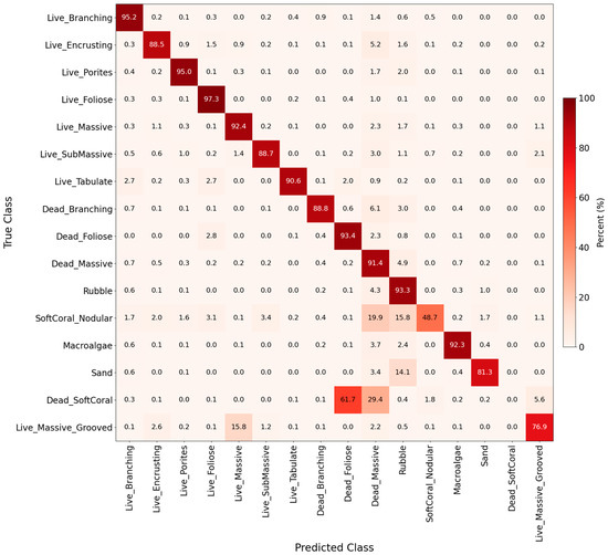
Figure 5.
Normalized confusion matrix as a heatmap, representing classification performance across 16 benthic classes (background class 127 was not included). Each cell indicates the percentage of pixels from a true class (rows) predicted as a given class (columns). Percentages are computed across all validation images from 2015–2019 combined.
We benchmarked the performance of three standard CNN architectures, U-Net, FCNN, and DenseNet, against our proposed ResNet101-SCSE-Unet model for benthic segmentation (Table 3). ResNet101-SCSE-Unet achieved the highest mIoU score of 0.83, significantly outperforming all other models, which each reached an mIoU of only 0.48. While DenseNet matched our model in overall test accuracy (0.64) and Dice coefficient (0.66), it fell short in class-level agreement, as reflected in its lower mIoU score. The U-Net and FCNN models demonstrated noticeably lower test accuracy scores (0.43 and 0.39, respectively) and Dice coefficients (0.34 and 0.27), with higher loss values than DenseNet and our model. These results demonstrated that ResNet101-SCSE-Unet offers substantially improved class-wise prediction accuracy and segmentation consistency compared to commonly used CNN baselines.
Table 3.
Test accuracy, Dice coefficient, loss, and mean intersection over union (mIoU) are reported for each convolutional neural network (CNN) architecture evaluated on the benthic segmentation task.
The predicted and observed class proportions were highly consistent across years, with the vast majority of differences falling within ±0.01, underscoring the ability of the model to predict benthic cover with high accuracy (Table S5). This indicated that the model effectively captured both dominant and rare classes across multiple time points. Notable exceptions included an overestimation of Dead_Foliose in 2017 (+0.035) and rubble in 2019 (+0.026), as well as underestimation of Dead_Tabulate and SoftCoral_Plating (Table S5). Several live coral categories, such as Branching, Foliose, and Massive morphologies, were modestly overpredicted in 2015 but showed much smaller discrepancies by 2019, reflecting improved generalization over time. Despite small localized biases, the overall magnitude and direction of prediction errors were small or even negligible, and comparable to human error.
We evaluated generalization on 2023 plots with ground-truth masks held out from training (Site 8, Plot 2; Site 34, Plot 1; and Site 35, Plot 1; Figure 6). Despite minor tiling artifacts visible in some scenes, predictions closely matched the withheld annotations and, in several instances, delineated coral colonies that were absent from the human-labeled plots. Predicted boundaries were contiguous and smooth, reducing stair-step effects common in manual labels. Qualitative inspection indicated that the model captures fine-scale morphological detail and within-plot heterogeneity that can be difficult to annotate consistently, supporting its use for mapping in years lacking annotations.
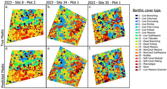
Figure 6.
Hold-out examples from 2023 data. True masks (not used for training) and corresponding predicted masks for three plots: (a,b) Site 8, Plot 2; (c,d) Site 34, Plot 1; (e,f) Site 35, Plot 1. In each pair, the left panel shows the true masks, and the right panel shows the model prediction on 2023 imagery not seen during training. The colors differ slightly from those used for benthic types in Figure 4.
4. Discussion
4.1. Automation of Annotated Coral Reef 3D Modeling
Here, we provide a step-by-step guide on automating the annotation of coral reef imagery using a fully supervised deep learning model. In contrast to traditional manual annotation, which is time consuming, labor intensive, and often inconsistent, our approach enables scalable, repeatable classification of complex benthic features at the pixel level. Our ResNet101-SCSE U-Net model achieved a strong mIoU of 0.83, demonstrating high classification accuracy across diverse reef habitats around Kiritimati and across a temporally resolved dataset. Our model proved to be effective for large-scale benthic monitoring. Moreover, the strong agreement between true and predicted masks gives us confidence in the accuracy of predictions on previously unlabeled 2023 data. When compared with benchmark CNN architectures, our model consistently outperformed others at both the pixel and class levels, highlighting its ability to handle a highly imbalanced dataset.
By automating classification across high-resolution 2D reef reconstructions, our approach addresses a major bottleneck in coral reef monitoring: the need to process large volumes of photogrammetric data with consistency and speed. This is particularly critical for repeat surveys aiming to detect ecological change over time. In reducing dependence on manual annotation, our framework increases scalability and reproducibility. We applied multiple checks and safeguards so that the data were not overfit. Our workflow offers a clear breakdown of the process, along with recommendations for modifying the code (Figure 2). For further details, readers can refer to our Zenodo v1 public archive, where we provide additional resources to help researchers apply this method to their own datasets.
4.2. Comparison with Recent Literature
Most recent studies on benthic classification rely on limited datasets, typically using only 3 to 8 plots, collected at a single time point, and trained on point annotations rather than full pixel-level labels. These models often include only a few or broad benthic classes and are rarely applied to new unlabeled data [30,31,32,56,57]. By contrast, our approach is built on a densely pixel-level annotated and available benthic dataset, comprising 77 fully labeled plots across five years (three time points 2015, 2017, and 2019), with dense pixel-level annotations across 27 benthic classes, later reduced to 16 after training.
Some more recent studies have developed innovative workarounds to overcome sparse annotations, for example, by using superpixels to propagate point labels, reporting improvements of 5–10% mIoU compared to other point-sampled methods [34]. Others have addressed specific technical challenges within the semantic segmentation pipeline: the authors in [58] applied dense labeling to video object segmentation; those in [59] benchmarked architectures for pixel-wise segmentation of two target species; and those in [60] combined improved color correction with colony-level classification and pixel-level labeling. While these studies contribute valuable technical advancements, they remain limited either in ecological scope, taxonomic breadth, or temporal resolution. Our study explicitly incorporates temporal dynamics by training models on multi-year data and applying them to 27 unannotated plots from 2023. Our dataset captures both spatial and temporal ecological gradients, supporting the development of models with greater generalizability and ecological relevance.
In parallel with technical advances, there has been a rise in the number of publications proposing automated classification pipelines for SfM-derived reef imagery. However, few offer a comprehensive, user-friendly workflow like the one presented here. Some recent studies eliminate the need for local training data by leveraging pre-trained models from large citizen science programs, while others focus on imagery from drones or UAVs [32,57]. Despite these innovations, manual annotation remains a key bottleneck for many organizations using SfM photogrammetry in routine monitoring [61]. Our workflow directly addresses this gap, as it is particularly well suited for research groups already generating human-labeled data, allowing them to train their models and automate future analyses. This could also be a limitation, as most coral annotations are made at the point level, while generating pixel-level labels for training is time consuming and labor intensive. While we designed our method with a specific audience in mind, it is adaptable, and we have provided sufficient technical details to make the pipeline accessible to non-specialists. Beyond benthic classification, this approach contributes to the broader effort to bridge the gap between quantitative computer vision methods and applied ecological research.
4.3. Model Improvements, Limitations, and Benchmark Comparisons
One of the most significant improvements we made was addressing the severe class imbalance. Unlike studies using fewer plots or coarser class groupings, our dataset had more variation across space and time. To improve the performance of predicting rare classes, we used rare class boosting during preprocessing by duplicating tiles containing underrepresented classes. We also applied data augmentation and used log-scaled class weights in a combined focal and Dice loss, helping the model to learn from both rare and dominant classes more effectively.
To prevent overfitting and improve generalizability, we added several regularization techniques, including spatial dropout (which disables random neurons during training) and weight decay (which penalizes large weights; Table 1). We tested multiple backbone architectures, namely ResNet50, ResNet152, and ResNet-101, and selected ResNet-101, which balanced depth and computational efficiency [45]. We also used early stopping and learning rate scheduling during training. Specifically, we monitored validation accuracy and loss, stopping training if no improvements were seen. The ReduceLROnPlateau callback lowered the learning rate when progress stalled [62]. These strategies prevented overfitting and resulted in stable convergence. Together, these adjustments, focused on class balancing, efficient data handling, and regularization, significantly improved training speed, model stability, and performance across all classes.
During training, we included all 27 classes and one background, but despite increasing the representation of rare categories, we reduced this to 16 classes to assess changes over time in benthic classes (Tables S1 and S3). We did not retrain the model on the 16 valid classes, which may have led to lower testing accuracy (0.64; Table 2). One challenge was inconsistent expert labeling, particularly in distinguishing rubble or other dead coral types from dead massive coral, which led to the overestimation of mortality and confusion during model training. When morphology was not distinguishable, it was classified as Rubble; otherwise, it was defaulted to Dead Massive or, to a lesser extent, Dead Branching when the colony morphology was still apparent. This may have led to an overestimation of Dead Massive and an underestimation of other dead classes. For example, Dead Soft Coral, Dead Columnar, Non-Coral Massive, and Non-Coral Branching were frequently misclassified as Dead Massive (Figure S3). All of the removed classes had an IoU of 0.0, which was due to their absence in the human annotations, such as three of the non-coral classes (branching, encrusting, and massive), or because they had too few examples (Table S3). Class-level IoU scores were generally high with a few exceptions, and sites with the highest coral cover performed best, suggesting that living coral taxa were much more distinct than dead or non-living substrates.
The three benchmark architectures performed worse than our model. Both U-Net only and FCNN showed low testing accuracy and mean IoU scores (0.43 and 0.39 for accuracy; 0.48 each for mean IoU; Table 3) [36,54]. This demonstrates their limited ability to capture the diversity and uneven distribution of benthic classes. Interestingly, DenseNet achieved the same testing accuracy as our model (0.64), which reflects pixel-level agreement. However, the mIoU scores differed significantly, where DenseNet had an mIoU of 0.48, compared to 0.82 for our model. As the mean IoU is calculated at the class level, this difference shows the ability of our model to outperform standard architectures and highlights the importance of modifying standard CNN models to the specific data characteristics, such as when dealing with highly imbalanced classes, as is common in benthic classification. DenseNet may have struggled with edge segmentation, leading to poor mask boundary overlap and explaining the discrepancy between its pixel accuracy and class-level performance (mIoU). By contrast, our model produced sharper, more confident predictions that better handled edges, resulting in improved overlap between predicted and true masks. This indicates that our model generalizes across classes, rather than only performing well at pixel-level accuracy.
4.4. Application to New Data and Ecological Implications
The temporal resolution of our dataset and the permanent nature of our plots allowed us to effectively classify 28 non-annotated plots from 2023. The differences between the predicted and true masks were negligible, giving us confidence in the accuracy of the newly predicted masks (Figure 6). Most recent studies in the emerging field of automated classification within the SfM pipeline do not include time series data or application to large unlabeled data. One notable exception is Coralscapes (currently a preprint), which shows promising results and strong performance on new, unlabeled data. Coralscapes captures 39 classes using semantic segmentation for generalizable performance with GoPro Hero 10 cameras. However, the timing of the surveys is not specified in the preprint, and the dataset does not appear to include any time series component.
Improving the performance of the model on new data may require additional manual annotations and training data that better reflect differences in data conditions, such as lighting, habitat types, or image quality. Annotating a small subset of new plots can help to assess model accuracy and guide decisions about broader application. Much like other machine learning algorithms, some local variability will always decrease the efficacy of the model when new data are introduced [63,64]. However, as models and machine learning algorithms improve, there may be simple adaptations to models such as this one. This model will be used in future expeditions for our group, and the level of detail left in this paper is meant to guide future colleagues but also inform other coral ecologists of the steps necessary to make benthic annotations faster.
Overall, the model predictions aligned well with ground-truth proportions for most benthic classes, with differences generally within ±0.01% across years (Figure S4; Table S5). This high level of accuracy indicates that the model was able to reliably reproduce community composition and capture the relative abundances of both dominant and rare groups. A small number of classes exhibited some minor divergence, reflecting systematic biases: Dead_Foliose was slightly overestimated in 2017, and rubble in 2019, while Dead_Tabulate and SoftCoral_Plating were consistently underestimated, likely due to their rarity and morphological similarity to other classes. Notably, predictions for major live coral groups (Branching, Foliose, Massive) were robust and converged closely with the observed values, demonstrating the ability of the model to generalize well across years and sites. Taken together, these results demonstrate that the model had strong predictive accuracy, with only a few systematic sources of error, reinforcing its suitability for quantitative assessments of benthic composition and its application in long-term monitoring frameworks.
Using the 2023 hold-out plots (not used in training), we found that the model works well on new data and adds value when labels are incomplete. Small tile artifacts are visible, but the predictions usually have smooth, continuous edges and, in several cases, outline colonies that human labeling missed (Figure 6). This shows that the model can pick up fine detail that is hard to capture by hand in crowded, mixed habitats. A practical use of the model is to let it pre-label new images and have experts review and correct the labels, rather than labeling everything from scratch. We should still guard against over-smoothing, which could merge small colonies or narrow gaps. Potential improvements could be to reduce tiling artifacts (more overlap with weighted blending, test-time augmentation) and sharpen edges (boundary-aware loss or post-processing). For measurement, we will pair mIoU with the boundary F-score, add colony-level detection/recall, and use uncertainty maps to flag low-confidence areas. Together, these steps support using the model to map years without labels while limiting false positives and smoothing errors.
5. Conclusions
There has been a rise in the number of CNN benthic classification method publications, each with its own advantages and disadvantages. Here, we argue that our method is advantageous for datasets like ours that already have a backlog of manual annotation, which we suspect is quite a big issue in the field. While our method requires a substantial amount of training data, it remains a feasible option due to the availability of previously annotated datasets. This approach was, in part, inspired by the knowledge that such datasets (previously annotated) exist at other institutions and programs. This CNN is directly transferable to coral or benthic classification with trained data; however, given the high accuracy, this method could be suitable for many ecological repositories with multiclass RBG (Red, Green, Blue) images and a strong backlog of annotations.
Our automated classification method yielded high performance for analyzing benthic cover and complexity time series data taken in Kiritimati, Kiribati. The success of this approach was largely driven by the substantial effort invested in high-quality field image collection, which was critical for producing high-resolution orthomosaics. While applying this classifier to other datasets will depend on factors such as image quality, taxonomic resolution, and the availability of training data, our step-by-step decomposition of the methodology enhances accessibility for field ecologists, biologists, and other researchers without a computer science background. Although unbalanced data posed challenges in model training and optimization, advances in deep learning are likely to simplify such refinements in the future. To facilitate broader adoption and further development, we have made the model publicly available in Zenodo (doi: 10.5281/zenodo.15238744).
Supplementary Materials
The following supporting information can be downloaded at: https://www.mdpi.com/article/10.3390/rs17213529/s1. Zenodo repository: doi: 10.5281/zenodo.15238744. Table S1. Predefined morphological classes and their corresponding mask values, asterisks indicate 17 classes that were predicted during training. Table S2. Number of images and tiles and corresponding training, validation, and testing tiles used for model development across survey years. Data from 2015, 2017, and 2019 were split into training, validation, and testing sets, while 2023 data were reserved exclusively for out-of-sample evaluation. The final row shows the total number of tiles used across all years. Table S3. Class-level performance metrics for the CNN-based benthic classification model, computed across all KI15, KI17, and KI19 plots. Metrics include precision, recall, F1 score, intersection over union (IoU), and total support (number of ground truth pixels) per class. The final row presents the overall weighted average across all valid classes. Table S4. Mean classification performance metrics (precision, recall, F1 score, IoU, and overall accuracy) for each reef site, aggregated across all available years and image subsets (MPQs). Table S5. Per-class proportional differences between predicted and ground-truth benthic cover across survey years (2015, 2017, 2019). Values represent (Predicted–True) proportions, with positive values indicating overestimation by the model and negative values indicating underestimation. Figure S1. Examples of image tiles and their corresponding one-hot encoded outputs, demonstrating the 4-input format used for training the classifier. Figure S2. Examples from 2015 Site 5 plots (MPQs) 1 and 2 of models that performed poorly under different loss functions, illustrating both overfitting and underfitting. Panels (a,e) show the input masks and human annotations. Panels (b,f) show results trained using standard cross-entropy loss with a restricted set of classes. Panels (c,g) show results using cross-entropy loss with class weighting. Panels (d,h) show results from models trained with focal and Dice loss using weighted classes. Figure S3. Normalized confusion matrix showing class-wise prediction accuracy as percentages. Each cell represents the proportion of pixels from a true benthic class (rows) that were predicted as each class (columns). Figure S4. Stacked bar plots of benthic class proportions comparing ground truth and predicted masks across survey years 2015 (KI15), 2017 (KI17), and 2019 (KI19). For each year, class-specific cover is shown as proportions of total annotated pixels, with True values (left bars) derived from manual annotations and Pred values (right bars) from model predictions. Colors correspond to individual benthic classes.
Author Contributions
Conceptualization, D.E.H. and J.K.B.; methodology, D.E.H. and C.E.G.; software, D.E.H. and C.E.G.; validation, D.E.H. and C.E.G.; formal analysis, D.E.H.; investigation, D.E.H., J.K.B. and G.P.A.; resources, D.E.H., J.K.B. and G.P.A.; data curation, D.E.H. and J.K.B.; writing—original draft preparation, D.E.H.; writing—review and editing, D.E.H., J.K.B., G.P.A. and N.R.V.; visualization, D.E.H.; supervision, D.E.H., J.K.B. and G.P.A.; project administration, J.K.B.; funding acquisition, J.K.B. and G.P.A. All authors have read and agreed to the published version of the manuscript.
Funding
This research was supported by funding from the Natural Sciences and Engineering Research Council of Canada (NSERC) through a Discovery Grant and the E.W.R. Steacie Memorial Fellowship, the Canada Foundation for Innovation (CFI), and the NSERC Research Tools and Instruments (RTI) program. Additional support was provided by the National Science Foundation (NSF) RAPID grant (OCE-1446402), the National Geographic Society (Committee for Research and Exploration Grants NGS-146R-18 and NGS-63112R-19), the Pew Charitable Trusts through the Pew Fellowship in Marine Conservation, and the Rufford Maurice Laing Foundation for household survey research.
Data Availability Statement
Examples of orthophoto mosaics, manual annotated masks, predicted masks, and the full script for the CNN classifier are available in a public archive at DOI: 10.5281/zenodo.15238744.
Acknowledgments
Thanks to Kiritimati Field Teams for the collection of SfM imagery videos, Tarekona Tebukatao, Max Peter at the Ministry of Fisheries, Jacob and Lavina Teem and the amazing crew at Ikari House for taking care of us on the island, including Toone Kiatanteiti, Ataake Aukitino, Tenema Neebo, and Nei Urita Uriaria, the Kiribati Government for their support of this research, and the Kiribati people. We also acknowledge and respect the Lәk̓ʷәŋәn (Songhees and Esquimalt) Peoples on whose territory the University of Victoria stands and the majority of the authors live, and the Lәk̓ʷәŋәn and W̱SÁNEĆ Peoples, whose historical relationships with the land and waters continue to this day. The research was conducted under research permits granted by the Ministry of Fisheries and Ocean Resources, Government of Kiribati: 008/13, 007/14, 001/16, and 003/17. G.P.A. and N.R.V. were supported by the ASU Center for Global Discovery and Conservation Science’s Allen Coral Atlas Program. We thank Kelly L. Hondula for sharing her fair advice and providing support throughout the project. Thanks to Alliance Canada and their regional partner organizations (ACENET, Calcul Québec, Compute Ontario, the BC DRI Group, and Prairies DRI) for the high-performance cluster resources and Sara Huber, who has always been a wealth of knowledge toward troubleshooting.
Conflicts of Interest
The authors declare no conflicts of interest.
References
- Graham, N.A.J.; Nash, K.L. The Importance of Structural Complexity in Coral Reef Ecosystems. Coral Reefs 2013, 32, 315–326. [Google Scholar] [CrossRef]
- Graham, N.A.J.; Jennings, S.; MacNeil, M.A.; Mouillot, D.; Wilson, S.K. Predicting Climate-Driven Regime Shifts versus Rebound Potential in Coral Reefs. Nature 2015, 518, 94–97. [Google Scholar] [CrossRef]
- Sheppard, C.; Dixon, D.J.; Gourlay, M.; Sheppard, A.; Payet, R. Coral Mortality Increases Wave Energy Reaching Shores Protected by Reef Flats: Examples from the Seychelles. Estuar. Coast. Shelf Sci. 2005, 64, 223–234. [Google Scholar] [CrossRef]
- Richardson, L.E.; Graham, N.A.J.; Hoey, A.S. Cross-Scale Habitat Structure Driven by Coral Species Composition on Tropical Reefs. Sci. Rep. 2017, 7, 7557. [Google Scholar] [CrossRef]
- Wilson, S.K.; Graham, N.A.J.; Pratchett, M.S.; Jones, G.P.; Polunin, N.V.C. Multiple Disturbances and the Global Degradation of Coral Reefs: Are Reef Fishes at Risk or Resilient? Glob. Change Biol. 2006, 12, 2220–2234. [Google Scholar] [CrossRef]
- Cinner, J.E.; McClanahan, T.R.; Daw, T.M.; Graham, N.A.J.; Maina, J.; Wilson, S.K.; Hughes, T.P. Linking Social and Ecological Systems to Sustain Coral Reef Fisheries. Curr. Biol. 2009, 19, 206–212. [Google Scholar] [CrossRef]
- Graham, N.A.J.; Wilson, S.K.; Pratchett, M.S.; Polunin, N.V.C.; Spalding, M.D. Coral Mortality versus Structural Collapse as Drivers of Corallivorous Butterflyfish Decline. Biodivers. Conserv. 2009, 18, 3325–3336. [Google Scholar] [CrossRef]
- Stachowicz, J.J. Mutualism, Facilitation, and the Structure of Ecological Communities. BioScience 2001, 51, 235. [Google Scholar] [CrossRef]
- Burns, J.H.R.; Fukunaga, A.; Pascoe, K.H.; Runyan, A.; Craig, B.K.; Talbot, J.; Pugh, A.; Kosaki, R.K. 3D Habitat Complexity of Coral Reefs in the Northwestern Hawaiian Islands Is Driven by Coral Assemblage Structure. Int. Arch. Photogramm. Remote Sens. Spat. Inf. Sci. 2019, 42, 61–67. [Google Scholar] [CrossRef]
- Holbrook, S.J.; Adam, T.C.; Edmunds, P.J.; Schmitt, R.J.; Carpenter, R.C.; Brooks, A.J.; Lenihan, H.S.; Briggs, C.J. Recruitment Drives Spatial Variation in Recovery Rates of Resilient Coral Reefs. Sci. Rep. 2018, 8, 7338. [Google Scholar] [CrossRef]
- Purkis, S.J.; Graham, N.A.J.; Riegl, B.M. Predictability of Reef Fish Diversity and Abundance Using Remote Sensing Data in Diego Garcia (Chagos Archipelago). Coral Reefs 2008, 27, 167–178. [Google Scholar] [CrossRef]
- Fukunaga, A.; Kosaki, R.K.; Wagner, D.; Kane, C. Structure of Mesophotic Reef Fish Assemblages in the Northwestern Hawaiian Islands. PLoS ONE 2016, 11, e0157861. [Google Scholar] [CrossRef]
- Fukunaga, A.; Burns, J.H.R. Metrics of Coral Reef Structural Complexity Extracted from 3D Mesh Models and Digital Elevation Models. Remote Sens. 2020, 12, 2676. [Google Scholar] [CrossRef]
- Komyakova, V.; Munday, P.L.; Jones, G.P. Relative Importance of Coral Cover, Habitat Complexity and Diversity in Determining the Structure of Reef Fish Communities. PLoS ONE 2013, 8, e83178. [Google Scholar] [CrossRef]
- Burns, J.; Delparte, D.; Gates, R.; Takabayashi, M. Integrating Structure-from-Motion Photogrammetry with Geospatial Software as a Novel Technique for Quantifying 3D Ecological Characteristics of Coral Reefs. PeerJ 2015, 3, e1077. [Google Scholar] [CrossRef]
- Iglhaut, J.; Cabo, C.; Puliti, S.; Piermattei, L.; O’Connor, J.; Rosette, J. Structure from Motion Photogrammetry in Forestry: A Review. Curr. For. Rep. 2019, 5, 155–168. [Google Scholar] [CrossRef]
- Magel, J.M.T.; Burns, J.H.R.; Gates, R.D.; Baum, J.K. Effects of Bleaching-Associated Mass Coral Mortality on Reef Structural Complexity across a Gradient of Local Disturbance. Sci. Rep. 2019, 9, 2512. [Google Scholar] [CrossRef]
- Schürholz, D.; Chennu, A. Digitizing the Coral Reef: Machine Learning of Underwater Spectral Images Enables Dense Taxonomic Mapping of Benthic Habitats. Methods Ecol. Evol. 2023, 14, 596–613. [Google Scholar] [CrossRef]
- Besson, M.; Alison, J.; Bjerge, K.; Gorochowski, T.E.; Høye, T.T.; Jucker, T.; Mann, H.M.R.; Clements, C.F. Towards the Fully Automated Monitoring of Ecological Communities. Ecol. Lett. 2022, 25, 2753–2775. [Google Scholar] [CrossRef]
- Keitt, T.H.; Abelson, E.S. Ecology in the Age of Automation. Science 2021, 373, 858–859. [Google Scholar] [CrossRef]
- Garcia-Garcia, A.; Orts-Escolano, S.; Oprea, S.; Villena-Martinez, V.; Garcia-Rodriguez, J. A Review on Deep Learning Techniques Applied to Semantic Segmentation. arXiv 2017, arXiv:1704.06857. [Google Scholar] [CrossRef]
- Marini, S.; Gjeci, N.; Govindaraj, S.; But, A.; Sportich, B.; Ottaviani, E.; Márquez, F.P.G.; Bernalte Sanchez, P.J.; Pedersen, J.; Clausen, C.V.; et al. ENDURUNS: An Integrated and Flexible Approach for Seabed Survey Through Autonomous Mobile Vehicles. J. Mar. Sci. Eng. 2020, 8, 633. [Google Scholar] [CrossRef]
- Juniper, S.K.; Matabos, M.; Mihály, S.; Ajayamohan, R.S.; Gervais, F.; Bui, A.O.V. A Year in Barkley Canyon: A Time-Series Observatory Study of Mid-Slope Benthos and Habitat Dynamics Using the NEPTUNE Canada Network. Deep Sea Res. Part II Top. Stud. Oceanogr. 2013, 92, 114–123. [Google Scholar] [CrossRef]
- Bicknell, A.W.; Godley, B.J.; Sheehan, E.V.; Votier, S.C.; Witt, M.J. Camera Technology for Monitoring Marine Biodiversity and Human Impact. Front. Ecol. Environ. 2016, 14, 424–432. [Google Scholar] [CrossRef]
- Danovaro, R.; Fanelli, E.; Aguzzi, J.; Billett, D.; Carugati, L.; Corinaldesi, C.; Dell’Anno, A.; Gjerde, K.; Jamieson, A.J.; Kark, S.; et al. Ecological Variables for Developing a Global Deep-Ocean Monitoring and Conservation Strategy. Nat. Ecol. Evol. 2020, 4, 181–192. [Google Scholar] [CrossRef]
- Harrison, D.; De Leo, F.C.; Gallin, W.J.; Mir, F.; Marini, S.; Leys, S.P. Machine Learning Applications of Convolutional Neural Networks and Unet Architecture to Predict and Classify Demosponge Behavior. Water 2021, 13, 2512. [Google Scholar] [CrossRef]
- Williams, I.D.; Couch, C.S.; Beijbom, O.; Oliver, T.A.; Vargas-Angel, B.; Schumacher, B.D.; Brainard, R.E. Leveraging Automated Image Analysis Tools to Transform Our Capacity to Assess Status and Trends of Coral Reefs. Front. Mar. Sci. 2019, 6, 222. [Google Scholar] [CrossRef]
- Lozada-Misa, P.; Schumacher, B.; Vargas-Ángel, B. Analysis of Benthic Survey Images via CoralNet: A Summary of Standard Operating Procedures and Guide-Lines; Pacific Islands Fisheries Science Center administrative report H 17-02; Pacific Islands Fisheries Science Center (U.S.): Honolulu, HI, USA, 2017. [CrossRef]
- Pavoni, G.; Corsini, M.; Ponchio, F.; Muntoni, A.; Edwards, C.; Pedersen, N.; Sandin, S.; Cignoni, P. TagLab: AI-assisted Annotation for the Fast and Accurate Semantic Segmentation of Coral Reef Orthoimages. J. Field Robot. 2022, 39, 246–262. [Google Scholar] [CrossRef]
- Hopkinson, B.M.; King, A.C.; Owen, D.P.; Johnson-Roberson, M.; Long, M.H.; Bhandarkar, S.M. Automated Classification of Three-Dimensional Reconstructions of Coral Reefs Using Convolutional Neural Networks. PLoS ONE 2020, 15, e0230671. [Google Scholar] [CrossRef]
- Stone, A.; Hickey, S.; Radford, B.; Wakeford, M. Mapping Emergent Coral Reefs: A Comparison of Pixel- and Object-based Methods. Remote Sens. Ecol. Conserv. 2025, 11, 20–39. [Google Scholar] [CrossRef]
- Remmers, T.; Boutros, N.; Wyatt, M.; Gordon, S.; Toor, M.; Roelfsema, C.; Fabricius, K.; Grech, A.; Lechene, M.; Ferrari, R. RapidBenthos: Automated Segmentation and Multi-view Classification of Coral Reef Communities from Photogrammetric Reconstruction. Methods Ecol. Evol. 2025, 16, 427–441. [Google Scholar] [CrossRef]
- Runyan, H.; Petrovic, V.; Edwards, C.B.; Pedersen, N.; Alcantar, E.; Kuester, F.; Sandin, S.A. Automated 2D, 2.5D, and 3D Segmentation of Coral Reef Pointclouds and Orthoprojections. Front. Robot. AI 2022, 9, 884317. [Google Scholar] [CrossRef]
- Raine, S.; Marchant, R.; Kusy, B.; Maire, F.; Fischer, T. Point Label Aware Superpixels for Multi-Species Segmentation of Underwater Imagery. IEEE Robot. Autom. Lett. 2022, 7, 8291–8298. [Google Scholar] [CrossRef]
- Edwards, C.B.; Eynaud, Y.; Williams, G.J.; Pedersen, N.E.; Zgliczynski, B.J.; Gleason, A.C.R.; Smith, J.E.; Sandin, S.A. Large-Area Imaging Reveals Biologically Driven Non-Random Spatial Patterns of Corals at a Remote Reef. Coral Reefs 2017, 36, 1291–1305. [Google Scholar] [CrossRef]
- Ronneberger, O.; Fischer, P.; Brox, T. U-Net: Convolutional Networks for Biomedical Image Segmentation. In Medical Image Computing and Computer-Assisted Intervention—MICCAI 2015, Proceedings of 18th International Conference, Munich, Germany, 5–9 October 2015; Springer: Cham, Switzerland, 2015. [Google Scholar]
- Baum, J.K.; Claar, D.C.; Tietjen, K.L.; Magel, J.M.T.; Maucieri, D.G.; Cobb, K.M.; McDevitt-Irwin, J.M. Transformation of Coral Communities Subjected to an Unprecedented Heatwave Is Modulated by Local Disturbance. Sci. Adv. 2023, 9, eabq5615. [Google Scholar] [CrossRef]
- Bruce, K.; Maucieri, D.G.; Baum, J.K. Rapid Loss, and Slow Recovery, of Coral Reef Structural Complexity Resulting from a Prolonged Marine Heatwave. J. Appl. Ecol. 2025. in revisions. [Google Scholar]
- Agisoft. Agisoft Metashape Professional, Version 2.2.1; Agisoft LLC: St. Petersburg, Russia, 2019.
- Environmental Systems Research Institute (ESRI). ArcGIS, 10.6; ESRI Inc.: Redlands, CA, USA, 2018.
- Yao, L.; Yang, W.; Huang, W. A Fall Detection Method Based on a Joint Motion Map Using Double Convolutional Neural Networks. Multimed. Tools Appl. 2022, 81, 4551–4568. [Google Scholar] [CrossRef]
- Abadi, M.; Barham, P.; Chen, J.; Chen, Z.; Davis, A.; Dean, J.; Devin, M.; Ghemawat, S.; Irving, G.; Isard, M.; et al. TensorFlow: A System for Large-Scale Machine Learning. In Proceedings of the 12th USENIX Symposium on Operating Systems Design and Implementation (OSDI 16), Savannah, GA, USA, 2–4 November 2016. [Google Scholar]
- Harris, C.R.; Millman, K.J.; Van Der Walt, S.J.; Gommers, R.; Virtanen, P.; Cournapeau, D.; Wieser, E.; Taylor, J.; Berg, S.; Smith, N.J.; et al. Array Programming with NumPy. Nature 2020, 585, 357–362. [Google Scholar] [CrossRef]
- Basha, S.H.S.; Vinakota, S.K.; Pulabaigari, V.; Mukherjee, S.; Dubey, S.R. AutoTune: Automatically Tuning Convolutional Neural Networks for Improved Transfer Learning. arXiv 2020, arXiv:2005.02165. [Google Scholar] [CrossRef]
- He, K.; Zhang, X.; Ren, S.; Sun, J. Deep Residual Learning for Image Recognition. In Proceedings of the 2016 IEEE Conference on Computer Vision and Pattern Recognition (CVPR), Las Vegas, NV, USA, 27–30 June 2016; pp. 770–778. [Google Scholar]
- Agarap, A.F. Deep Learning Using Rectified Linear Units (ReLU). arXiv 2018, arXiv:1803.08375. [Google Scholar]
- Payer, C.; Štern, D.; Neff, T.; Bischof, H.; Urschler, M. Instance Segmentation and Tracking with Cosine Embeddings and Recurrent Hourglass Networks. In Medical Image Computing and Computer Assisted Intervention—MICCAI 2018, Proceedings of the 21st International Conference, Granada, Spain, 16–20 September 2018; Frangi, A.F., Schnabel, J.A., Davatzikos, C., Alberola-López, C., Fichtinger, G., Eds.; Lecture Notes in Computer Science; Springer International Publishing: Cham, Switzerland, 2018; Volume 11071, pp. 3–11. ISBN 978-3-030-00933-5. [Google Scholar]
- Gu, J.; Li, C.; Liang, Y.; Shi, Z.; Song, Z. Exploring the Frontiers of Softmax: Provable Optimization, Applications in Diffusion Model, and Beyond. arXiv 2024, arXiv:2405.03251. [Google Scholar] [CrossRef]
- Mao, A.; Mohri, M.; Zhong, Y. Cross-Entropy Loss Functions: Theoretical Analysis and Applications. In Proceedings of the International Conference on Machine Learning, Kalākaua Avenue Honolulu, HI, USA, 23–29 July 2023; pp. 23803–23828. [Google Scholar]
- Terven, J.; Cordova-Esparza, D.M.; Ramirez-Pedraza, A.; Chavez-Urbiola, E.A.; Romero-Gonzalez, J.A. A comprehensive survey of loss functions and metrics in deep learning. Artif. Intell. Rev. 2025, 58, 195. [Google Scholar] [CrossRef]
- Szegedy, C.; Vanhoucke, V.; Ioffe, S.; Shlens, J.; Wojna, Z. Rethinking the Inception Architecture for Computer Vision. In Proceedings of the 2016 IEEE Conference on Computer Vision and Pattern Recognition (CVPR), Las Vegas, NV, USA, 27–30 June 2016; pp. 2818–2826. [Google Scholar]
- Loshchilov, I.; Hutter, F. Decoupled Weight Decay Regularization. In Proceedings of the Seventh International Conference on Learning Representations, New Orleans, LA, USA, 6–9 May 2019. [Google Scholar] [CrossRef]
- Llugsi, R.; Yacoubi, S.E.; Fontaine, A.; Lupera, P. Comparison between Adam, AdaMax and Adam W Optimizers to Implement a Weather Forecast Based on Neural Networks for the Andean City of Quito. In Proceedings of the 2021 IEEE Fifth Ecuador Technical Chapters Meeting (ETCM), Cuenca, Ecuador, 12 October 2021; pp. 1–6. [Google Scholar]
- Long, J.; Shelhamer, E.; Darrell, T. Fully Convolutional Networks for Semantic Segmentation. In Proceedings of the 2015 IEEE Conference on Computer Vision and Pattern Recognition (CVPR), Boston, MA, USA, 7–12 June 2015; pp. 3431–3440. [Google Scholar] [CrossRef]
- Huang, G.; Liu, Z.; Van Der Maaten, L.; Weinberger, K.Q. Densely Connected Convolutional Networks. In Proceedings of the 2017 IEEE Conference on Computer Vision and Pattern Recognition (CVPR), Honolulu, HI, USA, 21–26 July 2017; pp. 2261–2269. [Google Scholar] [CrossRef]
- Zhong, J.; Li, M.; Zhang, H.; Qin, J. Fine-Grained 3D Modeling and Semantic Mapping of Coral Reefs Using Photogrammetric Computer Vision and Machine Learning. Sensors 2023, 23, 6753. [Google Scholar] [CrossRef]
- Sauder, J.; Banc-Prandi, G.; Meibom, A.; Tuia, D. Scalable Semantic 3D Mapping of Coral Reefs with Deep Learning. Methods Ecol. Evol. 2024, 15, 916–934. [Google Scholar] [CrossRef]
- Zhong, J.; Li, M.; Zhang, H.; Qin, J. Combining Photogrammetric Computer Vision and Semantic Segmentation for Fine-Grained Understanding of Coral Reef Growth under Climate Change. In Proceedings of the IEEE/CVF Winter Conference on Applications of Computer Vision, Waikoloa, HI, USA, 2–7 January 2023. [Google Scholar]
- Zhang, H.; Grün, A.; Li, M. Deep Learning for Semantic Segmentation of Coral Images in Underwater Photogrammetry. In ISPRS Annals of the Photogrammetry, Remote Sensing and Spatial Information Sciences; Copernicus: Göttingen, Germany, 2022; Volume 2. [Google Scholar]
- Sui, Y.W.; Ming, K.X.; Meghjani, M.; Raghavan, N.; Jegourel, C.; King, K. An Automated Data Processing Pipeline for Coral Reef Monitoring. In Proceedings of the OCEANS 2022, Chennai, India, 21–24 February 2022. [Google Scholar]
- Suka, R.; Asbury, M.; Gray, A.E.; Winston, M.; Oliver, T.; Thomas, A.; Couch, C.S. Processing Photomosaic Imagery of Coral Reefs Using Structure-from-Motion Standard Operating Procedures; National Oceanic and Atmospheric Administration: Washington, DC, USA, 2019. [CrossRef]
- Al-Kababji, A.; Bensaali, F.; Dakua, S.P. Scheduling Techniques for Liver Segmentation: ReduceLRonPlateau Vs. OneCycleLR. In Intelligent Systems and Pattern Recognition, Proceedings of Second International Conference, ISPR 2022, Hammamet, Tunisia, 24–26 March 2022; Springer: Cham, Switzerland, 2022. [Google Scholar]
- Krizhevsky, A.; Sutskever, I.; Hinton, G.E. ImageNet Classification with Deep Convolutional Neural Networks. Commun. ACM 2017, 60, 84–90. [Google Scholar] [CrossRef]
- Lecun, Y.; Bottou, L.; Bengio, Y.; Haffner, P. Gradient-Based Learning Applied to Document Recognition. Proc. IEEE 1998, 86, 2278–2324. [Google Scholar] [CrossRef]


Disclaimer/Publisher’s Note: The statements, opinions and data contained in all publications are solely those of the individual author(s) and contributor(s) and not of MDPI and/or the editor(s). MDPI and/or the editor(s) disclaim responsibility for any injury to people or property resulting from any ideas, methods, instructions or products referred to in the content. |
© 2025 by the authors. Licensee MDPI, Basel, Switzerland. This article is an open access article distributed under the terms and conditions of the Creative Commons Attribution (CC BY) license (https://creativecommons.org/licenses/by/4.0/).