Highlights
- A LandTrendr-CNN framework achieves 92.26% accuracy in classifying forest disturbances.
- NBR and SWIR2 bands are key for detecting fire, pest, and geological disturbances
- Multi-source validation integrates Landsat, fire, pest, logging, and hazard data.
- Slope analysis reveals distinct disturbance patterns across topographic gradients.
Abstract
As carbon cycling and global environmental protection gain increasing attention, forest disturbance research has intensified worldwide. Constrained by limited data availability, existing frameworks often rely on extracting individual spectral bands for simple binary disturbance detection, lacking systematic approaches to visualize and classify causes of disturbance over large areas. Accurately identifying disturbance types is critical because different disturbances (e.g., fires, logging, pests) exhibit vastly different impacts on forest structure, successional pathways and, consequently, forest carbon sequestration and storage capacities. This study proposes an integrated remote sensing and deep learning (DL) method for forest disturbance type identification, enabling high-precision monitoring in Northeast China from 1992 to 2023. Leveraging the Google Earth Engine platform, we integrated Landsat time-series data (30 m resolution), Global Forest Change data, and other multi-source datasets. We extracted four key vegetation indices (NDVI, EVI, NBR, NDMI) to construct long-term forest disturbance feature series. A comparative analysis showed that the proposed convolutional neural network (CNN) model with six feature bands achieved 5.16% higher overall accuracy and a 6.92% higher Kappa coefficient than a random forest (RF) algorithm. Remarkably, even with only six features, the CNN model outperformed the RF model trained on fifteen features, achieving a 0.4% higher overall accuracy and a 0.58% higher Kappa coefficient, while utilizing 60% fewer parameters. The CNN model accurately classified forest disturbances—including fires, pests, logging, and geological disasters—achieving a 92.26% overall accuracy and an 89.04% Kappa coefficient. This surpasses the 81.4% accuracy of the Global Forest Change product. The method significantly improves the spatiotemporal accuracy of regional-scale forest monitoring, offering a robust framework for tracking ecosystem dynamics.
1. Introduction
As an important component of global ecosystems, forests have a direct impact on the stability and function of ecosystems. Forest disturbance, as a type of forest change, not only alters the species composition, structure, and biodiversity of forests but also has a profound impact on ecological processes such as carbon storage, soil protection, and the water cycle [1,2]. With the rapid development of remote sensing technology, forest disturbance monitoring using satellite imagery has become an important tool for global forest management and ecological environment assessment. The types of forest disturbances are numerous and complex, including fires, pests, diseases, and human logging. These different forms of disturbances have different impacts on forest ecosystems. While significant progress has been made in the detection and monitoring of single-type disturbances, a critical research gap remains in the reliable classification of multiple co-existing or spectrally similar disturbance types (e.g., pests vs. diseases, logging vs. geological disasters). Current methodologies often lack the generalizability and precision to disentangle this complexity, creating an urgent need for a robust framework capable of high-accuracy, multi-class disturbance typing.
Substantial progress has been made in developing time-series algorithms (e.g., Vegetation Change Tracker (VCT), Breaks for Additive Season and Trend (BFAST), Continuous Change Detection and Classification (CCDC), LandTrendr) for detecting the occurrence, timing, and extent of forest disturbances with high accuracy [3,4,5,6,7,8]. As summarized in Appendix B, these methods excel at identifying that a disturbance has happened but are primarily designed for change detection rather than the differentiation of disturbance types. After detecting forest disturbance areas, secondary classification of disturbance categories is necessary to meet ecological monitoring requirements, facilitating the identification of disturbance causes (e.g., fires, logging, pests and diseases, geological hazards) within the region. Globally, researchers have widely applied machine learning algorithms for secondary classification of forest disturbances. Algorithms such as random forest (RF) and support vector machine (SVM) have been used to process multi-source remote sensing data, enhancing the classification accuracy and robustness. By integrating multiple features (e.g., spectral indices, texture features), these algorithms effectively distinguish different disturbance types.
Deep learning algorithms also demonstrate strong performance in the secondary classification of forest disturbances, particularly when handling complex remote sensing data. Convolutional neural networks (CNNs), a cornerstone architecture for processing image data (e.g., high-resolution remote sensing imagery), can automatically extract features from remote sensing images, enabling high-precision classification of disturbance types. Utilizing CNNs for forest disturbance type classification is expected to provide large-scale forest disturbance maps with detailed disturbance information [9]. Although various deep learning algorithms such as ResNet [10], Recurrent Neural Network (RNN) [11], Long Short-Term Memory (LSTM) [12], and Graph Convolutional Network (GCNs) can be applied to forest disturbance classification [13], we still choose the CNN algorithm due to its proven ability to capture spatial–temporal patterns of disturbance with relatively low computational cost.
In this study, forest disturbance areas across the study region from 1992 to 2023 were extracted using the LandTrendr algorithm, which was applied to Landsat 5, 7, and 8 image data combined with various vegetation indices. Global Forest Change datasets, forest fire disturbance data, pest and disease data, geological disaster data, and human-induced deforestation data were integrated to determine disturbance categories and construct the disturbance category dataset. Subsequently, CNN and random forest models (with varying numbers of features) were employed to classify the forest disturbances, achieving high-accuracy visualization of 30 m-resolution disturbance category maps for Northeast China (Figure 1).
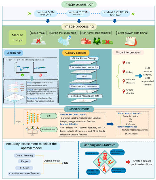
Figure 1.
Experimental flowchart.
2. Materials and Methods
2.1. Study Area Overview
The three provinces of China (Heilongjiang, Jilin, and Liaoning) considered in this study are located in the northeast of China, with geographic coordinates ranging from 40°N to 55°N and 120°E to 135°E (Figure 2). Most of the region has a temperate monsoon climate with relatively limited heat resources, and the mean annual temperature ranges from 2 °C to 6 °C. Precipitation is characterized by a clear rain–heat cycle, with obvious rain–heat synchronization characteristics, and is mainly concentrated in summer, with more rainfall in the southeast and less in the northwest in regard to spatial distribution. The total annual precipitation ranges from 500 to 800 mm. Forest ecosystems under this climate are vulnerable to extreme weather events (e.g., drought, high winds, heavy rainfall) [14]. The terrain is dominated by plains, hills, and mountains, and the land cover is dominated by woodlands, scrublands, and croplands, with abundant and concentrated forest resources. According to the latest data, the forest coverage rate is 43.78% for Heilongjiang Province, 41.49% for Jilin Province, and 39.24% for Liaoning Province. There is a variety of forest types, mainly including coniferous forests (e.g., red pines and larch), mixed coniferous and broadleaf forests, and deciduous broadleaf forests, with significant changes in the dynamics of forests in the region. In terms of natural factors, under the influence of a monsoon climate, forest fires (especially in spring and fall) are an important source of natural disturbances in the region; at the same time, wind-driven disasters caused by strong convective winds, heavy precipitation, secondary disasters, and pest outbreaks occur from time to time in the region [15,16]. As for anthropogenic activities, as a traditional forest management area, forest harvesting (including commercial logging and nursery logging) is the main anthropogenic activity that changes the forest cover, while the construction of roads in the forest area, the expansion of the edge of agricultural reclamation [17,18], the development of minerals, and the construction of tourism infrastructure also affect the stability of the forested area to different degrees [19]. Therefore, this northeastern region has become a typical and important area for the study of forest disturbances and their type identification [17].
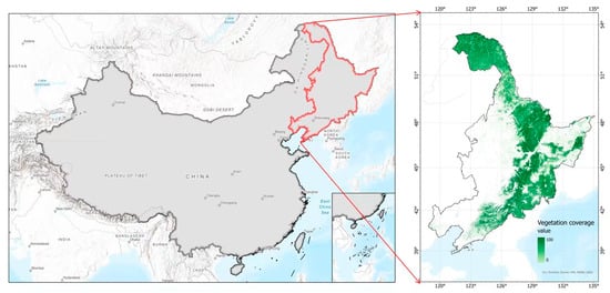
Figure 2.
Distribution map of forest land in Northeast China.
2.2. Data Sources and Preprocessing
2.2.1. Landsat 5/7/8 Data
Landsat series satellite data were acquired from the US Geological Survey (USGS) public archive platform (https://earthexplorer.usgs.gov/, accessed on 10 January 2025). The dataset includes Landsat 5 Thematic Mapper (TM) imagery (1984–2011), Landsat 7 Enhanced Thematic Mapper Plus (ETM+) imagery (1999–2022), and Landsat 8 Operational Land Imager/Thermal Infrared Sensor (OLI/TIRS) imagery (2013–2023) (Table 1), spanning the period 1984–2023 with a 30 m spatial resolution; these data cover the entire northeastern region. To minimize seasonal effects on vegetation signals, images between June 20 and August 10 were prioritized. Although the data were preprocessed by USGS and Google Earth Engine (GEE), additional cloud removal and masking were applied. The FMask algorithm was implemented to automatically mask clouds, cloud shadows, and snow, ensuring > 80% valid pixels per scene. Forest areas (coniferous, broadleaf, and mixed forests) were extracted, using the ESA Climate Change Initiative (CCI) Land Cover dataset (v2.0.7, 300 m resolution) as a mask template. This excluded non-forest disturbances (e.g., croplands, water bodies, and urban areas) from subsequent analyses.

Table 1.
Equivalent multispectral bands across Landsat sensors.
2.2.2. Auxiliary Datasets
(1) Global Forest Change [20]
This 30 m resolution dataset (2000–2022) from the University of Maryland comprises three layers: tree cover, forest loss, and forest gain. It was cross-validated with the Landsat data to identify long-term forest cover trends and served as a baseline for disturbance analysis.
(2) Tree cover loss due to fire [21]
The global 30 m resolution forest fire grids (University of Maryland) were used. Fire locations and timestamps within the study area (2001–2023) were extracted and integrated with Landsat temporal analysis to quantify the extent and intensity of fire-induced forest loss.
(3) Forest Pest and Disease Data
The Northeast China Forest Pest and Disease Dataset (2023) was integrated with field survey records of outbreak locations. Spatial analysis was conducted to delineate pest/disease disturbance impacts.
(4) LEAF [22]
The 30 m resolution Long-term HarvEst and Allocation of Forest Biomass (LEAF) dataset (Peking University) was processed to map harvesting locations and scales (2003–2018). Harvest-induced carbon dynamics were estimated through integration with forestry statistics.
(5) Geological Hazard Data
Spatial distributions of hazards (landslides, debris flows, collapses, and ground subsidence) were obtained from the National Geological Hazard Point Dataset (Geographical Remote Sensing Ecology Network). Only hazards intersecting the forested areas were retained.
The access links for the above datasets can be found in Appendix A.
2.2.3. Vegetation Index Calculation
To quantify changes in the state of forest ecosystems, the vegetation indices presented in Table 2 were calculated.
Table 2.
Comparison table of vegetation indices with their formulas and significance.
2.2.4. Multi-Source Validation Sample Construction
In this study, a multi-source sample construction method was used to construct a spatiotemporal validation framework on Google Earth Engine (GEE) by integrating LandTrendr image maps, Global Forest Change datasets, USGS global forest fire disturbance data, Peking University global change and terrestrial ecosystems disturbance datasets, and northeast region pest and disease thematic data. The dataset contains both disturbed and undisturbed samples. The selection process for disturbed samples specifically included multi-temporal visual interpretation, utilizing Landsat 5/7/8 historical image time-series (1992–2023), supplemented with Google Earth historical imagery, and combined with dynamic trajectory analysis to verify the type of disturbance. Each sample point must meet the evidence chain support of at least two independent years; quality control of the samples was conducted, and a three-level validation system was established (automatic screening → independent visual interpretation → verification of controversial sample dataset). Finally, 3100 validation samples were constructed, and their spatial distribution and sample category composition are shown in Table 3. The selection criteria for undisturbed samples were that no spectral change signals appeared in the long-term time-series, no disturbance records in the aforementioned auxiliary datasets, and no disturbance changes detected in the forest areas through visual interpretation. Ultimately, 2233 undisturbed samples were constructed.
Table 3.
Sample category composition.
2.3. Methodology
2.3.1. LandTrendr Algorithm
The LandTrendr algorithm is a forest disturbance detection method based on time-series segmented regression, which is capable of capturing sudden events (e.g., fire, logging) and long-term gradual processes (e.g., pests and diseases) of forest cover. In this study, we implemented the LandTrendr algorithm based on the Google Earth Engine (GEE) platform (Appendix C), and combined it with the time-series analysis of multiple vegetation indices to extract forest disturbance information from the study area. The core of the algorithm is to fit the vegetation index time-series via a segmented linear model to identify the sudden change points (breakpoints) and the gradual trend in forest cover [23].
The performance of the LandTrendr algorithm is highly dependent on the parameter settings, and this study identified the key parameters through pre-experimentation (Table 4).
Table 4.
LandTrendr model parameter settings.
2.3.2. Accuracy Verification of the LandTrendr Algorithm
The LandTrendr algorithm can effectively identify disturbed and undisturbed areas. We used 3100 sample points as validation data for disturbed areas and 2233 sample points as validation data for undisturbed areas. Because of potential minor positional discrepancies between these datasets and our field-measured data, we further expanded the calculated ranges for validation within the 30 m and 60 m buffer zones.
2.3.3. Random Forest and Deep Learning Classification Construction
Multidimensional Feature System
Based on Landsat spectral–temporal–spatial three-dimensional feature construction, blue (B1), green (B2), red (B3), near-infrared (B4), short-wave infrared 1 (B5), and short-wave infrared 2 (B7) bands [24], as well as NBR, EVI, NDVI, NDMI, SAVI, GNDVI, and MNDWI, were selected, together with ARVI and RVI feature indices, to form a multidimensional feature system.
Random Forest Model Architecture Design
This study constructed a random forest classification framework based on the GEE platform, and the model achieves the rapid identification and spatial mapping of forest disturbance types through the collaborative analysis of multi-source features and the integrated decision-making mechanism. The core components of the network architecture are as follows: In the feature optimization layer, 15-dimensional spectral index features (Landsat 6 bands + 9 vegetation indices) are fused together, and the significance of each index is determined and applied to the model for calculation. In the forest construction layer, 100 classification and regression trees (CART) are trained in parallel, with bootstrap resampling strategy for individual trees and random selection of feature subsets (m = ≈ 4). In the perturbation discrimination layer, the majority voting mechanism fuses the subtree prediction results and outputs four types of perturbation probability distributions. The model training parameters were set as shown in Table 5.
Table 5.
Model training strategy.
Feature importance was quantified using the Gini Importance method, which was implemented as the default feature_importances_ attribute in the RandomForestClassifier of the Scikit-learn library. This method accumulates the reduction in Gini impurity at all decision tree node splits, using the following formula:
whereindicates a feature, T is the number of trees, and n is the number of nodes. Feature importance is calculated using the default implementation in Scikit-learn, which is based on the average reduction in Gini impurity when splitting all tree nodes.
2.3.4. CNN Model Architecture Design
The study constructed a convolutional neural network (CNN) to accomplish the accurate recognition of forest disturbance types. The network architecture contains the following core components: A feature embedding layer that spatially maps 6-dimensional input features (Landsat 6 Bands) via a 32-channel convolutional kernel (kernel_size = 3). A feature abstraction layer that contains two convolutional modules, each consisting of convolutional layer → batch normalization → rectified linear unit (ReLU) activation → maximum pooling, with 32 → 64 channels. Global features are mapped to the category space through a fully connected layer (64 → 4). In the classification decision layer, the global average pooling is accessed by the fully connected layer (64 → 4), and SoftMax outputs four categories of perturbation probabilities that are mathematically expressed as follows:
wheredenotes the feature map of the lth layer, and BN is the batch normalization operation. A stratified random sampling strategy is used to divide the dataset (training set/test set = 8:2), and the key training parameters are as shown in Table 6.
Table 6.
CNN parameters. The pooling strategy of keeping the feature dimensions constant during model implementation can effectively avoid information loss under small sample data, and the fixed learning rate setting improves the stability of the training process.
2.4. Disturbance Magnitude Quantification
To comprehensively evaluate the overall intensity of disturbance for each pixel, a Synthetic Disturbance Magnitude Index (SDMI) was calculated. This index integrates information from four vegetation indices (NDVI, EVI, NDMI, and NBR) to avoid potential biases from any single index and to provide a robust one-dimensional measure. It was computed using the following formula:
where represents the synthetic disturbance magnitude value (dimensionless) for the pixel. represents the difference in the corresponding vegetation index value between the post-disturbance period and the pre-disturbance baseline period for the pixel. The notation indicates that the absolute value of the difference is taken. This ensures that changes in all indices are uniformly treated as a “deviation” from the normal state, thereby measuring the pure intensity and preventing signal cancelation that could occur if the responses of different indices were in opposite directions. The sum of the absolute differences is multiplied by 1000 to scale the result into an integer value for easier handling and interpretation. The final division by 4 calculates the arithmetic mean of the absolute change magnitudes from the four indices, resulting in a single, synthetic measure of disturbance intensity. A higher value indicates a stronger overall disturbance to the pixel’s vegetation across multiple dimensions, including greenness, biomass, water content, and burn severity.
2.5. Verification Methods and Parameters
To estimate the accuracy of forest disturbance extraction, an analytical method combining multiple vegetation indices with different buffer distances was applied. The confusion matrix (including four indicators: true positive (TP), false positive (FP), false negative (FN), and true negative (TN)) and five indicators derived from the confusion matrix (accuracy, user accuracy (UA), producer accuracy (PA), F1 score, and Kappa) were used for evaluation. To estimate the accuracy of forest disturbance classification, the predicted results were compared with the validation dataset, with the results’ accuracy estimated using four indicators: UA, PA, accuracy, and Kappa. In the confusion matrix, TP refers to the number of samples correctly predicted as positive by the model, FP refers to the number of samples incorrectly predicted as positive, FN refers to the number of samples incorrectly predicted as negative, and TN refers to the number of samples correctly predicted as negative. Additionally, accuracy refers to the proportion of correct predictions out of all predictions, which measures the overall correctness of the model. Its formula is
UA refers to the proportion of correctly predicted positive samples among all samples predicted as positive, measuring the model’s “precision.” The formula is
PA refers to the proportion of actual positive samples that the model correctly predicts, measuring the model’s ‘coverage’. The formula is
The F1 score is a comprehensive metric that can better reflect the true performance of the model. Its formula is
Kappa is used to measure the consistency between the classification results and actual outcomes, taking into account the agreement that may occur by random chance. The formula is
where N = TP + FP + FN + TN.
3. Results
3.1. Forest Disturbance Extraction
The NBR, EVI, NDVI, and NDMI time-series calculated from Landsat images from 1992 to 2023 were imported into the GEE platform, and clouds, snow, water bodies, and non-forested areas were masked. Segmented linear models of the four vegetation indices were fitted to each pixel, and the locations of the breakpoints and the magnitude of changes were detected. The dates were restricted to the period from June 20 to August 10 of each year (forest growing season), and finally Mann–Whitney U (MMU) filtering was performed to minimize the effect of noise. The results are shown in Figure 3.
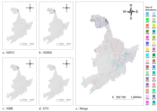
Figure 3.
LandTrendr calculation results. The combined map (Figure 3e) was obtained by taking the union of four vegetation indices (NDVI, NDMI, NBR, and EVI).
Using the vegetation index images fitted by the LandTrendr algorithm, it can be seen that although the perturbation areas and times based on the four vegetation indices are approximately the same, there are still some areas with different values for these indices, indicating different perturbation results. In the undisturbed areas, the values of the four indices are approximately the same, reflecting a normal vegetation growth pattern. In the disturbed areas, however, the vegetation indices show significant abrupt changes. This indicates that different vegetation indices present different recognition results for different disturbance categories.
As shown in Table 7, the use of the LandTrendr algorithm in combination with the Kappa index for forest disturbance extraction achieved a Kappa coefficient of 0.83, indicating good extraction performance. Among the various indices, the NBR index yields good results for disturbance extraction. This index exhibits sensitivity to changes in soil moisture content, vegetation cover, and vegetation health. NDMI, as a construction index, demonstrates good identification capabilities for artificial construction land. Therefore, for areas that were previously covered by vegetation but later became construction land, NDMI has relatively outstanding identification capabilities.
Table 7.
Accuracy assessment of forest disturbance detection using various vegetation indices and buffer distances.
To mitigate the inherent sample selection bias and the edge effects of 30 m resolution imagery, we implemented a stratified sampling strategy. Sampling was conducted in the core area, and disturbed samples were limited to pixels within continuous disturbance patches. An additional exclusion was applied to the edge buffer zone, with undisturbed samples collected from areas more than 60 m beyond the disturbance boundary. This method significantly improved the accuracy of all indices (e.g., the NBR Kappa value increased from 0.73 to 0.81). This improvement validates two key observations: the spectral distinguishability between disturbed and undisturbed forest categories is significant, and this method effectively reduces mixed-pixel contamination at transition boundaries. Notably, the multi-indicator fusion method (MERGE) achieved peak performance (Kappa = 0.86), confirming LandTrendr’s reliability in disturbance characterization while maintaining spatial resolution.
3.2. Random Forest Disturbance Classification Results
3.2.1. Random Forest Model Accuracy
We developed a classification mapping framework based on the random forest algorithm on the Google Earth Engine platform. By integrating multi-source temporal features with geospatial analysis, we generated spatiotemporal distribution data and calculated the accuracy of the model in classifying forest disturbance types in the northeast region from 1992 to 2023 (Table 8).
Table 8.
RF model accuracy.
From Table 8, it can be seen that the random forest model achieves high accuracy in the classification of all types of forest disturbances. The F1 scores for fires, disasters, logging, and pests and diseases are all above 0.89, indicating the RF model is capable of recognizing these four types of disturbances. The producer accuracy and user accuracy are also above 0.88, demonstrating that the model’s performance in avoiding false alarms and omissions is excellent. The overall accuracy reaches 0.9186 and the Kappa coefficient is 0.8906, which further validates the reliability and stability of the model. Therefore, the RF model has good identification as well as illustrative capabilities for classifying forest disturbance categories.
3.2.2. Feature Importance Analysis
The feature importance ranking (Figure 4) shows that the NBR and SWIR2 (B7) bands contribute the most, confirming the unique sensitivity of this index to vegetation canopy structure damage and moisture loss during LandTrendr’s accuracy identification. NBR effectively amplifies spectral response differences in burned areas or areas subjected to severe disturbances by combining the ratio calculation of the moisture-sensitive SWIR2 band and the near-infrared band. When fires cause canopy destruction, SWIR2 reflectance significantly increases due to exposed bare soil (compared with the low reflectance of healthy vegetation), and NBR further reinforces this signal through standardized calculations. Notably, NBR not only captures rapid changes following sudden disturbances (such as fires) but also exhibits significant responsiveness to progressive vegetation dehydration caused by pests and diseases. This multi-sensitivity makes it a core indicator for disturbance identification, and the high contribution of the SWIR2 band precisely reflects the key physical significance of the NBR index—a comprehensive characterization of vegetation moisture content and soil/litter reflectance, as expressed by the following formula:
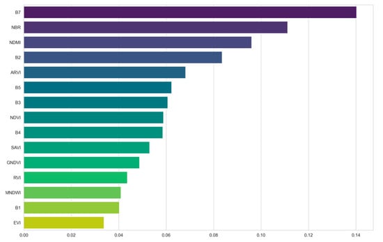
Figure 4.
Importance level of feature indices.
NBR is specifically designed for detecting fire disturbances [26], and its calculation formula emphasizes the contrast between SWIR and NIR bands. Severe disturbances (such as fires or clear-cutting) cause a sharp drop in NIR reflectance and an increase in SWIR2 reflectance, resulting in a significantly negative NBR value. Additionally, in previous LandTrendr accuracy validation studies, NDMI demonstrated excellent disturbance identification capabilities; in this study, NDMI also manifests strong disturbance classification capabilities. NDMI can effectively distinguish between construction land and bare land [27], as well as between construction land and forest land as the two exhibit distinct differences. If there is a change from forest land to construction land in the study area, it is typically identified by the random forest algorithm as an area affected by artificial logging disturbances. Furthermore, the contribution levels of the individual bands comprising NDMI are relatively high, which is of significant importance for this index’s high contribution rate.
Compared with the random forest algorithm using six original bands without vegetation index features (Table 9), the random forest algorithm with nine vegetation indices achieved even higher accuracy scores in all aspects.
Table 9.
RF (6-index) model accuracy.
3.3. CNN Model Performance Validation
3.3.1. Dynamic Analysis of the Training Process
Figure 5 shows the evolution of the loss function and classification accuracy of the CNN model over 200 training cycles (epochs). Both Train Loss and Test Loss in the left figure show an exponential decay trend, which is in line with the typical convergence law of deep learning models. This indicates the model’s early ability to quickly capture spectral features. After more training cycles, the decline rate slows down, the training/validation loss difference value always stays within 0.05, and the validation batch normalization (BatchNorm) effectively controls the risk of gradient explosion. It meets the expected convergence threshold of the CrossEntropyLoss function in the four-category classification task [28]. The training accuracy and validation accuracy in the right figure show synchronous improvement characteristics and eventually reach a steady state. The hyperbolic overlap is significantly improved after 150 cycles, confirming the model architecture design (32→64-channel convolution)’s ability to adequately fit the four types of perturbation features in the northeast region, with no over- and under-fitting phenomena.
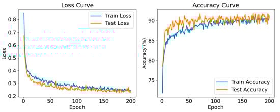
Figure 5.
Loss curve and accuracy curve of CNN.
The CNN model achieves an overall accuracy (OA) of 92.26% on the test set, with a Kappa coefficient of 0.8964. The confusion matrix shows an accuracy higher than 93.9% for the recognition of sudden disturbances (fires and geodetic disasters), and an accuracy higher than 89.6% for the classification of pest, disease, and logging disturbances (Table 10).
Table 10.
CNN model accuracy.
3.3.2. Feature Importance Analysis
The relative importance of the spectral features in the CNN classification model is illustrated in Figure 6 and Figure 7. The B7 (SWIR2) band exhibits the highest contribution to disturbance discrimination (indicated by its dominant horizontal axis length), significantly impacting all disturbance categories. Vegetation moisture absorption characteristics in the SWIR wavelengths enable this band to capture hydric stress variations across disturbance types. The B4 (Red) band’s utility arises from vegetation’s low reflectance in this spectral region, allowing it to sharply delineate forested from non-forested areas. Following geological disturbances (e.g., landslides or debris flows that cause large-scale forest destruction), the drastic reduction in vegetation cover produces pronounced reflectance increases in B4. Consequently, B4 exerts substantially greater influence on the CNN model’s geohazard classification decisions compared to other disturbance types.
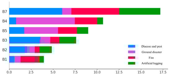
Figure 6.
Mean absolute SHAP (average impact magnitude on model output).
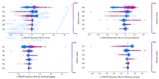
Figure 7.
SHAP values (impact on CNN model output).
3.4. Model Accuracy Comparison
Overall, through the deep mining of spectral–temporal features, the CNN model achieves an overall classification accuracy of 92.26% while maintaining high computational efficiency, which is better than traditional machine learning methods. The CNN algorithm and the random forest algorithm using 15 feature bands each have their own advantages for the classification of the four disturbance categories; the CNN has a significant advantage over the random forest algorithm in the recognition of forest fire disturbances (+ 2.3%), with the random forest algorithm being inferior to the CNN algorithm regardless of its use of the original feature bands or the 15 feature bands. The CNN algorithm also has an advantage (+0.75%) in recognizing forest disturbances caused by logging (Figure 8). In addition, we conducted significance tests on the three models. The results of the significance test analysis can be found in Appendix D.
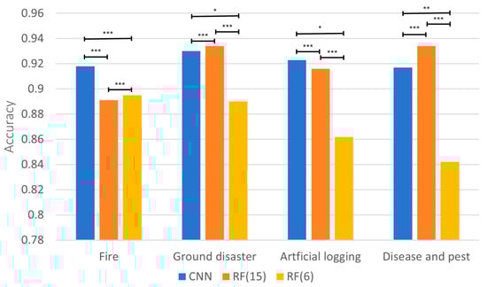
Figure 8.
Classification accuracy by category and method (* p < 0.05; ** p < 0.01; *** p < 0.001).
Compared with the CNN model, the overall accuracy of the random forest model is 2.3% lower, but it has the following advantages for applications: Random forest is ahead of CNN in the recognition and classification accuracy of pest and disease disturbances as well as geodetic disturbances, and its computational efficiency is high, while the time required for the classification of the whole region and the whole year is much lower than that of deep learning algorithms. RF has good interpretability and provides quantitative indicators of feature importance to support the analysis of ecological mechanisms. It has strong platform compatibility, can be directly integrated into the GEE cloud computing framework, and supports dynamic update (Figure 9).
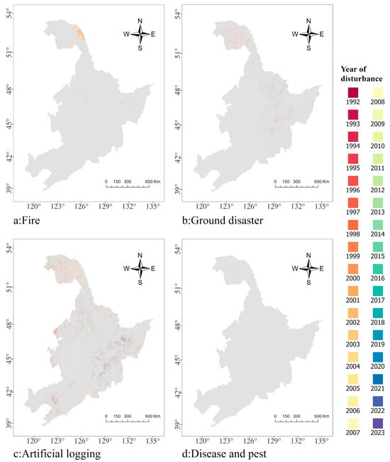
Figure 9.
Disturbance category and distribution.
3.5. Verification of Typical Disturbance Event Years
To verify the disturbance classification results of different years more clearly, this study reimported the classification images into the GEE platform for visual verification and extracted satellite images of disturbance events from them with obvious recognition effects (Figure 10). It was found that different indices could recognize different types of disturbances with different focuses, among which the B7 and NBR indices were more sensitive to fire, pest, and ground disturbances, but B7 was not effective in detecting clearcutting disturbances; the NBR indices, although they could recognize all four types of disturbances, were weaker than B7 for fire, pest, and ground disturbance and weaker than EVI and NDVI for clearcutting disturbances.
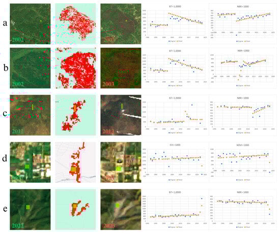
Figure 10.
Algorithm identification of regions subjected to disturbance events and actual images of these regions. The first row (a) shows the Huma River region (fire disturbance); the second row (b) shows the northern Greater Khingan Range region (fire disturbance); the third row (c) shows the Fusong County region (geological disaster disturbance); the fourth row (d) shows the Harbin region (logging disturbance); the fifth row (e) shows the Fushun City region (pest and disease disturbance). The first column shows the Landsat true-color composite imagery before the disturbance; the second column shows the detection results; the third column shows the imagery of the disturbance event. The horizontal axis in the graph represents year.
Meanwhile, the forest disturbance types in different areas had their unique spectral trajectories and time-series characteristics. For example, fire disturbances in the Huma River area and the northern part of the Greater Khingan Mountains showed significant changes in the vegetation indices before and after the disturbance, and the NBR and B7 indices were able to better reflect the degree and extent of fire damage to vegetation. The changes in the vegetation indices due to ground disturbances in Fusong County were closely related to the topographic conditions and soil stability, and the location and influence range of ground disturbances could be effectively identified by analyzing the abnormal changes in these indices. Regarding logging disturbances in Harbin area, the EVI and NDVI indices performed well in detecting the changes in vegetation cover and were able to accurately distinguish between logged and unlogged areas. In Fushun City, the changes in the vegetation indices exhibited a certain progressive nature due to disturbance caused by pests and diseases, and the NBR index was able to capture the water loss and spectral response changes in vegetation in the process of pest and disease infestation, providing a basis for early monitoring and control of pests and diseases.
4. Discussion
This study integrated the LandTrendr algorithm with a CNN model to achieve high-precision classification of four types of forest disturbances (fire, pests and diseases, geological disasters, and human logging) in Northeast China, with an overall accuracy of 92.26%. The study found that different disturbance types exhibit significant differences in vegetation index responses, terrain distribution, and time-series characteristics, outperforming traditional methods and providing important evidence for regional forest management and carbon cycle research.
4.1. Terrain Gradient and Disturbance Distribution
To robustly assess the intensity of identified disturbances, we employed the synthetic disturbance magnitude index () introduced in the Methods. This integrated measure, reflecting consolidated changes across four vegetation indices, revealed a clear gradient of disturbance strength across the study area (Table 11).
Table 11.
Correlation between disturbance amplitude and slope.
Table 11 shows that the four types of disturbances exhibit significant differences across different slope zones (Table 11). The four major forest disturbances (logging, fires, geological disasters, and pests and diseases) all exhibit larger disturbance amplitudes in flat areas with slopes <5°. This finding may reflect the unique vulnerability characteristics of forest ecosystems in flat areas. Concerning logging activities, the disturbance amplitude value of 380.88 in flat areas is significantly higher than in other slope zones. This is primarily due to the fact that flat terrain facilitates mechanized logging operations and transportation activities, resulting in a significant increase in the intensity and frequency of human disturbances [29]. Fire disturbances also reach the highest value (425.25) in flat areas, which is related to the increased number of fire sources caused by frequent human activities while also reflecting the greater accumulations of combustible materials in flat areas [30]. Although the disturbance amplitudes in flat areas are the highest overall, significant differences still exist in regard to the topographic gradient characteristics of different types of disturbances. Geological disasters are the only disturbance type showing a monotonically increasing trend, with their magnitude increasing to 198.79 in steep slope areas, clearly demonstrating the positive promotional effect of increased slope on geological disasters [31].
Fire disturbances exhibit a notable secondary peak (397.09) in the 10–15° slope zone, potentially related to the unique wind speed and combustible material distribution conditions in moderately sloped areas [32]. Pest and disease disturbances show an unusually high value (207.91) in the 35–45° slope zone—a phenomenon that may reflect the unique vegetation community structure and limited pest control efforts in this slope zone [33]. These findings have important implications for forest management. For example, fire prevention measures should be strengthened in moderately sloped areas, while geological hazards should be prioritized in steeply sloped areas. The results of this study also point the way for future research, particularly the need to further explore the impact of microtopographic features on disturbance processes and to develop more refined slope correction algorithms to improve monitoring accuracy in steeply sloped areas.
4.2. Ecological and Management Implications
This study is the first to quantify the spatiotemporal patterns of various types of disturbances in temperate forests in Northeast China at the regional scale. High-precision fire detection provides a data foundation for fire classification, while the concentration of logging hotspots in flat areas and urban regions reveals the indirect impact of urbanization on forest carbon storage. Additionally, the high incidence of geological disasters in steeply sloped areas (area proportion increases by 35% when the slope exceeds 45°) underscores the need to strengthen mountain protection engineering. From a methodological perspective, the CNN model outperforms the multi-feature random forest model (15 bands) even with limited features (only 6 bands), confirming the potential of deep learning in remote sensing time-series analysis.
Higher-precision forest disturbance extraction and classification methods provide a theoretical foundation for elucidating disturbance–recovery ecological mechanisms, exploring the quantification and interactions of driving factors, and revealing disturbance differentiation patterns and identifying disturbance factors (Figure 8). For example, this study found that high-incidence fire zones are concentrated in the Greater Khingan Range, which is closely related to the region’s continental arid climate and lightning-induced fire sources; pest outbreak hotspots are commonly found in artificial forests in Liaoning/Jilin, confirming the conclusion that single-species forests are more susceptible to invasion [34]; and logging hotspots are distributed along roads and urban networks, suggesting urbanization effects and human logging risks [35]. These findings provide a scientific basis for carbon management: fires lead to rapid carbon release (consistent with the LEAF dataset), while insect pest disturbances manifest as a sustained decline in carbon sink capacity. This is crucial for refining regional carbon budgets under the IPCC framework.
4.3. Methodological Advances and Comparative Performance
The LandTrendr-CNN collaborative method proposed in this study integrates temporal trajectory analysis with deep learning technology, fully leveraging the temporal feature extraction advantages of the LandTrendr algorithm and the spatial feature extraction advantages of the CNN algorithm [36]. This approach achieves higher classification accuracy compared to previous studies that used single temporal models or traditional machine learning methods for forest disturbance monitoring. When compared specifically with the widely used Hansen Global Forest Change (GFC) dataset, which identifies general forest loss without distinguishing disturbance types, our method demonstrates a significant advantage in classifying specific disturbance types. The study shows that the overall classification accuracy for the four types of forest disturbances (fires, pests and diseases, geological disasters, and human logging) achieved using this method reaches 92.26%, thus outperforming the Hansen Global Forest Change dataset (81.4%), and accuracy is also improved by 5.16% when compared with the random forest (RF) model under the same input features. This superior performance highlights the value of our approach for applications requiring detailed information on disturbance types. This result fully validates the effectiveness of the hybrid method of “time-series analysis + deep learning” in the field of remote sensing in recent years [37].
The core innovations of this method include the proposal of a multidimensional index combination of NDVI, NBR, EVI, and NDMI, which can efficiently distinguish forest disturbance types with different temporal characteristics, such as gradual (e.g., pest infestation) and sudden (e.g., fire) disturbances. The NBR and SWIR2 band (B7) have been proven to be key features (Figure 4 and Figure 6), effectively highlighting their sensitivity to vegetation structure loss, while also validating the findings of Kennedy [8] and Meng [38]. Unlike RF, which relies on manually constructed indices, CNN directly extracts spectral–spatial features from Landsat bands. Its advantages in detecting fires (F1 score +2.3%) and logging (+0.75%) highlight its ability to capture nonlinear disturbance features (e.g., the SWIR band’s response to bare soil after a fire) [39].
4.4. Limitations and Directions for Improvement
This study has the following limitations:
(1) Limitations in the judgment of visual interpretation samples: the validation sample construction relies on multi-temporal visual interpretation, but manual interpretation is subject to subjective errors. Early samples from 1992 to 2002 rely on Landsat 5 TM imagery (spatial resolution of 30 m), which has generational differences in radiometric calibration accuracy compared to Landsat 8 OLI, potentially introducing visual interpretation biases. Improvements could include introducing a cross-validation mechanism involving multiple interpreters and combining high-resolution historical aerial photographs (such as CORONA KH-4B imagery with a resolution of 1.8 m) for high-precision interpretation.
(2) The impact of cloud and fog disturbances on temporal continuity. Although the FMask cloud mask algorithm was used [40], the average annual cloud cover in the northeastern region is high (June–October), resulting in fewer than five effective observations per year in some years. This may result in increased false negatives for certain disturbances (e.g., pine needle pests) when using the LandTrendr algorithm. Multi-source temporal features can be constructed by integrating Sentinel-1 SAR data (C-band penetrates clouds) [41], and polarization features (VV/VH) can be used to enhance disturbance signal extraction capabilities during cloudy seasons.
(3) The classification of rare disturbance types is challenging. Due to the insufficient samples and limited visual interpretation capabilities of observers, this experiment could not further classify geological disaster disturbances (e.g., mudslides, collapses, landslides). Additionally, this experiment did not deeply explore the causes of geological disaster-induced forest disturbances, such as extreme temperatures, extreme precipitation, or human construction activities. It also lacks the ability to identify certain meteorological disasters, such as wind disasters or flood disasters, and requires the integration of multi-source data, such as precipitation data or temperature change data, for auxiliary identification to achieve better recognition of disturbance types and higher classification accuracy.
5. Conclusions
To achieve the accurate classification of multiple forest disturbance types, this study developed a novel forest disturbance classification and monitoring framework, integrating remote sensing data with deep learning technology. It achieved high-precision separation of four disturbance factors—fires, pest infestation, geological disasters, and human logging—in China’s northeast temperate forest region for the first time. By integrating the LandTrendr time-series analysis algorithm with a CNN deep learning model, the framework significantly improved the spatiotemporal accuracy of forest disturbance monitoring at the regional scale. The core contribution lies in quantifying disturbances by identifying specific reference disturbance areas and time points. Human-induced disturbances and natural disturbances exhibit significant differences, and classification facilitates carbon responsibility allocation. Additionally, the parameter system we developed (e.g., LandTrendr segment count, CNN convolution kernel) can be adapted to similar ecological regions in Northeast Asia (e.g., the Russian Far East), enabling transferable applications and contributing to regional ecological security. This study provides a feasible method and basic data for the refined management of temperate forest ecosystems and research on responses to global change. The model framework is scalable and has real-time platform functionality. We believe that this framework has the potential to achieve real-time, automated, and intelligent forest disturbance monitoring, supporting the scientific assessment of carbon neutrality goals in Northeast China’s forest regions.
Author Contributions
Conceptualization, Y.Y.; methodology, Z.Z. and Z.H.; software, X.Y. (Xinyi Yuan); validation, Y.Y. and Z.H.; formal analysis, Z.Z., X.Y. (Xiguang Yang), and X.Y. (Xinyi Yuan); investigation, Z.Z. and X.Y. (Xinyi Yuan); resources, X.Y. (Xiguang Yang); data curation, Z.Z.; writing—original draft preparation, Z.Z.; writing—review and editing, Y.Y. and X.Y. (Xiguang Yang); visualization, X.Y. (Xinyi Yuan); supervision, Y.Y.; project administration, Y.Y. and X.Y. (Xiguang Yang); funding acquisition, Y.Y. All authors have read and agreed to the published version of the manuscript.
Funding
This research was funded by the national key research and development program of the “14th five-year plan” project annual update technology of forest resource data based on multi-source data collaboration (2023YFD2201704), and the National Undergraduate Innovation and entrepreneurship training program (202410225297).
Data Availability Statement
The raw data supporting the conclusions of this article will be made available by the authors upon request.
Acknowledgments
The author acknowledges the providers of the following datasets: global forest loss due to fire (https://glad.umd.edu/dataset/Fire_GFL/, access on 10 January 2025), Global Forest Change (https://earthenginepartners.appspot.com/science-2013-global-forest, access on 10 January 2025), geological hazard dataset (www.gisrs.cn, access on 10 January 2025), and LEAF(https://www.nesdc.org.cn/sdo/detail?id=6656e3b17e28172539d2b90e, access on 10 January 2025). During the preparation of this manuscript, the authors used DeepL (https://www.deepl.com/zh/translator, access on 10 January 2025) for the purposes of translation and proofreading. The authors have reviewed and edited the manuscript and take full responsibility for the content of this publication. At the same time, the authors extend gratitude to all reviewers and editors who provided constructive suggestions for this article, offering invaluable assistance in its refinement.
Conflicts of Interest
The authors declare no conflicts of interest.
Abbreviations
The following abbreviations are used in this manuscript:
| NBR | Normalized Burn Ratio |
| EVI | Enhanced Vegetation Index |
| NDVI | Normalized Difference Vegetation Index |
| NDMI | Normalized Difference Moisture Index |
| ARVI | Atmospherically Resistant Vegetation Index |
| GNDVI | Green Normalized Difference Vegetation Index |
| MNDWI | Modified Normalized Difference Water Index |
| RVI | Ratio Vegetation Index |
| SAVI | Soil-Adjusted Vegetation Index |
| VCT | Vegetation Change Tracker |
| BFAST | Breaks for Additive Season and Trend |
| CCDC | Continuous Change Detection and Classification |
| CMFDA | Continuous Monitoring of Forest Disturbance Algorithm |
| LandTrendr | Landsat-based Detection of Trends in Disturbance and Recovery |
Appendix A
The website addresses of the four datasets used in this article are as follows:
Global forest loss due to fire (https://glad.umd.edu/dataset/Fire_GFL/, access on 10 January 2025).
Global Forest Change (https://earthenginepartners.appspot.com/science-2013-global-forest, access on 10 January 2025).
Geological hazard dataset (www.gisrs.cn, access on 10 January 2025), provided by Geographic remote sensing ecological network platform.
LEAF (https://www.nesdc.org.cn/sdo/detail?id=6656e3b17e28172539d2b90e, access on 10 January 2025)
Appendix B
Based on existing research, numerous mature and successful algorithms have been developed for monitoring forest disturbances using remote sensing satellite data, such as VCT, BFAST, CCDC, CMFDA, and LandTrendr. These algorithms possess distinct advantages and disadvantages, which determine their varying applicability. Table A1 lists the names, principles, advantages, and disadvantages of different algorithms.
Table A1.
Advantages and disadvantages of remote sensing time-series change detection algorithms.
Table A1.
Advantages and disadvantages of remote sensing time-series change detection algorithms.
| Algorithm | Advantages | Disadvantages |
|---|---|---|
| VCT | 1. Low computational complexity, enabling high automation through threshold-based methods. 2. Suitable for monitoring large-scale forest changes. 3. Strong robustness, insensitive to relatively poor observation points. | 1. Slow forest disturbances, such as pest infestations, are difficult to detect. 2. Sensitive to noise, resulting in proneness to misclassification. 3. Sensitive to consecutive anomalous observation points, resulting in proneness to misclassification. |
| BFAST | 1. Capable of simultaneously capturing both high-intensity and gradual disturbances. 2. Enables large-area change detection using multiple data sources. 3. Highly robust, while minimizing noise interference. | 1. Computationally complex, requiring high-performance computing hardware. 2. Poor performance in processing low-frequency data. 3. Limited detection capability for regions with repetitive disturbances. |
| CCDC | 1. Real-time monitoring capability. 2. High classification accuracy, capable of processing imagery with complex terrain types. 3. Multi-dimensional approach, enabling calculations that integrate spectral and seasonal information. | 1. High complexity, requiring substantial computational resources and extended processing time. 2. High-quality input data required, necessitating rigorous preprocessing of remote sensing imagery. 3. Sensitive to noise, as significant noise levels can compromise result accuracy. |
| CMFDA | 1. Multi-source data fusion captures information across different scales for computation. 2. Capable of detecting low-intensity forest disturbances, such as small-scale logging and pest infestations. 3. Suitable for complex geological and topographical environments with intricate surface features. | 1. High computational complexity and substantial processing demands. 2. Advanced programming skills required for model training. 3. High-quality input imagery required, with rigorous radiometric calibration. |
| LandTrendr | 1. Capable of simultaneously detecting disturbance trends and disturbance years. 2. Suitable for large-scale, long-term sequence monitoring. 3. Capable of simultaneously detecting multiple disturbance types. | 1. Limited capability to monitor small-scale disturbances. 2. Multiple adjustments to algorithm parameters required. 3. Processing large areas necessitates distributed computing support, imposing high demands on equipment. |
Table A2.
Descriptions of various deep learning algorithms.
Table A2.
Descriptions of various deep learning algorithms.
| Model Architecture | Core Principles | Main Advantages | Potential Applications in Forest Disturbance Classification |
|---|---|---|---|
| CNN | Specifically designed for processing grid-like data (such as images), CNN models automatically extract spatial features using convolutional kernels. | CNN models offer powerful spatial feature extraction capabilities, are relatively efficient in modeling, and are technically mature in image classification tasks. | CNN models can directly extract the spatial features of disturbance patches (such as shape, texture, and patterns) from remote sensing images, which can be employed to distinguish disturbances caused by fires, logging, and pests and diseases. |
| ResNet | A deep CNN that addresses the problem of vanishing gradients in very deep networks by incorporating residual connections (skip connections). | It can build extremely deep networks, thereby learning more complex features; training is more stable and performance is powerful. | Suitable for handling extremely complex or subtle perturbation features, it may provide higher classification accuracy when standard CNN performance is insufficient. |
| RNN/LSTM | Specifically designed to handle sequential data, it has a ‘memory’ function and can capture temporal dependencies. | Proficient in handling time-series data; capable of capturing the dynamic process of events and lag effects. | Suitable for analyzing long-term time-series vegetation indices (such as NDVI), capturing the occurrence, duration, and recovery dynamics of disturbances, and helpful in distinguishing disturbance types with different temporal trajectories. |
| GCN | Specifically designed to handle graph-structured data (non-Euclidean space), it learns and propagates information through node relationships. | Able to utilize spatial topological relationships and dependencies between entities. | Theoretically, it can be used to simulate the spatial correlation between disturbance patches in forest landscapes (such as the spread of pests and diseases), but data construction is complex, and its application is still in the exploratory stage. |
Appendix C
Oregon State University has established a system-level forest change monitoring algorithm (LandTrendr) on Google Cloud Platform. When utilizing this algorithm, users can simply call the corresponding code to activate it. Additionally, we have obtained a parameter-tuning UI interface (https://emaprlab.users.earthengine.app/view/lt-gee-pixel-time-series, access on 10 January 2025) that runs on the cloud platform. Users can access it with simple clicks or input operations to select parameters and regions of interest. Figure A1 below provides an overview of the UI interface.

Figure A1.
Landtrendr parameter adjustment UI interface.
Figure A1.
Landtrendr parameter adjustment UI interface.

Appendix D
Due to space constraints, we have presented the results of the significance tests in Table A3 and Table A4 below.
Table A3.
McNemar’s statistic values in the significance test results.
Table A3.
McNemar’s statistic values in the significance test results.
| McNemar’s Statistic | Fires | Ground Disasters | Artificial Logging | Diseases and Pests | Overall |
|---|---|---|---|---|---|
| RF15vsRF6 | 13.0 | 23.0 | 21.0 | 20.0 | 20.0 |
| RF15vsCNN | 9.0 | 17.0 | 8.0 | 12.0 | 11.0 |
| RF6vsCNN | 5.0 | 5.0 | 5.0 | 6.0 | 9.0 |
Table A4.
p-values in significance test results.
Table A4.
p-values in significance test results.
| p-Value | Fires | Ground Disasters | Artificial Logging | Diseases and Pests | Overall |
|---|---|---|---|---|---|
| RF15vsRF6 | 0.0000 | 0.0000 | 0.0000 | 0.0000 | 0.0000 |
| RF15vsCNN | 0.0000 | 0.0000 | 0.0000 | 0.0000 | 0.0000 |
| RF6vsCNN | 0.0266 | 0.0169 | 0.0169 | 0.0002 | 0.0000 |
References
- Chapin, F.S., III; Matson, P.A.; Vitousek, P.M. Principles of Terrestrial Ecosystem Ecology; Springer: New York, NY, USA, 2011. [Google Scholar]
- Liu, Y. The characteristics of radiation budget of earth atmosphere system over the Qinghai-Xizang Plateau and their relationship with climate change. Plateau Meteorol. 1998, 17, 37–44. [Google Scholar]
- Wu, L.; Liu, X.; Liu, M.; Yang, J.; Zhu, L.; Zhou, B. Online Forest Disturbance Detection at the Sub-Annual Scale Using Spatial Context from Sparse Landsat Time Series. IEEE Trans. Geosci. Remote Sens. 2022, 60, 4507814. [Google Scholar] [CrossRef]
- Huang, C.; Goward, S.N.; Masek, J.G.; Thomas, N.; Zhu, Z.; Vogelmann, J.E. An Automated Approach for Reconstructing Recent Forest Disturbance History Using Dense Landsat Time Series Stacks. Remote Sens. Environ. 2010, 114, 183–198. [Google Scholar] [CrossRef]
- Verbesselt, J.; Hyndman, R.; Newnham, G.; Culvenor, D. Detecting trend and seasonal changes in satellite image time series. Remote Sens. Environ. 2010, 114, 106–115. [Google Scholar] [CrossRef]
- Zhu, Z.; Woodcock, C.E. Continuous Change Detection and Classification of Land Cover Using All Available Landsat Data. Remote Sens. Environ. 2013, 144, 152–171. [Google Scholar] [CrossRef]
- Zhu, Z.; Woodcock, C.E.; Olofsson, P. Continuous monitoring of forest disturbance using all available Landsat imagery. Remote Sens. Environ. 2012, 122, 75–91. [Google Scholar] [CrossRef]
- Kennedy, R.E.; Yang, Z.; Cohen, W.B. Detecting Trends in Forest Disturbance and Recovery Using Yearly Landsat Time Series: 1. LandTrendr—Temporal Segmentation Algorithms. Remote Sens. Environ. 2010, 114, 2897–2910. [Google Scholar] [CrossRef]
- Chen, X.; Zhao, W.; Chen, J.; Qu, Y.; Wu, D.; Chen, X. Mapping Large-Scale Forest Disturbance Types with Multi-Temporal CNN Framework. Remote Sens. 2021, 13, 5177. [Google Scholar] [CrossRef]
- Yahya, A.A.; Liu, K.; Hawbani, A.; Wang, Y.; Hadi, A.N. A Novel Image Classification Method Based on Residual Network, Inception, and Proposed Activation Function. Sensors 2023, 23, 2976. [Google Scholar] [CrossRef]
- Wu, T.; Feng, F.; Lin, Q.; Bai, H. Advanced Method to Capture the Time-Lag Effects between Annual NDVI and Precipitation Variation Using RNN in the Arid and Semi-Arid Grasslands. Water 2019, 11, 1789. [Google Scholar] [CrossRef]
- Vasilakos, C.; Tsekouras, G.E.; Kavroudakis, D. LSTM-Based Prediction of Mediterranean Vegetation Dynamics Using NDVI Time-Series Data. Land 2022, 11, 923. [Google Scholar] [CrossRef]
- Pei, H.; Owari, T.; Tsuyuki, S.; Zhong, Y. Application of a Novel Multiscale Global Graph Convolutional Neural Network to Improve the Accuracy of Forest Type Classification Using Aerial Photographs. Remote Sens. 2023, 15, 1001. [Google Scholar] [CrossRef]
- Peña-Gallardo, M.; Vicente-Serrano, S.M.; Camarero, J.J.; Gazol, A.; Sánchez-Salguero, R.; Domínguez-Castro, F.; El Kenawy, A.; Beguería-Portugés, S.; Gutiérrez, E.; De Luis, M.; et al. Drought Sensitiveness on Forest Growth in Peninsular Spain and the Balearic Islands. Forests 2018, 9, 524. [Google Scholar] [CrossRef]
- Wang, Y.; Jia, X.; Zhang, X.; Lei, L.; Chai, G.; Yao, Z.; Qiu, S.; Du, J.; Wang, J.; Wang, Z.; et al. Tracking Forest Disturbance in Northeast China’s Cold-Temperate Forests Using a Temporal Sequence of Landsat Data. Remote Sens. 2024, 16, 3238. [Google Scholar] [CrossRef]
- Wegler, M.; Kuenzer, C. Potential of Earth Observation to Assess the Impact of Climate Change and Extreme Weather Events in Temperate Forests—A Review. Remote Sens. 2024, 16, 2224. [Google Scholar] [CrossRef]
- Sheng, J.; Gao, X.; Zhang, Z. Sustainability of Forest Development in China from the Perspective of the Illegal Logging Trade. Sustainability 2023, 15, 12250. [Google Scholar] [CrossRef]
- Liu, S.; Wang, D.; Lei, G.; Li, H.; Li, W. Elevated Risk of Ecological Land and Underlying Factors Associated with Rapid Urbanization and Overprotected Agriculture in Northeast China. Sustainability 2019, 11, 6203. [Google Scholar] [CrossRef]
- Li, Q.; Yang, Y.; Zhang, W.; Zhang, L.; Hu, C. Effects of Forest Management and Drought Disturbance on Forest Net Primary Productivity in Three Northeastern Provinces from 2000 to 2022. Bull. Soil Water Conserv. 2024, 44, 308–317. [Google Scholar] [CrossRef]
- Hansen, M.C.; Potapov, P.V.; Moore, R.; Hancher, M.; Turubanova, S.A.; Tyukavina, A.; Thau, D.; Stehman, S.V.; Goetz, S.J.; Loveland, T.R.; et al. High-Resolution Global Maps of 21st-Century Forest Cover Change. Science 2013, 342, 850–853. [Google Scholar] [CrossRef]
- Tyukavina, A.; Potapov, P.; Hansen, M.C.; Pickens, A.; Stehman, S.; Turubanova, S.; Parker, D.; Zalles, V.; Lima, A.; Kommareddy, I.; et al. Global trends of forest loss due to fire, 2001–2019. Front. Remote Sens. 2022, 3, 825190. [Google Scholar] [CrossRef]
- Wang, D.; Ren, P.; Xia, X.; Fan, L.; Qin, Z.; Chen, X.; Yuan, W. National forest carbon harvesting and allocation dataset for the period 2003 to 2018. Earth Syst. Sci. Data 2024, 16, 2465–2481. [Google Scholar] [CrossRef]
- Kennedy, R.E.; Yang, Z.; Gorelick, N.; Braaten, J.; Cavalcante, L.; Cohen, W.B.; Healey, S. Implementation of the LandTrendr Algorithm on Google Earth Engine. Remote Sens. 2018, 10, 691. [Google Scholar] [CrossRef]
- Wulder, M.A.; White, J.C.; Loveland, T.R.; Woodcock, C.E.; Belward, A.S.; Cohen, W.B.; Fosnight, E.A.; Shaw, J.; Masek, J.G.; Roy, D.P. The global Landsat archive: Status, consolidation, and direction. Remote Sens. Environ. 2016, 185, 271–283. [Google Scholar] [CrossRef]
- Louppe, G. Understanding Random Forests: From Theory to Practice. arXiv 2014, arXiv:1407.7502. [Google Scholar]
- Liu, D.; Qu, Y.; Yang, X.; Zhao, Q. TSSA-NBR: A Burned Area Extraction Method Based on Time-Series Spectral Angle with Full Spectral Shape. Remote Sens. 2025, 17, 2283. [Google Scholar] [CrossRef]
- Zha, Y.; Gao, J.; Ni, S. Use of normalized difference built-up index in automatically mapping urban areas from TM imagery. Int. J. Remote Sens. 2003, 24, 583–594. [Google Scholar] [CrossRef]
- Bjorck, N.; Gomes, C.P.; Selman, B.; Weinberger, K.Q. Understanding batch normalization. arXiv 2018, arXiv:1806.02375. [Google Scholar] [CrossRef]
- Watson, J.E.M.; Evans, T.; Venter, O.; Williams, B.; Tulloch, A.; Stewart, C.; Thompson, I.; Ray, J.C.; Murray, K.; Salazar, A.; et al. The exceptional value of intact forest ecosystems. Nat. Ecol. Evol. 2018, 2, 599–610. [Google Scholar] [CrossRef]
- Elia, M.; Lafortezza, R.; Colangelo, G.; Sanesi, G. A streamlined approach for the spatial allocation of fuel removals in wildland–urban interfaces. Landsc. Ecol. 2014, 29, 1771–1784. [Google Scholar] [CrossRef]
- Qiu, H.; Cui, P.; Regmi, A.D.; Hu, S.; Wang, X.; Zhang, Y. The effects of slope length and slope gradient on the size distributions of loess slides: Field observations and simulations. Geomorphology 2018, 300, 69–76. [Google Scholar] [CrossRef]
- Hayajneh, S.M.; Naser, J. Wind and Slope Influence on Wildland Fire Spread, a Numerical Study. Fire 2025, 8, 217. [Google Scholar] [CrossRef]
- Ferrenberg, S. Landscape Features and Processes Influencing Forest Pest Dynamics. Curr. Landsc. Ecol. Rep. 2016, 1, 19–29. [Google Scholar] [CrossRef][Green Version]
- Bell, G.; Sena, K.L.; Barton, C.D.; French, M. Establishing Pine Monocultures and Mixed Pine-Hardwood Stands on Reclaimed Surface Mined Land in Eastern Kentucky: Implications for Forest Resilience in a Changing Climate. Forests 2017, 8, 375. [Google Scholar] [CrossRef]
- Tanveer, A.; Song, H.; Faheem, M.; Daud, A. Caring for the environment. How do deforestation, agricultural land, and urbanization degrade the environment? Fresh insight through the ARDL approach. Environ. Dev. Sustain. 2025, 27, 11527–11562. [Google Scholar] [CrossRef]
- Zhang, L.; Zhang, L.; Du, B. Deep Learning for Remote Sensing Data: A Technical Tutorial on the State of the Art. IEEE Geosci. Remote Sens. Mag. 2016, 4, 22–40. [Google Scholar] [CrossRef]
- Xie, G.; Liu, P.; Chen, Z.; Chen, L.; Ma, Y.; Zhao, L. Time Series Remote Sensing Image Classification with a Data-Driven Active Deep Learning Approach. Sensors 2025, 25, 1718. [Google Scholar] [CrossRef]
- Meng, R.; Dennison, P.E.; D’Antonio, C.M.; Moritz, M.A. Remote sensing analysis of vegetation recovery following short-interval fires in Southern California shrublands. PLoS ONE 2014, 9, e110637. [Google Scholar] [CrossRef] [PubMed] [PubMed Central]
- Wang, Z.; Yang, P.; Liang, H.; Zheng, C.; Yin, J.; Tian, Y.; Cui, W. Semantic Segmentation and Analysis on Sensitive Parameters of Forest Fire Smoke Using Smoke-Unet and Landsat-8 Imagery. Remote Sens. 2022, 14, 45. [Google Scholar] [CrossRef]
- Mateo-García, G.; Gómez-Chova, L.; Amorós-López, J.; Muñoz-Marí, J.; Camps-Valls, G. Multitemporal Cloud Masking in the Google Earth Engine. Remote Sens. 2018, 10, 1079. [Google Scholar] [CrossRef]
- Philipp, M.B.; Levick, S.R. Exploring the Potential of C-Band SAR in Contributing to Burn Severity Mapping in Tropical Savanna. Remote Sens. 2020, 12, 49. [Google Scholar] [CrossRef]


Disclaimer/Publisher’s Note: The statements, opinions and data contained in all publications are solely those of the individual author(s) and contributor(s) and not of MDPI and/or the editor(s). MDPI and/or the editor(s) disclaim responsibility for any injury to people or property resulting from any ideas, methods, instructions or products referred to in the content. |
© 2025 by the authors. Licensee MDPI, Basel, Switzerland. This article is an open access article distributed under the terms and conditions of the Creative Commons Attribution (CC BY) license (https://creativecommons.org/licenses/by/4.0/).