Article

Research on the Application of Atmospheric Motion Vector from MetOp Satellite Series in CMA-GFS

1
CMA Earth System Modeling and Prediction Centre (CEMC), China Meteorological Administration, Beijing 100081, China
2
State Key Laboratory of Severe Weather Meteorological Science and Technology (LaSW), China Meteorological Administration, Beijing 100081, China
*
Author to whom correspondence should be addressed.
Remote Sens. 2025, 17(21), 3519; https://doi.org/10.3390/rs17213519
Submission received: 22 August 2025 / Revised: 21 October 2025 / Accepted: 21 October 2025 / Published: 23 October 2025
(This article belongs to the Section Atmospheric Remote Sensing)

Highlights

What are the main findings?
  • This study has developed assimilation techniques encompassing quality control and thinning schemes for MetOp-Dual, MetOp-B and MetOp-C based on CMA-GFS (China Meteorological Administration Global Forecast System), which fills the gap in the application of such data in CMA-GFS.
  • MetOp AMV products, through quality control and thinning, have increased the AMVs in CMA-GFS by 25%. By effectively reducing the observational gaps in polar and oceanic areas, the one-month assimilation experiment of MetOp AMV improves CMA-GFS's backgrounds (particularly the polar and high-latitude regions) and advances the usable forecast lead time for global 500 hPa geopotential height by 0.22 days.
What are the implications of the main findings?
  • This study, for the first time, applies MetOp-Dual, MetOp-B and MetOp-C products in CMA-GFS, which significantly promotes the AMV data utilization rate in CMA-GFS.
  • The one-month assimilation experiment of MetOp AMV products significantly improves the model background and forecasting performance of the CMA-GFS, which implies the MetOp AMV products can play a positive role in promoting the forecast performance of the operational CMA-GFS in the long run.

Abstract

Atmospheric motion vector (AMV) products from EUMETSAT’s MetOp satellite series, including MetOp-B, MetOp-C, and the MetOp-B/C tandem (MetOp-Dual), have been assimilated at many numerical weather prediction centers worldwide. However, they have not yet been applied in the China Meteorological Administration’s Global Forecast System (CMA-GFS). This study addresses this gap by developing assimilation techniques, including quality control and thinning methods for MetOp AMVs. Based on these techniques, one-month assimilation and forecasting experiments reveal that MetOp AMVs increased the AMV volume in CMA-GFS by 25%, filling certain gaps over polar and oceanic areas. Notable and steady improvements in the background of CMA-GFS have been found, particularly in polar and high-latitude regions. The usable forecast lead time for the global 500 hPa geopotential height is extended by 0.22 days, enhancing the reliability of medium-range forecasts. Furthermore, the more substantial improvements in short-range (0–3 days) forecasting, potentially benefit severe weather alerting. This study marks the first to successfully apply MetOp-B, MetOp-C and MetOp-Dual products in CMA-GFS, confirming their value for improving the performance of the system.

1. Introduction

Atmospheric motion vectors (AMVs), derived by tracking cloud and water vapor images from meteorological satellites, are used to improve the initial wind fields in numerical models, thereby improving the performance of numerical weather forecasting [1,2,3,4,5,6]. With the development of meteorological satellites, AMV products have become indispensable for major numerical weather prediction centers worldwide [5,7]. Based on their orbits, AMV can be categorized into those from geostationary satellites, such as the European Meteosat series [8], the United States’ GOES series [9], Japan’s Himawari series [10], and China’s Fengyun series [11], as well as those from the polar-orbiting satellites such as the MetOp series [12], the NOAA series [13], the SNPP satellite [14], the Aqua satellite [15], and the Terra satellite [16].
MetOp, short for Meteorological Operational Satellite Program, is a collaboration effort between the European Space Agency (ESA) and the European Organisation for the Exploitation of Meteorological Satellites (EUMETSAT). Its aim is to provide satellite observations for weather prediction and climate monitoring [12]. The MetOp-A satellite was launched in 2006 and the MetOp-A AMV product has been generated continuously since then. The MetOp-B satellite was launched in 2012, with its AMV product also being produced continuously. Subsequently, the dual-satellite MetOp-Dual AMVs were generated through joint retrieval from the MetOp-A and MetOp-B satellites. These two satellites orbited in the same polar orbital plane but at different phases, which attaches two advantages to MetOp-Dual AMV over AMVs from a single polar-orbiting satellite: (1) The time interval between two consecutive satellite images is reduced from approximately 100 min to about 50 min, which lowers the uncertainties in AMV retrieval. (2) It provides global coverage by filling the gaps at latitudes 55–70° north and south that can hardly be covered by either geostationary or polar-orbiting satellite [12]. Following the launch of MetOp-C in 2018 and the retirement of MetOp-A in 2021, MetOp-Dual AMVs are now derived jointly from MetOp-B and MetOp-C instead of MetOp-A and MetOp-B. As of 2024, part or all of the AMV product from MetOp-B, MetOp-C, and MetOp-Dual has been assimilated in major international numerical weather prediction centers, such as the European Centre for Medium-Range Weather Forecasts (ECMWF) [13], the Meteorological Service of Canada [14], the Japan Meteorological Agency [15], the UK Met Office [17], and Météo-France [18], and this has proven beneficial.
The Global/Regional Assimilation and Prediction Enhanced System (GRAPES_GFS), developed by the China Meteorological Administration, is a global four-dimensional variational assimilation and forecasting system. It became fully operational in 2016 [19,20]. AMVs derived from China’s FengYun geostationary satellite series were subsequently utilized in GRAPES_GFS [21,22,23,24]. GRAPES_GFS was renamed CMA-GFS in 2023 and upgraded to version 4.2. With a horizontal resolution of 12.5 km, CMA-GFS has a usable forecast lead time exceeding 8 days in the Northern Hemisphere. Its precipitation forecasts are approaching those of the European Centre for Medium-Range Weather Forecasts (ECMWF) and United States National Centers for Environmental Prediction (NCEP) [25,26,27]. However, as of 2024, the application of AMV products from MetOp-B, MetOp-C, and MetOp-Dual in CMA-GFS remains unexplored.
Through preliminary research by the authors, it was found that the MetOp series can supplement observational gaps, where AMVs are blank or sparse in CMA-GFS. For instance, during the assimilation window of 15:00 to 21:00 UTC on 1 July 2024, geostationary AMVs such as those from FY-2G, FY-2H, GOES16, GOES18, Himawari-9, and METEOSAT-11 cover most of the mid- to low-latitude regions. However, certain gaps in the eastern Pacific and southeastern Atlantic Ocean (near Southern Africa) are found, while AMVs from MetOp-Dual can effectively fill these gaps (Figure 1). Moreover, in polar regions, AMVs from MetOp-B, MetOp-C, and MetOp-Dual complement existing observations from NOAA20 and SNPP, thereby enriching wind data in polar regions. Therefore, it can be concluded that there is significant potential for applying MetOp AMVs in CMA-GFS.
Effectively utilizing MetOp-B/C/Dual AMVs in CMA-GFS demands a customized assimilation scheme. Current practices, typically adapted from other systems, may not fit CMA-GFS’s unique characteristics. This limitation hinders the full exploitation of these observations. Our study addresses this gap by developing tailored assimilation techniques, specifically through the design of quality control and thinning schemes optimized for CMA-GFS. The impact of these innovations is then evaluated through one-month cyclic assimilation and forecasting experiments. The paper is organized as follows: Section 2 details the materials and methods; Section 3 introduces the preprocessing of MetOp series AMVs for assimilation, including the quality control scheme and thinning scheme; Section 4 examines the impact of MetOp series AMVs on the backgrounds and forecasts of CMA-GFS; and Section 5 gives the conclusion.

2. Materials and Methods

2.1. Data

MetOp series AMV products encompassing MetOp-B AMV, MetOp-C AMV and MetOp-Dual AMV are used in this study. The MetOp-B AMV product has been used from 2012 until now (2025). The MetOp-C AMV product has been used from 2018 until now (2025). The MetOp-Dual (MetOp-B/C tandem) product has been used from 2019 until now (2025). The MetOp-B and MetOp-C AMV datasets (MetOp-B/C atmospheric motion vectors: https://navigator.eumetsat.int/product/EO:EUM:DAT:0380 (accessed on 1 August 2025)), as well as the MetOp-Dual dataset (MetOp Dual atmospheric motion vectors: https://navigator.eumetsat.int/product/EO:EUM:DAT:0379 (accessed on August 2025)), are publicly accessible via the EUMETSAT Data Navigator. For our study, we obtain the data via the Tianqing platform, developed by National Meteorological Information Center from China that provides MetOp series AMV data operationally for model researchers within the China Meteorological Administration System.
MetOp-B AMV and MetOp-C AMV primarily cover polar regions, whereas MetOp-Dual AMV provides global coverage. All three types of AMVs are derived from the 10.8 μm infrared channel using the Advanced Very-High-Resolution Radiometer (AVHRR), with a horizontal resolution of 30.8 km. The calculation of AMV involves five steps [12]:
  • Target extraction;
  • Tracking;
  • Height assignment;
  • Derivation of the final vector;
  • Automatic quality control (AQC).
The third step, height assignment, primarily with the help of reanalysis data, is a major source of error in AMV derivation [12,28,29]. Therefore, the quality indicator (QI) is developed by the EUMETSAT to characterize the reliability of each data point. A smaller QI represents poorer data quality, while a QI of 100 signifies the best data quality.
ERA5 reanalysis data were used for quality control of MetOp AMV data before assimilation and to evaluate the analysis fields of CMA-GFS. ERA5 data have a horizontal resolution of 0.25° and 37 vertical layers from 1000 to 1 hPa [30].

2.2. Methods

The CMA-GFS model is the global medium-range numerical weather prediction system developed by China Meteorological Administration. It became fully operational in 2016 and was subsequently upgraded to versions 3.3 and 4.0 in 2022 and 2023, respectively. Through these upgrades, improvements have been made in data assimilation, dynamical frameworks, and physical processes, steadily enhancing forecast performance to approach international advanced levels [26,31]. The CMA-GFS4.2 has a horizontal resolution of 0.125° (approximately 12.5 km), 87 vertical levels with the model top at 0.1 hPa, and a forecast lead time of 10 days. Further details on model configuration can be found in the relevant literature [31]. Two one-month experiments were conducted to evaluate the impact of MetOp series AMVs in CMA-GFS:
  • Control Experiment: Based on CMA-GFS4.2, all currently operational data are assimilated, including ground in situ observations, radiosonde data, aircraft reports, radio occultation data, and satellite radiance data, to run cyclic assimilation and forecast from 15 June to 1 August 2024. The driving data were from NCEP (short for National Centers for Environmental Prediction) Global Data Assimilation System Final Operational Analysis (FNL).
  • Sensitivity Experiment: The settings are the same as those in the Control Experiment, except that MetOp-Dual, MetOp-B, and MetOp-C AMV data are added to the assimilation.
Considering that 10 days are required to compute and update satellite bias correction coefficients in the assimilation system, the comparison period for the Control Experiment and Sensitivity Experiments is set from 1 July to 1 August 2024.

3. Preprocessing of MetOp Series AMVs Before Assimilation

3.1. Quality Assessment and Quality Control

Quality control is an essential step for any data entering an assimilation system, aiming to eliminate poor-quality data to ensure assimilation performance. This subsection introduces the quality control scheme for MetOp-Dual AMV as a typical case for MetOp Series AMV quality control.
First, only samples with a quality indicator (QI) of 80 or higher are retained, while those below this threshold are excluded. This ensures the reliability of the assimilated AMV data.
Next, ERA5 wind data are used to assess the AMV data and establish selection criteria for high-quality AMV data. Specifically, ERA5 wind data from 18 February to 1 April 2023 are compared with AMV data for the same period. The comparison procedures are as follows: (1) Temporally, ERA5 data at 3 h intervals (00, 03, 06, 09, 12, 15, 18 UTC) are matched with AMV data within ±1.5 h. For example, AMV data between 01:30 and 04:30 are considered concurrent with ERA5 data at 03:00 UTC. (2) Spatially, ERA5 winds are bilinearly interpolated to the AMV sample positions. Based on the above spatio-temporal matching, the bias (bias) and root mean square error (RMSE) of AMV relative to ERA5 horizontal wind fields are calculated.
The comparison reveals systematic differences in wind components between MetOp AMVs and ERA5 reanalysis. For the zonal wind (U), the mean bias is −0.63 m/s with an RMSE of 2.94 m/s. The meridional wind (V) shows a smaller bias of −0.05 m/s and an RMSE of 2.88 m/s. When combined into horizontal wind speed, the overall bias is −0.30 m/s with an RMSE of 3.00 m/s (Figure 2a,b). These results indicate that the zonal wind component (U) constitutes the primary source of discrepancy between MetOp AMVs and ERA5.
Further analysis reveals that 99.1% of MetOp AMV observations record horizontal wind speeds below 30 m/s. When the comparison is restricted to this majority subset, the agreement with ERA5 improves substantially. The bias in horizontal wind speed decreases dramatically from −0.30 m/s to −0.03 m/s, while the RMSE drops from 3.00 m/s to 2.21 m/s (Figure 2b). These results demonstrate that excluding the small number (0.9%) of high-wind-speed samples (above 30 m/s) drastically reduces the discrepancy between MetOp AMVs and ERA5 reanalysis.
Statistics by altitude reveal that the number of MetOp AMVs generally decreases with height. The bias and RMSE values relative to ERA5 exhibit a pattern of increasing with height (Figure 3). Statistical results indicate that AMVs above 200 hPa account for only 0.8% of the total AMV volume. The bias and RMSE values above 200 hPa are 1.61 m/s and 5.5 m/s, respectively, while those below 200 hPa are −0.40 m/s and 3.7 m/s, respectively (Figure 3). This confirms that the bias and RMSE values for horizontal wind speeds above 200 hPa are much larger than those at lower levels.
Based on the above results, the differences between MetOp AMVs and ERA5 mainly come from a small number of high-altitude or high-wind-speed samples. Therefore, the following quality control scheme is proposed: retain samples with confidence levels above 80%, pressure levels below 200 hPa, and horizontal wind speeds less than 30 m/s, while excluding any samples that do not meet all these criteria.

3.2. Spatial Thinning Scheme

During data assimilation, it is assumed that observation errors at different locations are uncorrelated, but the correlation of observation errors is difficult to determine. Therefore, dense observational data must be thinned to minimize correlations in observation errors at different locations [32]. Previous spatial thinning schemes, often limited to the horizontal dimension, could result in the exclusion of data points that are horizontally close but vertically distant, which should be treated as distant points and not be discarded [28]. If those data are to be saved, a three-dimensional thinning scheme is preferable to a two-dimensional one. Based on these considerations, a three-dimensional thinning scheme with a horizontal interval of 200 km and a vertical interval of 50 hPa for MetOp-Dual AMVs is designed following existing thinning intervals [33]. Three-dimensional thinning scheme encompasses three steps, Create Thinning Anchors, Horizontal Thinning, and Vertical Thinning.
Step 1. Create Thinning Anchors.
The globe is divided into thinning anchors spaced approximately 200 km apart horizontally. The reason for creating these thinning anchors is that they are used to “attract” the closest AMV point from the swath of AMV observations, so that the attracted AMV points can be treated as ~200 km apart horizontally. The procedure is as follows.
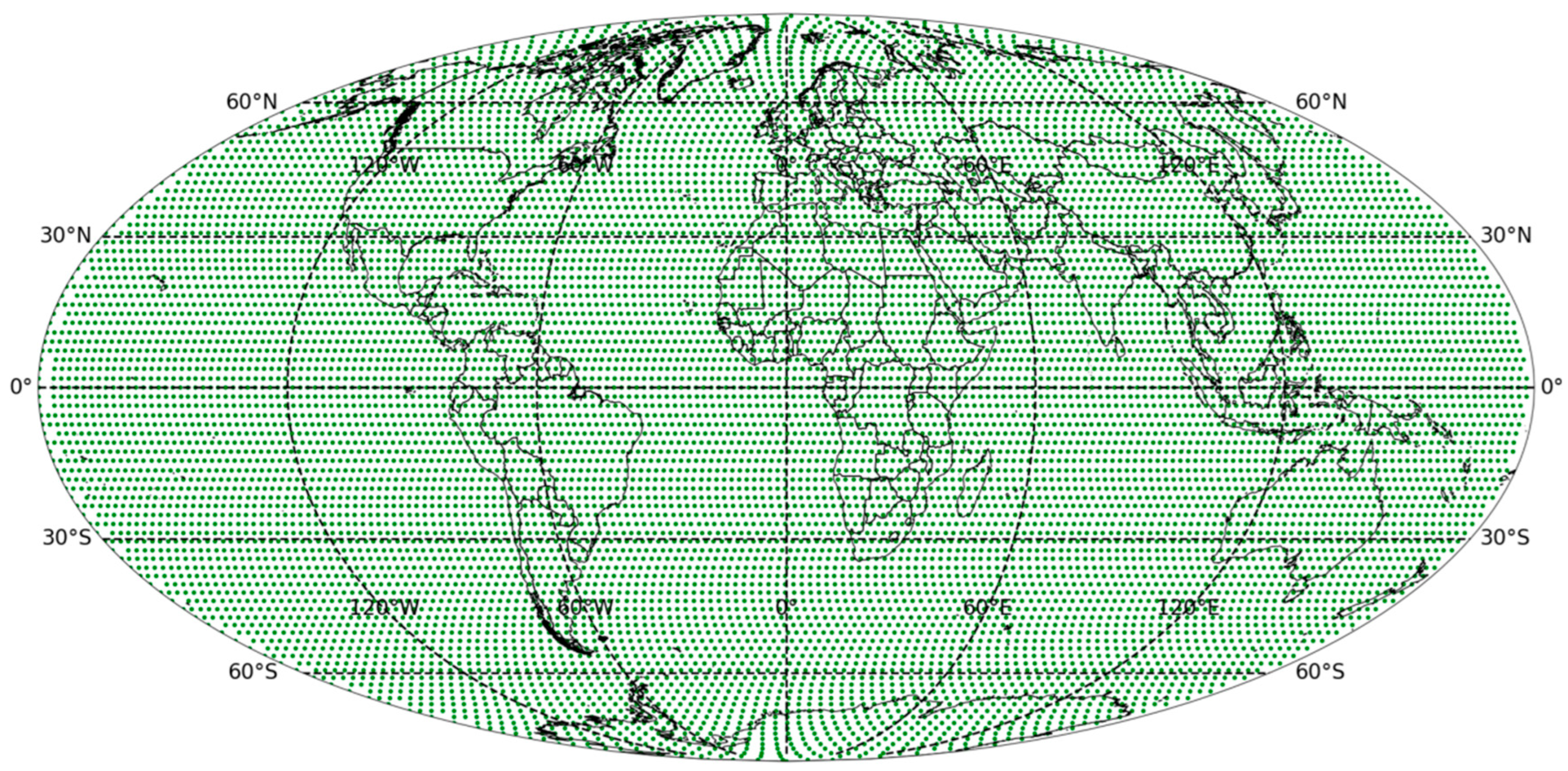
The globe is treated as a perfect sphere, and latitudes are divided at 200 km intervals from 90°S to 90°N along the meridians. For each latitude, the circumference of the latitude circle is divided at 200 km intervals to establish global anchors. If a strict 200 km interval cannot be maintained, it is adjusted to ensure that the distance between anchors is no less than 200 km. This process results in 12,634 global anchors with an average horizontal interval distance of ~200 km (Figure 4).
Step 2. Horizontal Thinning.
For a given assimilation time slot i, all MetOp-Dual AMVs that have passed quality control are collected. For each AMV observation point, the horizontal distance to its nearest anchor is calculated using the haversine formula (Equations (1)–(3)).
a = s i n 2 ϕ 2 + c o s ϕ 1 c o s ϕ 2 s i n 2 λ 2
c = 2 a t a n 2 ( a , 1 a )
d = R c
where ϕ 1 and ϕ 2 are the latitudes (in radians) of the observation point and the anchor point, ϕ and λ are the differences in latitude and longitude, respectively, R is the Earth’s radius (approximately 6371 km), and d  is the horizontal distance between the two points.
The anchors closest to all AMV observation points can then be identified. Since multiple observation points may be closest to the same anchor, duplicates are removed, resulting in a unique set of anchors, denoted as set A.
Step 3. Vertical Thinning.
For each anchor B in set A, all observation points that are horizontally closest to B are identified in order to form set C. Within set C, observation points have varying pressure levels. Starting from the point at the lowest-level pressure in set C, each subsequent observation is checked to ensure a vertical interval of at least 50 hPa from the previous one. Observations that do not meet this criterion are excluded, and the process continues upward to the top pressure level of set C to determine the final set of observations, set D, which meets both horizontal and vertical thinning criteria for anchor B. This process is repeated for all anchors in set A to obtain the thinned dataset E. In set E, adjacent observation points are ~200 km apart horizontally and more than 50 hPa apart vertically.
Notably, if only the horizontally closest observation to each anchor is retained without consideration of their vertical distance, the scheme reduces to two-dimensional thinning.
Statistical results for the half-hour assimilation time slot from 02:45 to 03:15 UTC on 25 May 2024 show that 4840 MetOp-Dual AMV observations have passed quality control. After two-dimensional thinning, 444 MetOp-Dual AMV observations were retained, a data retention rate of ~10% (Figure 5a). In contrast, three-dimensional thinning has retained 963 MetOp-Dual AMV observations, a retention rate of ~20% (Figure 5b). Meanwhile, the retention ratio of MetOp-B is 158/1930 in two-dimensional thinning and 360/1930 in three-dimensional thinning, respectively. The retention ratio of MetOp-C is 161/1723 in two-dimensional thinning and 341/1723 in three-dimensional thinning, respectively.
Thus, the three-dimensional thinning scheme nearly doubled the data retention compared to two-dimensional thinning, effectively enhancing CMA-GFS’s utilization of MetOp AMVs.
Therefore, this three-dimensional thinning scheme is applied to the MetOp AMV data after quality control.

4. Impact of MetOp Series AMVs on the Backgrounds and Forecasts of CMA-GFS

4.1. Increase in Assimilated Data Volume

The Sensitivity Experiment differs from the Control primarily through the inclusion of MetOp-series AMVs, which increase total AMV data by 25% (Figure 6a). These additional observations account for 20.1% of all AMVs, with particularly greater contributions in polar regions and the mid-troposphere. Specifically, MetOp AMVs constitute 41.1% of all AMVs between 500 and 600 hPa (Figure 6b). In polar latitudes (80–90°), they represent nearly 80% of AMVs between 400 and 600 hPa, substantially augmenting wind observations in these data-sparse regions (Figure 6c).
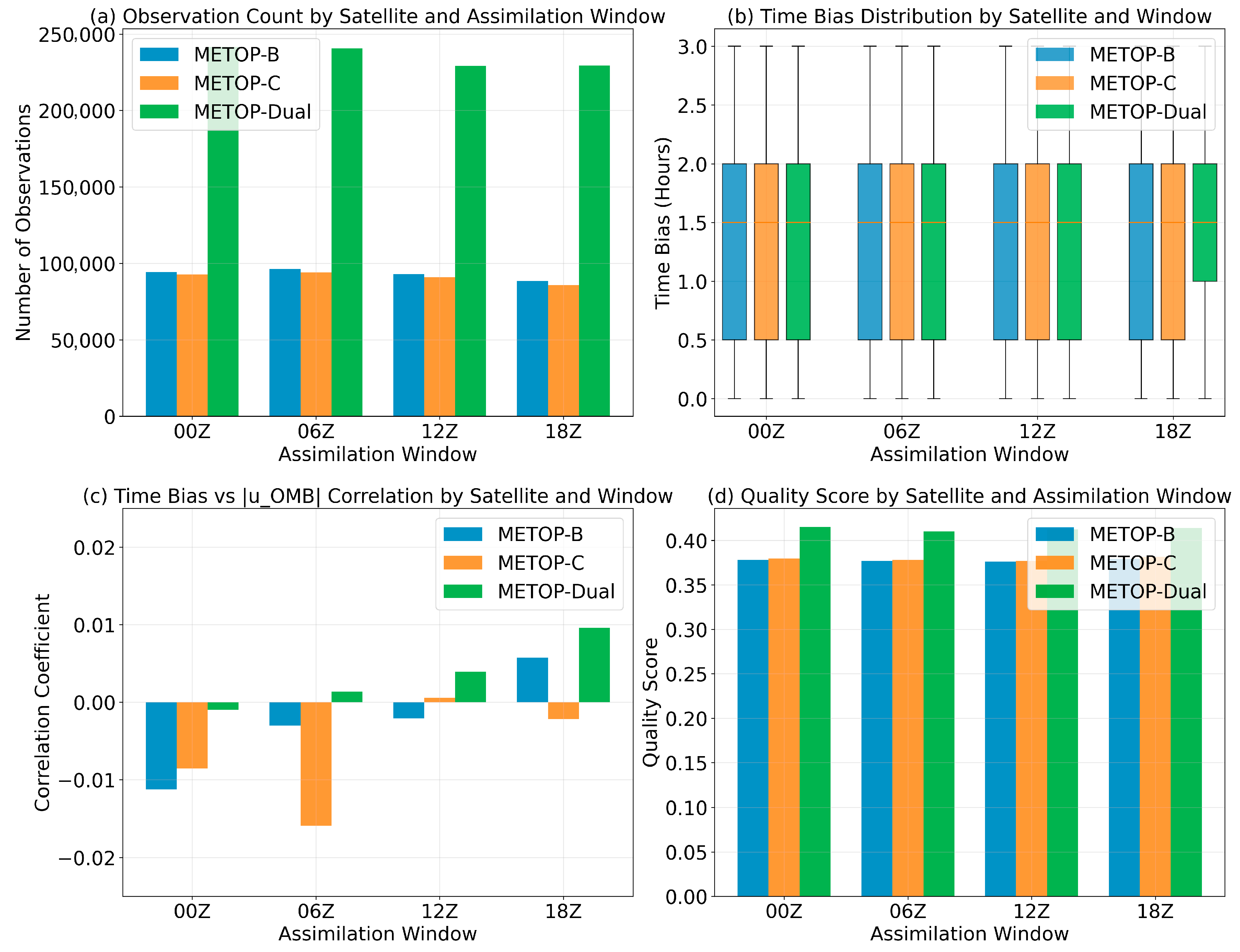
Figure 7 indicates all of the MetOp-B/C/Dual AMVs meet the temporal requirements for global data assimilation. MetOp-Dual provides approximately 2.5 times more observations than either MetOp-B or MetOp-C in each assimilation window, ensuring adequate data coverage (Figure 7a). The average time bias across all three AMVs during the four assimilation cycles (00Z, 06Z, 12Z, 18Z) ranges from 1.41 to 1.48 h (Figure 7b), falling within acceptable limits for operational assimilation systems.
To evaluate how the time differences among different satellites (MetOp-/B/C, MetOp-Dual) affect the assimilation, we carry out the correlation analysis between time bias and Observation-Background (O-B) for each of the three kinds of AMVs. (Note that the specific meaning and indication of Observation-Background will be given in Section 4.2.) Correlation analysis reveals consistently low coefficients (−0.016 to 0.010) between time bias and O-B (Figure 7c), suggesting the negligible influence of temporal differences on assimilation quality.
Furthermore, we define the Quality_Score of each satellite based on Equations (4)–(6) to enable comparison across different satellites and assimilation windows.
u_quality = 1/(1 + |u_OMB|)
v_quality = 1/(1 + |v_OMB|)
Quality_Score = (u_quality + v_quality)/2
where u_OMB is the mean O-B departures of u component and v_OMB is the mean O-B departures of v component. The assessment of Quality_Score further confirms the robustness of the observations, with O-B-based quality scores ranging from 0.376 to 0.415 and demonstrating consistent performance across different satellites and time windows. Notably, MetOp-Dual shows slightly better quality scores (0.410–0.415) compared to MetOp-B (0.376–0.379) and MetOp-C (0.377–0.381) (Figure 7d).
In conclusion, the MetOp satellite constellation provides temporally homogeneous and qualitatively stable AMV observations suitable for CMA-GFS.

4.2. Observation Space Verification

Observation space verification refers to the process of using the observation operator to transform the analysis variables into their observation equivalents. For directly observed data such as wind guidance, the observation operator primarily involves spatial interpolation. For remote sensing data like radiance, it also includes converting the model’s analysis variables into the observed physical quantities (e.g., top-of-atmosphere radiance at specific wavelengths). A fundamental principle is that a reduction in the Observation-minus-Background (O-B) departure, based on large-sample statistics, indicates that the analysis field has moved closer to the observations, signifying a positive assimilation effect. Conversely, an increase in O-B suggests a negative impact.
Table 1 presents the statistical results of the standard deviations of O-B for radiosonde, surface observations, aircraft reports, satellite radiance, and various sources of AMVs. From radiosonde, surface observation, aircraft, satellite radiance to AMV listed, the Sensitivity Experiment consistently shows smaller O-B std than the Control Experiment. This indicates the assimilation of MetOp series AMVs brings the model background closer to the observations.
In particular, the greatest improvement comes from the surface pressure, evidenced by the lowest O-B std ratio (0.9659). Unlike bright temperature or AMVs, which inherently contain uncertainties in inversion or retrieval, surface pressure provides a relatively more accurate and reliable benchmark for real atmospheric state. This further demonstrates the positive impact on model background of assimilation of MetOp series AMVs.
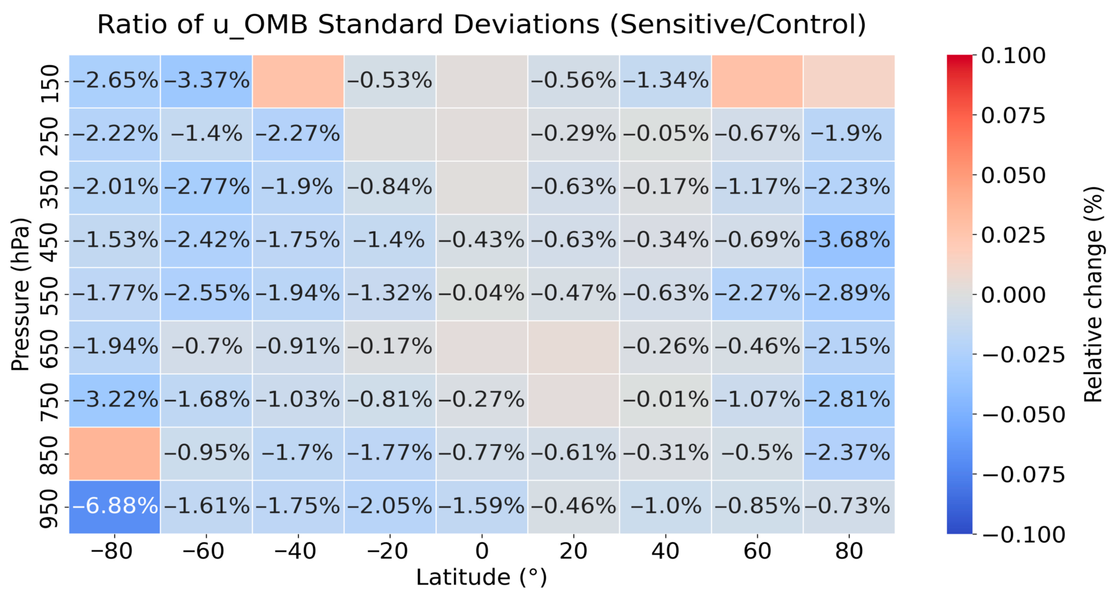
GOES16 and NOAA20 are the two representative satellites covering mid to low latitudes and high latitudes, respectively (Figure 1). In Table 1, the GOES16 series exhibits relatively small O-B std among the geostationary satellite AMVs, while NOAA20 shows relatively small O-B std in polar regions, reflecting the potentially high quality of GOES16 and NOAA20 AMVs. Therefore, GOES16 and NOAA20 were selected for further analysis. The reduction rate of the O-B std of the Sensitivity Experiment relative to the Control Experiment was defined as “a”, and the zonal–vertical distribution characteristics of “a” were statistically analyzed (Figure 8). The results reveal that “a” is negative across most latitudes and altitudes, indicating that in the majority of latitudinal zones and altitude ranges, the background field in the Sensitivity Experiment is closer to the observations than in the Control Experiment. Notably, the absolute values of “a” are larger in high-latitude regions than in low-latitude regions, suggesting that improvements are more pronounced in high latitudes—where MetOp series AMVs are predominantly distributed.
However, isolated positive “a” values were observed at 900–800 hPa in the Arctic, 200–100 hPa in the Antarctic, and in the middle and upper troposphere of the tropics, indicating that some localized negative effects exist. The largest positive value of a in 900–800 hPa over the Arctic appears more interesting as the nearby value of 1000–900 hPa exhibits the largest negative value of a. The reason for this “dipole contrast” may lie in the large gap in the proportion of MetOp series AMVs over the two layers in the Arctic, which is illustrated by Figure 6c. AMVs in the 1000–900 hPa in the Arctic are mostly from MetOp series, while their share is much less in the 900–800 hPa. Also, the vertical covariance of background field error in the Arctic, which is set in CMA-GFS, may inhibit the upward propagation of the “good signal” in 1000–900 hPa to the 900–800 hPa layer. The small positive or small negative a values in the middle-upper tropic atmosphere could also be largely attributed to the smaller ratio of MetOp series AMVs, which imposes weak impact on the background. Some positive a values in the upper troposphere may be attributed to the quality control scheme that forcefully discards the MetOp AMVs above 200 hPa.
In summary, the MetOp series AMVs generally bring the observation equivalents in the Sensitivity Experiment closer to actual observations compared to the Control Experiment, with this effect being particularly evident in mid to high latitudes.

4.3. Model Space Verification

In cyclic assimilation experiments, the analysis field generated by the model at a given time serves as the background field for the next time step. Both the analysis field and the background field are gridded. Evaluating the model’s gridded variables directly represents an alternative approach to background field verification independent from the observation space verification and is termed model space verification.
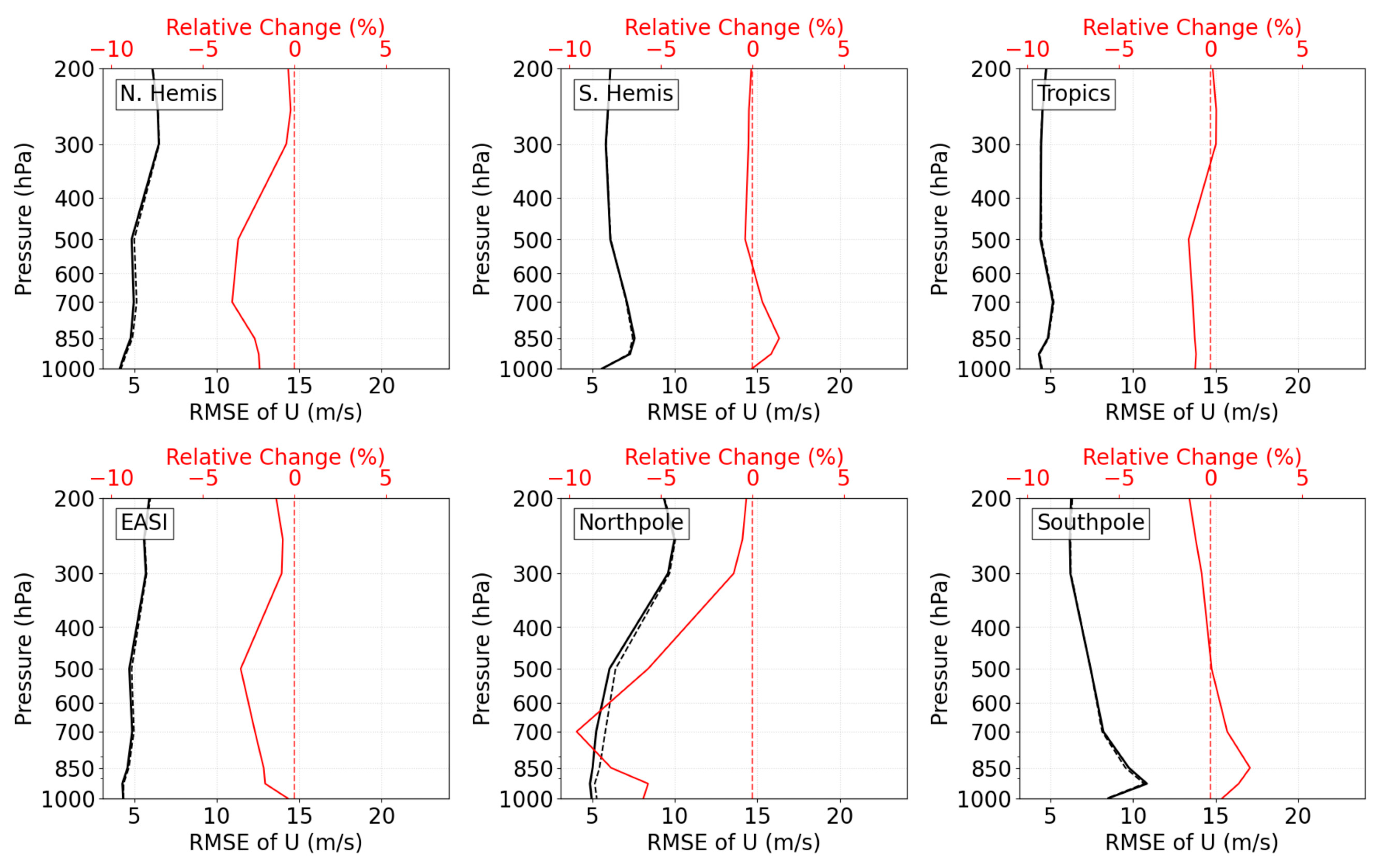
Using ERA5 reanalysis data as the benchmark, model space verification is conducted for the zonal wind component (u). The differences in u between each of the two experiments and ERA5 are analyzed to check the wind improvement. The results demonstrate that, across various regions—including the Northern Hemisphere (20°N–90°N, 0°–360°E), Southern Hemisphere (90°S–20°S, 0°–360°E), tropics (20°S–20°N, 0°–360°E), East Asia (15°N–65°N, 70°E–145°E), Arctic (70°N–90°N, 0°–360°E), and Antarctic (90°S–70°S, 0°–360°E)—the RMSE between the analysis fields of the Sensitivity Experiment and ERA5 is smaller than that between the Control Experiment and ERA5 (Figure 9). Notably, the reduction in RMSE is more pronounced in the middle troposphere than in the upper troposphere. The Arctic exhibits the greatest RMSE reduction among all regions, with an average decrease of 4.6% in the mid-atmosphere (500–700 hPa) (Figure 9), while the tropics exhibit the smallest improvement. This is reasonable because the tropics are already well-observed by geostationary AMVs, while the MetOp series provides relatively few AMVs in this region (exclusively from MetOp-Dual). Consequently, the incremental benefit of adding MetOp AMVs is smaller in the tropics.
For the South Pole and Southern Hemisphere, the middle–low troposphere exhibits positive performance while the upper exhibits negative or neutral. This may be attributed to two factors. First, the sparse conventional observations over the Southern Ocean and Antarctica create greater dependence on satellite data, making these regions more sensitive to biases in the AMV retrievals. Second, the complex quality control procedures for AMVs in data-sparse regions might inadvertently filter out valid observations or retain biased ones, particularly at upper levels where cloud-tracked winds face greater challenges in height assignment and wind derivation.
Generally, these findings indicate that the wind fields in the Sensitivity Experiment are closer to ERA5 compared to the Control Experiment, providing further evidence that the assimilation of MetOp series AMVs improves the CMA-GFS background wind fields.
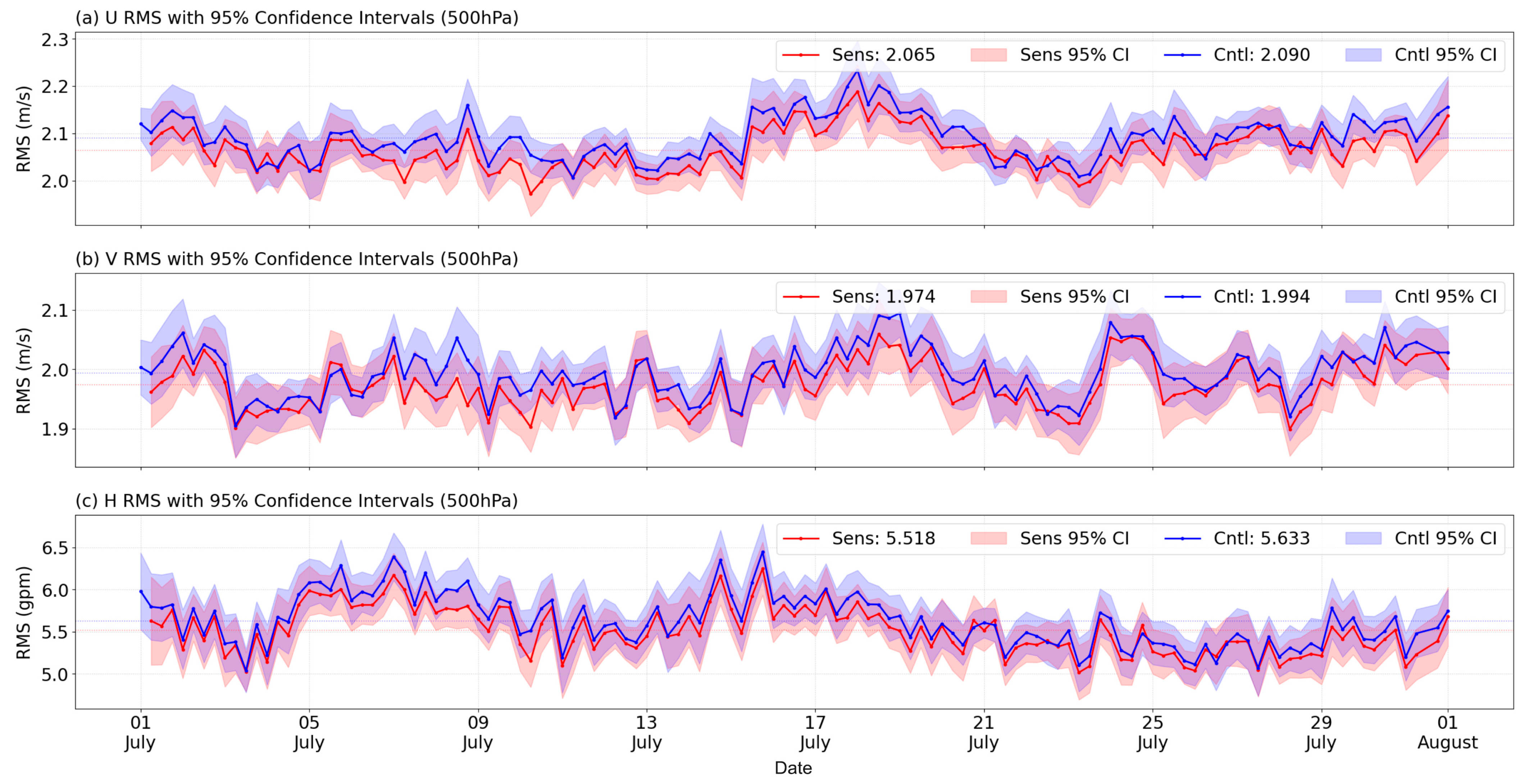
On a global scale, the assimilation of MetOp series AMVs leads to consistent reductions in root mean square error (RMSE) across key atmospheric variables at 500 hPa. The Sensitivity Experiment shows a zonal wind (U) RMSE of 2.065 m/s, compared to 2.090 m/s in the Control Experiment (Figure 10a). Similarly, the meridional wind (V) RMSE decreases from 1.994 m/s to 1.974 m/s (Figure 10b), and the geopotential height (H) RMSE improves from 5.663 gpm to 5.518 gpm (Figure 10c). Although the magnitude of these improvements is modest, the 95% confidence intervals of the Sensitivity Experiment remain consistently below those of the Control Experiment throughout the study period. This consistent separation indicates a positive effect of the method, suggesting that the RMSE reductions are unlikely to be attributable to sampling variability alone.
These results indicate that, after assimilating MetOp series AMVs, the global mid-tropospheric wind and height fields become closer to ERA5 reanalysis data. The persistent nature of these improvements suggests that MetOp AMVs provide a sustained positive impact on the CMA-GFS background field quality.

4.4. Forecast Result Analysis

The Anomaly Correlation Coefficient (ACC) quantifies the similarity in spatial patterns between forecast anomalies and observed anomalies, serving as a commonly used evaluation metric in meteorological forecasting to measure the resemblance between forecast fields and observational fields. Its core objective is to assess whether forecasts can accurately capture the anomalous distributions of weather systems.
The “usable forecast days” typically refers to the maximum forecast lead time during which forecast skill meets a predefined threshold (e.g., ACC ≥ 0.6). The number of days with ACC ≥ 0.6 for 500 hPa geopotential height fields is generally used to represent the usable forecast days. Based on both the contrast and Control Experiments, 10-day forecast experiments are conducted over a one-month period (from 1 July to 1 August 2024) as mentioned in Section 2.2. Evaluations of 500 hPa geopotential height fields revealed that the global usable forecast days in the Sensitivity Experiment are 8.37 days, exceeding the 8.15 days in the Control Experiment. This indicates that assimilating MetOp series AMV products improved the overall forecast performance of the CMA-GFS model.
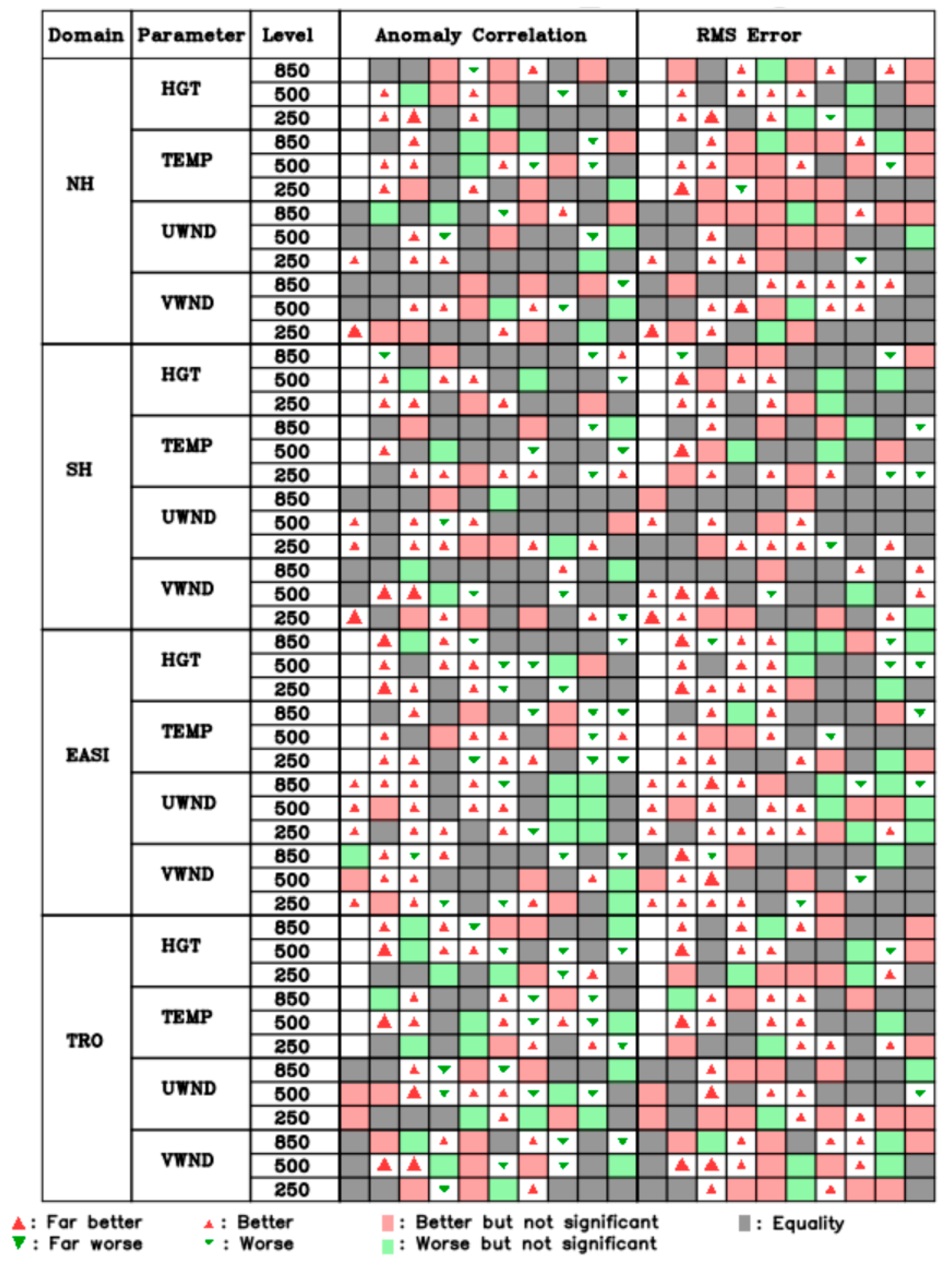
Further assessments are performed for forecasts of upper-level (250 hPa), mid-level (500 hPa), and lower-level (850 hPa) height fields, temperature fields, zonal winds, and meridional winds across the Northern Hemisphere, Southern Hemisphere, East Asia, and tropical regions, as shown in Figure 11. The results demonstrate that the Sensitivity Experiment generally outperformed the Control Experiment in terms of ACC (more red indicates better performance) and RMSE error reduction, with particularly notable improvements in short-range (0–3 day) forecasts (evidenced by more red triangles). Therefore, it can be concluded that the assimilation of MetOp series AMVs enhanced the overall forecast performance of the CMA-GFS model, particularly in the short-range forecasting.

5. Conclusions

This study developed assimilation techniques for MetOp series AMVs (including MetOp-B, MetOp-C, and MetOp-Dual) within the CMA-GFS system. Through one-month Control and Sensitivity experiments, the improvements in CMA-GFS background and forecast fields resulting from assimilating MetOp AMVs were evaluated. Key findings are as follows:
  • Quality Control and Thinning Processing Schemes: A quality control protocol is developed to retain MetOp AMVs with confidence levels exceeding 80%, altitudes below 200 hPa, and horizontal wind speeds under 30 m/s. Additionally, a three-dimensional thinning scheme was implemented with 200 km horizontal and 50 hPa vertical intervals. These measures increased CMA-GFS’s total AMV observations by 25%, with MetOp AMVs accounting for 41.1% of mid-tropospheric (500–600 hPa) AMV data and over 80% of AMV data in polar mid-levels. These preprocessing measures enhanced the utilization of MetOp AMVs and helped fill observational gaps, particularly in data-sparse regions like the polar areas and the mid-troposphere.
  • Background Field Improvements: Observation space and model space validations demonstrated that MetOp AMVs generally improved CMA-GFS’s global background fields by: (a) bringing observation equivalents closer to direct measurements (e.g., radiosondes, aircraft reports, and radiance data), and (b) producing a more stable and accurate analysis field that aligns closely with ERA5 reanalysis. These improvements are most pronounced in polar and mid- to high-latitude regions. Notably, standard deviations of 500–700 hPa zonal wind (U) relative to ERA5 in the Arctic decreased by up to 4.6% after assimilating MetOp AMVs.
  • Forecast Performance Enhancements: Forecast experiments revealed consistent improvements in CMA-GFS forecast fields, particularly for short-range (0–3 day) predictions across multiple variables. Anomaly Correlation Coefficient (ACC) analysis indicated a 0.22-day increase in the usable forecast days for global 500 hPa geopotential height fields.
This study filled the gap in terms of applying MetOp-B, MetOp-C, and MetOp-Dual AMVs within CMA-GFS. The results prove the positive impact of MetOp AMVs on both background and forecast of CMA-GFS. The 0.22-day extension in the effective forecast range of the 500 hPa geopotential height provides forecasters with a longer window of confidence for medium-range pattern forecasting. Furthermore, the enhanced accuracy in the short-range (0–3 days) forecasting directly strengthens the model’s capability in severe weather prediction and alerting.
However, this research suggests three areas for future improvement. First, increased O-B RMSE values in specific vertical layers and latitude bands indicate persistent background-observation discrepancies. Future work will employ advanced diagnostic tools such as Forecast Sensitivity Observation Impact (FSOI) to quantify the contribution of individual AMV datasets. This will enable the development of dynamic, flow-dependent data thinning strategies and superobbing schemes to optimize the synergy between MetOp and other AMV sources, thereby maximizing their collective impact while minimizing error propagation. Second, seasonal experiments are planned with winter-month analyses. This will complement the current summer results and provide a comprehensive assessment of year-round performance. Third, although ERA5 is a reliable representation of the true atmospheric state, it assimilates MetOp AMV data itself, which introduces a potential circular dependency in the verification. Future work will include validation against independent observations to strengthen confidence in the results.

Author Contributions

Conceptualization, J.M. and Y.L.; methodology, J.M. and Y.L.; software, J.M.; validation, J.M., Y.L. and X.W.; formal analysis, J.M.; investigation, J.M., Y.L. and X.W.; resources, Y.L.; data curation, J.M.; writing—original draft preparation, J.M.; writing—review and editing, Y.L. and X.W.; visualization, J.M.; supervision, Y.L.; project administration, Y.L.; funding acquisition, J.M. and Y.L. All authors have read and agreed to the published version of the manuscript.

Funding

This research was supported by the National Natural Science Foundation of China (Grant No. U24A20605), Youth Fund of the CMA Earth System Modeling and Prediction Centre (Grant No. 582128) and the Innovation and Development Program of the China Meteorological Administration (CXFZ2025J093).

Data Availability Statement

ERA5 reanalysis dataset can be downloaded at https://cds.climate.copernicus.eu/datasets/reanalysis-era5-pressure-levels?tab=download (accessed on 1 April 2025) and MetOp dataset can be downloaded at https://navigator.eumetsat.int/product/EO:EUM:DAT:METOP:AVHAMV2D?query=AVHRR%20Atmospheric%20Motion%20Vectors%20(BUFR)%20-%20Metop%20-%20Global&s=advanced (accessed on 1 August 2025).

Acknowledgments

We thank Bin Zhao for providing the Getpy toolbox for postprocessing the forecast output of the CMA-GFS, and express our gratitude to Minyan Wang, Chuanwen Wei, Hongyi Xiao, Fu Wang and Hao Hu for their valuable suggestions and assistance in data processing and visualization.

Conflicts of Interest

The authors declare no conflicts of interest.

References

  1. Velden, C.S.; Hayden, C.M.; Nieman, S.J.W.; Paul Menzel, W.; Wanzong, S.; Goerss, J.S. Upper-tropospheric winds derived from geostationary satellite water vapor observations. Bull. Am. Meteorol. Soc. 1997, 78, 173–195. [Google Scholar] [CrossRef]
  2. Tomassini, M.; Kelly, G.; Saunders, R. Use and impact of satellite atmospheric motion winds on ECMWF analyses and forecasts. Mon. Weather. Rev. 1999, 127, 971–986. [Google Scholar] [CrossRef]
  3. Forsythe, M. Atmospheric motion vectors: Past, present and future. In Proceedings of the ECMWF Annual Seminar, Exeter, UK, 4–8 September 2007; pp. 1–79. [Google Scholar]
  4. Berger, H.; Langland, R.; Velden, C.S.; Reynolds, C.A.; Pauley, P.M. Impact of enhancedsatellite-derived atmospheric motion vector observations on numerical tropical cyclone track forecasts in the western north Pacific dur-ing TPARC/TCS-08. J. Appl. Meteorol. Climatol. 2011, 50, 2309–2318. [Google Scholar] [CrossRef]
  5. Zhou, R.D.; Xia, P.; Zhang, X.H.; Xu, N.; Min, M. Research progress and prospects of atmospheric motion vector based on meteorological satellite images. Rev. Geophys. Planet. Phys. 2024, 55, 184–194. (In Chinese) [Google Scholar] [CrossRef]
  6. Li, J.; Santek, D.; Li, Z.; Lim, A.; Di, D.; Min, M.; Velden, C.; Menzel, W.P. Tracking Atmospheric Motions for Obtaining Wind Estimates Using Satellite Observations—From 2D to 3D. Bull. Amer. Meteor. Soc. 2025, 106, E344–E363. [Google Scholar] [CrossRef]
  7. Eyre, J.R.; English, S.J.; Forsythe, M. Assimilation of satellite data in numerical weather prediction. Part I: The early years. Q. J. R. Meteorol. Soc. 2020, 146, 49–68. [Google Scholar] [CrossRef]
  8. Holmlund, K. The atmospheric motion vector retrieval scheme for meteosat second generation. In Proceedings of the Fifth Internationial Winds Workshop, Lorne, Australia, 28 February–3 March 2000; pp. 201–208. [Google Scholar]
  9. Zhao, J.; Gao, J.; Jones, T.A.; Hu, J. Impact of assimilating high-resolution atmospheric motion vectors on convective scale short-term forecasts: 2. Assimilation experiments of GOES-16 satellite derived winds. J. Adv. Model. Earth Syst. 2021, 13, e2021MS002486. [Google Scholar] [CrossRef]
  10. Kim, D.H.; Kim, H.M. Effect of assimilating Himawari-8 atmospheric motion vectors on forecast errors over East Asia. J. Atmos. Ocean. Technol. 2018, 35, 1737–1752. [Google Scholar] [CrossRef]
  11. Chen, Y.; Shen, J.; Fan, S.; Meng, D.; Wang, C. Characteristics of Fengyun-4A satellite atmospheric motion vectors and their impacts on data assimilation. Adv. Atmos. Sci. 2020, 37, 1222–1238. [Google Scholar] [CrossRef]
  12. Hautecoeur, O.; Borde, R. Derivation of wind vectors from AVHRR/MetOp at EUMETSAT. J. Atmos. Ocean. Technol. 2017, 34, 1645–1659. [Google Scholar] [CrossRef]
  13. ECMWF Assimilation Observation Monitoring Website. Available online: https://charts.ecmwf.int/catalogue/packages/obstat/?facets=%7B%22Parameter%22%3A%5B%5D%2C%22Data%20type%22%3A%5B%22Atmospheric%20Motion%20Vectors%22%5D%2C%22Category%22%3A%5B%22Satellite%20Data%22%5D%2C%22Instrument%22%3A%5B%22METOP-B%22%2C%22METOP-C%22%2C%22DUAL_METOP%22%5D%7D (accessed on 21 August 2025).
  14. AMV Activities and Progress at the Meteorological Service of Canada. Available online: https://cgms-info.org/html/iww14/talks/06_Posters/IWW14_Laroche_Poster.pdf (accessed on 21 August 2025).
  15. Upgrades of Polar AMVs Use in JMA’s Global NWP System. Available online: https://www.ssec.wisc.edu/meetings/iwwg/2023-meeting/presentations/upgrades-of-polar-amvs-use-in-jmas-global-nwp-system/ (accessed on 21 August 2025).
  16. Xiong, X.; Che, N.; Barnes, W. Terra MODIS on-orbit spatial characterization and performance. IEEE Trans. Geosci. Remote Sens. 2005, 43, 355–365. [Google Scholar] [CrossRef]
  17. NWP SAF AMV Monitoring: The 10th Analysis Report (AR10). Available online: https://cgms-info.org/wp-content/uploads/2024/08/nwpsaf_mo_tr_042.pdf (accessed on 21 August 2025).
  18. Daily SATOB Monitoring of METEO FRANCE. Available online: http://www.meteo.fr/special/minisites/monitoring/SATELLITE/SATOB/satob.html (accessed on 21 August 2025).
  19. Xue, J.; Zhuang, S.; Zhu, G.; Zhang, H.; Liu, Z.; Liu, Y.; Zhuang, Z. Scientific design and preliminary results of three-dimensional variational data assimilation system of GRAPES. Chin. Sci. Bull. 2008, 53, 3446–3457. [Google Scholar] [CrossRef]
  20. Yan, L.; Jishan, X.; Lin, Z.; Huijuan, L. Verification and Diagnostics for Data Assimilation System of Global GRAPES. J. Appl. Meteorol. Sci. 2016, 27, 1–15. [Google Scholar]
  21. Han, W.; Xue, J.S.; Xu, J.M.; Zhang, Q.S. Assimilation of FY2C AMV in GRAPES. In Proceedings of the Eighth International Winds Workshop, Beijing, China, 24–28 April 2006; EUMETSAT: Beijing, China, 2006; pp. 24–28. [Google Scholar]
  22. Wan, X.M.; Tian, W.H.; Han, W.; Wang, R.W.; Zhang, Q.S.; Zhang, X.H. The evaluation of FY-2E reprocessed IR AMVs in GRAPES. Meteorol. Mon. 2017, 43, 1–10. (In Chinese) [Google Scholar]
  23. Wan, X.; Gong, J.; Han, W. The Evaluation of FY-4A AMVs in GRAPES_RAFS. Meteorol. Mon. 2019, 45, 458–468. [Google Scholar] [CrossRef]
  24. Wan, X.; Han, W.; Tian, W.; He, X. The application of intensive FY-2G AMVs in GRAPES_RAFS. Plateau Meteorol. 2018, 37, 1083–1093. (In Chinese) [Google Scholar]
  25. Shen, X.; Su, Y.; Hu, J.; Wang, J.; Sun, J.; Xue, J.; Han, W.; Zhang, H.; Lu, H.; Zhang, H. Development and operation transformation of GRAPES globalmiddle-range forecast system. J. Appl. Meteorol. Sci. 2017, 28, 1–10. (In Chinese) [Google Scholar]
  26. Shen, X.S.; Wang, J.J.; Li, Z.C.; Chen, D.H.; Gong, J.D. China’s independent and innovative development of numerical weather prediction. Acta Meteorol. Sin. 2020, 78, 451–476. [Google Scholar]
  27. Zhang, W.; Shen, X.; Cao, X.; Sun, J.; Wu, J.; Peng, J.; Song, J.; Zhu, X.; Wang, J.; Zhang, Z. 70 years of development in China’s operational numerical weather prediction. Acta Meteorol. Sin. 2025, 83, 435–463. [Google Scholar] [CrossRef]
  28. Bormann, N.; Saarinen, S.; Kelly, G.; Thépaut, J.-N. The Spatial Structure of Observation Errors in Atmospheric Motion Vectors from Geostationary Satellite Data. Mon. Weather. Rev. 2003, 131, 706–718. [Google Scholar] [CrossRef]
  29. Zhou, L.; Divakarla, M.; Liu, X.; Layns, A.; Goldberg, M. An overview of the science performances and calibration/validation of joint polar satellite system operational products. Remote Sens. 2019, 11, 698. [Google Scholar] [CrossRef]
  30. Hersbach, H.; Bell, B.; Berrisford, P.; Hirahara, S.; Horányi, A.; Muñoz-Sabater, J.; Nicolas, J.; Peubey, C.; Radu, R.; Schepers, D.; et al. The ERA5 global reanalysis. Q. J. R. Meteorol. Soc. 2020, 146, 1999–2049. [Google Scholar] [CrossRef]
  31. Zhang, J.; Sun, J.; Shen, X.; Su, Y.; Ma, Z.; Jing, H.; Liu, Q.; Zhang, H.; Jiang, Q.; Chen, F. Key model technologies of CMA-GFS V4.0 and application to operational forecast. J. Appl. Meteorol. Sci. 2023, 34, 513–526. [Google Scholar] [CrossRef]
  32. Zhu, G. Interpretation of Several Basic Aspects of Atmospheric Data Assimilation. Meteorol. Mon. 2015, 41, 997–1006. (In Chinese) [Google Scholar] [CrossRef]
  33. Warrick, F.; Lean, K. Wind information from Satellites: Atmospheric Motion Vectors Passive Tracing with GEO Radiances; ECMWF: Barbour, AL, USA, 2025. [Google Scholar]
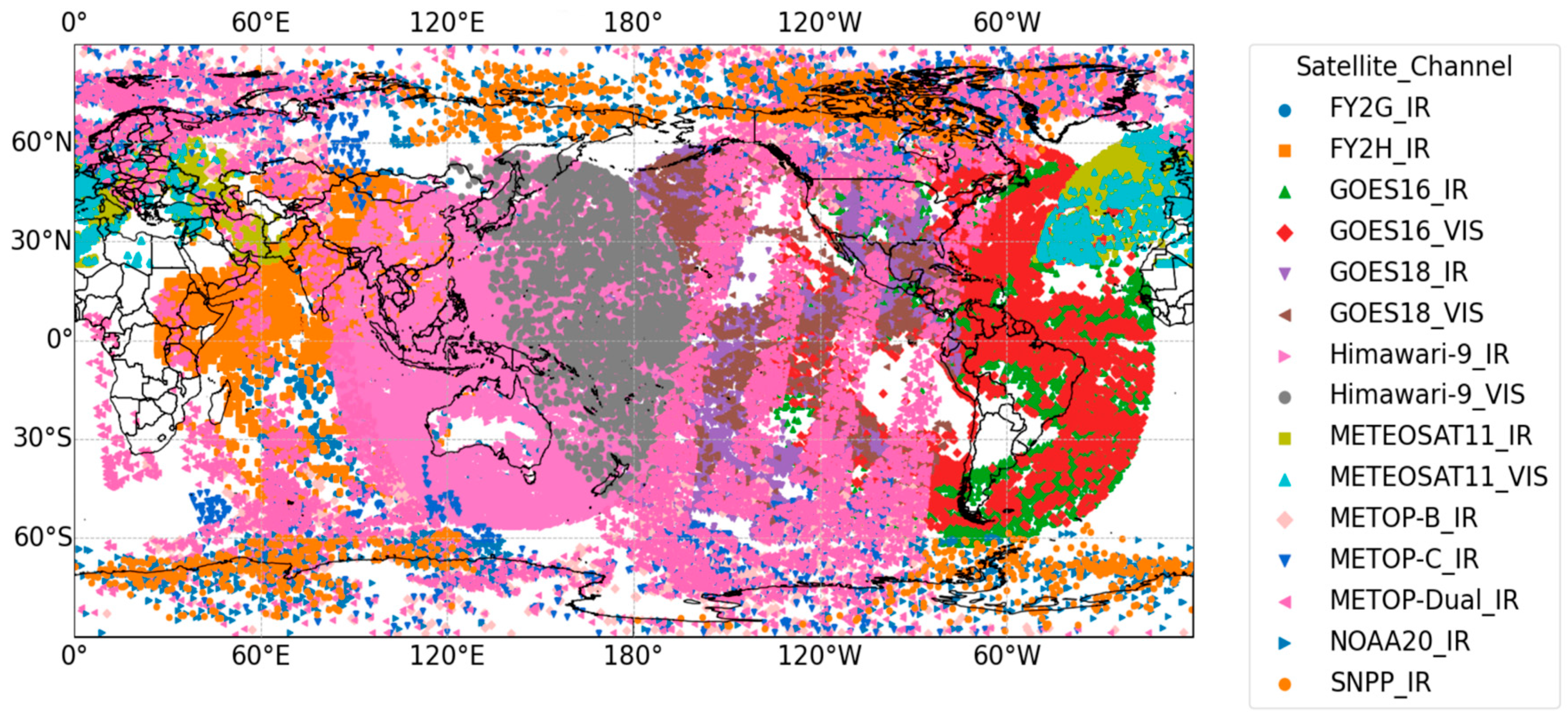
Figure 1. Distribution of AMVs in the CMA-GFS from 15:00 to 21:00 UTC on 1 July 2024 (IR: Infrared, VIS: Visible).
Remotesensing 17 03519 g001
Figure 2. Joint density distribution of MetOp-Dual observations and ERA5 horizontal wind speeds (Comparison Period: 18 February to 1 April 2023).
Remotesensing 17 03519 g002
Figure 3. Number of MetOp-Dual AMVs and the bias and RMSE of horizontal wind speeds relative to ERA5 by pressure levels. The red line denotes the 200 hPa level.
Remotesensing 17 03519 g003
Figure 4. Distribution of thinning anchors with ~200 km horizontal interval for AMV thinning.
Remotesensing 17 03519 g004
Figure 5. Comparison of two-dimensional thinning (a) and three-dimensional thinning (b) for the assimilation time slot of 02:45–03:15 UTC on 25 May 2024. The red stars denote the anchor points created in Step 1. The grey points denote the discarded observations by the thinning process. The other points of different colors denote the retained observations by the thinning process, with their pressure level in the right colorbar.
Remotesensing 17 03519 g005
Figure 6. Statistics on the number of AMVs in the Sensitivity Experiment from 1 July to 1 August 2024. (a) Percentages of all kinds of AMV observations; (b) vertical profiles of AMV observations, where IR: infrared; VIS: visible; (c) latitude–pressure ratios of MetOp series AMVs, with color shading indicating the proportion and black lines indicating the total number of all sources of AMV observations, corresponding to the right y-axis.
Remotesensing 17 03519 g006
Figure 7. Impact of each of the time difference among MetOp-B, MetOp-C, and MetOp-Dual AMVs on assimilation quality.
Remotesensing 17 03519 g007
Figure 8. Latitude–height distribution of the relative change rate of O-B standard deviation (std) of the Sensitivity Experiment compared to the Control Experiment, based on GOES16 and NOAA20, with negative values annotated.
Remotesensing 17 03519 g008
Figure 9. Vertical distribution of root mean square (RMSE) differences in zonal wind U relative to ERA5 across different regions. (Solid black lines represent the Sensitivity Experiment, dashed black lines represent the Control Experiment, corresponding to the bottom coordinate axis; solid red lines indicate the relative change rate of the Sensitivity Experiment relative to the Control Experiment, corresponding to the top coordinate axis.)
Remotesensing 17 03519 g009
Figure 10. Time series of RMSEs in mid-tropospheric (500 hPa) U (a), V (b), and geopotential height (H) (c) relative to ERA5 for the Sensitivity Experiment and Control Experiment.
Remotesensing 17 03519 g010
Figure 11. The forecast score card of the Sensitivity Experiment against Control Experiment, running at 1200 UTC everyday from 1 July to 1 August 2024. The first column in each card lists four regions: NH, Northern Hemisphere (20–90°N); SH, Southern Hemisphere (20–90°S); EASI, East Asia (20–55°N, 70–145°E); and TRO, tropics (20°S–20°N). The second column in each card lists the key atmospheric variables: HGT, geopotential height; TEMP, temperature; UWND, zonal wind; and VWND, meridional wind. Each variable in each region is separately evaluated at 850, 500, and 250 hPa. The remaining columns are divided into two parts (one for anomaly correlation and one for the RMSE), each of which consists of 10 columns for the 10 forecasting days. The color and shape show the significance, which is determined by the ratio of the score difference and confidence interval width (d/s). The large upward-pointing red triangles denote “far better” (d/s > 3); the small upward-pointing red triangles denote “better”(3 > d/s ≥ 1); the pink squares denote “better, but not significant”(1 > d/s ≥ 0.5); the large downward-pointing green triangles denote “far worse”(d/s < −3); the small downward-pointing green triangles denote “worse” (−1 ≥ d/s ≥ −3); the green squares denote “worse, but not significant” (−0.5 ≥ d/s >−1); and the gray squares denote “equality” (0.5 > d/s > −0.5).
Remotesensing 17 03519 g011
Table 1. Standard deviations (std) of Observation-Background (O-B) for various types of data and variables in the contrast experiment versus the Control Experiment (values in bold indicate ratios less than 1).
Data Type VariableO-B Std
Control ExperimentSensitivity ExperimentSensitivity/Control
RadiosondeU (m/s)2.7732.7570.9942
V (m/s)2.6872.6680.9929
Surface ObservationSurface Pressure (hPa)0.73660.71150.9659
Aircraft ReportU (m/s)2.33462.32360.9953
Tem (K)1.02581.02410.9983
NOAA20 ATMS
(Advanced Technology Microwave Sounder)
Brightness Temperature (K)0.78830.77430.9822
AMV
(Satellite_Channel, IR: Infrared, VIS: Visible)
GOES16_IR2.73462.7120.9917
GOES16_VIS1.94441.93020.9927
Himawari-9_IR2.43732.41360.9903
Himawari-9_VIS2.14342.1260.9919
METEOSAT11_IR3.87443.86360.9972
METEOSAT11_VIS2.15722.15450.9987
NOAA20_IR3.23113.15380.9761
SNPP_IR3.25713.19070.9796
Disclaimer/Publisher’s Note: The statements, opinions and data contained in all publications are solely those of the individual author(s) and contributor(s) and not of MDPI and/or the editor(s). MDPI and/or the editor(s) disclaim responsibility for any injury to people or property resulting from any ideas, methods, instructions or products referred to in the content.