Highlights
What are the main findings?
- Machine learning regression, integrating both authoritative and crowdsourced data, generated 20 m resolution air temperature maps for Milan during heatwaves, with higher accuracy observed during late afternoons and nights.
- Hyperspectral data was successfully applied to evaluate how the abundance of surface materials influences air temperature, indicating warming and cooling responses among materials
What is the implication of the main finding?
- The high-resolution maps capture intra-urban temperature variability, including a pronounced urban heat island (UHI) effect, with central areas up to 3–5 °C warmer and urban parks providing a cooling effect of 1–2 °C.
- These results provide important data to support urban heat risk assessment, model validation, and the development of heat mitigation strategies for cities facing extreme heat.
Abstract
High-resolution air temperature (AT) data is essential for understanding urban heat dynamics, particularly in urban areas characterised by complex microclimates. However, AT is rarely available in such detail, emphasising the need for its modelling. This study employs a Random Forest regression framework to predict 20 m resolution AT maps across Milan, Italy, for 2022. We focus on seasonal heatwave periods, identified from a long-term climate reanalysis dataset, and multiple diurnal and nocturnal phases that reflect the daily evolution of AT. We predict AT from a high-quality dataset of 97 authoritative and crowdsourced stations, incorporating predictors derived from geospatial and Earth Observation data, including Sentinel-2 indices and urban morphology metrics. Model performance is highest during the late afternoon and nighttime, with an average between 0.33 and 0.37, and an RMSE between 0.7 and 1.4 °C. This indicates modest, yet reasonable agreement with observations, given the challenges of high-resolution AT mapping. Daytime predictions prove more challenging, as noted in previous studies using similar methods. Furthermore, we explore the potential of hyperspectral (HS) data to estimate surface material abundances through spectral unmixing and assess their influence on AT. Results highlight the added value of HS-derived material abundance maps for insights into urban thermal properties and their relationship with AT patterns. The produced maps are useful for identifying intra-urban AT variability during extreme heat conditions and can support numerical model validation and city-scale heat mitigation planning.
1. Introduction
1.1. Background and Motivation
The latest European climate risk assessment identifies drought and extreme heat as some of the highest risks Europe faces under future climate change [1]. Without sustained intervention, increasing heat exposure will reduce liveability, productivity, and equity in urban areas, which are more affected than the surrounding natural environments due to the urban heat island (UHI) effect [2,3,4]. Within the global warming trend, the Mediterranean region, including Italy, has been identified as a climate change hotspot [5], with temperatures projected to rise about 20% faster than the global mean and rainfall decreasing, making its societies and ecosystems highly vulnerable [6].
Heat stress is particularly pronounced during episodes of extreme heat conditions, known as heatwave (HW) events [7]. For this reason, the increasing frequency and intensity of HWs induced by climate change represent a threat to human well-being, significantly contributing to the rise of heat-related mortality, especially among vulnerable populations such as the elderly [8,9]. For instance, the extreme heatwaves of 2022 have been associated with 60,000 to 70,000 excess deaths in Europe [10].
UHI is a general term that describes the temperature difference between urban and surrounding rural areas [3]. Within this phenomenon, two main types are commonly distinguished: the surface UHI (SUHI), derived from land surface temperature (LST) as captured by thermal satellite data, and the canopy-layer UHI (CUHI), which reflects variations in near-surface air temperature (AT). Owing to their wide availability, thermal satellite data are commonly used to assess urban heat risk by monitoring SUHI [11,12]. But, as highlighted by [13], this approach should be applied with caution as heat stress is driven by AT and not necessarily LST. In this context, AT is among the most critical variables, alongside apparent temperature and humidity, for assessing CUHI and characterising the thermal conditions experienced by the population [13,14,15]. Furthermore, AT and CUHI exhibit diurnal and seasonal trends [16,17], while varying significantly across space according to urban morphological features and land cover [3,18]. Therefore, the availability of gridded, high-resolution AT temporal data is essential for monitoring the spatial and temporal patterns of thermal discomfort and CUHI. However, unlike LST, it is difficult to obtain spatially continuous AT measurements. Multiple issues arise related to the availability, resolution, and quality of this kind of data, as detailed in the following two subsections.
1.2. AT Monitoring and Estimation
AT is observed by meteorological stations belonging to both official and crowdsourced sensor networks. Official weather stations typically provide high-quality data compliant with the World Meteorological Organisation standards [19]. However, due to the high installation and maintenance costs of professional stations, the spatial density of official weather networks is usually quite limited [20].
For this reason, there is increasing interest in crowdsourcing, using citizen weather stations (CWSs) to collect meteorological data for detailed, cost-efficient microclimate monitoring [21,22,23]. However, these measurements often lack quality standard verification and can be affected by a non-optimal sensor placement, thus demanding preliminary data cleaning [24,25]. Besides CWSs, crowdsourced data can be obtained through mobile measurements using portable sensors, which allow for the collection of AT transects [26,27,28,29].
While weather stations provide point-based measurements, some gridded AT data with continuous spatial coverage are available, coming from climate reanalysis products. They combine observations with numerical weather prediction models to reconstruct past atmospheric conditions. Notable examples include ERA5 (31 km) [30], ERA5-Land (9 km) [31], and UERRA for Europe (5.5 km) [32], with higher-resolution datasets available for some countries, such as for Germany (1 km) [33], France (8 km) [34], and Italy (2.2 km) [35]. While useful for large-scale and long-term analyses, their coarse resolution limits their ability to capture urban microclimate variability and thus a high-resolution assessment of AT patterns within cities.
1.3. AT Modelling Techniques and State of the Art on Regression-Based Methods
In order to generate continuous maps of AT, multiple approaches have been proposed and exploited in the literature. The methodology is chosen taking into account multiple aspects, e.g., the spatial scale, data availability, computational resources, and application scope. Essentially, a broad distinction can be made between numerical microclimate models and data-driven statistical techniques. The former are based on the modelling of atmospheric processes and physical parameterisation of atmospheric components at the urban scale, thus producing gridded AT predictions by solving physics-based equations. Several models have been developed, providing datasets with different levels of detail, such as WRF-Urban [36], PALM [37], UrbClim [38], and COSMO-CLM [39], among others.
On the other hand, data-driven statistical techniques aim to predict AT at locations without available measurements. The simplest methods in this category are spatial interpolation techniques, such as inverse distance weighting and kriging [40,41,42]. They assume that the phenomenon has a strong spatial dependence and rely on the principle of spatial autocorrelation. They are effective over small areas with dense station coverage, but are limited in capturing the effects of land use, topography, or surface materials that strongly influence AT variability in heterogeneous urban landscapes. To overcome these limitations, regression-based methods are often used. They include techniques to train statistical models that provide a function between AT and a set of predictors available with spatial continuity across the study area. Some examples of classic regression techniques include multiple linear regression, land use regression, and geographically weighted regression (GWR) [43,44,45,46]. While methods such as GWR address spatial heterogeneity, they still rely on linear assumptions that may limit their performance in complex urban contexts.
Machine learning (ML) and deep learning (DL) techniques offer a more flexible alternative. These models can handle nonlinearities, multicollinearity, and interactions that are difficult or impossible to model using the classic approaches mentioned above. They require large quantities of data to learn from; therefore, Earth Observation (EO) data is often incorporated due to its spatial coverage and temporal frequency, as demonstrated in previous studies [40,45,47,48,49,50,51,52].
In the context of Italy, several studies have applied AT modelling techniques, including co-kriging [41], although most have relied on regression-based approaches [53,54,55,56]. However, these efforts often produced coarse-resolution outputs, typically at 1 km. This highlights the need for high-resolution AT prediction, which will be addressed in this study.
1.4. Research Objectives and Paper Structure
Considering the gap in the high-resolution AT mapping summarised in the previous section, the objectives of the present research can be outlined as follows:
- To map the diurnal and seasonal evolution of AT during HWs in Milan using a data-driven ML regression model trained on crowdsourced AT measurements and geospatial and EO predictors, producing spatially continuous high-resolution maps that capture AT dynamics. To the best of our knowledge, no fine-scale AT mapping using regression-based methods has been conducted previously for this study area;
- To evaluate the potential of hyperspectral (HS) satellite imagery for understanding the influence of surface material abundances on AT; this aspect represents a novelty in the literature.
2. Materials and Methods
2.1. Study Site
This study focuses on the greater metropolitan area of the city of Milan, located in northern Italy, which spans approximately 80 km by 60 km as shown in Figure 1. It lies primarily within the Lombardy region, with a small portion extending into the Piedmont region. According to the Köppen–Geiger climate classification, Milan belongs to a humid subtropical climate (Cfa), also known as a warm-temperate climate [57,58]. It features hot, humid summers, as well as cool to mild winters. Milan’s metropolitan area is the second-largest urban agglomeration in Italy, after Rome, with a population exceeding 3 million [59]. The topography is predominantly flat, with most areas below 200 m.a.s.l. and an average elevation of 141 m. To the north, the elevation gradually increases, finally reaching a hilly area where the highest hills reach elevations between 500 and 600 m.
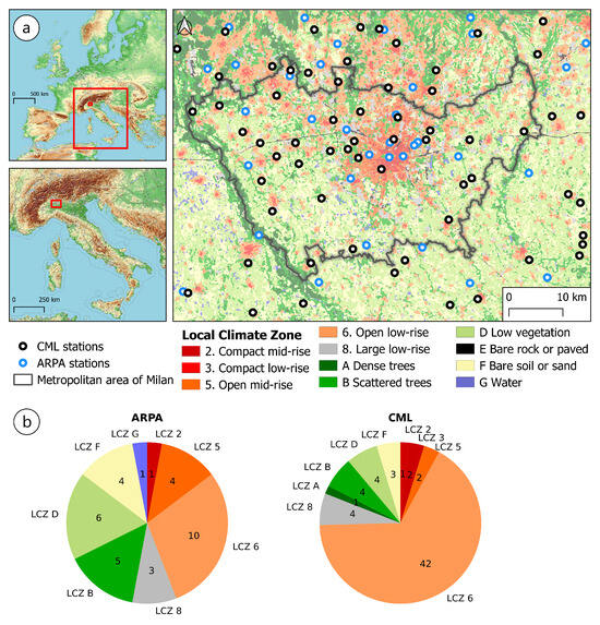
Figure 1.
Study area in Milan, Italy. (a) Distribution of authoritative ARPA and crowdsourced CML meteorological stations overlaid on the LCZ map for June 2022; basemap: OpenTopoMap (opentopomap.org/, accessed on 22 July 2025); (b) pie chart showing the number of ARPA and CML stations assigned to each LCZ class based on the dominant class within a 75 m circular buffer.
The city is located within the highly urbanised Po River Valley, a wide and low-lying basin surrounded by the Alps to the north and west. This geographical setting is crucial for the urban climate of Milan as it restricts airflow and causes heat to accumulate, thus reducing the potential for wind-driven cooling [3]. Consequently, this leads to the strengthening of the CUHI effect, especially during the summer months.
In addition, in 2022, the focus year of this study, the area experienced a severe meteorological drought [60]. The event led to a scarcity of precipitation that affected a large part of Europe, with Northern Italy among the most impacted regions. This is relevant to the present analysis, as decreased rainfall and low soil moisture content are known to reduce CUHI [61]. Due to suppressed evapotranspiration, the cooling effect of vegetation is reduced, resulting in a smaller AT difference between vegetated and urban areas.
2.2. Weather Station Data
Interpolation of AT requires a dense, reliable and spatially continuous network of well-distributed meteorological stations in the study area [40,48,49]. One major drawback of this approach is that such networks are rarely available unless specifically deployed for research, as in several European cities [44,62,63,64,65]. Often, they are used directly from crowdsourced platforms such as Netatmo [66]. In the case of the Lombardy region, an established crowdsourced sensor network is already in place. Therefore, this study builds on the existing crowdsourced sensor infrastructure and integrates it with an authoritative network, resulting in a combined dataset of 97 stations active during 2022. Spatial distribution of both networks is reported in Figure 1, along with the majority LCZ class.
Authoritative temperature data were obtained from the Regional Environmental Protection Agency (Agenzia Regionale per la Protezione dell’Ambiente, https://www.arpalombardia.it/, accessed on 24 April 2025), which operates 34 stations in the study area, providing measurements at 10 min intervals. To enhance spatial coverage, data from the Centro Meteorologico Lombardo (CML) amateur network were integrated (http://www.centrometeolombardo.com/, accessed on 24 April 2025). CML is a volunteer-based association focused on meteorology, operating a dense network of AT sensors distributed throughout the study area. For this study, they provided complete 2022 AT records for 63 stations which use the same sensor model (Davis Vantage Pro 2), ensuring consistency and comparability throughout the network [67]. Three stations record at 1 min intervals, and the remaining 60 at 5 min intervals.
Although crowdsourced data offer valuable microclimatic detail, they require rigorous quality control due to potential sensor misplacement (e.g., proximity to walls) [21,24,68]. For this reason, CML data were cleaned using ARPA as a reference, given its reliable, quality-controlled ground measurements. A virtual ARPA station was created by aggregating observations of all stations at each time step into a mean and standard deviation (SD). Although ARPA is highly reliable, z-score outlier removal was applied to remove minor inconsistencies (<0.01% observations removed). The CML cleaning procedure is partially based on [69] and includes three steps, outlined in Figure 2. After removing climatologically unlikely values in step (i), ARPA is used in the following two cleaning steps, step (ii) and (iii), aiming to filter out local outliers from the CML time series. During the cleaning process, all CML data were resampled to 10 min intervals to align with ARPA.
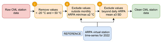
Figure 2.
Flowchart illustrating the quality control pre-processing steps applied to CML data.
The cleaning statistics per CML station are shown in Figure 3. Step (i) resulted in the removal of only 36 observations, while step (ii) excluded an additional 2287. Together with step (iii), which removed 8789 observations, the total number of removed observations amounted to 11,112. Given that the full dataset consists of 3,311,280 records across 63 stations at a 10 min resolution, this represents less than 0.4% of all CML observations, indicating a strong agreement with ARPA. Only five stations had more than 1% of observations removed, with a maximum of 6.5%.
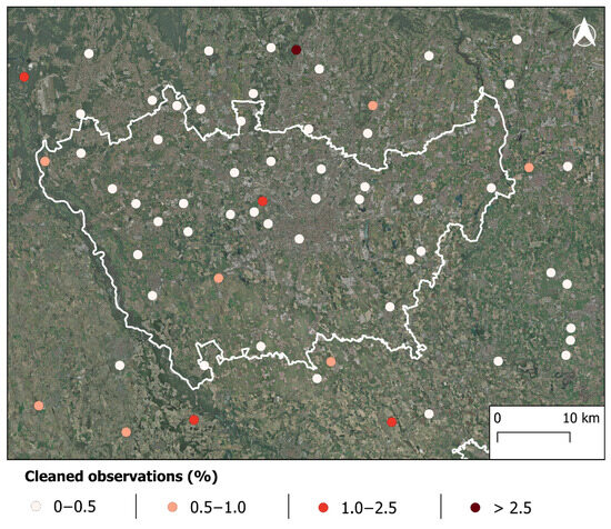
Figure 3.
Percentage of removed observations per CML station.
As shown in Figure 4, CML’s annual daily temperature cycle shows a close match to ARPA, with temperatures strongly correlated ( = 0.99). For most of the year, ARPA tends to be slightly warmer than CML, typically within 0.2 °C. During summer, such a difference is slightly enhanced, reaching up to 0.6 °C. Given that CML sensors have a stated accuracy of ±0.3 °C, these differences are within a reasonable margin [67]. An annual root mean squared error (RMSE) of 0.27 °C further confirms the reliability of CML data and supports its use in this study.
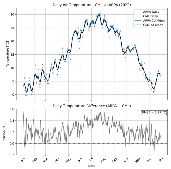
Figure 4.
Annual daily temperature cycle (top) and daily temperature differences (bottom) for ARPA and CML, based on the quality-controlled hourly dataset. In the upper panel, dots represent daily mean temperatures, while solid lines indicate the centred 7-day moving average.
After quality control, AT data were adjusted for elevation differences using a standard atmospheric lapse rate of °C/ as described in [24,25]. Observations were adjusted to a common reference elevation and set to the city’s mean elevation of 141 m. Sensor height and building height, in the case of a sensor placed on the rooftop, were incorporated into the correction. In total, fewer than 15 sensors are located on the rooftops.
2.3. HW Estimation and Selection
This study focuses on predicting AT during extreme heat conditions, i.e., HW periods, across different seasons in 2022. Consequently, it was necessary to select an HW detection method that would capture relevant events. Different methods have been proposed to identify and characterise HWs; however, no universal definition exists [70,71]. Depending on the purpose of the study and the region under analysis, various criteria may be applied, commonly including a minimum duration and intensity, that is, an average threshold exceedance. In the present study, HWs are defined following the approach of [72], which has also been applied in previous research [73,74]. Hence, an HW is defined as a period of at least three consecutive days where the daily maximum temperature exceeds the 90th percentile of long-term daily maxima, calculated using a centred 15-day moving window.
Rather than relying solely on point-based meteorological stations, this study utilises the VHR-REA_IT (Very High-Resolution dynamical downscaling of ERA5 Reanalysis over Italy) dataset to estimate HWs [35]. Developed by the Euro-Mediterranean Center on Climate Change (Centro Euro-Mediterraneo sui Cambiamenti Climatici, CMCC), VHR-REA_IT is produced through dynamical downscaling of the ERA5 reanalysis [30] over the Italian territory using the COSMO-CLM regional climate model [75]. It provides hourly data at approximately 2.2 km spatial resolution for the period of 1981–2023. The model includes the TERRA-URB module, which enhances the representation of urban land use and land–atmosphere interactions, making the dataset particularly suitable for urban climate assessments [76]. However, VHR-REA_IT is still subject to certain limitations and concerns, such as structural biases. For instance, refs. [77,78] demonstrated that models exhibit a warm summer bias of up to 3 °C in flat terrains such as the Po Valley and reduced performance in coastal regions.
The HW estimation method by [72] was applied to VHR-REA_IT. Long-term thresholds were calculated from the 1981–2021 reference period per grid cell, and threshold exceedance was calculated for each day in 2022. To ensure consistency across the area, a day was counted as HW only if more than 90% of the grid cells in the study area surpassed their temperature thresholds. Finally, the reliability of the HWs detected with the VHR-REA_IT dataset was evaluated through a coherence analysis with four local ARPA stations operating from 1989 to 2021. This comparison showed strong agreement between the reanalysis and in situ observations, with over 80% of HWs identified by both. A total of sixteen HWs during 2022 were detected, with their duration and average intensity presented in Figure 5, and further details are provided in Table A1.
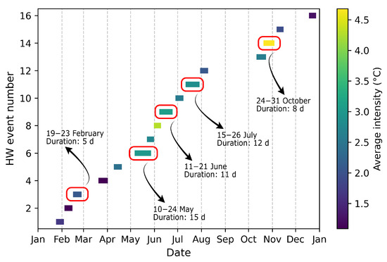
Figure 5.
HWs identified in 2022 characterised by their duration and average daily intensity. HWs selected for further analysis are signed with a red outline.
Candidate HWs for further analysis were then selected based on similar duration and intensity across different seasons, as well as the availability of satellite imagery. Five intense HW events in distinct seasons were chosen: 19–23 February, 10–24 May, 11–21 June, 15–26 July, and 24–31 October. Selected periods were characterised by mostly cloud-free weather, persistent high-pressure systems, and an absence of precipitation.
2.4. Computation of Predictors from Geospatial and EO Data
AT is influenced by factors such as surface material composition, urban geometry, and altitude, which affect how heat is stored, absorbed, and distributed across different landscapes [2,3]. To account for these influences, a relevant set of predictor variables (hereafter referred to as predictors) must be included for accurate temperature prediction. For this study, predictors were selected based on their physical relevance and influence on AT, derived from high-resolution spatial datasets or computed from EO data. Some meteorological variables, such as humidity, wind fields, and surface heat fluxes, which have a strong influence on AT, could not be included as high-resolution gridded products necessary for microscale assessment are unavailable. While LST is commonly used in similar studies [13,40,43,45,52], it was not employed here because the study area is larger than a single Landsat tile, preventing full spatial coverage at a consistent acquisition time and making it unsuitable for producing continuous, comparable predictors.
All predictors were obtained from open sources, ensuring the reproducibility of the interpolation method. Given the focus on seasonal HWs, selected predictors were categorised as either static or dynamic (Table 1). Static predictors remain constant over each HW, while dynamic predictors reflect seasonal variability. Static variables included Imperviousness Density (IMD), Sky View Factor (SVF), Canopy Height (CH), and Digital Terrain Model (DTM). DTM, IMD, and CH are available in analysis-ready format, while SVF was derived using building height data from the Lombardy and Piedmont regions and computed with the dedicated SAGA tool in QGIS software, version 3.34.

Table 1.
Overview of predictor variables used in the study. For predictor acronyms, refer to the text.
Dynamic predictors were derived from EO data, specifically Sentinel-2 MSI Level-2A bottom-of-atmosphere surface reflectance imagery. The primary advantage of EO data is its ability to capture seasonal land cover changes, such as those of vegetation, that directly influence AT. Furthermore, Sentinel-2 offers high spatial resolution and broad coverage, enabling it to fully encompass the study area. Five cloud-free scenes closest in time to each HW event were identified from the Copernicus Browser (https://browser.dataspace.copernicus.eu/, accessed on 9 May 2025) but processed on the Google Earth Engine (GEE), a cloud-based geospatial analysis platform [80]. Each scene was captured during or within six days of the start or end of an HW event: 25 February, 11 May, 10 June, 20 July, and 18 October. Product information for each scene can be found in Table A2. From these scenes, the following dynamic predictors were derived: SWIR-1 (Short-Wave Infrared), SWIR-2, Normalized Difference Vegetation Index (NDVI), and Local Climate Zones (LCZs). LCZ was the only dynamic predictor computed outside of GEE, following the combined remote sensing and GIS-based method of Vavassori et al. [79]. SWIR-1 and SWIR-2 were included due to their sensitivity to soil moisture, which can influence AT [61,81]. Finally, NDVI, a spectral index that indicates vegetation health, was calculated as NDVI = (B8 − B4)/(B8 + B4), B8 being the Near-Infrared (NIR) band and B4 being the Red band.
After computations, both static and dynamic predictors were resampled to a uniform spatial resolution of 20 m.
2.5. Material Abundance from Hyperspectral Data
Surface material properties significantly influence both LST and AT [2,3,4,14]. Traditionally, this relationship has been examined using static land cover classifications often coming from multispectral (MS) data, where each pixel is assigned a single class and is then compared to temperatures. In contrast, we propose comparing AT interpolation with material abundance maps derived from spectral unmixing of HS data. The latter offers advantages over MS data for detecting surface material properties by providing high spectral resolution with hundreds of narrow bands across a broad spectral range. In particular, spectral unmixing of HS data offers a more detailed and accurate representation of surface composition through per-pixel fractional abundances of materials [82,83,84]. Additionally, it allows us to assess surface characteristics relevant to thermal behaviour and quantify the cooling or warming influence of each material.
Our approach employs DLR Earth Sensing Imaging Spectrometer (DESIS), an advanced HS instrument aboard the International Space Station, jointly managed by Teledyne Brown Engineering, Alabama, USA, and the German Aerospace Center (DLR), Germany. DESIS covers the VNIR range from 400 to 1000 nm, with a spectral sampling distance of 2.55 nm, 235 spectral bands, and a 30 m spatial resolution [85]. One DESIS image, acquired on 6 June 2022, was retrieved from EOWEB GeoPortal (https://eoweb.dlr.de/egp/, accessed on 16 May 2025). A spectral window binning of 4 times was applied to this image, spectral binning being the summation of adjacent spectral bands, taking into account the spectral response functions [86]. The image is completely cloud-free; its footprint and RGB composite are shown in Figure 6. The co-registration was applied with the closest-in-time, cloud-free Sentinel-2 imagery from 10 June 2022, using the open-source Python package GeFolki [87]. Following that, geometric accuracy improved significantly.
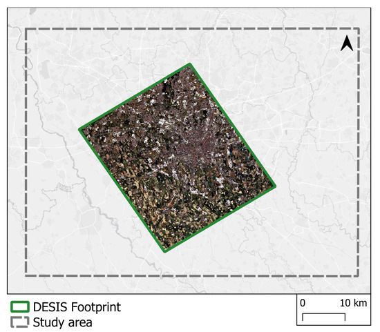
Figure 6.
DESIS footprint and RGB composite (bands R:27, G:17 and B:10) overlayed on the study area.
For spectral unmixing, we manually selected a set of pixels from the image to define the endmembers, choosing pixels that correspond to the purest (unmixed) possible surfaces. Endmember selection was based on their urban climate relevance, particularly their potential to mitigate or intensify heat. They represent common surface materials found in Milan and cities globally, enabling reproducible application of the method. Seven materials were selected accordingly, namely shingle, metal, and asphalt (artificial materials) and bare soil, low vegetation, tall vegetation, and water (natural materials). We then applied a least squares unmixing method to generate fractional abundance maps for these endmembers across the DESIS scene [82]. Two constraints were imposed, ensuring that abundances are non-negative (non-negativity constraint) and sum up to one within each pixel (full additive constraint). Following spectral unmixing, we compared abundance maps of all materials besides water with AT interpolation for June 2022.
2.6. AT Modelling
In this study, we apply the Random Forest (RF) regression algorithm for spatial prediction of AT due to its ability to model nonlinear interactions between predictors and its robustness to overfitting. This is particularly important for this work, given the complex relationships between AT and explanatory variables, e.g., land cover, elevation, and vegetation. RF has been successfully applied in previous studies [13,50,88], showing good predictive performance. While we primarily report from RF, we also tested other algorithms such as XGBoost, which showed lower performance. All modelling and statistical analysis were conducted using Python (version 3.11) and scikit-learn package [89].
In addition to selecting HW periods, we further divided each HW into five distinct diurnal and nocturnal phases, corresponding to different heating and cooling stages of the day, following the theoretical diurnal temperature cycle [3]. These phases were defined relative to sunrise, solar noon, and sunset, which vary by season. Table 2 shows phase acronyms, selected time intervals, and the number of available stations per HW and phase.
Table 2.
Diurnal/nocturnal phases for each HW period with corresponding time intervals and number of available stations. HP is the heating phase (early morning, 1–3 h after sunrise), WP is the warmest phase (2–4 h after solar noon), CP1 is cooling phase 1 (2 h before sunset), CP2 is cooling phase 2 (3–5 h after sunset), and MUHI is the period of maximum UHI (2 h before sunrise).
The number of available stations varied slightly across HWs and phases due to gaps in CML station records, but remained consistently above 91, except for October, when it dropped to about 85. This setup resulted in 25 unique modelling cases: five HWs combined with five diurnal/nocturnal phases. The stations were split into 70% for training the model and 30% for testing it. To maintain the representativeness of both samples, the split was based on stratified sampling, which ensured balanced coverage of urban and natural land cover zones and between ARPA and CML stations. This stratification is important for AT modelling, which is sensitive to land cover heterogeneity and sensor placement [90].
To account for the neighbourhood thermal influence, we computed focal statistics of each predictor within a buffer of 150 m radius around each station. This radius value was proposed by [13] as an optimal distance to achieve the highest model performance. Regarding the focal statistics, the focal mean was computed for continuous variables, and majority filtering was applied to categorical predictors, i.e., LCZ. All predictors were normalised using min–max scaling. Although normalisation is not strictly required for RF, this step ensured compatibility with other algorithms such as neural networks.
Hyperparameter tuning was performed in the model training phase to identify the optimal combination of model parameters for RF, as they can significantly influence the model performance. A randomised search over hyperparameters was performed using 5-fold cross-validation. In this way, we ensure generalisability and reduce overfitting by testing model performance on multiple training–validation splits. The hyperparameters tuned included number of trees (n_estimators), maximum tree depth (max_depth), number of features considered per split (max_features), and minimum samples required to split a node or form a leaf (min_samples_split, min_samples_leaf). The final model was trained using the hyperparameter combination that resulted in the lowest mean squared error.
Model performance was evaluated using the RMSE and the coefficient of determination () on the test set. RMSE quantifies prediction error, while indicates the proportion of variance in observed temperatures explained by the model. In addition, we analysed feature importance based on the impurity reduction achieved by each variable during splitting. This analysis was needed for understanding which predictors are most influential during different diurnal phases.
An overview of the research workflow summarising the information from each section is provided in Figure 7.
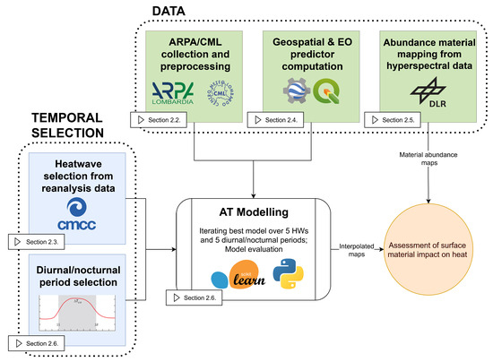
Figure 7.
Flowchart summarising the main research steps.
3. Results
3.1. Model Performance
The first set of analysis explores the model performance on the testing set based on the and RMSE values across the five HW events and the five diurnal and nocturnal phases considered in the present work. In particular, the distribution of is represented as a heatmap (Figure 8a), while the RMSE values are depicted in a barplot (Figure 8b).
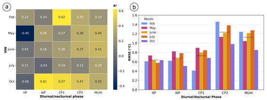
Figure 8.
(a) Heatmap showing values over all diurnal/nocturnal phases and for each HW; (b) barplot of RMSE values over all diurnal/nocturnal phases and for each HW. Black horizontal line shows mean RMSE for each phase.
From the heatmap, it appears that varies substantially across phases. Overall, the model performance is worse for the diurnal phases (HP and WP), corresponding to the morning and the warmest time of the day. In some cases, such as HP during May and October, and WP in July, values are even negative, indicating that the model failed to learn a meaningful relationship between predictors and AT. This underperformance is particularly evident for HP, while WP shows better results, even though the mapped ATs do not appear reliable. This aspect is further commented on in Section 4. Given these results, HP and WP are excluded from subsequent analysis and will not be used either to explore the spatial distribution of heat or draw connections to the impact of surface materials. On the other hand, phases CP1, CP2, and MUHI show more stable and reliable performance across HWs. CP1 (late afternoon to evening) achieves the highest , reaching up to 0.62 in February, but values in other HWs are closer to 0.2. Nighttime phases (CP2 and MUHI) are the most consistent, with typically above 0.3 across months, reaching up to 0.5.
Regarding the RMSE, a gradual increase is observed from morning (HP) to nighttime (CP2 and MUHI). HP and WP exhibit the lowest RMSE values, typically between 0.5 and 0.8 °C, which reflects the narrower temperature ranges during daytime. Conversely, higher RMSE values occur during nighttime phases, when urban–rural differences are more pronounced and the CUHI is stronger. Following that, CP2 and MUHI usually show RMSE values between 1.0 and 1.4 °C, which is double compared to daytime. February shows the highest errors during CP2, and October shows the lowest. Interestingly, this pattern reverses during the daytime. February and October, the two coolest months, show the lowest errors for WP and CP1, while for HP, the lowest error occurs narrowly in July. In general, during these phases, heatwaves in May, June, and July exhibit higher errors. Overall, late afternoon and nighttime periods experience higher , but also higher RMSE. Both metrics should be interpreted in conjunction with the produced AT maps and expected spatial patterns under calm, clear-sky conditions.
3.2. Feature Importance
The importance of each predictor, grouped by diurnal phases across HWs, is shown in Figure 9. A higher feature importance indicates a greater decrease in impurity, which in the regression context refers to the reduction in MSE. In particular, MSE indicates how far our AT predictions are from the actual values. The importance value of a feature indicates how useful each feature was in predicting AT on average across all trees in the forest.
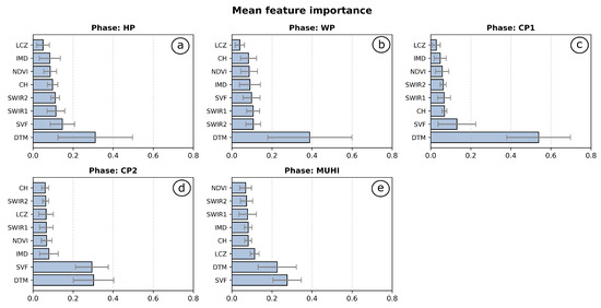
Figure 9.
Feature importance scores for all predictor variables, per phase (a–e). The importance values reflect how much each feature contributed to predicting AT, averaged across all trees in the forest. These are relative, unitless scores, normalised so that their sum equals one. The importances are averaged for each phase over all HWs, with SD indicated by ticks at the top of each bar.
Across most diurnal phases, DTM ranked as the most important predictor. This is particularly evident during the CP1 phase (Figure 9c), where DTM shows the highest reduction in importance, above 0.5. During other daytime phases, other predictors exhibit a relatively balanced importance, with no single feature approaching the influence of DTM. LCZs ranked as the least important predictor, followed by IMD and, somewhat unexpectedly, NDVI. Slightly higher importance was observed for SVF, SWIR-1, and SWIR-2, although their values remained significantly lower than those of DTM.
During nighttime, the ranking of predictor influence slightly changed (Figure 9d,e). The influence of urban morphology indicators, particularly SVF, LCZ, and IMD, begins to increase, while the DTM keeps standing as one of the most influential features. Notably, during MUHI, SVF is the most important predictor with a mean importance just under 0.3. A similar value is reported during CP2, when SVF ranks second after DTM. These findings indicate the influence of urban form on nocturnal AT patterns.
3.3. Seasonal and Diurnal Dynamics
In the next part of the analysis, the seasonal and diurnal AT dynamics are explored (Figure 10). Since 25 AT maps were produced, a detailed review of each would be too extensive. Instead, AT distribution plots are shown for three selected periods (CP1, CP2, and MUHI), following the exclusion of HP and WP phases due to low model performance. Figure 10 presents the distributions of AT values for 15 interpolated maps (five months for each phase). In addition, special focus is given to the June HW (see Figure 11), further discussed in Section 3.4, where material abundances are compared with AT.
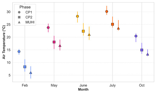
Figure 10.
AT distribution by phase (CP1, CP2, MUHI) across months. Each vertical line represents the full range (min–max) of temperatures, while markers denote the mean: circle for CP1, square for CP2, and triangle for MUHI. Colours correspond to months.
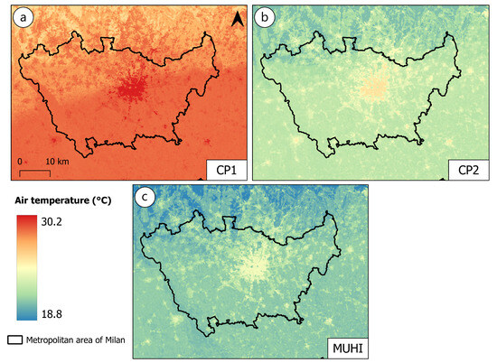
Figure 11.
Predicted AT maps for (a) CP1, (b) CP2, and (c) MUHI, relative to the June HW event.
The AT exhibits clear diurnal and seasonal patterns. The diurnal dynamics show that temperatures are highest during CP1 (afternoon cooling), drop significantly during CP2 (later evening), and reach their minimum during MUHI (pre-dawn). For example, in February, the mean temperature drops from 14.3 °C in CP1 to 6.1 °C during MUHI, reflecting a diurnal AT change of over 8 °C, which is the largest among all months. This progression highlights the transition from daytime heating to nighttime cooling and stabilisation before sunrise. From a seasonal perspective, the data follow expected trends. Mean AT within phases rises from February (6–14 °C) through May (16–24 °C) to the summer months of June and July (21–31 °C) and then declines in October (13–20 °C). Variability within phases, as indicated by SD and range, is generally moderate (SD 0.3–1.1 °C; range 2–5 °C), with slightly higher variability during the cooler months of February and May.
An example of predicted AT distribution over diurnal phases is shown in Figure 11, referring to the June HW event. While here only three maps are displayed, the reader is referred to Figure A1 for the full set of predicted AT maps. For all three phases, the central urban area is significantly warmer than its surroundings. The temperature difference between dense urban zones and forested areas is between 3 and 5 °C during the CP2 and MUHI phases (Figure 11b,c). During the CP1 (Figure 11a), this difference is somewhat smaller, and the effect of elevation is more visible, with the southern plain showing higher temperatures than the elevated northern zone. In CP2 and MUHI, smaller urban settlements also show higher temperatures compared to their agricultural surroundings. The coolest areas are the hills to the north and the well-vegetated Ticino River valley (in the south-west). Additionally, several central urban parks (such as Parco Sempione or Parco Indro Montanelli) experience lower AT values compared to their surrounding built-up zones. Using LCZ classes, these parks were delineated as LCZ A (dense trees), while LCZ 2, 3, 5, 8, and E were merged into a single class representing the dominant urban fabric in central Milan. Statistics computed for CP1, CP2, and MUHI show that the cooling effect of urban vegetation reaches around 1–2 °C compared to the combined urban class. Finally, it is interesting to note that during CP2 and MUHI, AT does not fall below 20 °C across most of the urbanised area. These conditions correspond to tropical nights, which have known implications for human health.
AT distributions across LCZs showed the highest values in compact and densely built-up classes, i.e., LCZ 2 and LCZ 3 (compact midrise and lowrise), as shown in Figure 12. The lowest AT values were consistently observed in vegetated zones, particularly LCZ A (dense trees) and LCZ B (scattered trees). The cooling effect of natural vegetated LCZs was slightly more pronounced during the nighttime phases, especially CP2 and MUHI, with temperature differences exceeding 3 °C when compared to compact classes, serving as a proxy for UHI magnitude.
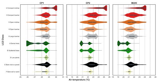
Figure 12.
Violin plots showing the distribution of AT, relative to the June HW, across LCZs for three different diurnal phases: CP1, CP2, and MUHI. Each violin represents the density distribution of AT for a given LCZ, with internal boxplots indicating the interquartile range and median. Temperature ranges on x-axis are the same for CP2 and MUHI, and different for CP1.
3.4. Surface Material Impact on Heat
As a final step in the analysis, we examined the relationship between the interpolated AT maps and surface material abundances derived from the spectral unmixing of DESIS HS data. The purpose of the analysis was to evaluate the added value of HS imagery for urban climate research, while enhancing the interpretability of the model outputs. The abundance maps for all materials considered in this study are provided in Figure A2. While materials are presented individually, they serve as proxies for broader land use categories. For instance, shingle characterises dense urban fabric; asphalt and metal correspond to industrial zones; bare soil reflects exposed, non-vegetated surfaces (often agricultural); and low and tall vegetation represents vegetated areas with varying cooling potential.
Figure 13 illustrates how AT varies across quartiles of each material’s abundance (ranging from 0 to 100%). For artificial materials, AT consistently increases with material fraction, from mixed pixels (Q1 and Q2) to more homogeneous ones (Q3 and Q4). This pattern is especially pronounced during nighttime phases (CP2 and MUHI).
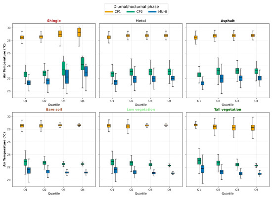
Figure 13.
AT distributions by phase (CP1, CP2, MUHI) based on surface material abundances derived from DESIS data, relative to the June HW event. Distributions are grouped by material abundance quartiles (ranging from 0 to 100%), where Q3 (50–75%) and Q4 (75–100%) represent pixels with high material purity, while Q1 (0–25%) and Q2 (25–50%) correspond to mixed or less dominant material compositions. The boxplots illustrate the distributions, where the interquartile range (Q1–Q3) is enclosed by the box, whiskers extend to the minimum and maximum AT, and the mean is indicated by the horizontal line.
Shingle shows the strongest warming effect, with mean AT increasing steadily from 28.5 °C in Q1 to 29.3 °C in Q4 during CP1 (+0.8 °C), and from 22.7 °C to 24.2 °C in CP2 (+1.5 °C), while in MUHI, it rises from 21.4 °C to 23.0 °C (+1.6 °C). Asphalt and metal follow similar trends, with CP1 means increasing from 28.5 °C to 28.8 °C (+0.3 °C) and nighttime values rising by about 0.5–0.7 °C between Q1 and Q4 (to 23.1 °C in CP2 and MUHI). In contrast, bare soil shows a slight cooling effect, with means decreasing from Q1 to Q4 during CP2 and MUHI, while daytime ATs remain stable. Further, vegetation abundance is associated with cooling. Low vegetation’s mean AT declines from 21.6 °C in Q1 to 21.1 °C in Q4 for MUHI (−0.5 °C), while tall vegetation drops from 21.8 °C to 20.9 °C (−0.9 °C) over the same quartiles. The absolute cooling effect is modest, likely due to the sparse dense tree cover within the DESIS footprint.
4. Discussion
In this study, we apply regression-based AT modelling in Milan and discuss the results in terms of their seasonal and diurnal or nocturnal variations during HWs that occurred in 2022. The predicted AT maps also reflect changes across different heating and cooling phases. This section provides a discussion on the results presented in Section 3.
Regression-based approaches for AT modelling have previously been applied in Italy [53,54,56]; however, to the best of our knowledge, this is the first study to implement such a method at a high spatial resolution, i.e., 20 m. Existing studies typically rely on coarser datasets for computing the predictors, often at a resolution of 1 km, which is insufficient for capturing the fine-scale heterogeneity of AT across urban environments. In contrast, our approach produced detailed AT maps capable of resolving intra-urban variability.
4.1. AT Modelling
AT modelling demonstrated notably better performance during late afternoon and nighttime periods (CP1, CP2 and MUHI), when the urban–rural differences are more pronounced and spatial temperature patterns are less complex (Figure 8). Our model achieved average values between 0.33 and 0.37 for those periods across all HWs, reflecting modest but reasonable performance under the challenging conditions of high-resolution urban modelling. Furthermore, the corresponding RMSE values ranged from approximately 0.7 °C for CP1 to 1.0–1.4 °C for CP2 and MUHI, indicating a good accuracy in temperature predictions.
In contrast, daytime AT modelling during the HP and WP remains challenging, leading to their exclusion from in-depth analysis. This is reflected in the lower model performance and aligns with findings in the literature. For instance, Venter et al. [48] reported an of 0.05 for predicting daily maximum AT in Oslo, comparable to the WP phase here. Similarly, Ho et al. [50] reported for maximum AT predictions. Other studies also noted the difficulty of daytime AT mapping due to radiative bias [44] or reported generally lower model performance during daytime compared to nighttime. For HP, our model ranged from negative to around 0.2, while the WP values ranged from 0 to 0.6. Despite an acceptable in WP, closer inspection revealed unrealistic spatial patterns, such as warmer than expected AT in dense vegetation. Comparable inconsistencies appeared in HP. Several factors likely explain this. Firstly, during HP, AT increases rapidly and is heavily shaped by microclimatic land cover variations [3]. The model’s lower predictive capacity may be due to the absence of meteorological predictors. Secondly, urban thermal fields during HP tend to be spatially homogeneous, with limited variability among stations, especially in summer. This is compounded by sparse sensor coverage in natural land covers, such as forests, further reducing data variability and weakening model performance.
Regarding the feature importance, DTM consistently ranked among the most important predictors in all phases and HW periods (Figure 9). Although the study area is mostly flat, the station elevations vary between 50 and 400 m, providing a significant, overall altitude difference. Some hilly terrain in the north, combined with a relatively even distribution of stations across the 50–400 m elevation range, helps ensure that DTM’s importance is not artificially increased due to clustered sampling. Nevertheless, such a strong influence is surprising and can be partly explained as a result of the multicollinearity between the other predictors, causing the model to rely on DTM for explanatory power. Additionally, SVF contributed significantly to the nighttime model accuracy by capturing the influence of urban form on nocturnal cooling (Figure 9d,e).
4.2. Interpretation of the AT Predictions
Considering CP1, CP2, and MUHI, the spatial patterns of the predicted AT during HWs reflected expected CUHI effects (Figure 11). In particular, central urban areas were persistently warmer than surrounding rural and vegetated zones by approximately 3–5 °C, which is consistent with prior research [15,49,91]. Densely vegetated zones recorded the lowest AT values, followed by agricultural fields, which demonstrate significant cooling through radiative heat loss [2]. Urban parks reduced AT by 1–2 °C relative to dense urban surroundings, in accordance with previous studies [92,93]. AT predictions were further evaluated using the LCZ framework, a widely recognised urban microclimate classification, which showed that compact built-up LCZs are approximately 3 °C warmer than densely vegetated ones (LCZ A), highlighting the value of our results for intra-urban heat pattern analysis. These results highlight how urban greenery mitigates extreme heat. Variations in AT during these phases were quite similar across all seasons and followed expected patterns.
The results discussed above are particularly significant from a public health perspective. HWs are periods of extreme heat stress that often lead to extremely warm nights, known as tropical nights, when temperatures remain above 20 °C. During these times, people are unable to cool down properly, which leads to an increase in heat-related health risks and mortality [9,10,94]. The high-resolution AT maps produced in this study can help identify urban heat hotspots during late afternoon and nighttime, providing city authorities with actionable information. Consequently, these maps could guide targeted urban greening or be combined with the spatial distribution of vulnerable populations, such as the elderly and children, supporting health-centred strategies to mitigate heat-related risks. Additionally, this study offers insights into winter HWs, which are often overlooked since the negative impacts of heat are predominantly experienced during summer. On the contrary, winter HWs may have some beneficial effects; however, this aspect is beyond the scope of the current research.
Another step in the analysis involved exploring the relationship between surface material abundances, estimated through the spectral unmixing of DESIS HS data, and the predicted AT maps. This work was carried out using a single DESIS image acquired close to the June HW period. The approach offers significant potential to overcome the limitations of traditional land cover classifications, which assign only a single class per pixel. Due to its high spectral resolution, HS data enables more accurate sub-pixel material abundance estimation. This is achieved with higher accuracy compared to MS data, which has a limited number of bands. While we focused on a single cloud-free DESIS image, this method can be replicated to other cloud-free periods and extended to other HS sensors. The results show that materials such as shingle, asphalt, and metal are associated with AT increases when comparing mixed pixels to those with material purity exceeding 75% (Figure 13). These materials serve as proxies for specific land uses, i.e., dense urban fabric and industrial areas. Conversely, increasing abundances of tall and low vegetation are associated with AT cooling, though this effect remains relatively modest (<1.0 °C). This is likely due to the spatial coverage of the DESIS tile, which is centred over the urban core and does not include the densely forested zones of the study area. As a result, the vegetation captured in the DESIS tile mostly represents sparse urban greenery, which generally has a lower cooling potential compared to densely vegetated areas [95].
4.3. Limitations and Future Outlook
Some additional limitations of the present study should be acknowledged, primarily related to data availability and model design. First, the approach relies on cloud-free Sentinel-2 imagery, which introduces a bias towards clear-sky conditions. As a result, predictions cannot be generated when satellite data are unavailable, and the temporal resolution is constrained by the Sentinel-2 revisit time. Also, model performance is inherently dependent on the predictors used. While the current selection achieves reasonable accuracy at night, future improvements could include additional variables such as surface albedo or soil moisture. Consequently, considerable work remains to enhance the estimation of daytime AT using data-driven approaches like the present methodology. High-resolution LST from Landsat satellites could also be incorporated, but over a smaller study area due to the extent of the Landsat tile (30 km × 30 km).
Moreover, although the weather network used in this study features nearly 100 sensors, well-distributed across the study area, a higher number of stations would help capture finer spatial variability, particularly across different land cover types. In this context, Netatmo CWSs could be considered to complement existing data [66], despite concerns related to their data quality and the lack of metadata on sensor placement [21,24]. In contrast, our current setup using ARPA and CML provides more controlled and reliable metadata.
HS imagery has been underutilised in urban climate research, despite the increasing availability from multiple missions in recent years. It offers opportunities to characterise urban surfaces at the sub-pixel level, beyond the capabilities of traditional MS data. This study serves as a proof of concept, demonstrating the feasibility and value of using HS data for urban climate applications. Further research should explore comparisons across different HS sensors, improve spectral unmixing techniques, and examine interactions of multiple materials within mixed pixels to better understand their influence on AT. Collectively, these findings highlight the strong potential of HS data to advance urban climate science.
5. Conclusions
This study employed ML regression-based modelling to estimate high-resolution AT during HWs in Milan in 2022, capturing fine-scale intra-urban temperature variability under extreme conditions. Modelling relied on a combination of authoritative and crowdsourced AT measurements, as well as predictors derived from geospatial and EO data. Further focus was given to examining seasonal and temporal changes of the daily AT cycle, as well as exploring the potential of HS imagery for urban climate applications. Prior to this study, no fine-scale mapping had been conducted in Milan. The results are relevant for urban heat risk assessment and adaptation planning. High-resolution AT maps can help in identifying heat exposure hotspots, particularly at night during HWs when ATs remain high.
The model showed consistently better performance during late afternoon and nighttime periods, with an average between 0.33 and 0.37, and RMSE ranging from 0.7 °C to 1.4 °C across HWs. In contrast, daytime predictions were less accurate, particularly during the morning heating phase and the warmest daily phase, when predicted AT patterns proved unreliable due to the complex urban thermal field. Spatial AT patterns during late afternoon and nighttime highlighted the UHI phenomenon, with some central urban zones being 3–5 °C warmer than vegetated and agricultural areas in all seasons. Urban parks demonstrated cooling effects of 1–2 °C, consistent with the literature.
This study offers a novel contribution by demonstrating that HS imagery can be successfully exploited to estimate surface material abundances through spectral unmixing and linking them to predicted AT. To our knowledge, it is the first application of HS imagery in urban climate research to explore how sub-pixel material fractions influence AT, and it could pave the way for many new applications of HS data in this domain. Our results showed that pixels dominated by shingle, asphalt, or metal experience an AT increase of up to 1.5 °C. Pixels with a higher abundance of low or tall vegetation were associated with a cooling effect, though more modest, below 1.0 °C. The integration of HS data provides further potential for understanding surface–atmosphere interactions.
Finally, the methodology developed in this study is transferable and can be applied to other European or global urban areas, provided similar AT observations and geospatial or EO predictor datasets are available. To support reuse, a GitHub repository is made available at https://github.com/zgelam0xb/AT_Interpolation.git (accessed on 3 October 2025).
Author Contributions
Conceptualization, M.Ž., A.V. and M.A.B.; Methodology, M.Ž., A.V. and M.A.B.; Software, M.Ž. and A.V.; Validation, M.Ž. and A.V.; Formal Analysis, M.Ž. and A.V.; Investigation, M.Ž. and A.V.; Resources, M.Ž. and A.V.; Data Curation, M.Ž. and A.V.; Writing—Original Draft Preparation, M.Ž. and A.V.; Writing—Review and Editing, M.Ž., A.V. and M.A.B.; Visualization, M.Ž. and A.V.; Supervision, A.V. and M.A.B.; Project Administration, M.A.B.; Funding Acquisition, M.A.B. All authors have read and agreed to the published version of the manuscript.
Funding
This study was carried out within the Space It Up project funded by the Italian Space Agency, ASI, and the Ministry of University and Research, MUR, under contract n. 2024-5-E.0-CUP n. I53D24000060005.
Data Availability Statement
ARPA network data is openly available from the dedicated website (https://www.arpalombardia.it/temi-ambientali/meteo-e-clima/form-richiesta-dati/, accessed on 24 April 2025). CML network data is not openly available and has been provided by CML on request. Geospatial and EO data are available from regional databases and over GEE: the full list of sources is reported in Table 1. DESIS is available on EOWeb Geoportal (https://eoweb.dlr.de/egp/, accessed on 16 May 2025). CMCC reanalysis data is openly available over the Data Delivery System (https://dds.cmcc.it/, accessed on 6 May 2025).
Acknowledgments
The authors acknowledge the CML association for providing the station data, with special thanks to Francesco Sudati and Matteo Negri for their support.
Conflicts of Interest
The authors declare no conflicts of interest.
Abbreviations
The following abbreviations are used in this manuscript:
| ARPA | Agenzia Regionale per la Protezione dell’Ambiente |
| AT | Air Temperature |
| CH | Canopy Height |
| CMCC | Euro-Mediterranean Center on Climate Change |
| CML | Centro Meteorologico Lombardo |
| CP | Cooling Phase |
| CUHI | Canopy-Layer Urban Heat Island |
| CWS | Citizen Weather Stations |
| DESIS | DLR Earth Sensing Imaging Spectrometer |
| DL | Deep Learning |
| DTM | Digital Terrain Model |
| EO | Earth Observation |
| ERA5 | ECMWF Reanalysis v5 |
| GEE | Google Earth Engine |
| HP | Heating Phase |
| HS | Hyperspectral |
| HW | Heatwave |
| IMD | Imperviousness Density |
| LCZ | Local Climate Zones |
| LST | Land Surface Temperature |
| ML | Machine Learning |
| MS | Multispectral |
| MUHI | Maximum UHI Phase |
| NDVI | Normalized Difference Vegetation Index |
| RF | Random Forest |
| RMSE | Root Mean Squared Error |
| SD | Standard Deviation |
| SUHI | Surface Urban Heat Island |
| SVF | Sky View Factor |
| SWIR | Short-Wave Infrared |
| UHI | Urban Heat Island |
| VHR-REA_IT | Very High-Resolution dynamical downscaling of ERA5 Reanalysis over Italy |
| WP | Warmest Phase |
Appendix A

Figure A1.
AT interpolated maps for all phases and HWs. Colour ramps are unique to each row.
Figure A1.
AT interpolated maps for all phases and HWs. Colour ramps are unique to each row.


Figure A2.
DESIS material abundances from spectral unmixing. Note: Water is displayed for completeness but was excluded from the AT comparison in this study.
Figure A2.
DESIS material abundances from spectral unmixing. Note: Water is displayed for completeness but was excluded from the AT comparison in this study.

Table A1.
Summary of the sixteen HWs observed in Milan during 2022. Cumulative intensity represents the cumulative excess heat above the long-term threshold for all HW days. Average intensity is the mean daily exceedance, and Deviation is the difference between each HW’s average intensity and the 2022 average.
| HW | Start | End | Duration (Days) | Cumulative Intensity (°C) | Average Intensity (°C) | Deviation (°C) |
|---|---|---|---|---|---|---|
| 1 | 28/01/2022 | 31/01/2022 | 4 | 6.7 | 1.7 | −0.8 |
| 2 | 08/02/2022 | 11/02/2022 | 4 | 4.4 | 1.1 | −1.4 |
| 3 | 19/02/2022 | 23/02/2022 | 5 | 10.4 | 2.1 | −0.4 |
| 4 | 24/03/2022 | 29/03/2022 | 6 | 6.5 | 1.1 | −1.4 |
| 5 | 13/04/2022 | 16/04/2022 | 4 | 9.7 | 2.4 | −0.1 |
| 6 | 10/05/2022 | 24/05/2022 | 15 | 45.1 | 3.0 | 0.5 |
| 7 | 26/05/2022 | 28/05/2022 | 3 | 8.3 | 2.8 | 0.3 |
| 8 | 04/06/2022 | 06/06/2022 | 3 | 12.8 | 4.3 | 1.8 |
| 9 | 11/06/2022 | 21/06/2022 | 11 | 34.0 | 3.1 | 0.6 |
| 10 | 02/07/2022 | 05/07/2022 | 4 | 10.3 | 2.6 | 0.1 |
| 11 | 15/07/2022 | 26/07/2022 | 12 | 34.3 | 2.9 | 0.4 |
| 12 | 03/08/2022 | 06/08/2022 | 4 | 8.3 | 2.1 | −0.4 |
| 13 | 15/10/2022 | 20/10/2022 | 6 | 15.7 | 2.6 | 0.1 |
| 14 | 24/10/2022 | 31/10/2022 | 8 | 37.4 | 4.7 | 2.2 |
| 15 | 10/11/2022 | 12/11/2022 | 3 | 5.8 | 1.9 | −0.5 |
| 16 | 22/12/2022 | 24/12/2022 | 3 | 3.8 | 1.3 | −1.2 |
| Average | 5.9 | 15.8 | 2.5 | |||
Table A2.
Sentinel-2 MSI: MultiSpectral Instrument, Level-2A (SR) imagery used for predictor preparation. Two tiles for each date were used to encompass the whole study area. Time is in UTC.
Table A2.
Sentinel-2 MSI: MultiSpectral Instrument, Level-2A (SR) imagery used for predictor preparation. Two tiles for each date were used to encompass the whole study area. Time is in UTC.
| Date | Product IDs | Local Acquisition Time |
|---|---|---|
| 25/02/2022 | S2B_MSIL2A_20220225T101909_N0510_R065_T32TNR_20240530T024453 S2B_MSIL2A_20220225T101909_N0510_R065_T32TMR_20240530T024453 | 10:19 a.m. |
| 11/05/2022 | S2A_MSIL2A_20220511T101601_N0510_R065_T32TNR_20240617T140748 S2A_MSIL2A_20220511T101601_N0510_R065_T32TMR_20240617T140748 | 10:16 a.m. |
| 10/06/2022 | S2A_MSIL2A_20220610T101611_N0510_R065_T32TNR_20240630T072225 S2A_MSIL2A_20220610T101611_N0510_R065_T32TMR_20240630T072225 | 10:16 a.m. |
| 20/07/2022 | S2A_MSIL2A_20220720T101611_N0510_R065_T32TNR_20240715T001059 S2A_MSIL2A_20220720T101611_N0510_R065_T32TMR_20240715T001059 | 10:16 a.m. |
| 18/10/2022 | S2A_MSIL2A_20221018T102031_N0510_R065_T32TNR_20240802T013810 S2A_MSIL2A_20221018T102031_N0510_R065_T32TMR_20240802T013810 | 10:20 a.m. |
References
- European Environment Agency. European Climate Risk Assessment. 2024. Available online: https://www.eea.europa.eu/en/analysis/publications/european-climate-risk-assessment (accessed on 25 July 2025).
- Oke, T.R. The energetic basis of the urban heat island. Q. J. R. Meteorol. Soc. 1982, 108, 1–24. [Google Scholar] [CrossRef]
- Oke, T.R.; Mills, G.; Christen, A.; Voogt, J.A. Urban Climates; Cambridge University Press: Cambridge, UK, 2017. [Google Scholar] [CrossRef]
- Voogt, J.A.; Oke, T.R. Thermal remote sensing of urban climates. Remote Sens. Environ. 2003, 86, 370–384. [Google Scholar] [CrossRef]
- Giorgi, F. Climate change hot-spots. Geophys. Res. Lett. 2006, 33, 8. [Google Scholar] [CrossRef]
- Ali, E.; Cramer, W.; Carnicer, J.; Georgopoulou, E.; Hilmi, N.J.M.; Le Cozannet, G.; Lionello, P. Cross-Chapter Paper 4: Mediterranean Region. In Climate Change 2022: Impacts, Adaptation and Vulnerability. Contribution of Working Group II to the Sixth Assessment Report of the Intergovernmental Panel on Climate Change; Pörtner, H.O., Roberts, D.C., Tignor, M., Poloczanska, E.S., Mintenbeck, K., Alegría, A., Craig, M., Langsdorf, S., Löschke, S., Möller, V., et al., Eds.; Cambridge University Press: Cambridge, UK; New York, NY, USA, 2022; pp. 2233–2272. [Google Scholar] [CrossRef]
- Domeisen, D.I.V.; Eltahir, E.A.B.; Fischer, E.M.; Knutti, R.; Perkins-Kirkpatrick, S.E.; Schär, C.; Seneviratne, S.I.; Weisheimer, A.; Wernli, H. Prediction and projection of heatwaves. Nat. Rev. Earth Environ. 2023, 4, 36–50. [Google Scholar] [CrossRef]
- Campbell, S.; Remenyi, T.A.; White, C.J.; Johnston, F.H. Heatwave and health impact research: A global review. Health Place 2018, 53, 210–218. [Google Scholar] [CrossRef]
- Xu, Z.; FitzGerald, G.; Guo, Y.; Jalaludin, B.; Tong, S. Impact of heatwave on mortality under different heatwave definitions: A systematic review and meta-analysis. Environ. Int. 2016, 89–90, 193–203. [Google Scholar] [CrossRef]
- Ballester, J.; Quijal-Zamorano, M.; Méndez Turrubiates, R.F.; Pegenaute, F.; Herrmann, F.R.; Robine, J.M.; Basagaña, X.; Tonne, C.; Antó, J.M.; Achebak, H. Heat-related mortality in Europe during the summer of 2022. Nat. Med. 2023, 29, 1857–1866. [Google Scholar] [CrossRef]
- Zakšek, K.; Oštir, K. Downscaling land surface temperature for urban heat island diurnal cycle analysis. Remote Sens. Environ. 2012, 117, 114–124. [Google Scholar] [CrossRef]
- Schwarz, N.; Lautenbach, S.; Seppelt, R. Exploring indicators for quantifying surface urban heat islands of European cities with MODIS land surface temperatures. Remote Sens. Environ. 2011, 115, 3175–3186. [Google Scholar] [CrossRef]
- Venter, Z.S.; Chakraborty, T.; Lee, X. Crowdsourced air temperatures contrast satellite measures of the urban heat island and its mechanisms. Sci. Adv. 2021, 7, eabb9569. [Google Scholar] [CrossRef]
- Naserikia, M.; Nazarian, N.; Hart, M.A.; Sismanidis, P.; Kittner, J.; Bechtel, B. Multi-city analysis of satellite surface temperature compared to crowdsourced air temperature. Environ. Res. Lett. 2024, 19, 124063. [Google Scholar] [CrossRef]
- Verdonck, M.L.; Demuzere, M.; Hooyberghs, H.; Beck, C.; Cyrys, J.; Schneider, A.; Dewulf, R.; Van Coillie, F. The potential of local climate zones maps as a heat stress assessment tool, supported by simulated air temperature data. Landsc. Urban Plan. 2018, 178, 183–197. [Google Scholar] [CrossRef]
- Wang, K.; Jiang, S.; Wang, J.; Zhou, C.; Wang, X.; Lee, X. Comparing the diurnal and seasonal variabilities of atmospheric and surface urban heat islands based on the Beijing urban meteorological network. J. Geophys. Res. Atmos. 2017, 122, 2131–2154. [Google Scholar] [CrossRef]
- Cui, Y.Y.; Foy, B.d. Seasonal Variations of the Urban Heat Island at the Surface and the Near-Surface and Reductions due to Urban Vegetation in Mexico City. J. Appl. Meteorol. Climatol. 2012, 51, 855–868. [Google Scholar] [CrossRef]
- Oke, T. The distinction between canopy and boundary-layer urban heat islands. Atmosphere 1976, 14, 268–277. [Google Scholar] [CrossRef]
- World Meteorological Organization. Guide to Instruments and Methods of Observation (WMO-No. 8) | World Meteorological Organization. Available online: https://library.wmo.int/records/item/68695-guide-to-instruments-and-methods-of-observation?offset= (accessed on 25 July 2025).
- Muller, C.L.; Chapman, L.; Grimmond, C.S.B.; Young, D.T.; Cai, X. Sensors and the city: A review of urban meteorological networks. Int. J. Climatol. 2013, 33, 1585–1600. [Google Scholar] [CrossRef]
- Meier, F.; Fenner, D.; Grassmann, T.; Otto, M.; Scherer, D. Crowdsourcing air temperature from citizen weather stations for urban climate research. Urban Clim. 2017, 19, 170–191. [Google Scholar] [CrossRef]
- Potgieter, J.; Nazarian, N.; Lipson, M.J.; Hart, M.A.; Ulpiani, G.; Morrison, W.; Benjamin, K. Combining High-Resolution Land Use Data with Crowdsourced Air Temperature to Investigate Intra-Urban Microclimate. Front. Environ. Sci. 2021, 9, 720323. [Google Scholar] [CrossRef]
- Coney, J.; Pickering, B.; Dufton, D.; Lukach, M.; Brooks, B.; Neely III, R.R. How useful are crowdsourced air temperature observations? An assessment of Netatmo stations and quality control schemes over the United Kingdom. Meteorol. Appl. 2022, 29, e2075. [Google Scholar] [CrossRef]
- Napoly, A.; Grassmann, T.; Meier, F.; Fenner, D. Development and Application of a Statistically-Based Quality Control for Crowdsourced Air Temperature Data. Front. Earth Sci. 2018, 6, 118. [Google Scholar] [CrossRef]
- Fenner, D.; Bechtel, B.; Demuzere, M.; Kittner, J.; Meier, F. CrowdQC+—A Quality-Control for Crowdsourced Air-Temperature Observations Enabling World-Wide Urban Climate Applications. Front. Environ. Sci. 2021, 9, 720747. [Google Scholar] [CrossRef]
- Leconte, F.; Bouyer, J.; Claverie, R.; Pétrissans, M. Using Local Climate Zone scheme for UHI assessment: Evaluation of the method using mobile measurements. Build. Environ. 2015, 83, 39–49. [Google Scholar] [CrossRef]
- Emery, J.; Pohl, B.; Crétat, J.; Richard, Y.; Pergaud, J.; Rega, M.; Zito, S.; Dudek, J.; Vairet, T.; Joly, D.; et al. How local climate zones influence urban air temperature: Measurements by bicycle in Dijon, France. Urban Clim. 2021, 40, 101017. [Google Scholar] [CrossRef]
- Tsin, P.K.; Knudby, A.; Krayenhoff, E.S.; Ho, H.C.; Brauer, M.; Henderson, S.B. Microscale mobile monitoring of urban air temperature. Urban Clim. 2016, 18, 58–72. [Google Scholar] [CrossRef]
- Lehnert, M.; Geletič, J.; Dobrovolný, P.; Jurek, M. Temperature differences among local climate zones established by mobile measurements in two central European cities. Clim. Res. 2018, 75, 53–64. [Google Scholar] [CrossRef]
- Hersbach, H.; Bell, B.; Berrisford, P.; Hirahara, S.; Horányi, A.; Muñoz-Sabater, J.; Nicolas, J.; Peubey, C.; Radu, R.; Schepers, D.; et al. The ERA5 global reanalysis. Q. J. R. Meteorol. Soc. 2020, 146, 1999–2049. [Google Scholar] [CrossRef]
- Muñoz-Sabater, J.; Dutra, E.; Agustí-Panareda, A.; Albergel, C.; Arduini, G.; Balsamo, G.; Boussetta, S.; Choulga, M.; Harrigan, S.; Hersbach, H.; et al. ERA5-Land: A state-of-the-art global reanalysis dataset for land applications. Earth Syst. Sci. Data 2021, 13, 4349–4383. [Google Scholar] [CrossRef]
- UERRA. Regional Reanalysis for Europe on Single Levels from 1961 to 2019. Available online: https://cds.climate.copernicus.eu/datasets/reanalysis-uerra-europe-single-levels?tab=documentation (accessed on 25 July 2025).
- Krähenmann, S.; Walter, A.; Brienen, S.; Imbery, F.; Matzarakis, A. High-resolution grids of hourly meteorological variables for Germany. Theor. Appl. Climatol. 2018, 131, 899–926. [Google Scholar] [CrossRef]
- Devers, A.; Vidal, J.P.; Lauvernet, C.; Vannier, O. FYRE Climate: A high-resolution reanalysis of daily precipitation and temperature in France from 1871 to 2012. Clim. Past 2021, 17, 1857–1879. [Google Scholar] [CrossRef]
- Raffa, M.; Reder, A.; Marras, G.F.; Mancini, M.; Scipione, G.; Santini, M.; Mercogliano, P. VHR-REA_IT Dataset: Very High Resolution Dynamical Downscaling of ERA5 Reanalysis over Italy by COSMO-CLM. Data 2021, 6, 88. [Google Scholar] [CrossRef]
- Chen, F.; Kusaka, H.; Bornstein, R.; Ching, J.; Grimmond, C.S.B.; Grossman-Clarke, S.; Loridan, T.; Manning, K.W.; Martilli, A.; Miao, S.; et al. The integrated WRF/urban modelling system: Development, evaluation, and applications to urban environmental problems. Int. J. Climatol. 2011, 31, 273–288. [Google Scholar] [CrossRef]
- Maronga, B.; Gross, G.; Raasch, S.; Banzhaf, S.; Forkel, R.; Heldens, W.; Kanani-Sühring, F.; Matzarakis, A.; Mauder, M.; Pavlik, D.; et al. Development of a new urban climate model based on the model PALM—Project overview, planned work, and first achievements. Meteorol. Z. 2019, 28, 105–119. [Google Scholar] [CrossRef]
- De Ridder, K.; Lauwaet, D.; Maiheu, B. UrbClim—A fast urban boundary layer climate model. Urban Clim. 2015, 12, 21–48. [Google Scholar] [CrossRef]
- Trusilova, K.; Schubert, S.; Wouters, H.; Früh, B.; Grossman-Clarke, S.; Demuzere, M.; Becker, P. The urban land use in the COSMO-CLM model: A comparison of three parameterizations for Berlin. Meteorol. Z. 2016, 25, 231–244. [Google Scholar] [CrossRef]
- Hassani, A.; Santos, G.S.; Schneider, P.; Castell, N. Interpolation, Satellite-Based Machine Learning, or Meteorological Simulation? A Comparison Analysis for Spatio-temporal Mapping of Mesoscale Urban Air Temperature. Environ. Model. Assess. 2024, 29, 291–306. [Google Scholar] [CrossRef]
- Frustaci, G.; Pilati, S.; Lavecchia, C.; Montoli, E.M. High-Resolution Gridded Air Temperature Data for the Urban Environment: The Milan Data Set. Forecasting 2022, 4, 238–261. [Google Scholar] [CrossRef]
- Zhang, Z.; Du, Q. A Bayesian Kriging Regression Method to Estimate Air Temperature Using Remote Sensing Data. Remote Sens. 2019, 11, 767. [Google Scholar] [CrossRef]
- Wang, M.; He, G.; Zhang, Z.; Wang, G.; Zhang, Z.; Cao, X.; Wu, Z.; Liu, X. Comparison of Spatial Interpolation and Regression Analysis Models for an Estimation of Monthly Near Surface Air Temperature in China. Remote Sens. 2017, 9, 1278. [Google Scholar] [CrossRef]
- Burger, M.; Gubler, M.; Brönnimann, S. High-resolution dataset of nocturnal air temperatures in Bern, Switzerland (2007–2022). Geosci. Data J. 2024, 11, 623–637. [Google Scholar] [CrossRef]
- Benali, A.; Carvalho, A.C.; Nunes, J.P.; Carvalhais, N.; Santos, A. Estimating air surface temperature in Portugal using MODIS LST data. Remote Sens. Environ. 2012, 124, 108–121. [Google Scholar] [CrossRef]
- Wicki, A.; Parlow, E.; Feigenwinter, C. Evaluation and Modeling of Urban Heat Island Intensity in Basel, Switzerland. Climate 2018, 6, 55. [Google Scholar] [CrossRef]
- Zhang, Z.; Du, Q. Hourly mapping of surface air temperature by blending geostationary datasets from the two-satellite system of GOES-R series. ISPRS J. Photogramm. Remote Sens. 2022, 183, 111–128. [Google Scholar] [CrossRef]
- Venter, Z.S.; Brousse, O.; Esau, I.; Meier, F. Hyperlocal mapping of urban air temperature using remote sensing and crowdsourced weather data. Remote Sens. Environ. 2020, 242, 111791. [Google Scholar] [CrossRef]
- Zumwald, M.; Knüsel, B.; Bresch, D.N.; Knutti, R. Mapping urban temperature using crowd-sensing data and machine learning. Urban Clim. 2021, 35, 100739. [Google Scholar] [CrossRef]
- Ho, H.C.; Knudby, A.; Sirovyak, P.; Xu, Y.; Hodul, M.; Henderson, S.B. Mapping maximum urban air temperature on hot summer days. Remote Sens. Environ. 2014, 154, 38–45. [Google Scholar] [CrossRef]
- Tran, D.P.; Liou, Y.A. Creating a spatially continuous air temperature dataset for Taiwan using thermal remote-sensing data and machine learning algorithms. Ecol. Indic. 2024, 158, 111469. [Google Scholar] [CrossRef]
- Dos Santos, R.S. Estimating spatio-temporal air temperature in London (UK) using machine learning and earth observation satellite data. Int. J. Appl. Earth Obs. Geoinf. 2020, 88, 102066. [Google Scholar] [CrossRef]
- Cecilia, A.; Casasanta, G.; Petenko, I.; Argentini, S. A Machine Learning Algorithm to Convert Geostationary Satellite LST to Air Temperature Using In Situ Measurements: A Case Study in Rome and High-Resolution Spatio-Temporal UHI Analysis. Remote Sens. 2025, 17, 468. [Google Scholar] [CrossRef]
- Pichierri, M.; Bonafoni, S.; Biondi, R. Satellite air temperature estimation for monitoring the canopy layer heat island of Milan. Remote Sens. Environ. 2012, 127, 130–138. [Google Scholar] [CrossRef]
- Anniballe, R.; Bonafoni, S.; Pichierri, M. Spatial and temporal trends of the surface and air heat island over Milan using MODIS data. Remote Sens. Environ. 2014, 150, 163–171. [Google Scholar] [CrossRef]
- Colaninno, N.; Morello, E. Towards an operational model for estimating day and night instantaneous near-surface air temperature for urban heat island studies: Outline and assessment. Urban Clim. 2022, 46, 101320. [Google Scholar] [CrossRef]
- Kottek, M.; Grieser, J.; Beck, C.; Rudolf, B.; Rubel, F. World Map of the Köppen-Geiger climate classification updated. Meteorol. Z. 2006, 15, 259–263. [Google Scholar] [CrossRef]
- Rubel, F.; Brugger, K.; Haslinger, K.; Auer, I. The climate of the European Alps: Shift of very high resolution Köppen-Geiger climate zones 1800–2100. Meteorol. Z. 2017, 26, 115–125. [Google Scholar] [CrossRef]
- Demography in Figures–Resident Population. Italian National Institute of Statistics. Available online: https://demo.istat.it/app/?i=POS&l=en (accessed on 29 September 2025).
- Montanari, A.; Nguyen, H.; Rubinetti, S.; Ceola, S.; Galelli, S.; Rubino, A.; Zanchettin, D. Why the 2022 Po River drought is the worst in the past two centuries. Sci. Adv. 2023, 9, eadg8304. [Google Scholar] [CrossRef]
- Tabassum, A.; Hong, S.H.; Park, K.; Baik, J.J. Impacts of Changes in Soil Moisture on Urban Heat Islands and Urban Breeze Circulations: Idealized Ensemble Simulations. Asia-Pac. J. Atmos. Sci. 2024, 60, 541–553. [Google Scholar] [CrossRef]
- Šećerov, I.; Savić, S.; Milošević, D.; Marković, V.; Bajšanski, I. Development of an automated urban climate monitoring system in Novi Sad (Serbia). Geogr. Pannonica 2015, 19, 174–183. [Google Scholar] [CrossRef]
- Gubler, M.; Christen, A.; Remund, J.; Brönnimann, S. Evaluation and application of a low-cost measurement network to study intra-urban temperature differences during summer 2018 in Bern, Switzerland. Urban Clim. 2021, 37, 100817. [Google Scholar] [CrossRef]
- Foissard, X.; Dubreuil, V.; Quénol, H. Defining scales of the land use effect to map the urban heat island in a mid-size European city: Rennes (France). Urban Clim. 2019, 29, 100490. [Google Scholar] [CrossRef]
- Lelovics, E.; Unger, J.; Gál, T.; Gál, C.V. Design of an urban monitoring network based on Local Climate Zone mapping and temperature pattern modelling. Clim. Res. 2014, 60, 51–62. [Google Scholar] [CrossRef]
- Netatmo. Netatmo Weather Station. 2025. Available online: https://www.netatmo.com/en-gb (accessed on 19 July 2025).
- Davis Instruments. Vantage Pro2 Spec Sheets. 2025. Available online: https://support.davisinstruments.com/category/esfbscicgu-vantage-pro-2 (accessed on 24 July 2025).
- Chapman, L.; Bell, C.; Bell, S. Can the crowdsourcing data paradigm take atmospheric science to a new level? A case study of the urban heat island of London quantified using Netatmo weather stations. Int. J. Climatol. 2017, 37, 3597–3605. [Google Scholar] [CrossRef]
- Puche, M.; Vavassori, A.; Brovelli, M.A. Insights into the Effect of Urban Morphology and Land Cover on Land Surface and Air Temperatures in the Metropolitan City of Milan (Italy) Using Satellite Imagery and In Situ Measurements. Remote Sens. 2023, 15, 733. [Google Scholar] [CrossRef]
- Barriopedro, D.; García-Herrera, R.; Ordóñez, C.; Miralles, D.G.; Salcedo-Sanz, S. Heat Waves: Physical Understanding and Scientific Challenges. Rev. Geophys. 2023, 61, e2022RG000780. [Google Scholar] [CrossRef]
- Russo, S.; Dosio, A.; Graversen, R.G.; Sillmann, J.; Carrao, H.; Dunbar, M.B.; Singleton, A.; Montagna, P.; Barbola, P.; Vogt, J.V. Magnitude of extreme heat waves in present climate and their projection in a warming world. J. Geophys. Res. Atmos. 2014, 119, 12500–12512. [Google Scholar] [CrossRef]
- Perkins, S.E.; Alexander, L.V. On the Measurement of Heat Waves. J. Clim. 2013, 26, 4500–4517. [Google Scholar] [CrossRef]
- Perkins-Kirkpatrick, S.E.; Lewis, S.C. Increasing trends in regional heatwaves. Nat. Commun. 2020, 11, 3357. [Google Scholar] [CrossRef]
- Rousi, E.; Kornhuber, K.; Beobide-Arsuaga, G.; Luo, F.; Coumou, D. Accelerated western European heatwave trends linked to more-persistent double jets over Eurasia. Nat. Commun. 2022, 13, 3851. [Google Scholar] [CrossRef]
- Rockel, B.; Will, A.; Hense, A. The Regional Climate Model COSMO-CLM (CCLM). Meteorol. Z. 2008, 17, 347–348. [Google Scholar] [CrossRef]
- Garbero, V.; Milelli, M.; Bucchignani, E.; Mercogliano, P.; Varentsov, M.; Rozinkina, I.; Rivin, G.; Blinov, D.; Wouters, H.; Schulz, J.P.; et al. Evaluating the Urban Canopy Scheme TERRA_URB in the COSMO Model for Selected European Cities. Atmosphere 2021, 12, 237. [Google Scholar] [CrossRef]
- Adinolfi, M.; Raffa, M.; Reder, A.; Mercogliano, P. Investigation on potential and limitations of ERA5 Reanalysis downscaled on Italy by a convection-permitting model. Clim. Dyn. 2023, 61, 4319–4342. [Google Scholar] [CrossRef]
- Cavalleri, F.; Viterbo, F.; Brunetti, M.; Bonanno, R.; Manara, V.; Lussana, C.; Lacavalla, M.; Maugeri, M. Inter-comparison and validation of high-resolution surface air temperature reanalysis fields over Italy. Int. J. Climatol. 2024, 44, 2681–2700. [Google Scholar] [CrossRef]
- Vavassori, A.; Oxoli, D.; Venuti, G.; Brovelli, M.A.; Siciliani de Cumis, M.; Sacco, P.; Tapete, D. A combined Remote Sensing and GIS-based method for Local Climate Zone mapping using PRISMA and Sentinel-2 imagery. Int. J. Appl. Earth Obs. Geoinf. 2024, 131, 103944. [Google Scholar] [CrossRef]
- Gorelick, N.; Hancher, M.; Dixon, M.; Ilyushchenko, S.; Thau, D.; Moore, R. Google Earth Engine: Planetary-scale geospatial analysis for everyone. Remote Sens. Environ. 2017, 202, 18–27. [Google Scholar] [CrossRef]
- Sadeghi, M.; Babaeian, E.; Tuller, M.; Jones, S.B. The optical trapezoid model: A novel approach to remote sensing of soil moisture applied to Sentinel-2 and Landsat-8 observations. Remote Sens. Environ. 2017, 198, 52–68. [Google Scholar] [CrossRef]
- Shi, C.; Wang, L. Incorporating spatial information in spectral unmixing: A review. Remote Sens. Environ. 2014, 149, 70–87. [Google Scholar] [CrossRef]
- Heylen, R.; Parente, M.; Gader, P. A Review of Nonlinear Hyperspectral Unmixing Methods. IEEE J. Sel. Top. Appl. Earth Obs. Remote Sens. 2014, 7, 1844–1868. [Google Scholar] [CrossRef]
- Bioucas-Dias, J.M.; Plaza, A.; Dobigeon, N.; Parente, M.; Du, Q.; Gader, P.; Chanussot, J. Hyperspectral Unmixing Overview: Geometrical, Statistical, and Sparse Regression-Based Approaches. IEEE J. Sel. Top. Appl. Earth Obs. Remote Sens. 2012, 5, 354–379. [Google Scholar] [CrossRef]
- Krutz, D.; Müller, R.; Knodt, U.; Günther, B.; Walter, I.; Sebastian, I.; Säuberlich, T.; Reulke, R.; Carmona, E.; Eckardt, A.; et al. The Instrument Design of the DLR Earth Sensing Imaging Spectrometer (DESIS). Sensors 2019, 19, 1622. [Google Scholar] [CrossRef]
- DLR. DESIS data Products. 2025. Available online: https://www.dlr.de/de/eoc/forschung-transfer/projekte-und-missionen/desis/products/data-products (accessed on 31 July 2025).
- Brigot, G.; Colin-Koeniguer, E.; Plyer, A.; Janez, F. Adaptation and Evaluation of an Optical Flow Method Applied to Coregistration of Forest Remote Sensing Images. IEEE J. Sel. Top. Appl. Earth Obs. Remote Sens. 2016, 9, 2923–2939. [Google Scholar] [CrossRef]
- Chen, S.; Yang, Y.; Deng, F.; Zhang, Y.; Liu, D.; Liu, C.; Gao, Z. A high-resolution monitoring approach of canopy urban heat island using a random forest model and multi-platform observations. Atmos. Meas. Tech. 2022, 15, 735–756. [Google Scholar] [CrossRef]
- Pedregosa, F.; Varoquaux, G.; Gramfort, A.; Michel, V.; Thirion, B.; Grisel, O.; Blondel, M.; Prettenhofer, P.; Weiss, R.; Dubourg, V.; et al. Scikit-learn: Machine Learning in Python. J. Mach. Learn. Res. 2011, 12, 2825–2830. [Google Scholar]
- Sakthivel, P.; Sengupta, R. Spatial bias in placement of citizen and conventional weather stations and their impact on urban climate research: A case study of the Urban Heat Island effect in Canada. Urban Clim. 2025, 59, 102280. [Google Scholar] [CrossRef]
- Sanchez, B.; Roth, M.; Patel, P.; Simón-Moral, A. Application of a Semi-Empirical Approach to Map Maximum Urban Heat Island Intensity in Singapore. Sustainability 2023, 15, 12834. [Google Scholar] [CrossRef]
- Bowler, D.E.; Buyung-Ali, L.; Knight, T.M.; Pullin, A.S. Urban greening to cool towns and cities: A systematic review of the empirical evidence. Landsc. Urban Plan. 2010, 97, 147–155. [Google Scholar] [CrossRef]
- De Pauw, K.; Depauw, L.; Calders, K.; Caluwaerts, S.; Cousins, S.A.O.; De Lombaerde, E.; Diekmann, M.; Frey, D.; Lenoir, J.; Meeussen, C.; et al. Urban forest microclimates across temperate Europe are shaped by deep edge effects and forest structure. Agric. For. Meteorol. 2023, 341, 109632. [Google Scholar] [CrossRef]
- Conti, S.; Meli, P.; Minelli, G.; Solimini, R.; Toccaceli, V.; Vichi, M.; Beltrano, C.; Perini, L. Epidemiologic study of mortality during the Summer 2003 heat wave in Italy. Environ. Res. 2005, 98, 390–399. [Google Scholar] [CrossRef]
- Kraemer, R.; Kabisch, N. Parks Under Stress: Air Temperature Regulation of Urban Green Spaces Under Conditions of Drought and Summer Heat. Front. Environ. Sci. 2022, 10, 849965. [Google Scholar] [CrossRef]


Disclaimer/Publisher’s Note: The statements, opinions and data contained in all publications are solely those of the individual author(s) and contributor(s) and not of MDPI and/or the editor(s). MDPI and/or the editor(s) disclaim responsibility for any injury to people or property resulting from any ideas, methods, instructions or products referred to in the content. |
© 2025 by the authors. Licensee MDPI, Basel, Switzerland. This article is an open access article distributed under the terms and conditions of the Creative Commons Attribution (CC BY) license (https://creativecommons.org/licenses/by/4.0/).