A High-Resolution Sea Ice Concentration Retrieval from Ice-WaterNet Using Sentinel-1 SAR Imagery in Fram Strait, Arctic

Highlights

What are the main findings?

• We propose Ice-WaterNet, a novel superpixel-based deep learning framework that effectively reduces classification uncertainty in complex melt season conditions by integrating CRF and a dual-attention U-Net mechanism.
• The model is validated on 2735 Sentinel-1 SAR images from 2021–2023 in the Fram Strait, demonstrating superior performance over state-of-the-art methods in both winter and summer seasons across multiple evaluation metrics.

What is the implication of the main finding?

• This study indicates the critical need to develop high-resolution SAR-based products, which can more accurately capture fine-grained spatiotemporal melt characteristics and provide reliable data for climate change research and sea ice trend analysis.
• By revealing the limitations of passive microwave sensors in assessing melt conditions, this study emphasizes that high-resolution SIC retrieval is essential to reduce underestimation errors and support operational applications such as maritime navigation and polar environment monitoring with improved spatial and temporal precision.

Abstract

High spatial resolution sea ice concentration (SIC) is crucial for global climate and marine activity. However, retrieving high spatial resolution SIC from passive microwave sensors is challenging due to the trade-off between spatial resolution and atmospheric contamination. Our study develops the Ice-WaterNet framework, a novel superpixel-based deep learning model that integrates Conditional Random Fields (CRF) with a dual-attention U-Net to enhance ice–water classification in Synthetic Aperture Radar (SAR) imagery. The Ice-WaterNet model has been extensively tested on 2735 Sentinel-1 dual-polarized SAR images from 2021 to 2023, covering both winter and summer seasons in the Fram Strait. To tackle the complex surface features during the melt season, wind-roughened open water, and varying ice floe sizes, a superpixel strategy is employed to efficiently reduce classification uncertainty. Uncertain superpixels identified by CRF are iteratively refined using the U-Net attention mechanism. Experimental results demonstrate that Ice-WaterNet achieves significant improvements in classification accuracy, outperforming CRF and U-Net by 3.375% in Intersection over Union (IoU) and 3.09% in F1-score during the melt season, and by 1.96 in IoU and 1.75 in F1-score during the freeze season. The derived high-resolution SIC products, updated every two days, were evaluated against Met Norway ice charts and compared with ASI from AMSR-2 and SSM/I, showing a substantial reduction in misclassification in marginal ice zones, particularly under melting conditions. These findings underscore the potential of Ice-WaterNet in supporting precise sea ice monitoring and climate change research.

1. Introduction

In recent years, as the number of Synthetic Aperture Radar (SAR) images available for operational sea ice monitoring has increased with the SAR satellite launch such as ERS-1/2, RADARSAT-1/2, and Sentinel 1A/B, machine learning (ML) and deep learning (DL) techniques have been extensively investigated to distinguish between sea ice and open water (Asadi et al., 2021; Chen et al., 2024) [1,2]. Ice–water classification aims to extract ice-water pixels from remotely sensed (RS) imagery, based on which high-resolution sea ice concentration (SIC) products can be retrieved. SIC plays an important role in applications such as meteorological modeling, marine resources, and shipping route planning (Wu et al., 2022; Huang et al., 2023) [3,4].

Although previous studies have made progress in ice–water classification, only a limited number have explicitly incorporated the concept of uncertainty, particularly under complex and dynamic sea ice conditions. For instance, Asadi et al. (2021) integrated uncertainty estimation within a multilayer perceptron (MLP) neural network to improve automatic ice–water classification [1]. However, their approach primarily addressed model parameter uncertainty and feature-level ambiguity without systematically quantifying or reducing classification uncertainty at a structural level, especially for superpixels with mixed or ambiguous backscattering characteristics. Similarly, other deep learning frameworks have focused on enhancing feature extraction or multi-scale segmentation but often lack a dedicated mechanism to iteratively identify and refine highly uncertain regions arising from thin ice, wind-roughened water, or melt ponds. These limitations become particularly pronounced during the melting season, where high intra-class variability and rapidly changing surface conditions exacerbate classification ambiguity.

SIC can also be retrieved from passive microwave (PMW) remote sensing, which has the advantages of large-scale coverage and high temporal resolution. The traditional SIC retrieval algorithm from PMW remote sensing, such as the ARTSIST Sea Ice (ASI) and NASA Team (NT) algorithms, introduces uncertainty resulting from weather effects and melt ponds on Arctic summer sea ice (Ivanova et al., 2015) [5]. Most recent algorithms for SIC based on PMW remote sensing have embraced a new trend of utilizing higher spatial resolution remote sensing data such as SAR and optical remote sensing to generate training labels for supervised ML and DL algorithms for improving SIC (Chi et al., 2019; Jiang et al., 2023; Li & Xiong, 2024) [6,7,8]. An algorithm based on a spectral mixture analysis extraction algorithm has been developed to obtain accurate, continuous, and quantitative SIC labeled data from Moderate Resolution Imaging Spectroradiometer (MODIS) imagery for the Advanced Microwave Scanning Radiometer 2 (AMSR2) PMW sensor to train an ML and DL supervised model (Chi et al., 2019; Li & Xiong, 2024) [6,8]. However, a larger deviation of about 7.64% in the melt pond area and marginal ice zone of the training labels generated from the MODIS compared with Landsat can introduce much uncertainty for the DL models (Jiang et al., 2023) [7]. Ice charts from the Finnish Meteorological Institute (FMI) and Canadian Ice Service (CIS) have been utilized as training labels for CNN-based algorithms (Cooke & Scott, 2019; Karvonen, 2012) [9,10]. Specifically, (Cooke & Scott, 2019) employed a CNN for training AMSR-E data without considering atmospheric water vapor, cloud liquid water, wind roughening of open-water regions, and the dynamic brightness temperature drift of sea ice [9]. Cooke (Cooke & Scott, 2019) integrated PMW data with SAR imagery, significantly enhancing sea ice parameter estimation accuracy [9]. Karvonen (Karvonen, 2021) explored the utilization of DL methods for regional SIC estimation, successfully training a multi-layer perceptron DL model that incorporated Sentinel-1 SAR and AMSR2 data from the Baltic Sea (Karvonen, 2021) [11].

PMW data combined with the DL can retrieve SIC, but its spatial resolution often proves inadequate for ship navigation, particularly in regions with low SIC during the melt season (Wu et al., 2022; Huang et al., 2023) [3,12]. Studies have employed sea ice classification techniques based on machine learning-driven weakly supervised or semi-supervised deep learning algorithms (Zhu et al., 2016; Khaleghian et al., 2021) [13,14]. This approach harnesses the generalization capability of a small set of precise labels and explores potential sea ice features within unlabeled data, thereby enhancing overall learning effectiveness. In (Asadi et al., 2021) [1], the multilayer perceptron (MLP) neural network is applied to reduce the uncertainty of automatic ice–water classification. By integrating model parameters and considering the uncertainty of SAR features, coupled with the selection of SAR image feature databases and CIS label samples, an MLP neural network is trained to enhance classification performance. Compared to MLP machine learning algorithms, the CNNs with multilayer structures for SIC retrieval during the freezing period enable them to learn image features and provide higher accuracy (Wang et al., 2017) [15].

Pixel-level SIC can be accurately derived directly from ice–water classification utilizing Sentinel-1 dual-polarized SAR data, leveraging the advantages such as powerful feature extraction, end-to-end learning capability, and the ability to handle complex, nonlinear relationships of DL and ML techniques in high spatial resolution images, thereby significantly reducing the uncertainty associated with SIC retrieval compared to PMW (Ren et al., 2022; Wang et al., 2023) [16,17]. Classifying ice-water using SAR is challenging because of the similar backscattering coefficients among leads, frost flowers and thin ice, open water, and nilas ice (Mahmud et al., 2022; Zhang et al., 2021) [18,19]. Polarization information and decomposition have been used for sea ice classification to reduce this uncertainty from the appearance based on DL and ML algorithms (Huang et al., 2022; Zhang et al., 2021) [4,19]. In addition, sea ice is broken due to sea ice drift, and its floe size varies. Ice-water classification usually adopts a multiscale segmentation strategy to reduce the uncertainty from the diverse scale floes (Zhao et al., 2023) [20]. U-Net is designed to fuse high- and low-scale semantic features for improving the pixel-level semantic segmentation for ice and water, thus realizing pixel-level classification (Huang et al., 2023) [21]. Park (Park et al., 2020) utilizes public ice charts from CIS to reduce manual work in preparing large amounts of training and validation label data but introduces training uncertainty due to the presence of overall bias from ice charts [22]. In addition, it is difficult to find a SAR image and an ice chart that match well visually. Directly utilizing SAR data to interpret ice and water labels has been considered the best source of knowledge of ice training samples.

Some studies have incorporated uncertainty estimation in neural networks for SAR-based ice-water detection. However, these approaches often focus on model parameter uncertainty or utilize uncertainty to refine a single network’s output. The limitation is that they do not explicitly define and quantify classification uncertainty at the superpixel level stemming from ambiguous backscattering characteristics (e.g., thin ice vs. wind-roughened water). In this paper, we adopt the SAR data to develop SIC products to reduce the uncertainty from weather effects. The superpixel strategy in the proposed framework for ice–water classification is designed to efficiently reduce the uncertainty from the diverse scales of floes, wind roughening of open-water regions, and complicated surface features. To mitigate uncertainty arising from the varied backscattering coefficients, we employ the CRF algorithm to calculate the posterior probability and determine the level of uncertainty for each superpixel. Next, the higher uncertainty in ice–water classification will be refined using prior information from labels until it diminishes to a minimum. Ultimately, precise SIC is derived considering the uncertainty from various scales, diverse appearances, and training samples of sea ice. The main contributions of this study are as follows.

(1)

We introduce the uncertainty concept into ice–water classification during the melt season and propose a deep learning model for calculating uncertainty using a posteriori probabilities from the CRF, which can maintain high certainty in varying floe sizes and a variety of thin ice appearances.

(2)

We propose an effective superpixel-based U-Net named the Ice-WaterNet for SIC retrieval using 2735 Sentinel-1 images during 2021–2023 in Fram Strait. Comparison of typical algorithms for ML and DL on two datasets span winter and summer.

(3)

This paper discusses the SIC products derived from multiple sensors, including SAR, AMSR2, and Special Sensor Microwave Imager (SSMI). It has been found that traditional SIC products significantly underestimate the extent and degree of sea ice melt. Therefore, there is a pressing need to develop high-resolution SIC products to more accurately capture the characteristics and spatiotemporal trends of sea ice melt.

The rest of this article is organized as follows. In Section 2, we provide a detailed description of the proposed SAR-based SIC retrieval framework and the Ice-WaterNet algorithm model. Section 3 provides details on our study area and data preprocessing methods, along with the quantitative evaluation metrics used in our analysis. Section 4 presents the visual and quantitative evaluation of the proposed Ice-WaterNet in this paper. It includes a comparative analysis of ice–water classification performance against state-of-the-art (SOTA) algorithms and a spatiotemporal analysis and discussion in relation to SIC products derived from multiple remote sensing sources. The conclusions are outlined in Section 5.

2. Study Area and Data

2.1. Study Area

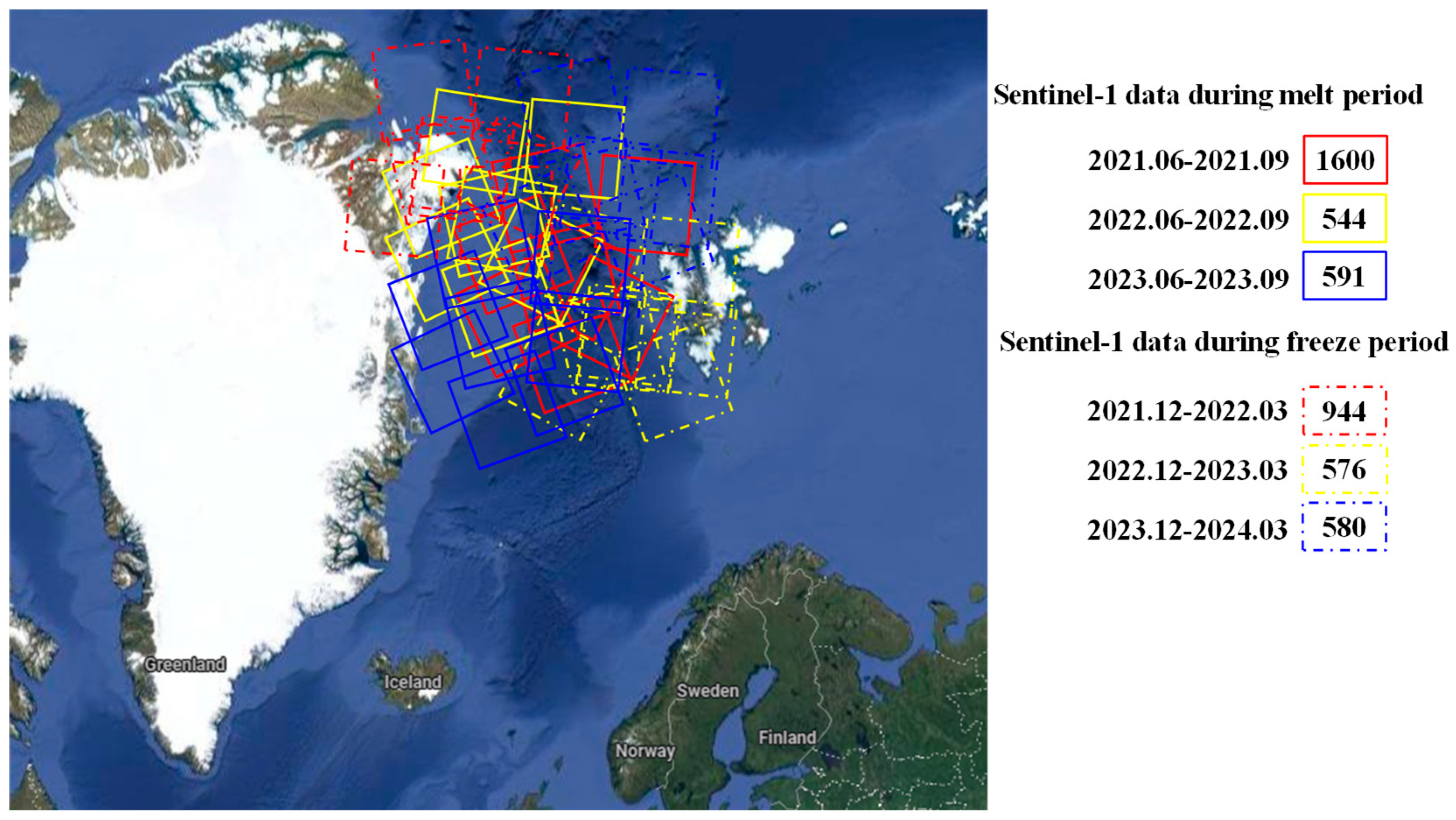
The study site for developing and testing the proposed algorithm is located in the Fram Strait region of the Arctic, covering the areas of (75°N–83°N, 15°W–15°E), see that in Figure 1. Various-scale ice floes are found in this area due to the intensive ice drift and deformation caused by the Fram Strait ice outflow (Bi et al., 2016) [23]. Sentinel-1 is a constellation of two satellites that image the entire Earth every six days. The Fram Strait is completely covered every three days using 10 Sentinel-1 EW mode dual-polarization images. In this study, the experimental data is Sentinel-1 EW mode dual-polarization data, acquired during June–September of each year from 2021 to 2023 For melt season datasets. It contains a total of 2735 images, and each image scene has a size of about 10,000 × 10,000. From December 2022 to March 2023, the winter datasets were collected with 2100 images. A whole SIC over Fram Strait with a maximum time span of 3 days (minimum of 2 days) and the overlapping areas of the images are replaced by the mean value of the backscatter in the same regions. The concerned region is generally covered only once a day when calculating the SIC. If inconsistencies in ice-water results occur on two different dates due to sea ice drift or weather effects, the classification result from the date closest in time is used for SIC retrieval (e.g., when calculating the SIC for 15 July, if there is an overlap of the 15 July and 16 July images in a certain region, the classification result of 15 July is used to express the classification result of the overlapping region and to estimate SIC).

Figure 1. The study area and details of the SAR data collection used for this research are provided. Solid rectangles represent Sentinel-1 data spanning the melt period, while dashed rectangles indicate Sentinel-1 data collected during winter.

2.2. Training and Testing Samples Dataset

2.2.1. Sample Patches for Model Training, Validating, and Testing

The cropped sample datasets have a total of 180 patches with a size of 512 × 512 (100 patches for training, 40 patches for validating, and 40 patches for testing). Each sample consists of two datasets from MET Norway ice charts and manual labeling during the melt season. Winter samples were obtained exclusively from MET Norway, without the use of manual samples. This approach was adopted primarily because there is minimal difference in training accuracy between manual samples and MET Norway samples during the melt season. Each image contains two types including sea ice and open water. The corresponding manual labels are obtained by careful visual inspection on ten original Sentinel-1 images covering the study area from 11 to 13 August 2023. A total of 140 patches for models and 100 images were randomly selected from them to train the three classifiers including the CRF, the U-Net, and the proposed Ice-WaterNet algorithm. The remaining 40 patches were used to test the validity of the models by repeating 10 times, and the output of the model parameters with the highest accuracy was used for the subsequent classification experiments. An additional 40 patches in the sample dataset were used for testing the classification models. For detailed information, please refer to Table 1.

Table 1. Sample patches for ice-water classification models training, validating, and testing.

Samples Dataset		Melt Season		Freeze Season
		MET Norway	Manual Labeling		MET Norway
Samples for Ice-WaterNet training Patch size: 512 × 512	Training	48	52	Training	48
	Validation	22	18	Validation	22
	Testing	20	20	Testing	20
	Total	90	90	Total	90

2.2.2. Image Dataset for Validating Ice–Water Classification Results

After achieving ice–water classification using the proposed model, it is necessary to validate the effectiveness of the proposed algorithm. The fair datasets for covering each whole Sentinel-1 scene have been collected. The image dataset contains a total of 800 Sentinel-1 scenes from 2021 to 2023 (Table 2). The image dataset is from the manual sea ice charts produced by the operational ice service at the Norwegian Meteorological Institute (MET Norway, https://cryo.met.no/en/latest-ice-charts (accessed on 13 October 2025)). Various data sources, including high-resolution SAR images, PM data, MODIS imagery, and AVHRR data from NOAA, are used to produce the ice charts. Each ice chart corresponding to each Sentinel-1 scene has about 10,000 × 10,000 pixels, which are assumed to represent the ground truth. The accuracies of the different algorithms for ice–water classification during the melt and freeze seasons were calculated separately.

Table 2. Samples for Ice-WaterNet results evaluation.

Freeze Season	Month
Year	December	January	February	March
2021–2022	34	35	31	34
2022–2023	34	34	31	34
2023–2024	34	34	31	34
Total	102	103	93	102
Melt Season	Month
Year	June	July	August	September
2021	34	33	34	33
2022	34	33	34	33
2023	34	33	34	31
Total	102	99	102	97

3. Methodology

3.1. Overview

The study site for developing and testing the proposed algorithm is located in the Fram Strait region of the Arctic, covering the areas of (75°N–83°N, 15°W–15°E). Various-scale ice floes are found in this area due to the intensive ice drift and deformation caused by the Fram Strait ice outflow (Bi et al., 2016) [23]. Sentinel-1 is a constellation of two satellites that image the entire Earth every six days. The Fram Strait is completely covered every three days using 10 Sentinel-1 EW mode dual-polarization images. In this study, the experimental data is Sentinel-1 EW mode dual-polarization data, acquired during June–September of each year from 2021 to 2023 For melt season datasets. It contains a total of 2735 images, and each image scene has a size of about 10,000 × 10,000. From December 2022 to March 2023, the winter datasets were collected with 2100 images. A whole SIC over Fram Strait with a maximum time span of 3 days (minimum of 2 days) and the overlapping areas of the images are replaced by the mean value of the backscatter in the same regions. The concerned region is generally covered only once a day when calculating the SIC. If inconsistencies in ice-water results occur on two different dates due to sea ice drift or weather effects, the classification result from the date closest in time is used for SIC retrieval (e.g., when calculating the SIC for 15 July, if there is an overlap of the 15 July and 16 July images in a certain region, the classification result of 15 July is used to express the classification result of the overlapping region and to estimate SIC).

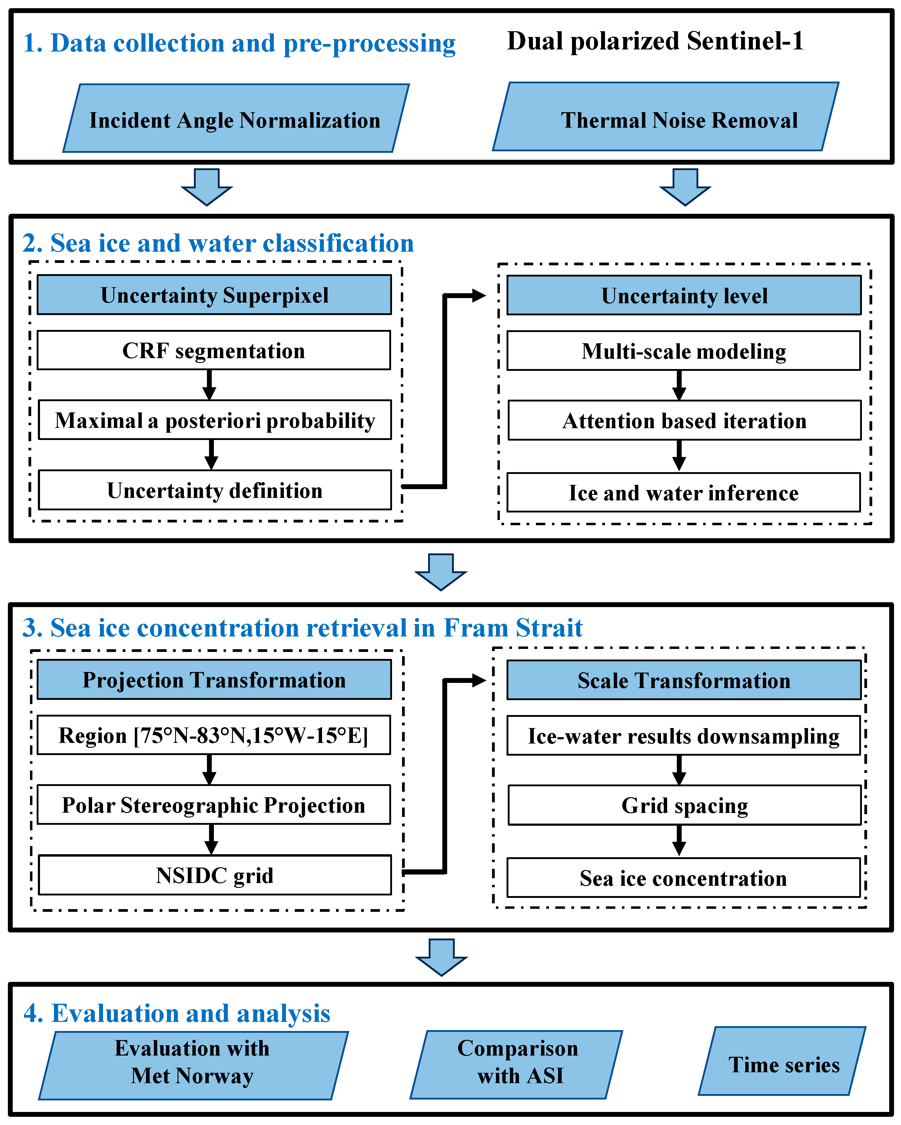
The proposed flowchart for SIC retrieval based on SAR datasets, presented in Figure 2, includes four sequential processes: (1) data collection and processing, (2) ice and water classification, (3) SIC retrieval based on the ice–water classification results, and (4) evaluation and time series analysis. The Ice-WaterNet framework, based on CRF and U-Net, is designed to identify and reduce the uncertainty of high-uncertainty superpixels, which primarily occur in thin ice, leads, and marginal ice zones during operational ice–water classification. Additionally, the framework explicitly represents multiscale floes and the diverse appearance of sea ice throughout the melt season. This study aims to reduce the uncertainty in ice–water classification to improve SIC.

Figure 2. Framework of Ice-WaterNet for SIC retrieval based on SAR datasets.

The first step of the flowchart is data collection and preprocessing is described in Section 3.2. The second step, ice–water classification, is the core methodology detailed in Section 3.3, Section 3.4 and Section 3.5. Sequential processing includes CRF and U-Net models. CRF models are used to obtain preliminary ice–water classification results at the superpixel scale and to calculate posterior probabilities to identify uncertain superpixels. The uncertainty level is ranked by comparing these results with the ice–water classification from U-Net. The third step involves retrieving SIC on NSIDC grids based on the obtained ice–water classification results, which are projected onto a polar stereographic projection NSIDC grid with a grid spacing of 1 km. The final step is evaluating the ice–water classification results and SIC products, and evaluation metrics are given in Section 3.6.

The third step involves retrieving SIC on NSIDC grids based on the obtained ice–water classification results, which are projected onto a polar stereographic projection NSIDC grid with a grid spacing of 1 km. The final step is evaluating the ice–water classification results and SIC products.

3.2. Preprocessing of Sentinel-1 Imagery

The pre-processing of the Sentinel-1 SAR dataset for this study includes the thermal noise removal and backscatter coefficients normalization. These thermal noises disrupt the SAR image, particularly in the cross-polarization channel, hindering the interpretation of forest flowers and open water. Thermal noises primarily result from the sensor system’s low signal-to-noise ratio and insufficient information about the noise vector in the EW mode. The noise tie points are provided within the metadata information in the Sentinel-1 level 1 product, and the whole noise image can be obtained from the quadratic spline interpolation in this study. After thermal noise removal, the calibrated sigma nought value of SAR backscatter is obtained using the following equation:

$${\sigma }_{cal}^0=\left(D{N}^2-noise\right)/{\left(A\right)}^2$$

(1)

where DN is Sentinel-1 image intensity from each pixel and noise is obtained from the tie points interpolation method. A is the calibration efficient and can also be obtained from the corresponding xml product files.

The backscattering intensity of open water and sea ice surfaces in SAR images varies significantly due to the incidence angle. In Sentinel-1’s extra-wide swath mode, the varying backscatter intensity across the four swaths in the entire image significantly impacts ice and water classification. As a result, the incidence angle normalization is utilized to reduce angular dependency and improve ice–water classification in this study. The normalization of incidence angles involves two key steps: the cosine approach and the calculation of the incidence angle slope (Mladenova et al., 2013) [24], as expressed by the following equation:

$${\sigma }_{ref}^0={\displaystyle \frac{{\sigma }_{cal,{\theta }_i}^0{\mathit{cos}}^n\left({\theta }_{ref}\right)}{{\mathit{cos}}^n\left({\theta }_i\right)}}$$

(2)

where $n$ is the slope, calculated as 1.99752 from the incidence angle dependent using the linear regression model; we set $n$ = 2 in this study. ${\sigma }_{cal,{\theta }_i}^0$ is the sigma nought value after the calibration of thermal noise removal. ${\theta }_i$ is the local incidence angle. The reference angle $ref$ is set to 26° based on an experiment of thousands of Sentinel-1 images (Zhang et al., 2021) [25], where the quantitative analysis was performed in intervals of 1° from 20° to 40°, and the incidence angle corresponding to the maximum coefficient of variation was selected as the reference incidence angle. After thermal noise reduction and incidence angle correction, the image’s dependence on the angle of incidence is significantly reduced, thus improving the accuracy and reliability of ice-water interpretation.

3.3. Uncertain Superpixels Segmentation Based on CRF

Hierarchical ice–water classification algorithms are presented at both pixel and superpixel scales. Pixel-level classification provides criteria for more fine-grained SIC and refines the multi-scale floes constructed based on pairwise potentials. Initially, we trained a model for ice-water segmentation using CRF, as described by the following formula:

$$P(x|y)={\displaystyle \frac{1}{Z_{CRF}}}exp\left[\sum _{i\in S}{f}_i^{unary}\left(x_i\right)+\sum _{i\in S}\sum _{j\in N_i}{f}_{ij}^{pairwise}\left(x_i,x_j|y\right)\right]$$

(3)

$$f_i^{unary}\left(x_i\right)=\sum _{i\in s}{\omega }_i\delta (y_i,l){\phi }_i\left(x_i\right)$$

(4)

$$f_{ij}^{pairwise}\left(x_i,x_j|y\right)=\sum _{i\in S}\sum _{j\in N_i}{\phi }_{i,j}(x_i,x_j|y)$$

(5)

where $Z_{CRF}$ denotes the partition function, and ${\omega }_i$ represent weight parameters of the CRF model. The unary potential $f_i^{unary}$ is defined on the individual superpixels at site $i$. $y_i$ accounts for SAR backscatter intensity in pixel $i$, and $x$ denotes its category (ice or water). $\delta (y_i,l)$ is the Dirac function, where $\delta \left(y_i,l\right)=1$ for $x_i=l$ with the ice type, and $\delta \left(y_i,l\right)=0$ for $x_i\ne l$ (open water label). The local conditional distribution $P\left(x\right|y)$ is obtained via SVM (Zhu et al., 2016) [13]. The pairwise potential $f_{ij}^{pairwise}$ describes spatial contextual information. If two classes are similar, this weight will be strengthened; conversely, if they are dissimilar, the weight will be weakened. To identify uncertain superpixels, the maximum a posteriori probability calculated from CRF models that falls between 0.15 and 0.85 is considered to indicate uncertainty. Subsequently, the uncertainty level is graded, and U-Net models are utilized to reduce this uncertainty to obtain the correct label.

3.4. Modeling the U-Net Attention Mechanism

After obtaining the uncertain superpixels from CRF, we reduce their uncertainty using the U-Net attention mechanism by re-segmenting these superpixels. The higher degree of uncertainty is primarily due to significant intraclass variances within the superpixels. Therefore, we need to re-segment these uncertain superpixels using a deep learning algorithm. To ensure each pixel receives a more definitive label, this paper uses the Binary Cross-Entropy (BCE) that constructs a superpixel loss function within a deep learning framework as follows:

$$Loss={\sum }_{i=1}^{5}BCE(M_i,GT)$$

(6)

where i represents the $i$ layer, and $GT$ denotes the ground truth. $M_i$ is updated by the attention mechanism in the channel and spatial mechanisms with respect to the Channel Attention Module and Prior Information Guide Module (PIGM) in (Li et al., 2024) [26]. The U-Net spatial attention mechanism leverages hierarchical features from the five encoders and five decoders in the encoder–decoder structure, utilizes multiscale contextual information to extract diverse ice floes, and incorporates attention modules in the decoding stage to explicitly model long-range global information. The U-Net channel attention mechanism utilizes the differences between HH and HV channels to represent sea ice and water, addressing ambiguities in ice–water classification caused by wind-roughened open water and frost flowers over leads. This approach can enhance the accuracy of ice–water classification.

In the encoder, the features for the channel and spatial mechanisms are calculated and then fused in the decoder through the cross-attention mechanism. Through each iteration, features are updated, and the highly uncertain regions are given a larger weight. The uncertainty of each pixel within the superpixels is calculated with 0.5 offset as the following equation:

$$U_{ice}^i={Sigmoid(S}_i-0.5)$$

(7)

$$U_{water}^i=Sigmoid(0.5-S_w)$$

(8)

where $U_{ice}^i$ indicates prediction uncertainty, with values near 0 showing high certainty and values near 0.5 showing high uncertainty. In each layer of the decoder, uncertainty features are combined with convolutional features from the preceding layer. This step-by-step process reduces the uncertainty of superpixels at different scales, thereby improving the final classification performance.

3.5. Base Configuration Used in the Experiment

The architecture of the U-Net-based sea ice products exists both the CRF model and the deep learning model, as depicted in Figure 3. The CRF model segments dual-polarized SAR imagery into superpixels using the meanshift method, ensuring each superpixel is no larger than 500 pixels, with a mean value offset of 0.2. The CRF model incorporates unary, pairwise, and statistical distribution potentials.

Figure 3. Illustrated architecture of the Ice-WaterNet-based sea ice products in this study.

In this study, the unary potential is derived using SVM classification, while the pairwise potential represents the connection relationship between two superpixels, with its feature function being the cross-correlation function. Additionally, a mixed statistical distribution potential, incorporating Alpha-Stable, Log-Normal, and Rayleigh distributions, is introduced. During the CRF segmentation process, the Graph Cut method based on the energy function is employed to output the posterior probabilities of the CRF. Superpixels with posterior probabilities less than 0.15 and greater than 0.85 are considered to represent stable sea water and sea ice, respectively. In contrast, superpixels with posterior probabilities between 0.15 and 0.85 are regarded as uncertain elements.

The deep learning model, U-Net, utilized dual-polarized Sentinel-1 SAR data as its input. The network architecture consists of four encoder blocks and four decoder blocks, each with three upsampling and three downsampling layers, respectively. Each encoder and decoder is connected by a convolution block, with each convolutional layer defined by a 3 × 3 kernel and a stride of 1, followed by a batch normalization and a ReLU activation function. After three distinct 1 × 1 convolution layers, the output of the final upsampling layer is the maximum a posteriori probability, which is crucial for generating sea ice uncertainty parameters. The main parameter configurations are presented in Table 1. The task performs random transformations (such as rotation and flipping) on the original 100 image samples, each sized 512 × 512, to expand the training dataset to 1200 samples. The newly generated imagery samples are then used to train the DL uncertainty model.

With a batch size of 12, a complete epoch iterates 100 times using the 1200 samples. After ten cycles of iteration, this process can reach a maximum of 1000 iterations to ensure model convergence. To further improve training efficiency, we set the iteration termination condition when the cross-entropy loss function falls below 0.005. The detailed of the parameter configuration is listed in Table 3.

Table 3. Training configuration.

Parameter	Setting
Input channel number	2
Total training epochs	10
Epoch length	20
Patch size	512
Batch size	12
Optimizer	Adam
Learning rate	0.001
Weight decay	0.0025
Scheduler	StepLR
U-Net convolution filter number	32, 64, 128, 256, 256
Data augmentation	Random Horizontal Flip Random Vertical Flip Random Rotation Random Cropping
Loss function	Cross Entropy

3.6. Evaluation Metrics

Utilizing five evaluation metrics provides a more comprehensive assessment of the effectiveness of the proposed algorithm in this study: Overall Accuracy (OA), Intersection over Union (IoU), F1-score (F1), precision, and recall. The definitions of these five evaluation metrics are as follows:

$$OA={\displaystyle \frac{\mathrm{T}\mathrm{N}+TP}{\mathrm{T}\mathrm{N}+TP+\mathrm{F}\mathrm{P}+\mathrm{F}\mathrm{N}}}$$

(9)

$$IoU={\displaystyle \frac{TP}{\mathrm{T}\mathrm{P}+\mathrm{F}\mathrm{P}+\mathrm{F}\mathrm{N}}}$$

(10)

$$Precesion={\displaystyle \frac{TP}{\mathrm{T}\mathrm{P}+\mathrm{F}\mathrm{P}}}$$

(11)

$$Recall={\displaystyle \frac{TP}{\mathrm{T}\mathrm{P}+\mathrm{F}\mathrm{N}}}$$

(12)

$$F1={\displaystyle \frac{2\times Precision\times Recall}{Precision+Recall}}$$

(13)

where true negatives, true positives, false positives, and false negatives are denoted as TN, TP, FP, and FN, respectively. These four metrics, including IoU, precision, recall, and F1-score, are used to assess the proposed algorithm’s performance for ice–water classification.

4. Results and Discussion

To evaluate the performance of the proposed Ice-WaterNet algorithm in this study, we utilized two datasets: one covering the melt season from June to September and another for the winter season from December to March. These datasets comprised 4835 Sentinel-1 images. The assessment was based on both visual inspection and quantitative evaluation. To ensure a comprehensive and fair comparison, we selected the CRF and U-Net models as state-of-the-art (SOTA) algorithms. The performance of the CRF, U-Net, and Ice-WaterNet algorithms was assessed using datasets from 2021 to 2023, encompassing both the melt and freeze seasons, for both quantitative and visual comparison.

4.1. Experimental Results Quantitative Comparison During Melt Season and Freeze Season

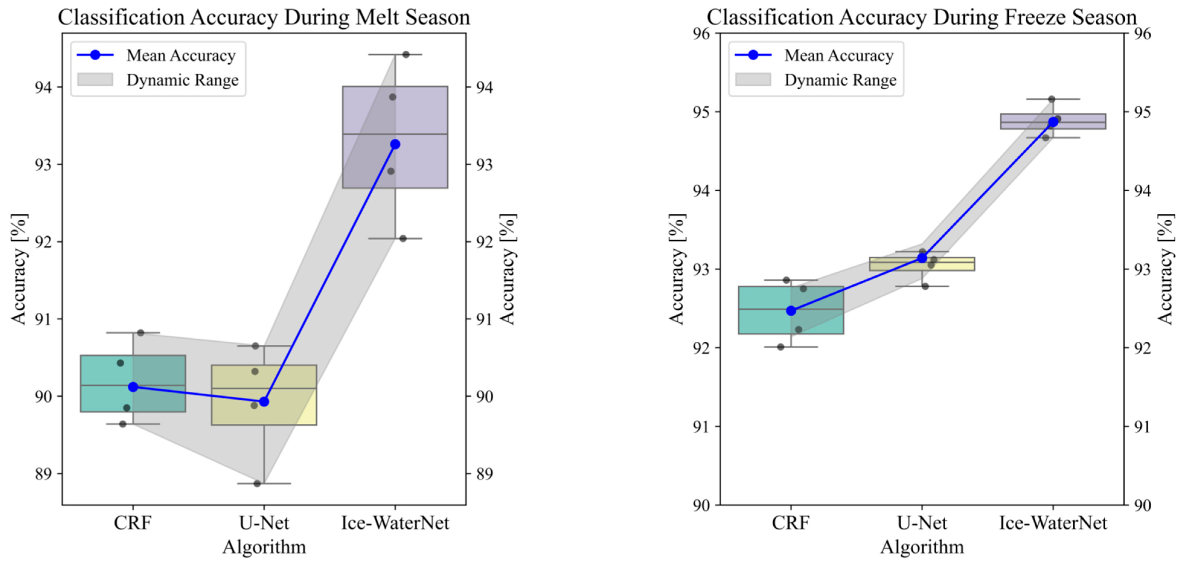
To compare the performance of different algorithms across seasons, the proposed Ice-WaterNet algorithm and SOTA methods were applied to datasets from both the melt and freeze seasons. Overall Accuracy (OA) was used to evaluate performance, as shown in Figure 4. Ice-WaterNet achieved the highest OA during both the melt and winter seasons. Among the algorithms, the CRF method performed best during the melt season, while U-Net performed the worst. This discrepancy can be attributed to the ambiguity caused by wet snow or melt ponds, which significantly reduce SAR backscatter coefficients. In the marginal sea ice zone (MIZ), the effects of winds and ocean currents on SAR backscatter can create further ambiguities between ice and water. Conversely, under calm conditions, the contrast between thin ice and flat open water diminishes, reducing the separability of level ice. The melt season poses the greatest challenge for reliable ice–water classification. However, Ice-WaterNet robustly outperformed the other methods during the winter season in terms of OA. Overall, the proposed Ice-WaterNet algorithm demonstrated superior performance over the two SOTA methods, regardless of the season.

Figure 4. Visual comparison on datasets across different seasons.

In addition to OA, four additional metrics—IoU, Precision, Recall, and F1—were calculated, as presented in Table 4, which lists the monthly performance of the different methods on the two datasets. Compared to other SOTA methods, our proposed Ice-WaterNet achieved the best performance across all metrics. The analysis reveals that Ice-WaterNet performs optimally during the transitional periods in September and March, coinciding with the maximum and minimum ice extents. In summer, the Ice-WaterNet outperforms the SOTA method CRF by 3.375% on the IoU metric, 2.83% on the precision metric, 3.3375% on the recall metric, and 3.09% on the F1 metric. In Winter, the Ice-WaterNet outperforms the SOTA method CRF by 1.9625% on the IoU metric, 2.1% on the precision metric,1.8875% on the recall metric, and 1.745% on the F1 metric. Due to the dynamic changes during the melt season, ice–water classification presents significant challenges. The algorithm proposed in this study not only enhances the accuracy of ice–water classification during the winter season but also substantially improves accuracy during the summer season. It can be stated that our Ice-WaterNet algorithm outperforms SOTA algorithms across all evaluation metrics.

Table 4. Comparison of melt season and freeze season sample dataset performance on datasets for each month during the melt season and the freeze season. For each metric, the best scores are marked in red and sub-optimal scores are underlined.

Month	CRF				U-Net				Ice-WaterNet
	IoU	Precision	Recall	F1	IoU	Precision	Recall	F1	IoU	Precision	Recall	F1
June	85.82	91.02	91.52	91.26	84.88	90.88	90.04	90.46	88.12	93.14	93.24	93.19
July	84.85	90.85	90.31	90.57	83.95	90.87	89.62	90.24	87.91	93.31	93.87	93.59
August	84.32	90.64	90.64	90.64	85.65	91.25	90.23	90.74	88.87	93.89	94.52	94.20
September	85.43	90.23	90.73	90.47	85.32	91.42	90.62	91.02	89.02	93.72	94.92	94.32
December	88.43	92.71	93.81	93.26	89.91	93.98	93.68	93.83	90.56	94.66	95.24	94.95
January	88.73	92.63	93.63	93.13	88.76	94.12	93.72	93.92	90.21	95.31	95.37	94.34
February	88.16	93.41	93.26	93.33	88.85	93.85	94.05	93.95	90.33	95.47	95.47	95.47
March	88.35	93.55	93.45	93.50	88.92	93.72	93.88	93.90	90.42	95.26	95.62	95.44

In addition, the average processing time for a single Sentinel-1 scene (approximately 10,000 × 10,000 pixels) was around 12 min on a standard GPU (NVIDIA RTX 3090), which is feasible for operational use given the bi-daily update cycle of SIC products. For comparison, standalone U-Net required ~10 min, while CRF alone took ~7.5 min per scene. Although Ice-WaterNet incurs additional time due to uncertainty refinement, the analysis presented in Figure 1 demonstrates that generating daily sea ice concentration products takes less than two hours. This timeframe remains acceptable for operational monitoring requirements, while the model’s superior accuracy justifies the trade-off.

4.2. Visual Performance Comparison of Ice–Water Classification Results

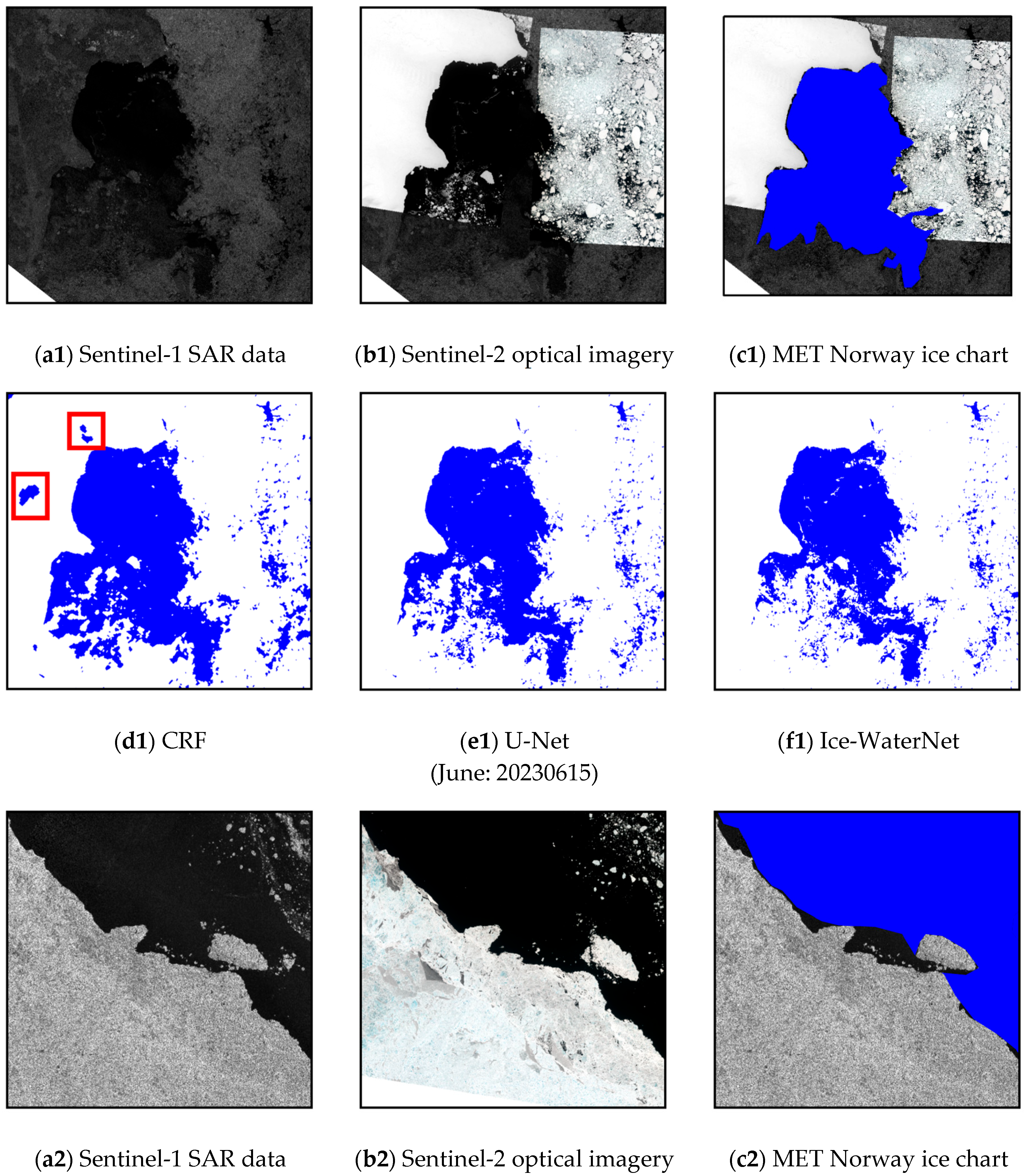
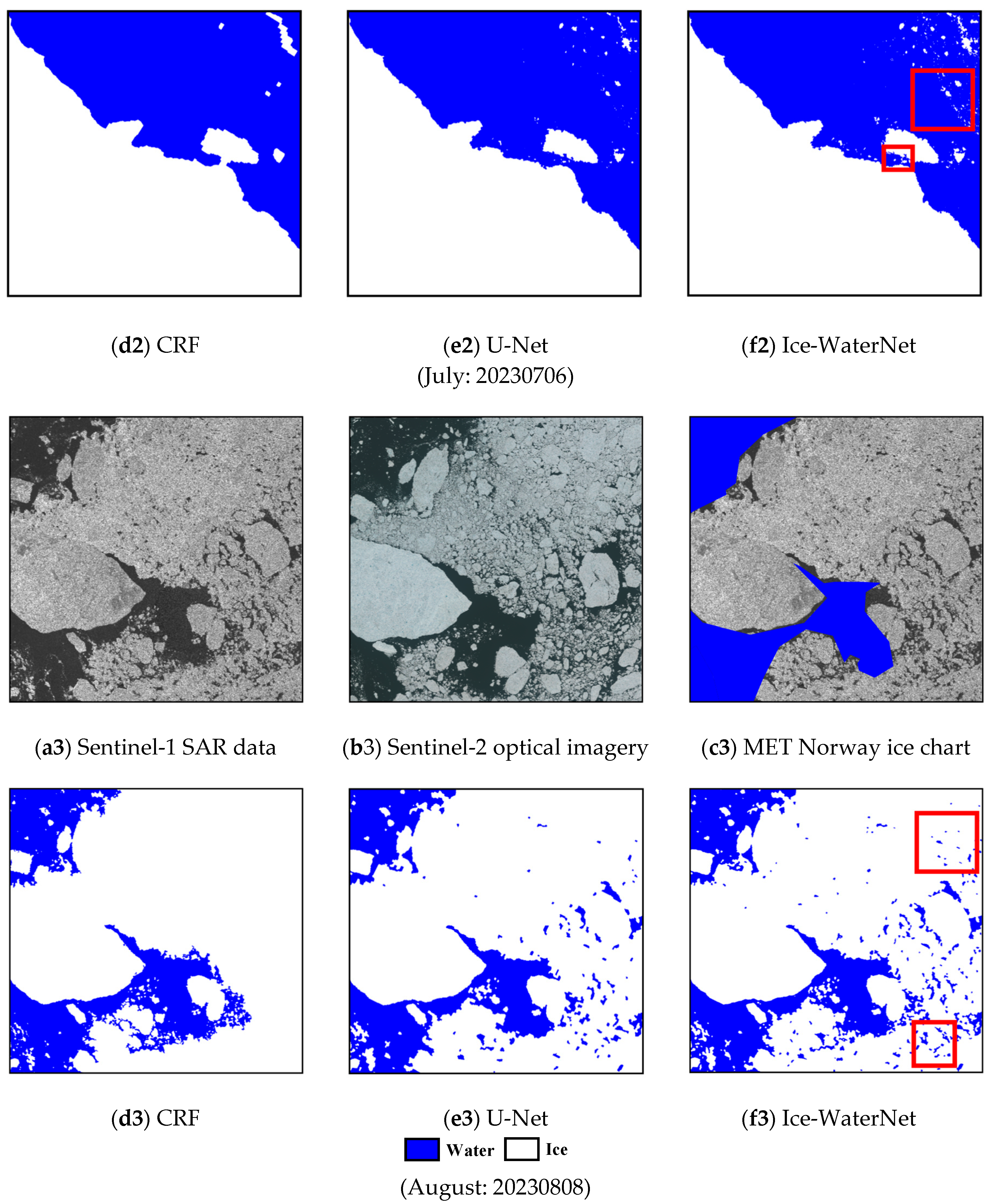
SAR scenes obtained during the melt and freeze-up periods are particularly challenging for sea ice mapping due to factors such as melt ponds, thin ice, and wind-roughened water. To provide a more intuitive comparison of our Ice-WaterNet algorithm with SOTA methods, we visualized the extraction results of all methods and compared them with optical imagery and the MET Norway Ice charts. The visualization of the experimental results in Figure 5 demonstrates that the proposed algorithm effectively reduces or eliminates inconsistencies at the open water boundary. When combined with optical Sentinel-2 imagery and MET Norway Ice charts, our algorithm, along with CRF and U-Net, delivers fine water boundaries from the ice–water classification results. For instance, in the June example scene (Figure 5(e1)), the CRF method misclassified ice as open water due to the low intensity of level ice in the upper left region. The U-Net method performed slightly better than the CRF method. However, from a visual assessment perspective, the proposed algorithm provides the most detailed ice–water classification results. As illustrated in the July example scene (Figure 5(f2)), CRF and U-Net were unable to detect the presence of icebergs, while Ice-WaterNet performed slightly better. In the August example scene (Figure 5(f3)), our Ice-WaterNet accurately extracted small ponds appearing on the ice surface during the melt season, closely matching the optical imagery. Although all comparison methods missed the small icebergs highlighted in the red circle, our Ice-WaterNet demonstrated its superiority. Overall, all methods effectively delineate the ice-water boundary, particularly the proposed algorithm, which successfully mitigates the backscattering coefficient variations caused by wind and ocean currents.

Figure 5. Visual comparison of the dataset during the melt season. (a) The original Sentinel-1 HH image. (b) The optical Sentinel-2 imagery. (c) The MET Norway ice charts. (d) The CRF classification result. (e) The U-Net classification result. (f) The Ice-WaterNet classification result. The red pixels are misclassified (the case where the classification result is inconsistent with the ground truth).

4.3. Ice–Water Classification Results and SIC on Each Sentinel-1 Scene Data

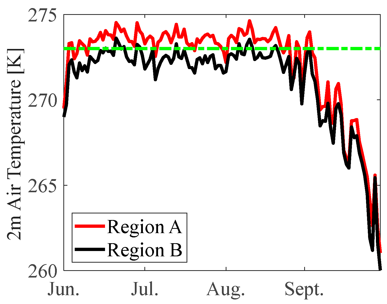
For the proposed method to be useful for SIC retrieval, the Ice-WaterNet model must be developed to produce the SIC and compared with the classical and widely used SIC products. In addition to the SOTA algorithm, we also selected ASI as the comparison. The example scenes were selected from the melt season over each month given in Figure 6. In the first row of sample images, a large area of open water is observed. Due to the limitations of data spatial resolution, the ASI concentration product overestimates the open water area (indicated by the yellow region in the image). In contrast, the other three methods based on Sentinel-1 data accurately identify the open water area. We compared the surface temperatures (Figure 7) of the black open water and the red sea ice regions, as shown in the figure below. The yellow area, with a temperature of 274.86 K (approximately 1.7 °C), indicates the absence of sea ice in that region.

Figure 6. Sentinel-1 ice–water classification results. Pixel-level SIC retrieval during the melt period in Fram Strait, Arctic. From the first row to the fourth row, the dates are 15 June 2023, 6 July 2023, 8 August 2023, and 25 September 2023, respectively. The marked area A and B in column 3, row 1 represents the sample area, and the corresponding daily temperature of these two areas are given in Figure 7.

Figure 7. The 2 m air temperature from ERA5 for Region A and Region B, where Region A represents open water and Region B represents sea ice. The ERA5 reanalysis datasets were downloaded from the Copernicus data portal at: https://cds.climate.copernicus.eu/#!/home (accessed on 13 October 2025), the green line it the frozen line with the temperature of 273 K.

As sea ice melts, Sentinel-2 imagery data from 6 July indicate that the ASI data underestimates the concentration of large floating ice in the open water areas (as shown in the black region of the image). Compared to the superpixel-level CRF algorithm, U-Net and Ice-WaterNet, through the construction of multi-scale networks, not only accurately distinguish between open water and sea ice but also precisely identify melting ponds or varied size floes. Similarly, for the ice-water edge regions in the 20230808 data, the ASI product provides only a blurred boundary, whereas the sea ice concentration results based on high-resolution Sentinel-1 data offer a more detailed delineation. Compared to the U-Net network, Ice-WaterNet introduces the concept of uncertainty levels, which enhances the description of sea ice features across different scales through feature optimization and iterative processes between layers. By September, as sea ice aggregates and grows, there are often large areas of relatively small open water and thin ice-covered regions within high concentration ice zones. The ASI product fails to capture this information, resulting in an overestimation of ice concentration.

4.4. Time Series Analysis of SIC in Fram Strait

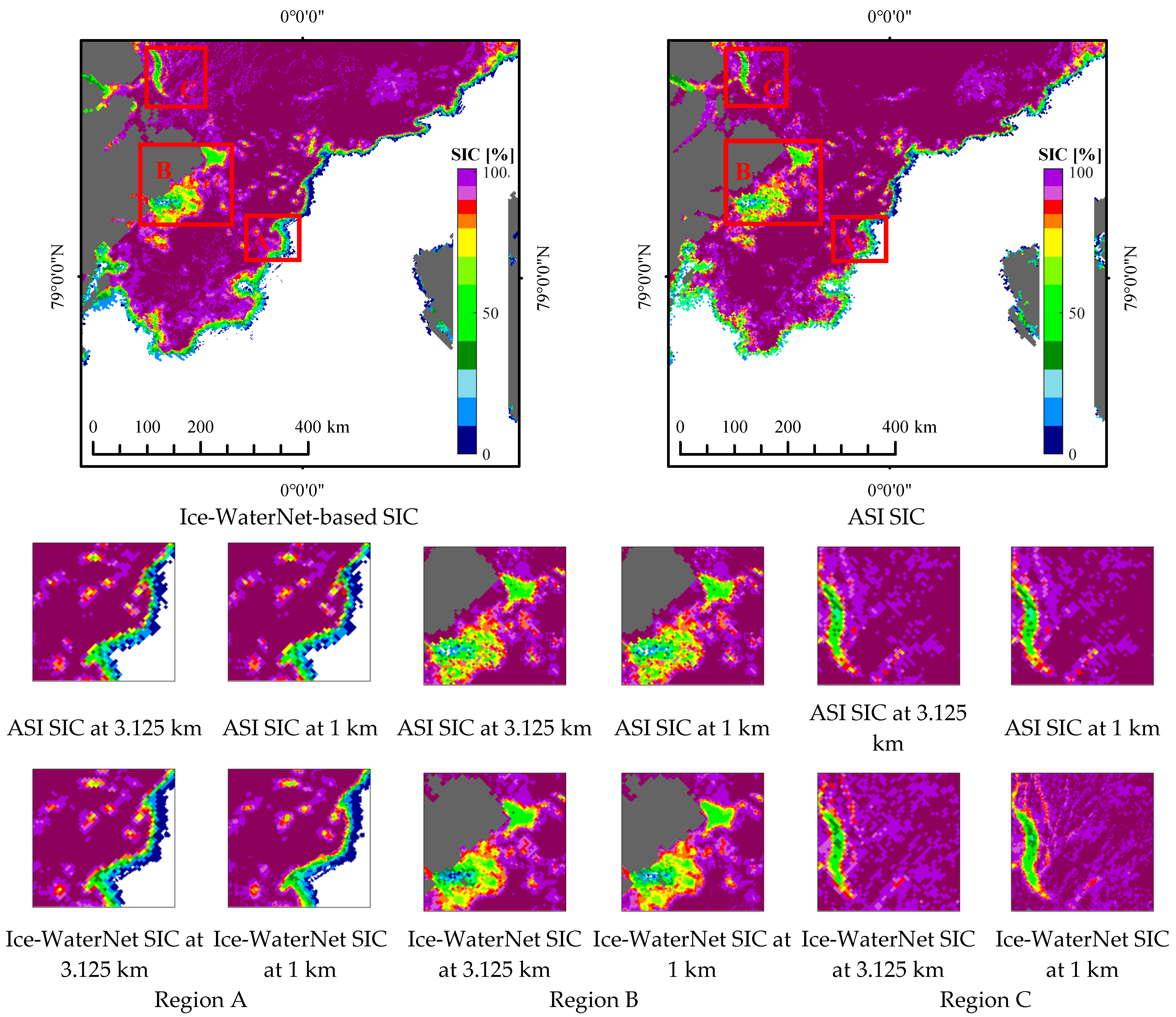
Different sea ice concentration (SIC) products for 30 September 2023 from the ASI and our proposed algorithm in the Fram Strait are visually compared in Figure 8. The SIC results of the two algorithms generally coincide, with the main deviations occurring in the sea ice marginal regions and leads. Our proposed algorithm appears more detailed and provides clearer boundaries between ice and water. Overall, the Ice-WaterNet concentration exhibits richer texture features compared to the ASI sea ice concentration, offering more detailed characteristics. For Region A, located in the sea ice marginal area, Ice-WaterNet identifies more sea ice details and provides a clearer ice edge line. In Region B, situated in a polynya area, Ice-WaterNet and ASI results are similar for high-concentration areas outside the polynya. However, within the low-concentration areas of the polynya, Ice-WaterNet provides more refined details. In Region C, corresponding to a lead area, Ice-WaterNet demonstrates clearer edge lines and more pronounced linear features around the leads.

Figure 8. SIC retrieval from Sentinel-1 ice–water classification results in Fram Strait: 30 September 2023.

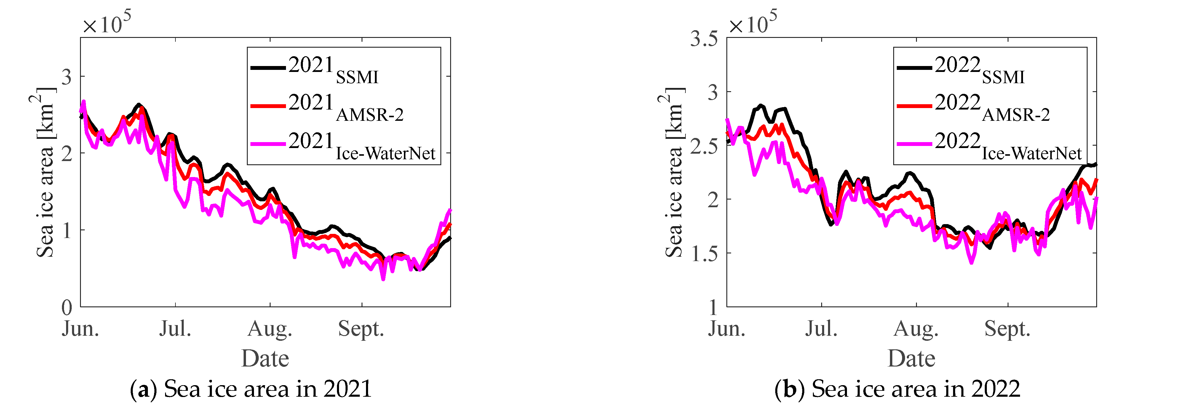
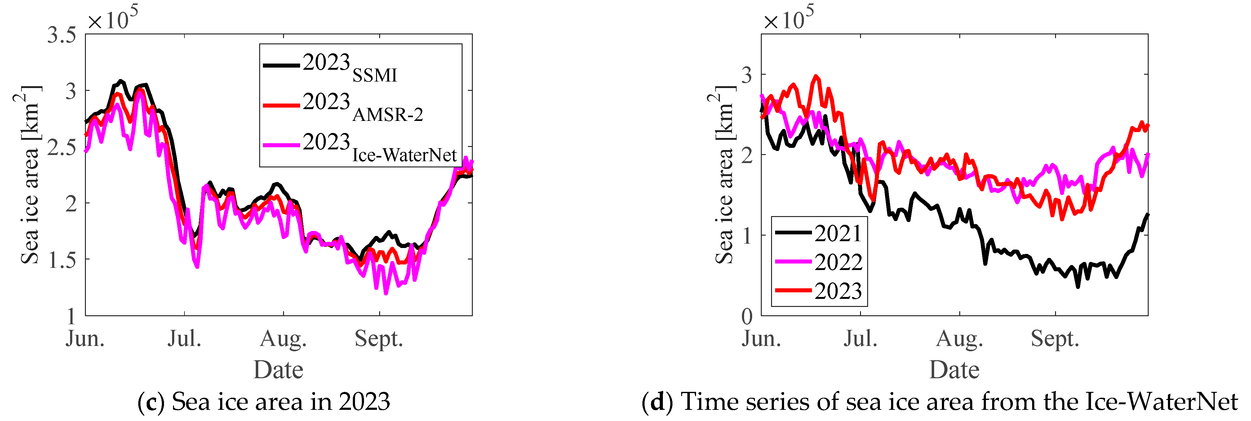
Figure 9 shows the sea ice area calculated using SIC from 2021 to 2023 in the Fram Strait, Arctic. The interannual variation in sea ice area is consistent, except during the early melting period (early June) and the early freezing period (late September). During these times, the sea ice area follows the pattern of SSM/I > AMSR-2 > Sentinel-1. This pattern is very clear in 2021, shows more fluctuations in 2022, and in 2023, the differences among the three data sources are relatively small. Overall, the trend indicates that passive microwave retrievals tend to overestimate sea ice area, while high-resolution SAR-based active microwave algorithms provide more accurate SIC products. These SAR-based results reflect sea ice changes more precisely, suggesting that the extent of sea ice melt is more severe than previously estimated.

Figure 9. Sea ice area in Fram Strait from 2021 to 2023. Three figures represent the sea ice area for 2021, 2022, and 2023. The red line indicates the results from SSM/I (12.5 km resolution), the purple line shows the results from AMSR (3.125 km resolution), and the black line represents the results from Sentinel-1 (40 m resolution).

5. Conclusions

High-resolution SAR-based active microwave algorithms offer significant advantages in sea ice classification and monitoring. Compared to PM based SIC retrievals, high-resolution SAR data provides more accurate products, allowing SIC for a more precise reflection of sea ice area trends. The rich texture features and detailed characteristics captured by SAR data not only result in clearer sea ice and water boundaries but also reveal that the extent of sea ice melt is more severe than previously estimated. In this article, we argue that the complex distribution of the sea ice, inconsistent backscatter coefficients, and various floe sizes bring some uncertainty to the predictions of the general deep learning models, causing the omission and the commission to a large extent. Therefore, we introduce the concept of uncertainty and propose a novel Ice-WaterNet by combining the ML and DL algorithm. First, we utilize the CRF model to generate the uncertain superpixels for ice–water classification. Second, we propose the dual attention mechanism-based U-Net deep learning models to enhance the highest-level features and eliminate the uncertainty of features from high level to low level. Finally, the accurate ice–water classification results are used to produce SIC products. By conducting sufficient experiments, we validate the effectiveness of the proposed Ice-WaterNet on ice–water classification task by comparing it with CRF and U-Net using three years of Sentinel-1 datasets in the Fram Strait. Traditional algorithms are significantly affected by seasonal variations, showing considerable performance differences between summer and winter datasets. The Ice-WaterNet algorithm proposed in this study effectively mitigates the impact of these seasonal variations, resulting in highly accurate ice–water classification results. The final SIC products have also been used to calculate sea ice area for interannual and intra-annual variations and trend analysis. The final high accuracy on ice–water classification results and high spatial resolution SIC products are compared with the SOTA algorithm and ASI, indicating that the proposed Ice-WaterNet has superiority over other methods. The proposed Ice-WaterNet not only enhances PM SIC retrievals by providing high spatial resolution training data but also advances ice–water classification algorithms across various scenarios. This progress could lead to new insights into sea ice classification methodologies during the melt season. Furthermore, the performance of the Ice-WaterNet model for SIC retrieval for the whole Arctic remains an important and promising direction for future research.

References

- Asadi, N.; Scott, K.A.; Komarov, A.S.; Buehner, M.; Clausi, D.A. Evaluation of a Neural Network with Uncertainty for Detection of Ice and Water in SAR Imagery. IEEE Trans. Geosci. Remote Sens. 2021, 59, 247–259. [Google Scholar] [CrossRef]
- Chen, X.; Cantu, F.J.P.; Patel, M.; Xu, L.; Brubacher, N.C.; Scott, K.A.; Clausi, D.A. A comparative study of data input selection for deep learning-based automated sea ice mapping. Int. J. Appl. Earth Obs. Geoinf. 2024, 131, 103920. [Google Scholar] [CrossRef]
- Wu, A.; Che, T.; Li, X.; Zhu, X. Routeview: An intelligent route planning system for ships sailing through Arctic ice zones based on big Earth data. Int. J. Digit. Earth 2022, 15, 1588–1613. [Google Scholar] [CrossRef]
- Huang, Z.; Yao, X.; Liu, Y.; Dumitru, C.O.; Datcu, M.; Han, J. Physically explainable CNN for SAR image classification. ISPRS J. Photogramm. Remote Sens. 2022, 190, 25–37. [Google Scholar] [CrossRef]
- Ivanova, N.; Pedersen, L.T.; Tonboe, R.T.; Kern, S.; Heygster, G.; Lavergne, T.; Sørensen, A.; Saldo, R.; Dybkjær, G.; Brucker, L.; et al. Inter-comparison and evaluation of sea ice algorithms: Towards further identification of challenges and optimal approach using passive microwave observations. Cryosphere 2015, 9, 1797–1817. [Google Scholar] [CrossRef]
- Chi, J.; Kim, H.C.; Lee, S.; Crawford, M.M. Deep learning based retrieval algorithm for Arctic sea ice concentration from AMSR2 passive microwave and MODIS optical data. Remote Sens. Environ. 2019, 231, 111204. [Google Scholar] [CrossRef]
- Jiang, L.; Chen, F.; Yu, D.; Ma, Y.; Zhao, D.; An, D. Automatic High-Accuracy Sea Ice Monitoring in the Arctic Using MODIS Data. IEEE Trans. Geosci. Remote Sens. 2023, 61, 4301413. [Google Scholar] [CrossRef]
- Li, X.; Xiong, C. Estimating Sea Ice Concentration from Microwave Radiometric Data for Arctic Summer Conditions using Machine Learning. IEEE Trans. Geosci. Remote Sens. 2024, 62, 4301018. [Google Scholar] [CrossRef]
- Cooke, C.L.V.; Scott, K.A. Estimating Sea Ice Concentration from SAR: Training Convolutional Neural Networks with Passive Microwave Data. IEEE Trans. Geosci. Remote Sens. 2019, 57, 4735–4747. [Google Scholar] [CrossRef]
- Karvonen, J. Baltic sea ice concentration estimation based on C-band HH-polarized SAR data. IEEE J. Sel. Top. Appl. Earth Obs. Remote Sens. 2012, 5, 1874–1884. [Google Scholar] [CrossRef]
- Karvonen, J. Baltic Sea Ice Concentration Estimation from C-Band Dual-Polarized SAR Imagery by Image Segmentation and Convolutional Neural Networks. IEEE Trans. Geosci. Remote Sens. 2021, 60, 4301411. [Google Scholar] [CrossRef]
- Huang, L.; Qiu, Y.; Li, Y.; Yu, S.; Zhong, W.; Dou, C. DynIceData: A gridded ice–water classification dataset at short-time intervals based on observations from multiple satellites over the marginal ice zone. Big Earth Data 2023, 8, 249–273. [Google Scholar] [CrossRef]
- Zhu, T.; Li, F.; Heygster, G.; Zhang, S. Antarctic Sea-Ice Classification Based on Conditional Random Fields from RADARSAT-2 Dual-Polarization Satellite Images. IEEE J. Sel. Top. Appl. Earth Obs. Remote Sens. 2016, 9, 2451–2467. [Google Scholar] [CrossRef]
- Khaleghian, S.; Ullah, H.; Kraemer, T.; Eltoft, T.; Marinoni, A. Deep Semisupervised Teacher-Student Model Based on Label Propagation for Sea Ice Classification. IEEE J. Sel. Top. Appl. Earth Obs. Remote Sens. 2021, 14, 10761–10772. [Google Scholar] [CrossRef]
- Wang, L.; Scott, K.A.; Clausi, D.A. Sea ice concentration estimation during freeze-up from SAR imagery using a convolutional neural network. Remote Sens. 2017, 9, 408. [Google Scholar] [CrossRef]
- Ren, Y.; Li, X.; Yang, X.; Xu, H. Development of a Dual-Attention U-Net Model for Sea Ice and Open Water Classification on SAR Images. IEEE Geosci. Remote Sens. Lett. 2022, 19, 4010205. [Google Scholar] [CrossRef]
- Wang, Q.; Lohse, J.P.; Doulgeris, A.P.; Eltoft, T. Data Augmentation for SAR Sea Ice and Water Classification Based on Per-Class Backscatter Variation with Incidence Angle. IEEE Trans. Geosci. Remote Sens. 2023, 61, 4205915. [Google Scholar] [CrossRef]
- Mahmud, M.S.; Nandan, V.; Singha, S.; Howell, S.E.L.; Geldsetzer, T.; Yackel, J.; Montpetit, B. C- and L-band SAR signatures of Arctic sea ice during freeze-up. Remote Sens. Environ. 2022, 279, 113129. [Google Scholar] [CrossRef]
- Zhang, T.; Yang, Y.; Shokr, M.; Mi, C.; Li, X.M.; Cheng, X.; Hui, F. Deep learning based sea ice classification with gaofen-3 fully polarimetric sar data. Remote Sens. 2021, 13, 1452. [Google Scholar] [CrossRef]
- Zhao, L.; Xie, T.; Perrie, W.; Yang, J. Deep-Learning-Based Sea Ice Classification with Sentinel-1 and AMSR-2 Data. IEEE J. Sel. Top. Appl. Earth Obs. Remote Sens. 2023, 16, 5514–5525. [Google Scholar] [CrossRef]
- Huang, R.; Wang, C.; Li, J.; Sui, Y. DF-UHRNet: A Modified CNN-Based Deep Learning Method for Automatic Sea Ice Classification from Sentinel-1A/B SAR Images. Remote Sens. 2023, 15, 2448. [Google Scholar] [CrossRef]
- Park, J.W.; Korosov, A.A.; Babiker, M.; Won, J.S.; Hansen, M.W.; Kim, H.C. Classification of sea ice types in Sentinel-1 synthetic aperture radar images. Cryosphere 2020, 14, 2629–2645. [Google Scholar] [CrossRef]
- Bi, H.; Sun, K.; Zhou, X.; Huang, H.; Xu, X. Arctic Sea Ice Area Export Through the Fram Strait Estimated from Satellite-Based Data: 1988–2012. IEEE J. Sel. Top. Appl. Earth Obs. Remote Sens. 2016, 9, 3144–3157. [Google Scholar] [CrossRef]
- Mladenova, I.E.; Jackson, T.J.; Bindlish, R.; Hensley, S. Incidence angle normalization of radar backscatter data. IEEE Trans. Geosci. Remote Sens. 2013, 51, 1791–1804. [Google Scholar] [CrossRef]
- Zhang, Y.; Zhu, T.; Spreen, G.; Melsheimer, C.; Huntemann, M.; Hughes, N.; Zhang, S.; Li, F. Sea ice and water classification on dual-polarized Sentinel-1 imagery during melting season. Cryosphere Discuss. 2021, 2021, 1–26. [Google Scholar]
- Li, J.; He, W.; Cao, W.; Zhang, L.; Zhang, H. UANet: An Uncertainty-Aware Network for Building Extraction from Remote Sensing Images. IEEE Trans. Geosci. Remote Sens. 2024, 62, 5608513. [Google Scholar] [CrossRef]
Disclaimer/Publisher’s Note: The statements, opinions and data contained in all publications are solely those of the individual author(s) and contributor(s) and not of MDPI and/or the editor(s). MDPI and/or the editor(s) disclaim responsibility for any injury to people or property resulting from any ideas, methods, instructions or products referred to in the content. |
© 2025 by the authors. Licensee MDPI, Basel, Switzerland. This article is an open access article distributed under the terms and conditions of the Creative Commons Attribution (CC BY) license (https://creativecommons.org/licenses/by/4.0/).