Article

Flood Susceptibility Mapping Using Machine Learning and Geospatial-Sentinel-1 SAR Integration for Enhanced Early Warning Systems

1
Department of Civil and Environmental Engineering, Lamar University, Beaumont, TX 77710, USA
2
Department of Industrial and Systems Engineering, Lamar University, Beaumont, TX 77710, USA
*
Author to whom correspondence should be addressed.
Remote Sens. 2025, 17(20), 3471; https://doi.org/10.3390/rs17203471
Submission received: 13 August 2025 / Revised: 8 October 2025 / Accepted: 13 October 2025 / Published: 17 October 2025

Abstract

Highlights

What are the main findings?
  • A multi-year flood inventory was generated from Sentinel-1 SAR imagery (2018–2023) using Google Earth Engine, capturing repeated ponding occurrences as inputs for the target of susceptibility modeling.
  • Flood susceptibility maps were developed using both a statistical model (FR) and machine learning models (RF, XGBoost, CNN), with model performance assessed through AUC and feature interpretability evaluated with SHAP and validated with available high-risk locations monitored by early warning flood sensors.
What is the implication of the main finding?
  • The integration of SAR-based flood inventory with geospatial factors provides a robust framework for identifying high-frequency flood-prone areas in Jefferson County, TX, serving as a representative example for data-scarce regions.
  • The methodology supports data-driven flood risk management by offering accurate, interpretable, and transferable tools that can inform planning and adaptation strategies in other flood-prone regions.

Abstract

This study presents a comprehensive framework for flood susceptibility mapping by integrating geospatial factors with both statistical and machine learning models. Thirteen Flood-related factors, including DEM, slope, TWI, NDVI, etc., are extracted as features of models, and historical flood data derived from Sentinel-1 SAR from 2018 to 2023 are used as the target variables of the models. These datasets are analyzed using a frequency-based statistical model and three machine learning models, including Random Forest, XGBoost, and CNN, to generate flood susceptibility maps. The performance of each model is evaluated through AUC; and SHAP scores are separately generated for Machine learning (ML) models to explain each feature contribution in the ML model. The generated susceptibility maps are validated by high-flood-risk locations monitored by flood sensors, BLE inundation models, and flood-prone areas suggested by the Local Community Task Force. The results indicate that the XGBoost model outperforms all other models, with an AUC of 0.92 and demonstrates the highest alignment with recommended high-flood-risk locations, while the frequency-based statistical model showed the weakest performance with an AUC of 0.65. SHAP value graphs highlight the elevation, slope, and TWI as the most influential features across all models. The susceptibility maps generated by the machine learning model show strong agreement with the BLE map and high-flood-risk areas identified by the local Community Task Force.

1. Introduction

Floods are natural events that regularly occur in the United States, including hurricanes and tornadoes, on small and regional scales, which the country experiences every year [1,2,3,4,5]. According to the Federal Emergency Management Agency (FEMA), flooding ranks as the foremost natural hazard in the United States [6]. Furthermore, the National Weather Service (NWS) reports that after heat waves, floods are the second leading cause of weather-related fatalities in the United States [7].
Over the last 50 years, thousands of flood events have been recorded, since 1975, and an average of 125 deaths annually, totaling roughly 5000–6000 fatalities nationwide, plus several thousand injuries (e.g., 146 deaths and 60 injuries in 2021 alone). Texas is the nation’s most flood-prone state, enduring hundreds of floods and over 70 major federal flood disasters since 1975; it also leads the country in fatalities, with an estimated 800+ deaths over the past 50 years and likely hundreds of injuries [8,9]. Southeast Texas, especially Jefferson County, is among the hardest-hit areas due to tropical storms and Gulf rainfall, suffering dozens of flood-related deaths over recent decades. Catastrophic events such as Hurricane Harvey (2017), which dumped a U.S. record 60.58 inches of rain in Jefferson County and caused 68 deaths statewide, and Tropical Storm Imelda (2019), which killed 5 people (3 in Jefferson County) and forced hundreds of rescues, highlight the extreme vulnerability of this region to deadly and destructive flooding [10,11].
The National Hurricane Center (NHC) officially recognized Hurricane Harvey as the most significant tropical cyclone rainfall event in U.S. history and the second most destructive hurricane, after Hurricane Katrina, in terms of losses [12,13]. This powerful storm impacted Southeast Texas from late August to September 2017, resulting in the recorded accumulation of over 60 inches of rainfall in the vicinity of Nederland and Groves, Texas [14]. Two years after Hurricane Harvey, Tropical Storm Imelda happened in Southeast Texas in September 2019, marking the fourth time in a decade that flooding closed Interstate I-10. In order to improve cooperation in handling the region’s regular floods, the Southeast Texas Flood Coordination Study (SETxFCS) was established in November 2019. The Flood Coordination Study project involves managing over 80 low-cost flood sensors across seven counties in coordination with DHS S&T. Tasks include installation support, asset management, elevation mapping, and establishing alert thresholds to enhance data visualization on OneRain platforms [15,16].
Flood Susceptibility Mapping is crucial for mitigating flood hazards by identifying vulnerable areas using Remote Sensing (RS) and Geographic Information System (GIS) tools. The increasing frequency and intensity of floods, driven by climate change and land-use changes, emphasize the need for effective flood susceptibility assessments. In this paper, the term flood susceptibility refers to all areas where water ponding has occurred. While ponding susceptibility may be a more precise term for this context, since the target values used in all modeling are water pixel data derived from Sentinel-1 SAR imagery, the broader and more widely accepted term flood susceptibility is used for clarity and general applicability. Flood susceptibility is determined by various physical factors such as digital elevation model (DEM), slope, soil type, land use/land cover (LULC), topographic wetness index (TWI), etc. The selection of these conditioning factors depends on the spatial scale of the study. Large-scale analyses use fewer factors for consistency, whereas local-scale studies incorporate more location-specific data for accuracy. Geographic Information Systems (GIS) play a key role in integrating these factors to create flood susceptibility maps [17,18,19,20,21,22].
Flood Susceptibility Mapping methodologies can be categorized into three main groups:
Hydrological Methods: Hydrological methods for flood susceptibility mapping include models like SWAT, WetSpa, and HYDROTEL, which simulate flood events by analyzing water flow dynamics and considering factors such as land use, soil type, topography, and climate data. These approaches are powerful as they capture complex rainfall–runoff interactions, integrate with climate change models, and can be combined with decision-making tools like AHP or TOPSIS to generate robust flood zoning maps. However, they also have weaknesses, including high data demands, reduced accuracy at small or local scales, and uncertainties in downscaling climate models such as GCMs, which limit their reliability in data-scarce regions [23,24].
Statistical and Knowledge-Based Methods: Approaches such as Weights of Evidence (WoE), Logistic Regression (LR), Frequency Ratio (FR), and Analytic Hierarchy Process (AHP) are commonly used in GIS to assess flood susceptibility based on conditioning factors. Multi-Criteria Decision Analysis (MCDA), particularly AHP, integrates socio-economic and environmental indicators for decision-making but faces limitations in handling uncertainties and nonlinear dynamics. These complexities are better addressed using physical models or advanced machine learning techniques, though they require extensive data, computational resources, and expert knowledge [25,26].
Machine Learning Methods: Machine learning (ML) methods have emerged as a reliable and objective approach for flood susceptibility and risk assessment, especially under the growing pressures of rapid urbanization and climate change. Techniques such as Artificial Neural Networks (ANNs), Decision Trees (DTs), Random Forests, XGBoost, Convolutional Neural Networks (CNNs), and Support Vector Machines (SVMs) can capture complex nonlinear flood patterns without relying on traditional statistical assumptions. Compared to historical statistics, scenario simulation, and multi-criteria decision analysis, ML models provide more flexible and data-driven predictions, though they often require large datasets, careful parameter tuning, and considerable computational resources [27,28,29,30,31,32,33,34,35].
Statistical models rely on past disaster records to estimate risk and often provide results consistent with observed events [36]. However, they require long-term historical data, have limited flexibility, and cannot easily adapt to rapidly changing urban and climatic conditions [37]. In contrast, machine learning models automatically learn flood risk patterns from diverse datasets and can capture nonlinear relationships that statistical methods often miss [38]. ML models are less dependent on large historical records, require less preprocessing than hydraulic models, and provide more objective and transferable assessments [39]. Numerous studies demonstrate that ML models outperform traditional statistical approaches in prediction accuracy and scalability, making them a superior choice for modern flood risk assessment [40].
This study presents different machine learning techniques to generate a flood susceptibility map and also compares it with a frequency-based statistical model. The FR method is particularly effective in GIS-based environments, utilizing remote sensing (RS) data for accurate flood hazard assessment and mapping.
The study focuses on Jefferson County, Texas, which faces severe flash floods during the year. Jefferson County is a critical area due to its combination of urban, suburban, and rural landscapes, which makes it particularly vulnerable to localized flooding and high-frequency ponding. Table 1 presents the acronyms of the research. The objectives of this study are
  • Identifying which area in Jefferson County has high-frequency ponding hot spots using Sentinel-1 Radar Imagery.
  • Using the Sentinel-1 Radar Imagery as a target for Machine learning and statistical models to create a high-frequency ponding susceptibility.
The generated susceptibility maps will be validated by the high-flood-risk locations monitored by the sensors, the BLE risk map, and the high-flood-risk areas identified by the local community task force.
The study is novel in the method of developing a multi-year pluvial flood inventory map from Sentinel-1 SAR imagery (2018–2023) using Google Earth Engine. This method, based on repeated ponding occurrences, provides a flood inventory dataset for susceptibility modeling. By integrating this dataset with 13 geospatial conditioning factors, both a statistical model (FR) and machine learning models (RF, XGBoost, CNN) were developed. This study is also unique in that it not only validates the accuracy of the machine learning and statistical model itself through AUC but also validates its performance against high-risk areas monitored by flood sensors. Applied for the first time to Jefferson County, Southeast Texas, a region highly prone to flooding, the study provides practical, robust data for flood risk management, and the output maps identify high flood-susceptible areas and inform community-based decision-making.

2. Materials and Methods

2.1. Description of the Study Area

Jefferson County is in Southeast Texas at approximately 29.8165°N, 94.1514°W, part of the Beaumont-Port Arthur Metropolitan Statistical Area and the most populous of its four counties. According to the 2010 census, the county had 252,273 residents, while in 2020, this population had reached 256,526. Jefferson County includes nine cities: Beaumont (The largest city is Beaumont, which had a population of about 115,282 in 2020), Bevil Oaks, China, Groves, Nederland, Nome, Port Arthur (The second-largest city is Port Arthur, with 56,039 residents), Port Neches, and Taylor Landing. According to the U.S. Census Bureau, the county has a total area of 1113 square miles (2878 km2), wherein 876 square miles (2800 km2) of it is land and 236 square miles (21%) of it is covered by water. The northern boundary of the county consists of Pine Island Bayou, while in the northeast lies the Neches River. In the east are Sabine Lake and the Sabine River. The southern part is all marshland down to the Gulf and contains Sea Rim State Park. The surrounding area constitutes a part of the Golden Triangle region of Southeast Texas, characterized by its industrial base, along with great cultural diversity. Jefferson County represents the Gulf Coastal Plain, which is characterized by flat to gently rolling terrain, wetlands, marshes, and bayous that present its ecological diversity. Elevations vary from sea level along the coast to a little higher inland. The climate is humid subtropical, classified as Cfa, with hot summers and mild winters. The average annual rainfall is about 60 inches (1524 mm), well distributed throughout the year. Temperatures range from an average low of 45 °F (7 °C) in January to a high of 92 °F (33 °C) in July and August (Figure 1).

2.2. Flood Susceptibility Factors and Data Preparation

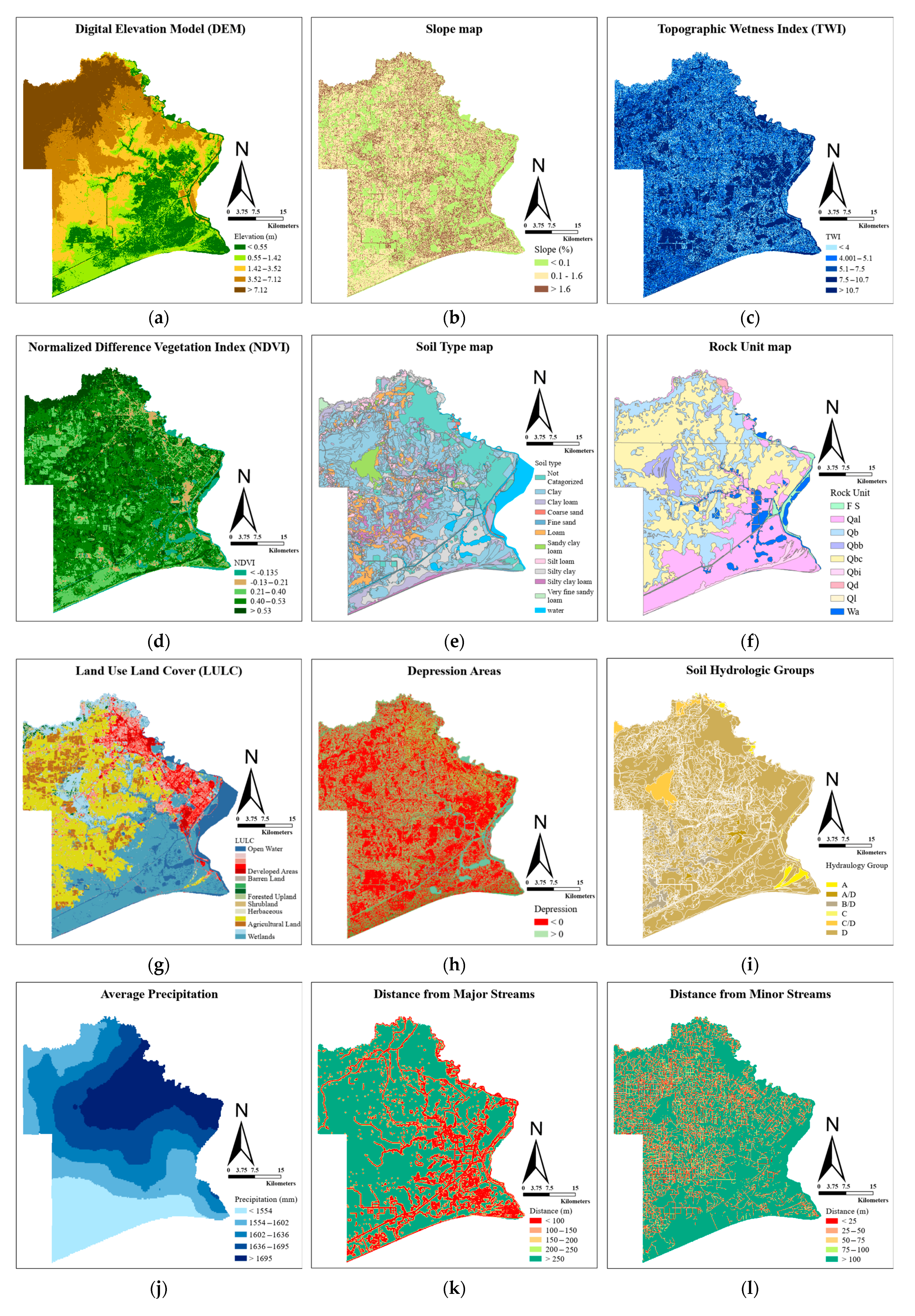
The selection of flood conditioning factors is important in effective flood susceptibility mapping, but no universally applicable scheme is available. The most relevant and most utilized factors based on the recent studies have been used in this work. A total of 13 geospatial maps were delineated to generate a flood susceptibility map, including the Elevation Model (DEM), slope, Topographic Wetness Index (TWI), Normalized Difference Vegetation Index (NDVI), Soil type, Rock unite, land-use/land-cover (LULC), Depression areas, Soil Hydrologic group, Average Precipitation, Distance from major streams, Distance from minor streams, and distance from roads (Figure 2 and Figure 3 and Table 2) [41,42,43,44,45,46,47]. A Sentinel-1 SAR map was generated with the Google Earth Engine code to retrieve data for pluvial flooded areas from 2018 to 2023 (Figure 4 and Figure 5).

2.2.1. Digital Elevation Model

DEM indicates elevation, where low-lying areas are more prone to water accumulation and flooding, while higher terrains facilitate runoff and reduce inundation risk [43]. High-resolution flood conditioning factors significantly enhance flood susceptibility mapping accuracy. Higher-resolution DEMs show more details and, consequently, they require more computational resources. Moderate-resolution DEMs (e.g., 30 m) offer a balance between accuracy and efficiency, making them widely used in flood susceptibility studies. The choice of DEM resolution also influences flood inventory mapping, which affects how well flood and non-flood areas are distinguished [49,50].
A 30 m resolution DEM is used in this study because of the time saving of the analysis, and likewise, previous research has shown that it has acceptable accuracy in generating flood susceptibility maps. in this study, 30 m DEM data were retrieved from USGS Elevation DATA.

2.2.2. Slope

Slope was derived from a Digital Elevation Model (DEM) using the Slope tool in ArcGIS Pro and calculated in percentage as a feature for both statistical and machine learning models. Areas with low slope values are more prone to flooding due to reduced runoff and poor drainage. Conversely, steeper slopes promote faster runoff, reducing water accumulation. Incorporating slope as a continuous geospatial layer allows for improved identification of flood-prone areas [51,52,53].

2.2.3. Topographic Wetness Index (TWI)

TWI reflects soil moisture potential, in which higher values present zones of water accumulation that are more likely to experience flooding [54]. TWI is calculated using the log-transformed ratio of the upslope area to the contour length (Equation (1)). In Equation (2), 0.5 is added to the denominator of the fraction to prevent division errors on flat terrain, which is used in this study, as Jefferson County is located on a flat plain area [43].
T W I = l n ( α t a n β )
T W I = l n ( α t a n β + 0.5   )
where α is the cumulative upstream discharge at one point and β is the local slope angle.

2.2.4. Normalized Difference Vegetation Index (NDVI)

Areas with high NDVI (dense vegetation) promote infiltration and reduce runoff, while low NDVI (bare or urban surfaces) increases surface flow and flood potential [55]. The Google Earth Engine script was developed to process Landsat 8 imagery to generate the NDVI map of Jefferson County, TX. Images from 1 January 2024, to 31 December 2024, were filtered; only those with less than 1% cloud cover were selected and averaged. The NDVI was calculated using the near-infrared (B5) and red (B4) bands. In the end, the NDVI image was saved with a 30-m resolution [56,57,58].

2.2.5. Soil Type

Soil type plays a key role in flood susceptibility by controlling infiltration and runoff. Sandy soils with high permeability reduce flood risk by absorbing water, while clay soils with low permeability increase surface runoff and thus higher flood risk [43,59]. The soil type retrieved from the Soil Survey Geographic Database 2.3.2 [60], updated by 30 August 2024. Based on the SSURGO database, Jefferson County is mainly covered by clay and clay loam soils, which have low permeability and poor drainage. This increases surface runoff and makes the area more vulnerable to flooding during heavy rainfall.

2.2.6. Rock Unit

Geological formations control permeability, with permeable rocks like sandstone enhancing infiltration, whereas impermeable units such as shale or granite increase surface runoff and flooding likelihood [61,62]. In Jefferson County, the majority of areas are under the Qal and Qb rockunit classifications, which are 24.60% and 70.62% of the whole area, respectively. Based on geological mapping, the Qal is classified as a very high flood hazard area that is vulnerable to riverine floods, flash floods, and debris flow. Qb refers to flood-basin deposits from the Recent age, and Qal represents undifferentiated younger and older alluvium from the Quaternary age [63,64]. Rock Unit data driven from RockUnitPoly250K, Texas (TNRIS) Geologic Data [65].

2.2.7. Land Use Land Cover

Land Use Land Cover (LULC) significantly influences flood susceptibility by influencing surface runoff and infiltration [66,67]. While urban areas with impervious surfaces and uncovered land increase runoff and flood risk, areas with high vegetation density have a lower risk of flooding due to their ability to absorb water [68]. In this study, the Land Use Land Cover (LULC) from the NLCD 2021 Land Cover (CONUS) was downloaded and classified into agricultural land, barren land, developed areas, forested upland, Herbaceous, shrubland, wetlands, and water bodies, which each affect flood dynamics differently [69]. These classes help assess flood-prone areas by determining how land cover influences inundation. Urban expansion or deforestation can change LULC over time, which can alter flood patterns and the necessity of continuous monitoring. Studies have shown a strong correlation between LULC changes and flood occurrences, emphasizing the need for sustainable land-use planning to mitigate flood risks [70,71].

2.2.8. Depression Areas

A depression is a low-lying area surrounded by higher ground, where water accumulates during rainfall and is highly suffers from nuisance flooding [72]. Pluvial flooding in urbanized areas only occurs in depressions, which hold stormwater that exceeds the capacity of urban drainage systems. These are important in urban flooding because they can store rainwater, leading to localized flooding if drainage is insufficient. Depression is simply calculated by subtracting the filled DEM from the original DEM [73,74]. In this study, to enhance the sensitivity of the susceptibility model, all filled areas are considered depression areas [75].
Depression areas = Filled DEM − Original DEM

2.2.9. Soil Hydrology Group

The soil hydrology group is downloaded from SSURGO [48] database. Based on their potential for runoff, soils have been divided into four major groups by the Natural Resources Conservation Service (NRCS). Jefferson County is characterized by all four soil hydrologic groups A, B, C, and D in which about 91.68% of the land area is in soil hydrologic group D. Soil hydrologic group D indicates that soils having very slow infiltration rates when thoroughly wetted, consisting of mostly clayey soils with high swelling capacity or potential, soils with a high permanent water table, soils with claypan or clay layer at or near the surface, and shallow soils over nearly impervious materials. These soils have a very slow rate of water transmission. The rest of the groups in Jefferson County are B/D at 3.53%, C/D at 2.89%, and group A, which is 1.1%. Group B/D shows soils that naturally have a very slow infiltration rate due to a high water table but will have a moderate rate of infiltration and runoff if drained. Soil C/D shows that soils naturally have a very slow infiltration rate due to a high water table but will have a slow rate of infiltration if drained, and group A stands for soils consisting of deep, well-drained sands or gravelly sands with high infiltration and low runoff rates.

2.2.10. Average Precipitation

Areas with high rainfall receive more water input, which increases runoff and flooding, especially during extreme events like hurricanes or intense storms [76]. Based on the rain data downloaded from the Parameter-elevation Regressions on Independent Slopes Model (PRISM) website from 2018 to 2023, the study area experienced an average annual precipitation of 1695 mm. The northeast of Jefferson County, which also consists of Beaumont city, experienced rain higher than 1695 mm, a total of 19.5% of the entire area (Figure 2 and Figure 3j) [77].
Figure 2. Yearly average flood retrieved from PRISM.
Remotesensing 17 03471 g002
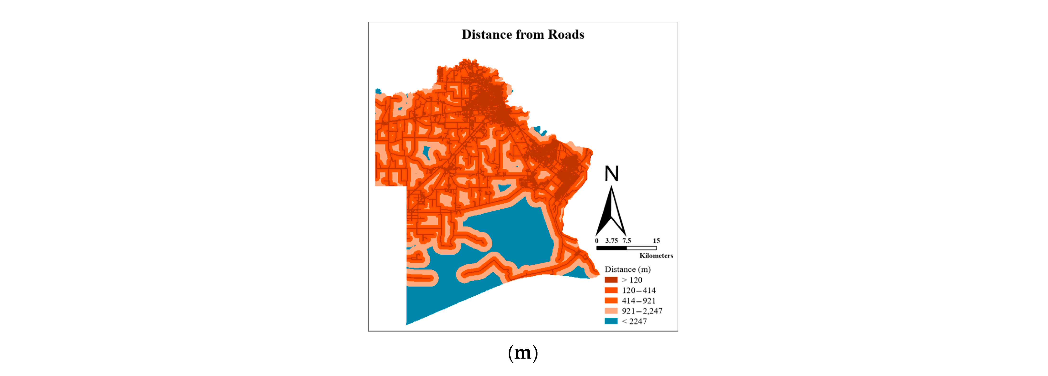
Figure 3. Geospatial layers for delineating a flood susceptibility map. (a) Dem, (b) Slope, (c) TWI, (d) NDVI, (e) Soil Type, (f) Rock Unit, (g) LULC, (h) Depression, (i) Soil Hydrology, (j) Precipitation, (k) Distance from Major Streams, (l) Distance from Minor Streams, (m) Distance from Roads.
Remotesensing 17 03471 g003aRemotesensing 17 03471 g003b

2.2.11. Distance for Streams and Waterbodies

The possibility of flooding is enhanced when an area is near rivers and canals and decreases if it is farther away. For this reason, areas near rivers and canals are given a higher vulnerability weight in comparison with those farther away [52,78]. In this article, based on the previous findings of [41,79] streams are categorized into two groups, major and minor, based on their surface width, as their behaviors are different during floods, which results from differences in their floodplains. Small ditches, canals, and rivers with surface widths less than 10 m are considered minor streams, and the rest of the water bodies are considered major. For each major and minor stream, five classification categories are considered using the Euclidean Distance tool in ArcGIS Pro 3.0.0.

2.2.12. Distance from Road

The distance from roads is an independent variable that plays a crucial role in flood risk assessment. Areas closer to roads typically have more impervious surfaces, which accelerate runoff during rainfall events, increasing the likelihood of flooding. while areas farther from roads tend to have more permeable surfaces, allowing for greater water absorption and retention, thereby reducing flood risk [46,80]. The Euclidean Distance tool in ArcGIS Pro was employed for calculation, and the result was classified into five groups based on quantile (Figure 3m).

2.2.13. Sentinel 1 SAR Image

For flood extent mapping, spectral data from optical sensors like Landsat and backscatter data from synthetic aperture radar (SAR), such as Sentinel-1, are commonly used. Optical data are preferred in cloud-free conditions due to their strong correlation with open water [81,82,83]. A JavaScript code is developed for use in Google Earth Engine (GEE) to automatically retrieve water pixels from 2018 to 2019, using Sentinel-1 SAR imagery with the following Algorithm 1:
Algorithm 1. Flood Inventory Mapping Using Sentinel-1 SAR Imagery.
Input: Sentinel-1 SAR imagery (2018–2019), PRISM rainfall data
Output: Water pixels map
(1)
Obtain rainy and dry dates from PRISM to distinguish wet and dry days.
(2)
For each rainy day:
  Select the nearest subsequent Sentinel-1 SAR image.
(3)
For each dry date:
Select the nearest Sentinel-1 image to the corresponding wet image, ensuring ≥15 consecutive dry days before selection.
(4)
Apply a water mask with VV polarization threshold (<−13.05 dB) and perform speckle noise filtering.
(5)
Define water layers:
  • waterWet: water pixels during wet day
  • waterDry: water pixels during dry day
  • waterDry.eq(0): pixels not water in dry day
  • waterWet. and (waterDry.eq(0)): pixels wet in wet day AND not wet in dry day
(6)
Integrate all generated images for each year.
(7)
Retain only water pixels that appear repeatedly for ≥3 years to reduce noise and increase reliability.
The −13.05 dB VV threshold for Sentinel-1 was adopted from Islam and Meng [84], who calibrated it over Houston City, Texas. This threshold is considered for Jefferson County because both areas lie within the Gulf Coastal Plain of Southeast Texas, sharing low-lying topography, humid subtropical climate, and frequent pluvial (ponding) flooding conditions. In terms of proximity, Houston City (≈29.76°N, 95.37°W) is ~80 miles from the Jefferson County study area (≈29.82°N, 94.15°W).
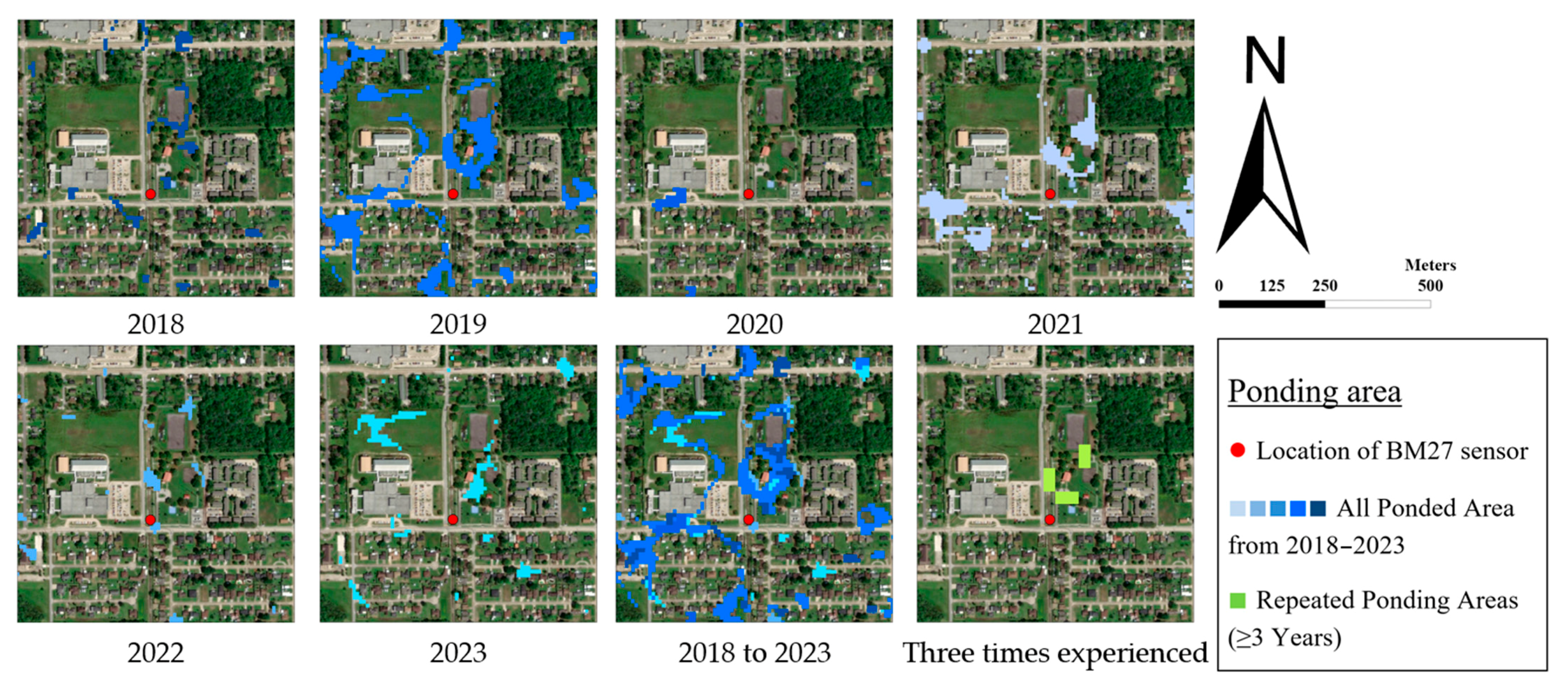
Figure 4. VV Sentinel-1 image 2018–2023. (BM27 Location: 30.0423000, −94.1092000).
Remotesensing 17 03471 g004
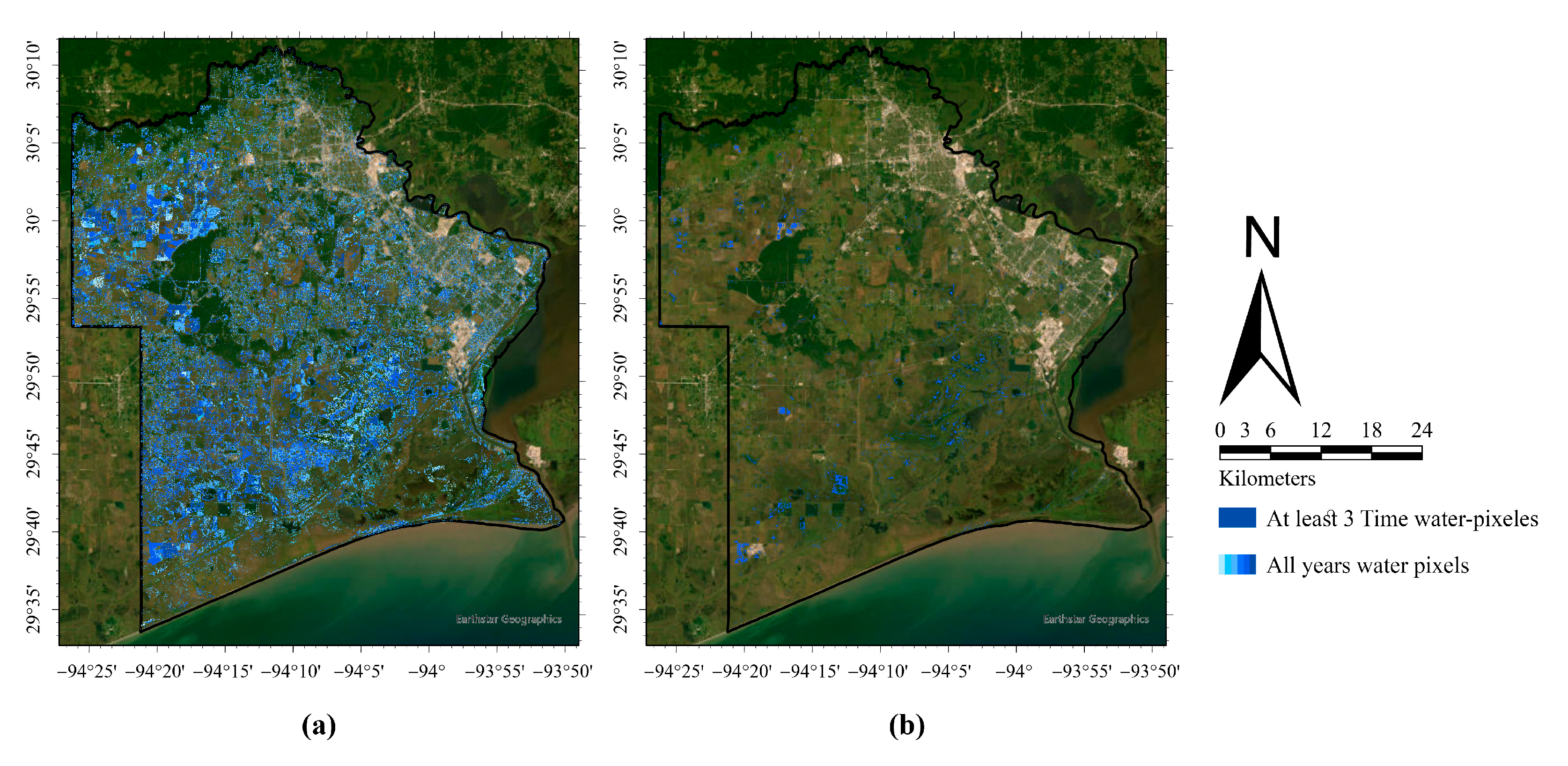
A susceptible location is defined as a spatial cell that experiences multiple water pixel occurrences over the study period. Classifying cells based on a single water pixel observation can lead to overestimation, capturing many areas that may have been affected by isolated or incidental events. On the other hand, requiring flood occurrence in all six years is too stringent and may exclude areas that are moderately but consistently at risk. Therefore, those areas that experience at least three times water pixel occurrences during the study period are considered for the target of the model (Figure 4 and Figure 5Table 3).
Figure 5. VV Sentinel-1 image 2018–2023—(a) All detected water pixels, (b) Water pixels that repeated at least 3 times.
Remotesensing 17 03471 g005

2.3. Methodology

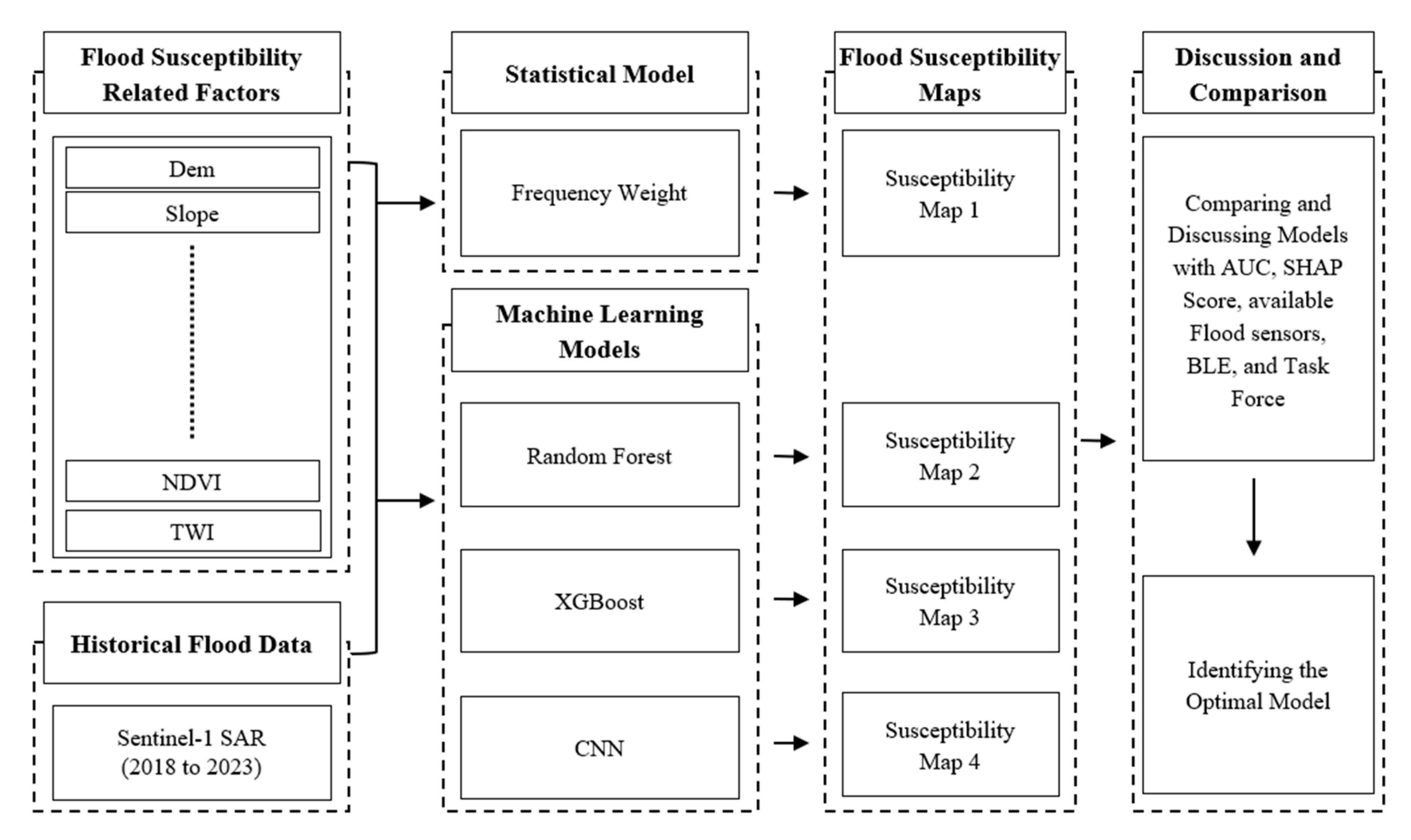
The methodology of this study is divided into four main stages. Steps 1 and 2 fall under data preparation and are explained in detail in the flood susceptibility factors and data preparation section, while Steps 3 and 4 focus on model development and evaluation for flood susceptibility mapping (Figure 6).
Step 1. Data Preparation and Map Creation:
Thirteen geospatial conditioning factors were collected and processed to support flood susceptibility analysis. These included topographic (DEM, slope, TWI), environmental (NDVI, LULC, soil type, rock unit), hydrological (precipitation, soil hydrologic group, depression areas), and proximity factors (distance to roads, major streams, and minor streams). All datasets were standardized and converted into geospatial maps in a GIS environment. ArcGIS Pro was utilized for spatial delineation, ensuring accurate integration and processing of these layers. The feature space for modeling was ultimately constructed using these 13 geospatial layers (Figure 3).
Step 2. Flood Inventory Using Sentinel-1 SAR Imagery:
A flood inventory map was produced by processing Sentinel-1 SAR images from 2018 to 2023 in Google Earth Engine. Water pixels were extracted, and repeated occurrences (≥3 times) were classified as flood-prone to reduce incidental errors. The target variable was established as a binary classification label, where flooded areas were assigned a value of 1 and non-flooded areas a value of 0.
Step 3. Flood Susceptibility Mapping:
Flood susceptibility maps were generated through two complementary approaches:
  • Statistical Model (Frequency Ratio, FR): The FR method was applied to calculate the relative likelihood of flooding for each class of conditioning factors, providing a baseline statistical assessment of susceptibility.
  • Machine Learning Models: three machine learning models, Random Forest, XGBoost, and Convolutional Neural Networks (CNN), were employed to generate flood susceptibility maps. Random Forest and XGBoost were selected as tree-based algorithms, which are widely recognized as effective models for tabular datasets. Random Forest used as a robust ensemble method with relatively simple structure and interpretability, whereas XGBoost, as an advanced boosting algorithm, was included to capture complex nonlinear relationships and interactions feature space. The CNN model was also introduced as a deep learning architecture capable of learning local feature dependencies and nonlinear patterns across the geospatial predictors.
Step 4. Model Evaluation and Comparison:
The resulting susceptibility maps from both the statistical and machine learning approaches were compared against available high-risk locations, the Base Level Engineering (BLE) map, and input from the Local Community Task Force to assess their accuracy and practical relevance. Model performance was quantitatively evaluated using the Area Under the ROC Curve (AUC), while SHAP values were computed for the machine learning models to explain the contribution of each conditioning factor. This multi-layered validation ensured both predictive accuracy and interpretability of the models for flood risk management.

2.3.1. Model Development

Statistical Model
Frequency ratio calculations: The Frequency Ratio (FR) applies bivariate statistical analysis to link flood frequency with independent variables, reflecting the principle that past flood events can occur again under similar conditions. FR scores are quantitative, where values above 1 indicate a higher likelihood of flooding, while scores below 1 suggest lower susceptibility [85,86,87,88,89,90,91]. The frequency ratio (FR) is determined by analyzing the percentage of ponding occurrences (water-pixels) within each class of a given geospatial layer. Each layer is categorized into distinct classes by quantile or its own classification scheme, and for major and minor streams and distance from roads, classifications from previous studies were adopted, as already explained in the data preparation section. All maps are illustrated in Figure 3. First, the percentage of each class relative to the entire layer is computed. Next, the percentage of ponding events occurring within each class is calculated. The FR is then obtained by dividing the event percentage by the class area percentage and multiplying the result by 100, thereby assigning a weight to each class area.
Machine Learning
i. 
Model Preprocessing
Data Normalization: In this study, normalization was applied as a preprocessing step for the Convolutional Neural Network (CNN) model. Neural networks are sensitive to the scale of input variables, and normalization improves training stability and convergence by reducing the risk of exploding or vanishing gradients. For this purpose, the features used in the CNN were standardized using the Standard Scaler transformation. In contrast, Random Forest and XGBoost models were trained directly on raw feature values, as tree-based algorithms rely on threshold-based splitting rules and are inherently insensitive to feature scaling.
Training–Testing Split and Cross-Validation: The binary flood occurrence (water pixels) dataset used for machine learning was inherently imbalanced, with only 1.7% water pixels (positive class) compared to 98.3% non-water pixels (negative class). To ensure reliable evaluation of model performance, the dataset was divided into training and testing subsets using stratified sampling. This approach maintained the original proportion of flooded and non-flooded pixels in both sets, which was particularly important given the class imbalance. In addition, stratified k-fold cross-validation was applied during model training, ensuring that class distributions were preserved across folds and reducing the risk of biased evaluation.
Hyperparameter Tuning: The optimization procedure was carried out through three main steps. First, the dataset was divided into multiple stratified folds to preserve class proportions across both training and validation subsets. Next, an optimization function was defined to calculate the AUC score of each model configuration on the validation data. Finally, the optimum parameters were estimated by identifying the configuration that achieved the maximum AUC score among the randomly sampled hyperparameter sets.
ii. 
Models
Random Forest: Random Forest (RF) is an ensemble learning algorithm that constructs multiple decision trees using a bagging approach, making it effective for both classification and regression tasks. It leverages the advantages of decision trees, such as adaptability to missing values and robustness, while addressing their limitations, including sensitivity to noise and overfitting [92]. RF operates by training individual decision trees on randomly selected subsets of data and features, then aggregating their outputs through majority voting for classification or averaging for regression. In the RF algorithm, a random vector ik (representing a conditioning factor) is independently generated for each tree and distributed across all trees. This results in a collection of tree-structured classifiers h(x,ik) for input vector x. The trees are grown using both the training dataset and the random vector x, ensuring diversity among the classifiers. RF effectively handles feature correlations without requiring special adjustments and adapts well to various data distributions [93,94].
One of RF’s notable strengths is its interpretability; it can assess the importance of each feature by analyzing its contribution across decision trees. Additionally, RF’s hyperparameter tuning process is relatively simple, making it practical for real-world applications.
XGBoost: XGBoost (eXtreme Gradient Boosting) is a state-of-the-art boosting algorithm that improves upon traditional gradient boosting methods by optimizing computational efficiency, regularization techniques, and handling of missing values. Introduced by Chen and Guestrin [95], XGBoost has been widely applied in data science competitions and real-world applications due to its robustness and scalability. In this study, XGBoost is used to find the relationship between hydrological and geospatial features and flood susceptibility. XGBoost follows an additive model where a weak learner (a decision tree) is added at each iteration to minimize the loss function. The prediction at the K times iteration is given by
y ˆ i ( K ) = y ˆ i ( K 1 ) + f K x i
where
  • y ˆ i ( K ) is the predicted output after K boosting rounds.
  • f K x i is the newly added decision tree.
The objective function consists of two main components: the training loss and the regularization term:
L = i = 1 n l y i , y ˆ i + k = 1 K Ω f k
where
  • l y i , y ˆ i represents the loss function (e.g., log-loss for binary classification).
  • Ω f k is the regularization term, which helps prevent overfitting and is defined as
Ω f k = γ T + 1 2 λ ω 2
where
  • T is the number of leaves in the tree.
  • γ and λ are regularization hyperparameters.
  • ω represents leaf weights.
CNN: A Convolutional Neural Network (CNN) was employed as one of the deep learning architectures, as it can capture spatial patterns and feature interactions from multi-layer input data. For flood susceptibility mapping, environmental and topographic variables often interact in complex ways that are not easily represented by conventional methods, and CNNs provide a framework to model these spatial dependencies.
The CNN developed in this study was designed to take 13 geospatial predictor layers as input and process them through convolutional, pooling, and dense layers. The convolutional layers were used to detect patterns and interactions across the input features, while pooling layers reduced the size of the data and kept the most important information. The dense layers then combined these learned features and produced the final classification. The model was trained using the Adam optimizer with binary cross-entropy loss, and a sigmoid activation function was applied in the output layer for binary classification. The overall architecture of the CNN is presented in Figure 7.

2.3.2. Model Evaluation

  • ROC Curve (AUC) metric
The Area Under the Curve (AUC) is derived from the Receiver Operating Characteristic (ROC) curve, which illustrates a model’s classification performance across different probability thresholds. The ROC curve plots the True Positive Rate (TPR) against the False Positive Rate (FPR), where TPR represents the proportion of actual positives correctly identified, and FPR represents the proportion of actual negatives incorrectly classified as positive. By adjusting the probability threshold used to convert predicted probabilities into binary outcomes, different true positive and false positive rates are produced, forming the ROC curve. The AUC score summarizes this curve into a single value between 0 and 1, where a value closer to 1 indicates excellent discriminative ability. In the context of flood susceptibility mapping, a higher AUC means the model is more capable of distinguishing between flood-prone and non-flood-prone areas over all threshold levels. The formulas for TPR and FPR are given by
T P R = T P T P + F N
F P R = F P F P + T N
where
TP (True Positive) = number of ponding-prone areas correctly predicted as flood-prone
FN (False Negative) = number of ponding-prone areas incorrectly predicted as non-flood-prone
FP (False Positive) = number of non-ponding-prone areas incorrectly predicted as flood-prone
TN (True Negative) = number of non-ponding-prone areas correctly predicted as non-flood-prone
ii.
SHAP Value Interpretability
SHAP values help to explain the spatial patterns seen in flood susceptibility maps by showing each feature’s impact on the output of the model [96,97]. They ensure model transparency and offer stakeholders evidence-based explanations for why certain regions are flagged as high or low-risk. This interpretability is vital for guiding infrastructure planning, flood mitigation efforts, and emergency response strategies [96,98,99]. SHAP values help to explain the spatial patterns seen in flood susceptibility maps by showing each feature’s impact on the output of the model [96,97]. They ensure model transparency and offer stakeholders evidence-based explanations for why certain regions are flagged as high or low-risk. This interpretability is vital for guiding infrastructure planning, flood mitigation efforts, and emergency response strategies [96,98,99].
iii.
Validation by High-Risk Locations
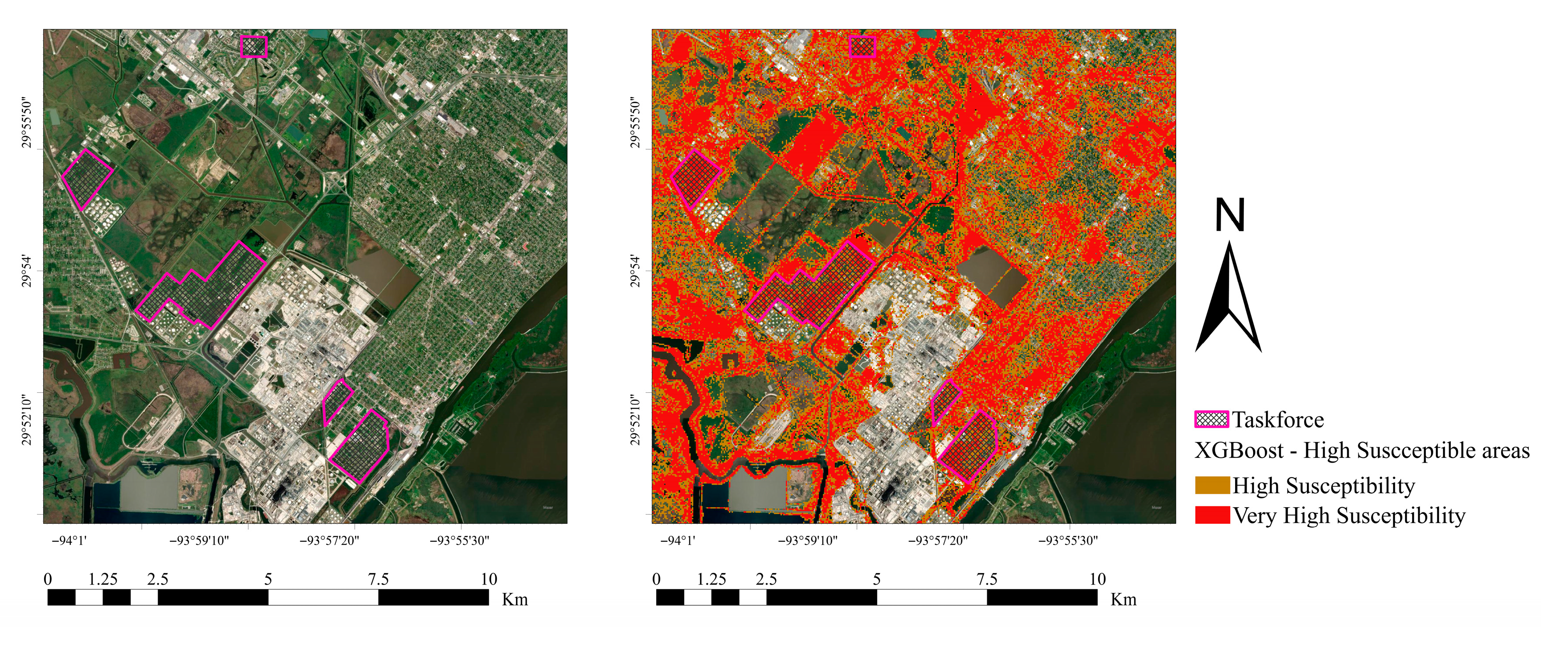
The high-flood-risk locations in Jefferson County are monitored by flood sensors, identified by local agency experts based on past flooding events and historic high-water marks [100]. In addition, the Local Community Task Force, which includes senior engineers and experts from the Jefferson County Drainage Districts, Texas Department of Transportation (TxDOT), U.S. Department of Energy (DOE), and other local agency experts, identified high flood-risk areas, many of which have historically been prone to flooding. Consequently, an effective model should be able to classify the majority of high-risk locations into high or very high flood-susceptibility zones.
iv.
Comparison with BLE Maps
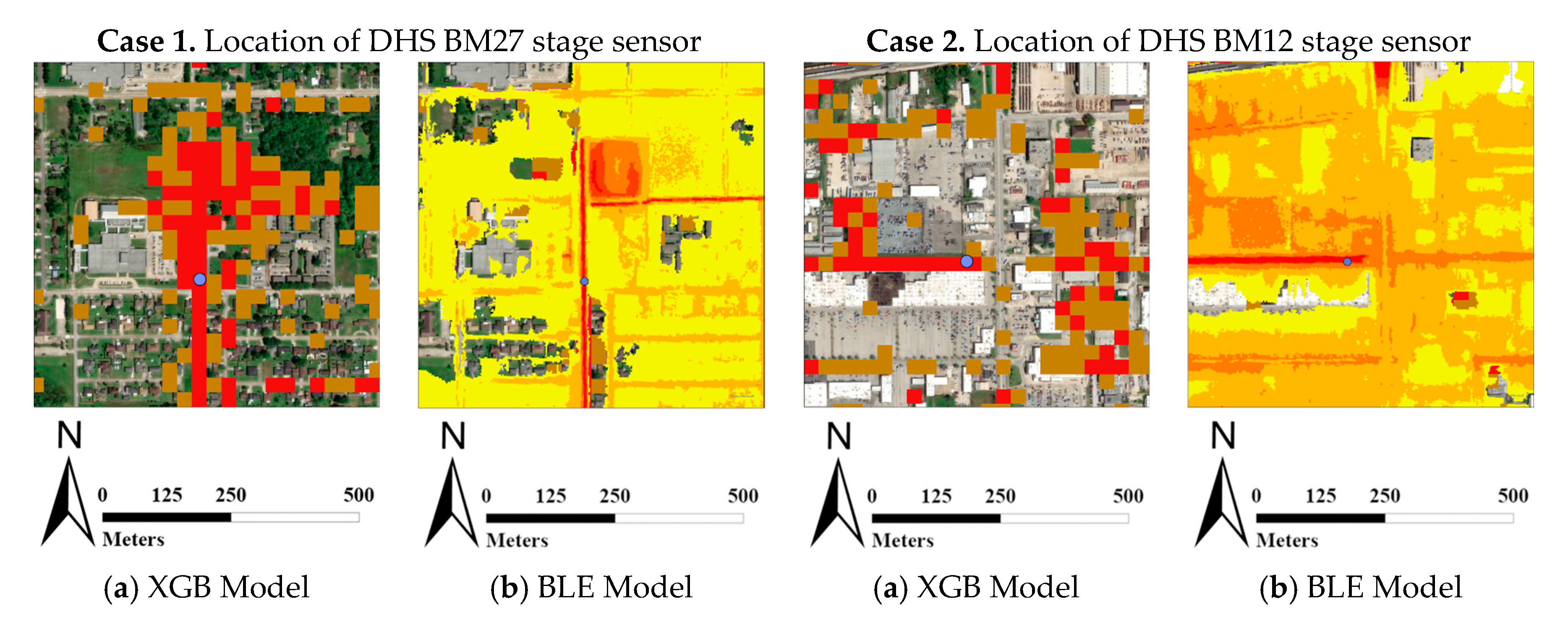
Base Level Engineering (BLE) is a flood-mapping methodology designed to provide hazard information in ungauged or understudied areas. The BLE_DEP0_2PCT dataset quantifies estimated flood depths within the 1% annual chance floodplain by subtracting ground elevation from modeled water surface elevations, thereby generating raster-based flood depth values [101].

3. Results and Discussion

This section presents a comprehensive evaluation of the flood susceptibility modeling results. First, a correlation analysis is conducted to assess and address potential multicollinearity, followed by an evaluation of AUC scores to compare the predictive performance of different models. Then, SHAP values are analyzed to identify the most influential features. Following this, the generated flood susceptibility maps illustrate how each model delineates areas of potential flood risk. Finally, the models are validated against high-risk locations monitored by sensors, community task force flood-prone areas, and reference maps from BLE.

3.1. Correlation Analysis

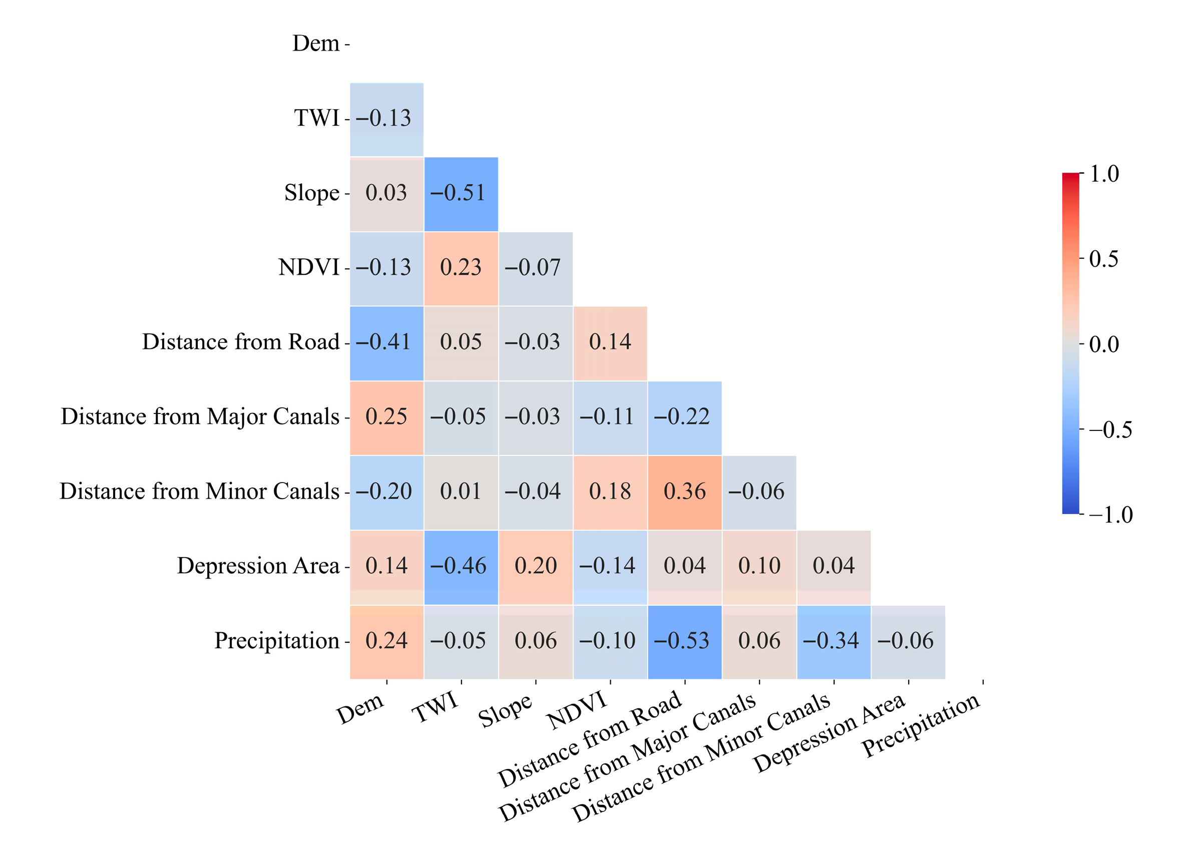
As illustrated (Figure 8), the maximum and minimum correlation values among the continuous variables are 0.36 and −0.53, respectively. These results indicate that the continuous features are linearly independent and can therefore be used in the machine learning algorithms without concerns regarding multicollinearity. This independence helps ensure that the predictive models are not affected by high variance caused by highly correlated features and confirms that selected variables are proper for robust model development.

3.2. Statistical Model Results

The frequency ratio (FR) results show that flood susceptibility is strongly influenced by topography, distance to rivers, land use, and soil characteristics. Low elevations, low-gradient slopes, and areas within 100 m of rivers have high FR values, confirming they are the most flood-prone. Similarly, zones with high topographic wetness index (TWI), depressions, poorly draining soils (Group D), and agricultural or wetland land uses exhibit higher susceptibility, as they limit infiltration. In contrast, higher elevations, steep slopes, forested land, and areas far from rivers have FR < 1, indicating low flood risk (Table 4).
The model highlights that flood-prone areas are concentrated in low-lying, flat, and poorly drained regions, near rivers and wetlands, while well-vegetated and elevated zones remain relatively safe.

3.3. Machine Learning Model

3.3.1. Hyperparameter Tuning

Hyperparameter optimization was conducted for both the Random Forest and XGBoost models to improve predictive performance. For the Random Forest, the parameter space included n_estimators, max_depth, min_samples_split, and min_samples_leaf. For the XGBoost model, the parameter space consisted of lambda, alpha, colsample_bytree, subsample, learning_rate, n_estimators, max_depth, and min_child_weight. The optimum hyperparameters obtained for both models are summarized in the Table 5.

3.3.2. AUC Score

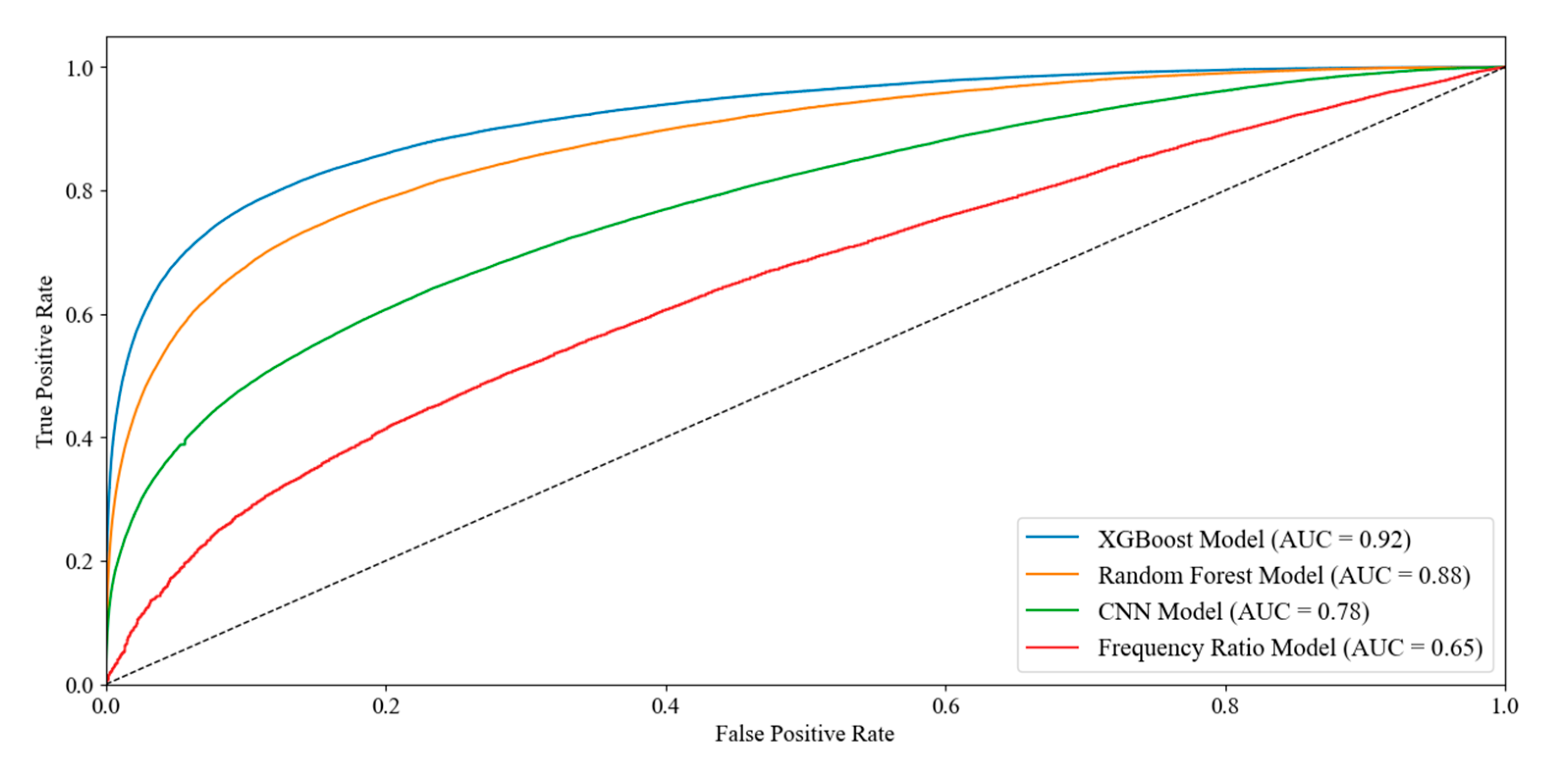
Among the models tested, XGBoost achieved the highest AUC of 0.92, confirming its superior ability to distinguish flood-prone from non-flood-prone areas. This aligns with its SHAP analysis, which revealed strong, targeted feature impacts for critical variables such as elevation, slope, and TWI. Additionally, XGBoost correctly classified the highest risk locations (100) in high or very high susceptibility zones, further validating its practical effectiveness. Random Forest, with an AUC of 0.88, also performed well and matched high-risk locations reasonably, though its SHAP values were more conservative. The CNN model had a lower AUC of 0.78, consistent with earlier findings that it underestimates risk, as it misclassified many flood-prone areas into low-susceptibility zones. Lastly, the Frequency Ratio model, with the lowest AUC of 0.65, lacked the complexity to model flood patterns accurately. These results clearly show that XGBoost offers the best balance of accuracy, interpretability, and real-world alignment, making it the most effective model for flood susceptibility prediction in Jefferson County (Figure 9).

3.3.3. SHAP Score

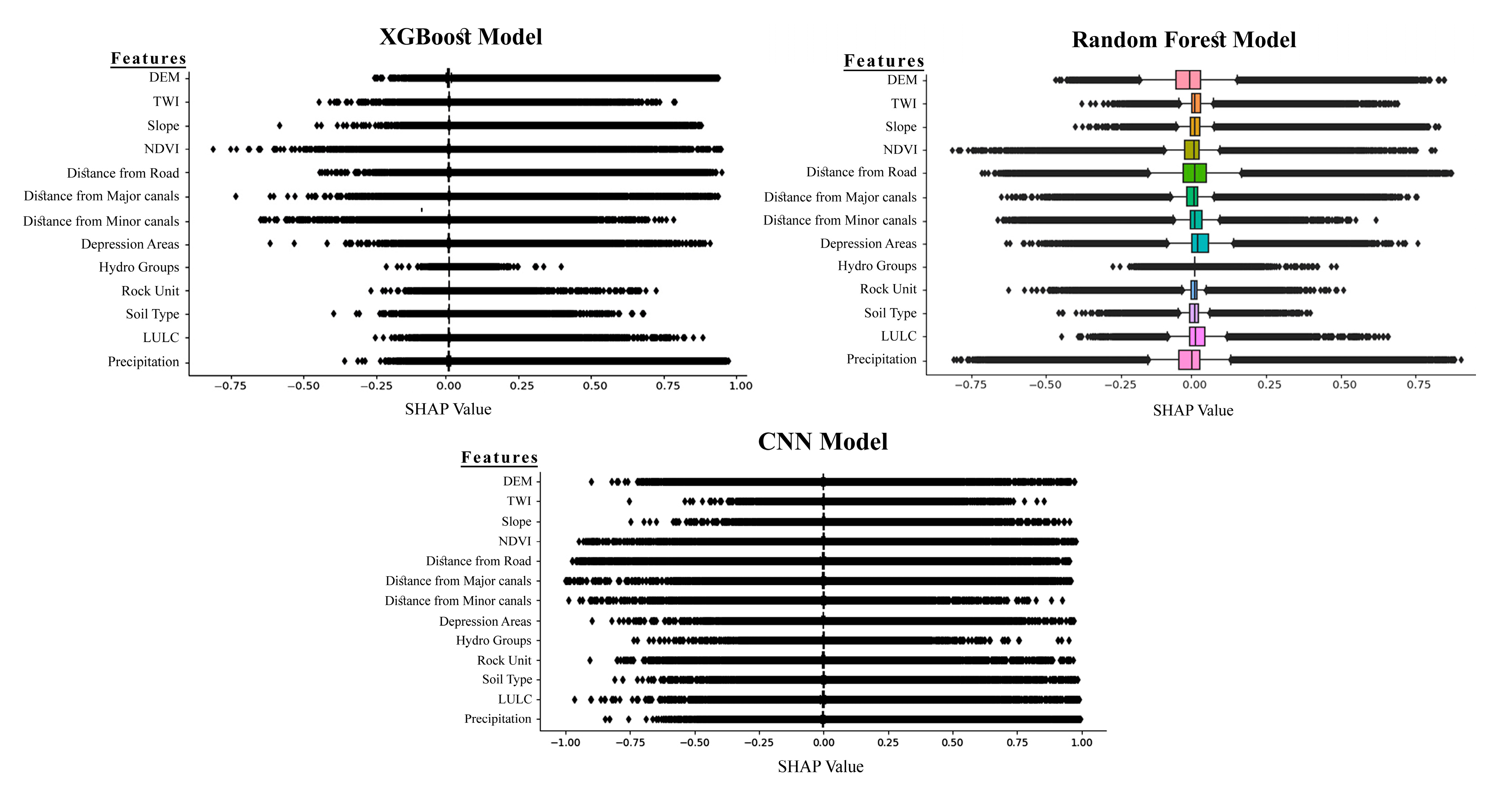
The SHAP value results from the CNN, Random Forest, and XGBoost models collectively offer strong insight into the role of various environmental and geospatial features in predicting flood susceptibility (Figure 10). Across all three models, elevation (DEM), Topographic Wetness Index (TWI), slope, NDVI, and distance to rivers or canals consistently emerge as the most influential features, confirming their critical roles in flood risk. Low elevation and flat terrain strongly increase flood susceptibility, as indicated by positive SHAP values, while higher elevations and steeper slopes have negative SHAP impacts, reducing predicted flood risk. TWI and NDVI further refine this by identifying areas prone to water accumulation or sparse vegetation, both conditions that heighten flood vulnerability. CNN and XGBoost tend to assign broader SHAP value ranges, meaning they respond more sharply to high-risk conditions compared to the Random Forest model, which produces more conservative, narrowly distributed SHAP values [102]. XGBoost emphasizes extreme flood-prone areas more than safe zones, evident in its asymmetric SHAP distribution, whereas CNN shows a more balanced response across the risk spectrum. In contrast, the Random Forest model shows many features with zero SHAP values, particularly for less impactful variables like soil type, rock unit, land cover (NLCD), and long-term precipitation, indicating they often do not affect predictions in that model. However, the models still agree that these features are less critical overall.

3.4. Flood Susceptibility Maps

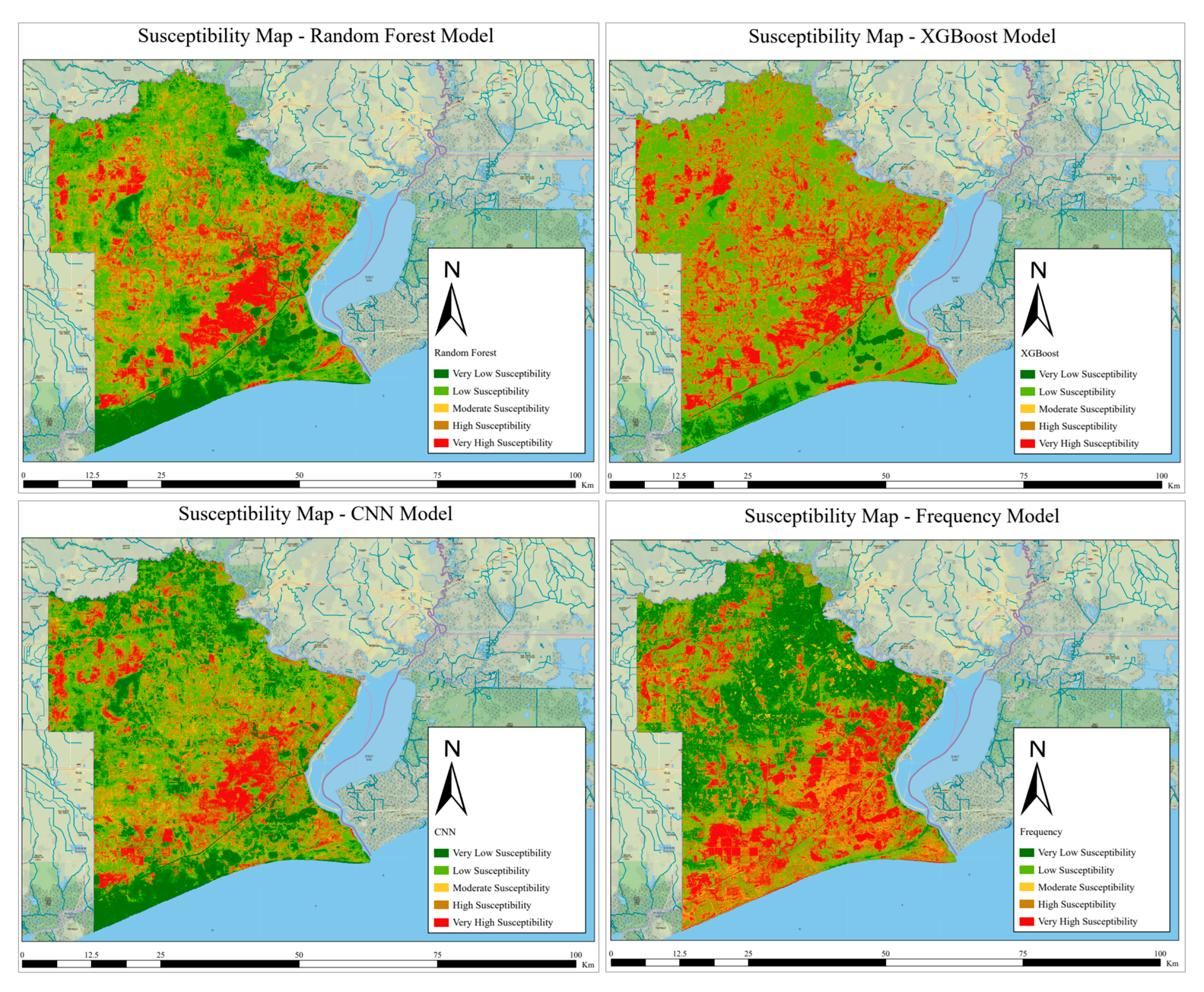
Four different flood susceptibility maps were delineated using machine learning and flood frequency weights data in ArcGIS Pro. The flood frequency weight model as a statistical model, results reveal significant variations in flood susceptibility based on topographic, hydrologic, and environmental factors. Dem (<0.55), Lower slope areas (<0.1°) and regions closer to major streams (<100 m) exhibit notably higher flood susceptibility. Additionally, higher Topographic Wetness Index (TWI > 10.7) and specific land-use categories such as barren lands and grasslands have markedly elevated susceptibility. Soil type plays a critical role, with fine sand and sandy clay loam demonstrating notably high weights. Hydrologic groups A and B/D also indicate increased flood occurrence. To help visualize the results, the continuous flood risk values were grouped into five classes: very low, low, moderate, high, and very high susceptibility, using a quantile classification method. This method helps show changes across the area more clearly and avoids using fixed intervals. The maps showed similar patterns in areas marked as very low and low risk, especially in higher or sloped land. But there were noticeable differences in areas with moderate to very high risk, mostly in flat, low-lying regions with water pixel concentration in their target. These high-risk areas were mainly found in the central and southern parts of Jefferson County (Figure 11).

3.5. High Flood-Risk Locations Monitored by Flood Sensors

Figure 12 illustrates the effectiveness of each model, including Frequency Weight, Random Forest, XGBoost, and CNN, in capturing flood-prone areas based on the high-flood-risk locations. Looking at the results, the XGBoost model shows the best alignment with high-risk locations: 39 high-risk locations fall in the “High Susceptibility” category and 61 in the “Very High Susceptibility” category, totaling 100 high-risk locations (out of 121). This is the highest concentration of sensors in flood-prone zones among all models, indicating that XGBoost can map the areas with the highest perceived flood risk. The Random Forest model is slightly behind, with 66 high-risk locations classified as high or very high susceptibility. CNN, on the other hand, only places 50 high-risk locations in these top two risk categories, suggesting it may underpredict flood hazards in historically vulnerable areas.
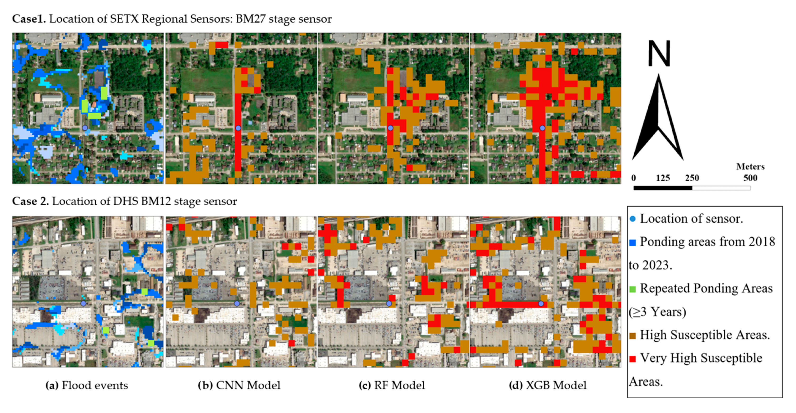
Two locations were selected for the study, both recognized as high-risk areas monitored by flood sensors BM27 and BM12. Case 1, associated with flood sensor BM27, is located in a residential area that includes a ditch designed to direct excess floodwater along the street. Case 2, linked to flood sensor BM12, represents another high-risk location that is fully developed with impervious concrete pavement and streets, also with a ditch to direct excess floodwater. In Figure 13, in the first row, all three models, CNN, RF, and XGBoost, successfully identify a high-risk location monitored by sensor BM27 within a very high flood susceptibility zone (red area), demonstrating basic model competence. However, the XGBoost model outperforms the others by identifying neighboring locations as high-risk areas that closely align with water pixel patterns shown in blue. While CNN and RF models produce dispersed predictions around the high-risk locations, XGBoost captures a broader, more realistic spatial extent of vulnerability. In the second row, for sensor BM12, the performance of XGBoost becomes even clearer, as it maps a concentrated and well-defined high-risk zone around the sensor, in strong agreement with water pixel concentration. CNN and RF fail to provide the same spatial consistency, offering scattered predictions that miss portions of the flooded region. Overall, XGBoost demonstrates better accuracy and reliability in both detecting known flood-prone zones and representing the surrounding areas at risk.

3.6. Comparison with the BLE Map

Compared with the Base Level Engineering (BLE), BLE_DEP0_2PCT also shows a good agreement with the XGBoost Flood susceptibility map. Although some areas were not detected, it’s because the XGBoost model is based on pluvial information, while BLE_DEP0_2PCT is a raster dataset class that contains the estimated flood depth throughout the 1% annual chance floodplain determined during the Base Level Engineering assessment. This dataset is compiled by performing a calculation to remove the ground elevation from the water surface elevation dataset, thereby calculating the depth of flooding expected within the 1% annual chance floodplain extents (Figure 14).

3.7. High-Risk Areas Identified by the Local Community Taskforce

All of these areas were also classified as highly susceptible by the XGBoost model (Figure 15).

4. Conclusions

The study developed a flood inventory using multi-year Sentinel-1 SAR data (2018–2023). Based on this inventory, a Frequency Ratio analysis and three machine learning models, Random Forest, CNN, and XGBoost, were then applied to generate flood susceptibility maps, identifying high-frequency ponding hot spots across Jefferson County. The maps were validated against known high-risk areas, the BLE risk map, and the community task force.
  • The alignment of the XGBoost model with the BLE risk map and the community task force assessments indicates strong qualitative agreement and model reliability.
  • The XGBoost model achieved the best performance (AUC = 0.92), correctly classifying 100 of 121 sensor-identified high-risk locations, outperforming all other methods. Random Forest showed good accuracy (AUC = 0.88) but underestimated severity, while CNN (AUC = 0.78) misclassified many high-risk areas. The Frequency Ratio model had the weakest predictive power (AUC = 0.65), confirming XGBoost as the most reliable approach for flood susceptibility mapping in Jefferson County.
  • SHAP value analysis further validated the XGBoost model interpretability, revealing that elevation, slope, TWI, and NDVI were consistently the most influential features. This helps researchers, engineers, and policymakers by highlighting the key environmental factors that drive flood susceptibility.
  • Policymakers can use flood susceptibility maps to identify high-risk hotspots and develop optimized early warning systems. By integrating these maps with real-time rainfall and sensor data, flood-prone areas can be predicted more accurately. This supports timely alerts, efficient resource allocation, and improved evacuation planning, ultimately enhancing community preparedness and reducing losses.
This study utilized six years of Sentinel-1 SAR-derived water pixel data to model flood susceptibility; however, the lack of comprehensive real flood event records may have limited the results’ precision. Using finer-resolution DEM and radar imagery could improve model accuracy but would significantly increase computation time. Further optimization of VV and VH polarization thresholds for the area of study and the inclusion of a hydrological inundation model can enhance classification around major and minor river networks. Future research should refine geospatial factors to improve susceptibility accuracy and test the methodology in mountainous regions, with the related variables, which could strengthen the reliability and generalizability of the approach.

Author Contributions

Conceptualization, M.F. and N.B.; methodology, M.F., N.B. and H.A.; software, M.F., H.A. and H.H.A.; validation, M.F., H.A. and H.H.A.; formal analysis, H.A. and M.F.; investigation, M.F. and K.W.; resources, N.B.; data curation, M.F., H.A. and K.W.; writing—original draft preparation, M.F. and H.A.; writing—review and editing, M.F., N.B., H.A. and H.H.A.; visualization, M.F.; supervision, N.B.; project administration, N.B.; funding acquisition, N.B. All authors have read and agreed to the published version of the manuscript.

Funding

This research was funded by U.S. Department of Energy, Office of Science, Biological and Environmental Research Program under Award Number DE-SC0023216, and the Center for Resiliency (CfR) at Lamar University.

Data Availability Statement

The raw data supporting the conclusions of this article will be made available by the authors on request.

Conflicts of Interest

The authors declare no conflicts of interest.

References

  1. Sharif, H.O.; Yates, D.; Roberts, R.; Mueller, C. The use of an automated nowcasting system to forecast flash floods in an urban watershed. J. Hydrometeorol. 2006, 7, 190–202. [Google Scholar] [CrossRef]
  2. Ellis, K.N.; First, J.M.; Strader, S.M.; Grondin, N.S.; Burow, D.; Medley, Z. The climatology, vulnerability, and public perceptions associated with overlapping tornado and flash flood warnings in a portion of the southeast United States. Weather Clim. Soc. 2023, 15, 943–961. [Google Scholar] [CrossRef]
  3. First, J.M.; Ellis, K.; Strader, S. Double trouble: Examining public protective decision-making during concurrent tornado and flash flood threats in the US Southeast. Int. J. Disaster Risk Reduct. 2022, 81, 103297. [Google Scholar] [CrossRef]
  4. Iglesias, V.; Braswell, A.E.; Rossi, M.W.; Joseph, M.B.; McShane, C.; Cattau, M.; Koontz, M.J.; McGlinchy, J.; Nagy, R.C.; Balch, J. Risky development: Increasing exposure to natural hazards in the United States. Earth’s Future 2021, 9, e2020EF001795. [Google Scholar] [CrossRef] [PubMed]
  5. Summers, J.; Lamper, A.; McMillion, C.; Harwell, L. Observed changes in the frequency, intensity, and spatial patterns of nine natural hazards in the United States from 2000 to 2019. Sustainability 2022, 14, 4158. [Google Scholar] [CrossRef]
  6. Li, H. A Multi-Attribute Method for Ranking the Risks from Multiple Hazards in a Small Community; Massachusetts Institute of Technology: Cambridge, MA, USA, 2007. [Google Scholar]
  7. (NWS), N.W.S. Flood Fatalities. Hydrologic Information Center. 2014. Available online: http://nws.noaa.gov/oh/hic/flood_stats/recent_individual_deaths.shtml (accessed on 10 March 2014).
  8. Service, N.W. Summary of Natural Hazard Statistics for 2013 in the United States; National Oceanic and Atmospheric Administration, US Department of Commerce: Silver Spring, MD, USA, 2014. [Google Scholar]
  9. FEMA. Texas Historical Flood Information. 2025. Available online: https://www.cityofcorinth.com/engineering/page/fema-texas-historical-flood-information (accessed on 23 March 2025).
  10. NOAA. Tropical Cyclone Point Maxima. 2025. Available online: https://www.wpc.ncep.noaa.gov/tropical/rain/tcmaxima.html (accessed on 23 March 2025).
  11. Han, Z.; Sharif, H.O. Analysis of flood fatalities in the United States, 1959–2019. Water 2021, 13, 1871. [Google Scholar] [CrossRef]
  12. Vipulanandan, C.; Parameswaran, S. Hurricane Harvey survey assessment and lessons learned. In Proceedings of the Texas Hurricane Center for Innovative Technology Conference and Exhibition, Houston, TX, USA, 3 August 2018. [Google Scholar]
  13. Center, N. National Hurricane Center; Honolulu Forecast Office: Honolulu, HI, USA, 2005. [Google Scholar]
  14. Blake, E.; Zelinsky, D. National Hurricane Center Tropical Cyclone Report Hurricane Harvey (AL092017) 17 August–1 September 2017; NOAA National Hurricane Center: Miami, FL, USA, 2018. [Google Scholar]
  15. Asli, H.H.; Brake, N.; Kruger, J.; Haselbach, L.; Adesina, M. Field surveying data of low-cost networked flood sensors in southeast Texas. Data Brief 2023, 50, 109504. [Google Scholar] [CrossRef] [PubMed]
  16. Haselbach, L.; Thies, C.; Evans, H.; Apple, C.; Tindall, N. Findings from Two Flood Disaster Response Exercises for Southeast Texas. In Leveraging Sustainable Infrastructure for Resilient Communities; ASCE: Reston, VA, USA, 2022; pp. 22–33. [Google Scholar]
  17. Vilasan, R.T.; Kapse, V.S. Evaluation of the prediction capability of AHP and F-AHP methods in flood susceptibility mapping of Ernakulam district (India). Nat. Hazards 2022, 112, 1767–1793. [Google Scholar] [CrossRef]
  18. Latif, R.M.A.; He, J. Flood Susceptibility Mapping in Punjab, Pakistan: A Hybrid Approach Integrating Remote Sensing and Analytical Hierarchy Process. Atmosphere 2024, 16, 22. [Google Scholar] [CrossRef]
  19. Fatah, K.K.; Mustafa, Y.T. Flood susceptibility mapping using an analytic hierarchy process model based on remote sensing and GIS approaches in Akre District, Kurdistan Region, Iraq. Iraqi Geol. J. 2022, 55, 121–149. [Google Scholar] [CrossRef]
  20. Yilmaz, O.S. Flood hazard susceptibility areas mapping using Analytical Hierarchical Process (AHP), Frequency Ratio (FR) and AHP-FR ensemble based on Geographic Information Systems (GIS): A case study for Kastamonu, Türkiye. Acta Geophys. 2022, 70, 2747–2769. [Google Scholar] [CrossRef]
  21. Munyi, J.-m.M. The Influence of Urban Morphology on Flood Susceptibility in Slums in a Data Scarce Environment Using Machine Learning. Master’s Thesis, University of Twente, Enschede, The Netherlands, 2024. [Google Scholar]
  22. Paul, A. Artificial neural networks for flood susceptibility analysis in Gangarampur sub-division of Dakshin Dinajpur, West Bengal, India. Front. Eng. Built Environ. 2025, 5, 1–21. [Google Scholar] [CrossRef]
  23. Karami, M.; Abedi Koupai, J.; Gohari, S.A. Integration of SWAT, SDSM, AHP, and TOPSIS to detect flood-prone areas. Nat. Hazards 2024, 120, 6307–6325. [Google Scholar] [CrossRef]
  24. Hasnaoui, Y.; Tachi, S.E.; Bouguerra, H.; Yaseen, Z.M. Transfer learning-based deep learning models for flood and erosion detection in coastal area of Algeria. Earth Sci. Inform. 2025, 18, 380. [Google Scholar] [CrossRef]
  25. Panagiotou, C.F.; Feloni, E.; Aristidou, K.; Eliades, M. Probabilistic assessment of flood susceptibility via a coparticipative multicriteria decision analysis. Environ. Process. 2025, 12, 22. [Google Scholar] [CrossRef]
  26. Panagiotou, C.F. Copula-based assessment of flood susceptibility in the island of Cyprus via stochastic multicriteria decision analysis. Sci. Total Environ. 2025, 979, 179469. [Google Scholar] [CrossRef]
  27. Msabi, M.M.; Makonyo, M. Flood susceptibility mapping using GIS and multi-criteria decision analysis: A case of Dodoma region, central Tanzania. Remote Sens. Appl. Soc. Environ. 2021, 21, 100445. [Google Scholar] [CrossRef]
  28. Dodangeh, E.; Choubin, B.; Eigdir, A.N.; Nabipour, N.; Panahi, M.; Shamshirband, S.; Mosavi, A. Integrated machine learning methods with resampling algorithms for flood susceptibility prediction. Sci. Total Environ. 2020, 705, 135983. [Google Scholar] [CrossRef]
  29. Gharakhanlou, N.M.; Perez, L. Flood susceptible prediction through the use of geospatial variables and machine learning methods. J. Hydrol. 2023, 617, 129121. [Google Scholar] [CrossRef]
  30. Kumne, W.; Samanta, S. Geospatial Mapping of Inland Flood Susceptibility Based on Multi-Criteria Analysis–A Case Study in the Final Flow of Busu River Basin, Papua New Guinea. Int. J. Geoinform. 2023, 19, 31–48. [Google Scholar]
  31. Rezaei, M.; Amiraslani, F.; Samani, N.N.; Alavipanah, K. Application of two fuzzy models using knowledge-based and linear aggregation approaches to identifying flooding-prone areas in Tehran. Nat. Hazards 2020, 100, 363–385. [Google Scholar] [CrossRef]
  32. Khaddari, A.; Jari, A.; Chakiri, S.; El Hadi, H.; Labriki, A.; Hajaj, S.; El Harti, A.; Goumghar, L.; Abioui, M. A comparative analysis of analytical hierarchy process and fuzzy logic modeling in flood susceptibility mapping in the Assaka Watershed, Morocco. J. Ecol. Eng. 2023, 24, 62–83. [Google Scholar] [CrossRef]
  33. Wubalem, A.; Tesfaw, G.; Dawit, Z.; Getahun, B.; Mekuria, T.; Jothimani, M. Comparison of statistical and analytical hierarchy process methods on flood susceptibility mapping: In a case study of the Lake Tana sub-basin in northwestern Ethiopia. Open Geosci. 2021, 13, 1668–1688. [Google Scholar] [CrossRef]
  34. Seydi, S.T.; Kanani-Sadat, Y.; Hasanlou, M.; Sahraei, R.; Chanussot, J.; Amani, M. Comparison of machine learning algorithms for flood susceptibility mapping. Remote Sens. 2022, 15, 192. [Google Scholar] [CrossRef]
  35. Chen, J.; Huang, G.; Chen, W. Towards better flood risk management: Assessing flood risk and investigating the potential mechanism based on machine learning models. J. Environ. Manag. 2021, 293, 112810. [Google Scholar] [CrossRef] [PubMed]
  36. Sado-Inamura, Y.; Fukushi, K. Empirical analysis of flood risk perception using historical data in Tokyo. Land Use Policy 2019, 82, 13–29. [Google Scholar] [CrossRef]
  37. Xu, H.; Ma, C.; Lian, J.; Xu, K.; Chaima, E. Urban flooding risk assessment based on an integrated k-means cluster algorithm and improved entropy weight method in the region of Haikou, China. J. Hydrol. 2018, 563, 975–986. [Google Scholar] [CrossRef]
  38. Ghosh, S.; Das, A. Wetland conversion risk assessment of East Kolkata Wetland: A Ramsar site using random forest and support vector machine model. J. Clean. Prod. 2020, 275, 123475. [Google Scholar] [CrossRef]
  39. Li, S.; Wang, Z.; Lai, C.; Lin, G. Quantitative assessment of the relative impacts of climate change and human activity on flood susceptibility based on a cloud model. J. Hydrol. 2020, 588, 125051. [Google Scholar] [CrossRef]
  40. Zhao, G.; Pang, B.; Xu, Z.; Peng, D.; Xu, L. Assessment of urban flood susceptibility using semi-supervised machine learning model. Sci. Total Environ. 2019, 659, 940–949. [Google Scholar] [CrossRef]
  41. Rahmati, O.; Pourghasemi, H.R.; Zeinivand, H. Flood susceptibility mapping using frequency ratio and weights-of-evidence models in the Golastan Province, Iran. Geocarto Int. 2016, 31, 42–70. [Google Scholar] [CrossRef]
  42. Edamo, M.L.; Ayele, E.G.; Yisihak Ukumo, T.; Alemayehu Kassaye, A.; Paulos Haile, A. Capability of logistic regression in identifying flood-susceptible areas in a small watershed. H2Open J. 2024, 7, 351–374. [Google Scholar] [CrossRef]
  43. Al-Kindi, K.M.; Alabri, Z. Investigating the role of the key conditioning factors in flood susceptibility mapping through machine learning approaches. Earth Syst. Environ. 2024, 8, 63–81. [Google Scholar] [CrossRef]
  44. Bhandari, M. GIS-Based Multi-Criteria Modelling for Fluvial Flood Susceptibility Analysis in South-Eastern Norway. Master’s Thesis, University of South-Eastern Norway, Notodden, Norway, 2024. [Google Scholar]
  45. Sharker, R.; Islam, M.R.; Hosen, M.B.; Kader, Z.; Aziz, M.T.; Tahera-Tun-Humayra, U.; Hossain, M.A.; Pervin, R.; Hasan, M.; Roy, A. GIS-based AHP approach to flood susceptibility assessment in Tangail district, Bangladesh. J. Earth Syst. Sci. 2025, 134, 26. [Google Scholar] [CrossRef]
  46. Borah, P.B.; Handique, A.; Dutta, C.K.; Bori, D.; Acharjee, S.; Longkumer, L. Assessment of flood susceptibility in Cachar district of Assam, India using GIS-based multi-criteria decision-making and analytical hierarchy process. Nat. Hazards 2025, 121, 7625–7648. [Google Scholar] [CrossRef]
  47. Rihan, M.; Mallick, J.; Ansari, I.; Islam, M.R.; Hang, H.T.; Rahman, A. Flash flood susceptibility modeling using optimized deep learning method in the Uttarakhand Himalayas. Earth Sci. Inform. 2025, 18, 24. [Google Scholar] [CrossRef]
  48. SSURGO. Soil Hydrologic Group. Available online: https://www.arcgis.com/home/item.html?id=be2124509b064754875b8f0d6176cc4c (accessed on 19 June 2017).
  49. Meena, S.R.; Gudiyangada Nachappa, T. Impact of spatial resolution of digital elevation model on landslide susceptibility mapping: A case study in Kullu Valley, Himalayas. Geosciences 2019, 9, 360. [Google Scholar] [CrossRef]
  50. Datta, S.; Karmakar, S.; Mezbahuddin, S.; Hossain, M.M.; Chaudhary, B.S.; Hoque, M.E.; Abdullah Al Mamun, M.; Baul, T.K. The limits of watershed delineation: Implications of different DEMs, DEM resolutions, and area threshold values. Hydrol. Res. 2022, 53, 1047–1062. [Google Scholar] [CrossRef]
  51. Mahmoud, S.H.; Gan, T.Y. Multi-criteria approach to develop flood susceptibility maps in arid regions of Middle East. J. Clean. Prod. 2018, 196, 216–229. [Google Scholar] [CrossRef]
  52. Addis, A. GIS– based flood susceptibility mapping using frequency ratio and information value models in upper Abay river basin, Ethiopia. Nat. Hazards Res. 2023, 3, 247–256. [Google Scholar] [CrossRef]
  53. Nachappa, T.G.; Piralilou, S.T.; Gholamnia, K.; Ghorbanzadeh, O.; Rahmati, O.; Blaschke, T. Flood susceptibility mapping with machine learning, multi-criteria decision analysis and ensemble using Dempster Shafer Theory. J. Hydrol. 2020, 590, 125275. [Google Scholar] [CrossRef]
  54. Lappas, I.; Kallioras, A. Flood susceptibility assessment through GIS-based multi-criteria approach and analytical hierarchy process (AHP) in a river basin in Central Greece. Int. Res. J. Eng. Technol. 2019, 6, 738–751. [Google Scholar]
  55. Essaadia, A.; Abdellah, A.; Ahmed, A.; Abdelouahed, F.; Kamal, E. The normalized difference vegetation index (NDVI) of the Zat valley, Marrakech: Comparison and dynamics. Heliyon 2022, 8, e12204. [Google Scholar] [CrossRef]
  56. Schmid, J.N. Using Google Earth Engine for Landsat NDVI Time Series Analysis to Indicate the Present Status of Forest Stands. Bachelor Thesis, Georg-August-Universität Göttingen, Basel, Switzerland, 2017. [Google Scholar]
  57. Amiri, M.; Pourghasemi, H.R. Mapping the NDVI and monitoring of its changes using Google Earth Engine and Sentinel-2 images. In Computers in Earth and Environmental Sciences; Elsevier: Amsterdam, The Netherlands, 2022; pp. 127–136. [Google Scholar]
  58. Sari, D.N.; Rianti, D.I.; Sukmahati, S.M.; Rini, A.M.P. Monitoring Spatio-Temporal of Vegetation Indices Using NDVI and EVI Algorithms on Google Earth Engine (GEE) in Tuntang Watershed Area, Indonesia. In Proceedings of the IOP Conference Series: Earth and Environmental Science, Malang, Indonesia, 24–25 July 2024; p. 012026. [Google Scholar]
  59. Priscillia, S.; Schillaci, C.; Lipani, A. Flood susceptibility assessment using artificial neural networks in Indonesia. Artif. Intell. Geosci. 2021, 2, 215–222. [Google Scholar] [CrossRef]
  60. Soil Survey Staff Soil Survey Geographic Database. 2024. Available online: https://sdmdataaccess.sc.egov.usda.gov (accessed on 15 December 2024).
  61. Megahed, H.A.; Abdo, A.M.; AbdelRahman, M.A.; Scopa, A.; Hegazy, M.N. Frequency ratio model as tools for flood susceptibility mapping in urbanized areas: A case study from Egypt. Appl. Sci. 2023, 13, 9445. [Google Scholar] [CrossRef]
  62. Page, W.R.; Turner, K.; Bohannon, R.; Berry, M.; Williams, V.; Miggins, D.; Ren, M.; Anthony, E.; Morgan, L.; Shanks, P. Geological, Geochemical, and Geophysical Studies by the US Geological Survey in Big Bend National Park, Texas; US Geological Survey: Reston, VA, USA, 2008. [Google Scholar]
  63. Grossman, I. Origin of the sodium sulfate deposits of the northern great plains of Canada and the United States. In Geological Survey Research: Chapter B; United States Department of the Interior: Washington, DC, USA, 1968; p. 104. [Google Scholar]
  64. Lund, W.R.; Knudsen, T.R.; Vice, G.S.; Shaw, L.M. Geologic Hazards and Adverse Construction Conditions; Special Study 127; Utah Geological Survey (UGS), A Division of Utah Department of Natural Resources: Salt Lake, UT, USA, 2008. [Google Scholar]
  65. TNRIS. Texas Natural Resources Information System. 2023. Available online: https://home-pugonline.hub.arcgis.com/maps/f164b734fedb415082574c438d08e817/explore, published on 5 April 2022 (accessed on 27 March 2024).
  66. Erima, G.; Gidudu, A.; Bamutaze, Y.; Egeru, A.; Kabenge, I. Spatiotemporal analysis of the hydrological responses to land-use land-cover changes in the Manafwa catchment, eastern Uganda. Prof. Geogr. 2024, 76, 259–276. [Google Scholar] [CrossRef]
  67. He, F.; Liu, S.; Mo, X.; Wang, Z. Interpretable flash flood susceptibility mapping in Yarlung Tsangpo River Basin using H2O Auto-ML. Sci. Rep. 2025, 15, 1702. [Google Scholar] [CrossRef]
  68. Kumar, V.; Solanki, Y.P.; Sharma, K.V.; Patel, A.; Tiwari, D.K.; Mehta, D.J. India’s flood risk assessment and mapping with multi-criteria decision analysis and GIS integration. J. Water Clim. Change 2024, 15, 5721–5740. [Google Scholar] [CrossRef]
  69. NLCD. National Land Cover Database. 2021. Available online: https://www.mrlc.gov/data (accessed on 7 October 2025).
  70. Akhter, S.; Rahman, M.M.; Monir, M.M. Flood susceptibility analysis to sustainable development using MCDA and support vector machine models by GIS in the selected area of the Teesta River floodplain, Bangladesh. HydroResearch 2025, 8, 127–138. [Google Scholar] [CrossRef]
  71. Shadmaan, M.S.; Hassan, K.M. Assessment of flood susceptibility in Sylhet using analytical hierarchy process and geospatial technique. Geomatica 2024, 76, 100003. [Google Scholar] [CrossRef]
  72. Bakhrel, U. Identifying Urban Pluvial Nuisance Flooding Hotspots Using the Topographic Control Index and Remote Sensing Radar Images. Master’s Thesis, Lamar University-Beaumont, Beaumont, TX, USA, 2024. [Google Scholar]
  73. Di Salvo, C.; Ciotoli, G.; Pennica, F.; Cavinato, G.P. Pluvial flood hazard in the city of Rome (Italy). J. Maps 2017, 13, 545–553. [Google Scholar] [CrossRef]
  74. Jamali, B.; Bach, P.M.; Cunningham, L.; Deletic, A. A Cellular Automata fast flood evaluation (CA-ffé) model. Water Resour. Res. 2019, 55, 4936–4953. [Google Scholar] [CrossRef]
  75. Huang, H.; Chen, X.; Wang, X.; Wang, X.; Liu, L. A depression-based index to represent topographic control in urban pluvial flooding. Water 2019, 11, 2115. [Google Scholar] [CrossRef]
  76. Hirschboeck, K.K. Climate and floods. In National Water Summary 1988-89, US Geological Survey Water Supply Paper 2375; USGS Publications: Washington, DC, USA, 1991; pp. 67–88. [Google Scholar]
  77. PRISM. 2023. Available online: https://prism.oregonstate.edu/explorer/ (accessed on 13 October 2023).
  78. Abrar, M.F.; Iman, Y.E.; Mustak, M.B.; Pal, S.K. Assessment of vulnerability to flood risk in the Padma River Basin using hydro-morphometric modeling and flood susceptibility mapping. Environ. Monit. Assess. 2024, 196, 661. [Google Scholar] [CrossRef]
  79. Ogunwumi, T.; Njoku, C.; Uzoezie, A.; Benson, I. Flood Susceptibility Mapping of Internally Displaced Persons Camps in Maiduguri, Borno State Nigeria. Res. Sq. 2022. [Google Scholar]
  80. Suwanno, P.; Yaibok, C.; Pornbunyanon, T.; Kanjanakul, C.; Buathongkhue, C.; Tsumita, N.; Fukuda, A. GIS-based identification and analysis of suitable evacuation areas and routes in flood-prone zones of Nakhon Si Thammarat municipality. IATSS Res. 2023, 47, 416–431. [Google Scholar] [CrossRef]
  81. Konapala, G.; Kumar, S.V.; Ahmad, S.K. Exploring Sentinel-1 and Sentinel-2 diversity for flood inundation mapping using deep learning. ISPRS J. Photogramm. Remote Sens. 2021, 180, 163–173. [Google Scholar] [CrossRef]
  82. Yang, J.; Qiu, X.; Ding, C.; Lei, B. Identification of stable backscattering features, suitable for maintaining absolute synthetic aperture radar (SAR) radiometric calibration of sentinel-1. Remote Sens. 2018, 10, 1010. [Google Scholar] [CrossRef]
  83. Corcione, V.; Buono, A.; Nunziata, F.; Migliaccio, M. A sensitivity analysis on the spectral signatures of low-backscattering sea areas in Sentinel-1 SAR images. Remote Sens. 2021, 13, 1183. [Google Scholar] [CrossRef]
  84. Islam, M.T.; Meng, Q. An exploratory study of Sentinel-1 SAR for rapid urban flood mapping on Google Earth Engine. Int. J. Appl. Earth Obs. Geoinf. 2022, 113, 103002. [Google Scholar]
  85. Singh, A.; Gupta, S.K.; Shukla, D.P. Estimating Suitable Categorization Method for Landslide Susceptibility Mapping of Mandi District. In Proceedings of the IGARSS 2022-2022 IEEE International Geoscience and Remote Sensing Symposium, Kuala Lumpur, Malaysia, 17–22 July 2022; pp. 5481–5484. [Google Scholar]
  86. Liu, Q.; Huang, D.; Tang, A.; Han, X. Model performance analysis for landslide susceptibility in cold regions using accuracy rate and fluctuation characteristics. Nat. Hazards 2021, 108, 1047–1067. [Google Scholar] [CrossRef]
  87. Chang, Z.; Du, Z.; Zhang, F.; Huang, F.; Chen, J.; Li, W.; Guo, Z. Landslide susceptibility prediction based on remote sensing images and GIS: Comparisons of supervised and unsupervised machine learning models. Remote Sens. 2020, 12, 502. [Google Scholar] [CrossRef]
  88. Ali, Z.; Dahri, N.; Vanclooster, M.; Mehmandoostkotlar, A.; Labbaci, A.; Ben Zaied, M.; Ouessar, M. Hybrid Fuzzy AHP and Frequency Ratio Methods for Assessing Flood Susceptibility in Bayech Basin, Southwestern Tunisia. Sustainability 2023, 15, 15422. [Google Scholar] [CrossRef]
  89. Rijal, S.; Nursaputra, M.; Dari, H.U. Flood Susceptibility Analysis Using Frequency Ratio Method in Walanae Watershed. Int. J. Sustain. Dev. Plan. 2024, 19, 823. [Google Scholar] [CrossRef]
  90. Sharma, A.; Poonia, M.; Rai, A.; Biniwale, R.B.; Tügel, F.; Holzbecher, E.; Hinkelmann, R. Flood Susceptibility Mapping Using GIS-Based Frequency Ratio and Shannon’s Entropy Index Bivariate Statistical Models: A Case Study of Chandrapur District, India. ISPRS Int. J. Geo-Inf. 2024, 13, 297. [Google Scholar] [CrossRef]
  91. Pawar, U. An identification and mapping of flood susceptible areas in the Wardha Basin using frequency ratio and statistical index models, India. Environ. Sci. Pollut. Res. 2024, 32, 1565–1580. [Google Scholar] [CrossRef]
  92. Ren, H.; Pang, B.; Bai, P.; Zhao, G.; Liu, S.; Liu, Y.; Li, M. Flood susceptibility assessment with random sampling strategy in ensemble learning (RF and XGBoost). Remote Sens. 2024, 16, 320. [Google Scholar] [CrossRef]
  93. Chen, W.; Zhang, S.; Li, R.; Shahabi, H. Performance evaluation of the GIS-based data mining techniques of best-first decision tree, random forest, and naïve Bayes tree for landslide susceptibility modeling. Sci. Total Environ. 2018, 644, 1006–1018. [Google Scholar] [CrossRef] [PubMed]
  94. Masetic, Z.; Subasi, A. Congestive heart failure detection using random forest classifier. Comput. Methods Programs Biomed. 2016, 130, 54–64. [Google Scholar] [CrossRef] [PubMed]
  95. Chen, T.; Guestrin, C. XGBoost. In Proceedings of the 22nd ACM SIGKDD Conference on Knowledge Discovery and Data Mining, San Francisco, CA, USA, 13–17 August 2016. [Google Scholar]
  96. Wang, N.; Zhang, H.; Dahal, A.; Cheng, W.; Zhao, M.; Lombardo, L. On the use of explainable AI for susceptibility modeling: Examining the spatial pattern of SHAP values. Geosci. Front. 2024, 15, 101800. [Google Scholar] [CrossRef]
  97. Letoffe, O.; Huang, X.; Asher, N.; Marques-Silva, J. From SHAP scores to feature importance scores. arXiv 2024, arXiv:2405.11766. [Google Scholar] [CrossRef]
  98. Hu, Y.; Wu, C.; Meadows, M.E.; Feng, M. Pixel level spatial variability modeling using SHAP reveals the relative importance of factors influencing LST. Environ. Monit. Assess. 2023, 195, 407. [Google Scholar] [CrossRef]
  99. Shao, D.; Zoh, K. Study on the spatial distribution patterns and formation mechanism of religious sites based on XGBoostSHAP and spatial econometric models: A case study of the Yangtze River Delta, China. J. Asian Archit. Build. Eng. 2024, 1–22. [Google Scholar] [CrossRef]
  100. Adesina, M.; Brake, N.; Haselbach, L.; Hariri Asli, H. Interagency deployment of a shared low-cost flood monitoring system to improve flood resilience across Southeast Texas: A case study. J. Flood Risk Manag. 2024, 17, e12940. [Google Scholar] [CrossRef]
  101. BLE. Base Level Engineering, Region 6 Submittal Guidance. 2019. Available online: https://webapps.usgs.gov/infrm/pubs/BLE_Submittal%20Guidance_V5_201904.pdf (accessed on 13 October 2024).
  102. Ahmed, M.T.; Ahmed, M.W.; Kamruzzaman, M. A systematic review of explainable artificial intelligence for spectroscopic agricultural quality assessment. Comput. Electron. Agric. 2025, 235, 110354. [Google Scholar] [CrossRef]
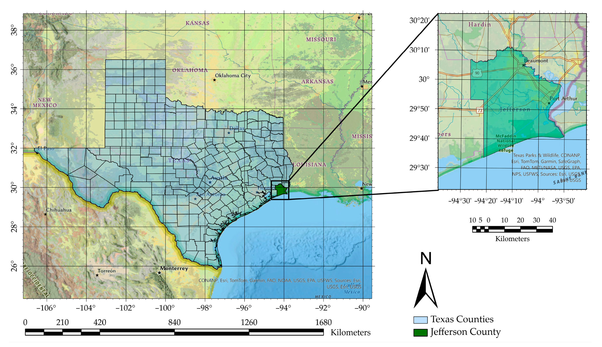
Figure 1. Location of the study area—Jefferson County, Texas, United States.
Remotesensing 17 03471 g001
Figure 6. Generating susceptibility maps using geospatial layers and Sentinel-1 SAR images.
Remotesensing 17 03471 g006
Figure 7. Three-dimensional architecture of a CNN model.
Remotesensing 17 03471 g007
Figure 8. Correlation matrix of features.
Remotesensing 17 03471 g008
Figure 9. AUC based on Flood Susceptibility derived from XGBoost, Random Forest, CNN, and Frequency Ratio.
Remotesensing 17 03471 g009
Figure 10. SHAP score graph for machine learning models.
Remotesensing 17 03471 g010
Figure 11. Flood Susceptibility maps of Jefferson County, Texas.
Remotesensing 17 03471 g011
Figure 12. Distribution of high-risk locations monitored by flood sensors across susceptibility classes as predicted by Random Forest, CNN, Frequency Ratio, and XGBoost models.
Remotesensing 17 03471 g012
Figure 13. Comparison of the ML model in the vicinity of SETX Regional Sensors: BM27 and BM12 (BM27 Location: 30.0423000, −94.1092000; BM12 Location: 30.0719000, −94.1303000).
Remotesensing 17 03471 g013
Figure 14. Comparison of XGBoost and BLE BLE_DEP0_2PCT in the vicinity of DHS sensors: BM27 and BM12 (BM27 Location: 30.0423000, −94.1092000; BM12 Location: 30.0719000, −94.1303000).
Remotesensing 17 03471 g014
Figure 15. Comparison of the XGBoost Model and the Local Community Task Force.
Remotesensing 17 03471 g015
Table 1. The table of acronyms.
AbbreviationDefinitionAbbreviationDefinition
AHPAnalytic Hierarchy ProcessMCDAMulti-Criteria Decision Analysis
ANNArtificial Neural NetworkNDVINormalized Difference Vegetation Index
AUCArea Under the CurveNHCNational Hurricane Center
BSABivariate Statistical AnalysisNLCDNational Land Cover Database
BLEBase Level EngineeringNRCSNatural Resources Conservation Service
BMBenchmark (sensor ID, e.g., BM27)NWSNational Weather Service
CNNConvolutional Neural NetworkPRISMParameter-elevation Regressions on Independent Slopes Model
DEMDigital Elevation ModelRFRandom Forest
DHSDepartment of Homeland SecurityROCReceiver Operating Characteristic
DOEDepartment of EnergyRSRemote Sensing
DTDecision TreeSARSynthetic Aperture Radar
ECDFEmpirical Cumulative Distribution FunctionSETxFCSSoutheast Texas Flood Coordination Study
FEMAFederal Emergency Management AgencySHAPShapley Additive Explanations
FNFalse NegativeSSURGOSoil Survey Geographic Database
FPFalse PositiveSVMSupport Vector Machine
FRFrequency RatioSWATSoil and Water Assessment Tool
FPRFalse Positive RateTNRISTexas Natural Resources Information System
GEEGoogle Earth EngineTNTrue Negative
GISGeographic Information SystemTPTrue Positive
LULCLand Use/Land CoverTPRTrue Positive Rate
LRLogistic RegressionTWITopographic Wetness Index
MLMachine LearningWoEWeights of Evidence
MLTMachine Learning TechniqueXGBoostExtreme Gradient Boosting
Table 2. The table of acronyms of the study.
FactorData TypesResolutionSource
DEMRaster30 m × 30 mUSGS Elevation DATA
SlopeRaster30 m × 30 mDEM
TWIRaster30 m × 30 mDEM
NDVIRaster30 m × 30 mLandsat 8 imagery
Soil typePolygon Soil Survey Geographic Database 2.3.2 [48]
Rock UnitePolygon RockUnitPoly250K, Texas (TNRIS) Geologic Data
LULCRaster30 m × 30 mNLCD 2021 Land Cover (CONUS)
Depression AreasRaster30 m × 30 mDEM
Soil Hydrology groupPolygon SSURGO Database
Average PrecipitationPolygon PRISM (2018–2023)
Distance for streams and waterbodiesPolygon Jefferson County Drainage District No. 6
Distance from RoadPolygon TxDOT Roadways dataset
Table 3. Number of flood cells based on flood occurrence.
Flood Occurrence (Times)123456
Number of water pixels496,973144,80635,63073421636238
Table 4. Frequency Ratio Calculations.
NameClassTotal AreaTotal Area PercentageNumber of Flood EventsEvent PercentageFrequency Ratio (Fr)FR × 100FR Weight
Dem<0.55543,13020.13211,81226.3391.308130.834130
0.55–1.42538,18919.94810,74923.9691.202120.153120
1.42–3.52538,87319.974831318.5370.92892.80592
3.52–7.12538,58619.963528011.7740.59058.97758
>7.12539,11519.983869219.3820.97096.99396
Slope<0.1903,00633.47123,41852.2191.560156.01156
0.1–1.61,111,19641.18813,14529.3110.71271.16671
>1.6683,69125.342828318.4700.72972.88372
Distance from the roads<120523,82519.416549712.2580.63163.13163
120–414554,92620.569630414.0570.68368.34168
414–921540,02420.017756416.8670.84384.26384
921–2247539,08419.98211,17124.9101.247124.663124
>2247540,03420.01714,31031.9091.594159.411159
Distance from Major Streams<100521,71819.33812,03226.8301.387138.740138
100–150181,8936.74230316.7591.002100.247100
150–200163,5466.06225755.7420.94794.71994
200–250149,1305.52822505.0170.90890.76590
>2501,681,60662.33024,95855.6530.89389.28789
Distance from minor Streams<25271,80410.07544049.8200.97597.47597
25–50198,5807.36132537.2540.98598.54898
50–75253,7179.40442589.4951.010100.962100
75–100191,0967.08332367.2161.019101.873101
>1001,782,69666.07729,69566.2151.002100.209100
TWI<4558,86720.715669514.9290.72172.06872
4–5.1510,61318.926570512.7210.67267.21567
5.1–7.5548,88920.345729016.2560.79979.89979
7.5–10.7532,72619.746977421.7951.104110.375110
>10.7546,79820.26815,38234.3001.692169.234169
NDVI<−0.135593,01821.98110,04522.3991.019101.902101
−0.13–0.21486,97718.050638914.2470.78978.92778
0.21–0.40543,43120.143781717.4310.86586.53686
0.40–0.53534,53919.81312,03526.8361.354135.44135
>0.53539,92820.013856019.0880.95495.37695
Soil TypeClay1,157,82542.91621,25747.4001.104110.44110
Clay loam292,74410.85140759.0870.83783.74183
Coarse sand33810.125390.0870.69469.39469
Fine sand33800.1251390.3102.474247.400247
Loam200,4637.43042659.5101.280127.99127
Sandy clay loam68,7692.54917593.9221.539153.87153
Silt loam76,4392.83315943.5541.255125.45125
Silty clay334,23512.38939058.7080.70370.28670
Silty clay loam98,6283.65620584.5891.255125.53125
Very fine sandy loam99340.368400.0890.24224.22324
water61,6292.2848111.8080.79279.16679
no-data390,46614.473490410.9350.75675.55675
Rock UnitF S27,5201.0203220.7180.70470.39070
Qal663,80124.604970521.6410.88087.95587
Qb647,10223.985995822.2050.92692.57692
Qbb79,9502.96322064.9191.660165.99165
Qbc1,134,38942.04720,19545.0321.071107.09107
Qbi44,2821.64112712.8341.727172.67172
Qd66890.248460.1030.41441.37141
Ql270.00100.0000.0000.0000
Wa94,1333.48911432.5490.73073.04773
LULCAgricultural Land1,052,06519.49818,37820.4901.051105.08105
Barren78900.2923280.7312.501250.09250
Developed457,82716.970457610.2040.60160.12960
Forested Upland36,6321.3584260.9500.70069.96069
Grassland and pasture13,7730.5115571.2422.433243.29243
Shrubland49880.185540.1200.65165.12865
Wetlands998,78237.02117,49339.0071.054105.36105
water125,9364.66830346.7651.449144.93144
Depression<01,348,0590.50029,0320.6471.296129.559129
>01,349,8340.50015,8140.3530.70570.47970
Average precipitation<1554535,49019.84810,05722.4261.130112.984112
1554–1602531,68719.707797817.7900.90390.26990
1602–1636549,57020.37011,09624.7421.215121.46121
1636–1695542,97220.12610,27422.9101.138113.83113
>1695538,17419.948544112.1330.60860.82160
Soil Hydrologic groupsA31,4591.1667411.6521.417141.701141
A/D17,3030.6411560.3480.54254.23854
B/D95,4113.53721994.9031.387138.65138
C19000.070130.0290.41241.16141
C/D78,1972.89815763.5141.212121.24121
D2,473,62391.68740,16189.5530.97797.67297
Table 5. Hyperparameters.
Random ForestXgboost
ParameterOptimum ValueParameterOptimum Value
n_estimators50lambda0.03251274199317688
max_depth20alpha0.6440814745700857
min_samples_split10colsample_bytree0.9
min_samples_leaf4subsample0.6
learning_rate0.008
n_estimators1000
max_depth60
min_child_weight1
Disclaimer/Publisher’s Note: The statements, opinions and data contained in all publications are solely those of the individual author(s) and contributor(s) and not of MDPI and/or the editor(s). MDPI and/or the editor(s) disclaim responsibility for any injury to people or property resulting from any ideas, methods, instructions or products referred to in the content.