Accurate Estimation of Forest Canopy Height Based on GEDI Transmitted Deconvolution Waveforms
Abstract
Highlights
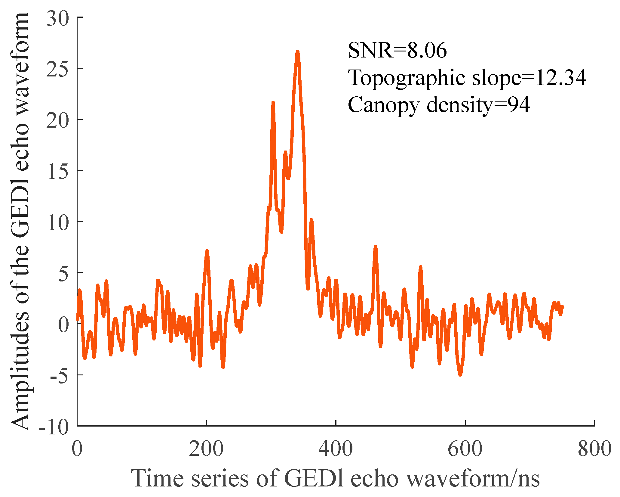
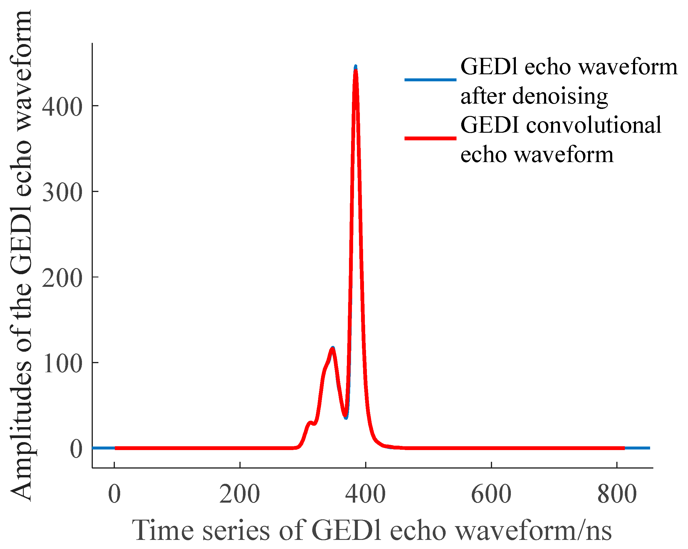
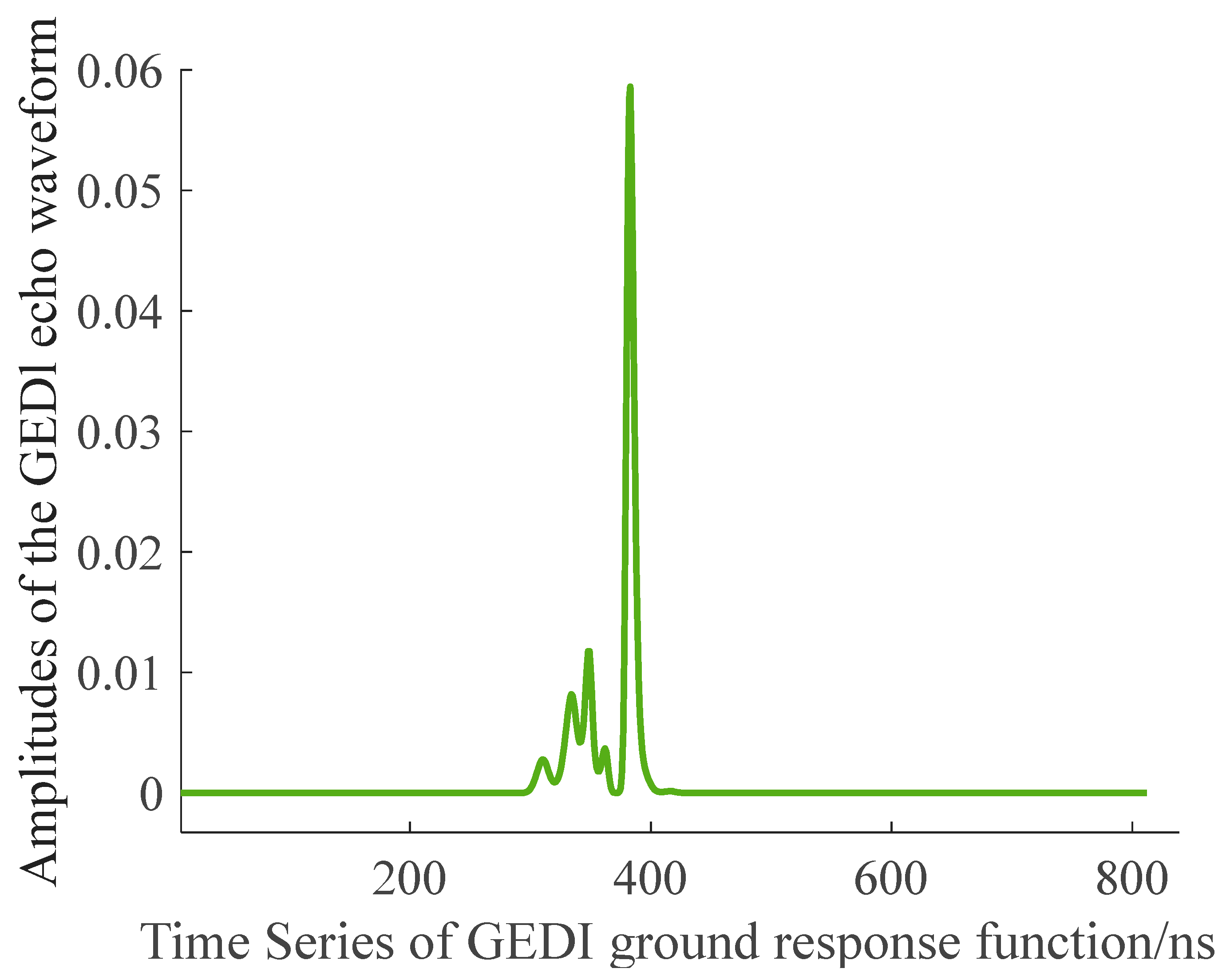
- The Inverse Deconvolution of Transmitted Waveforms (IDTW) algorithm effectively mitigates waveform broadening and overlap in GEDI data caused by the non zero half width of transmitted laser pulses (NHWTLP).
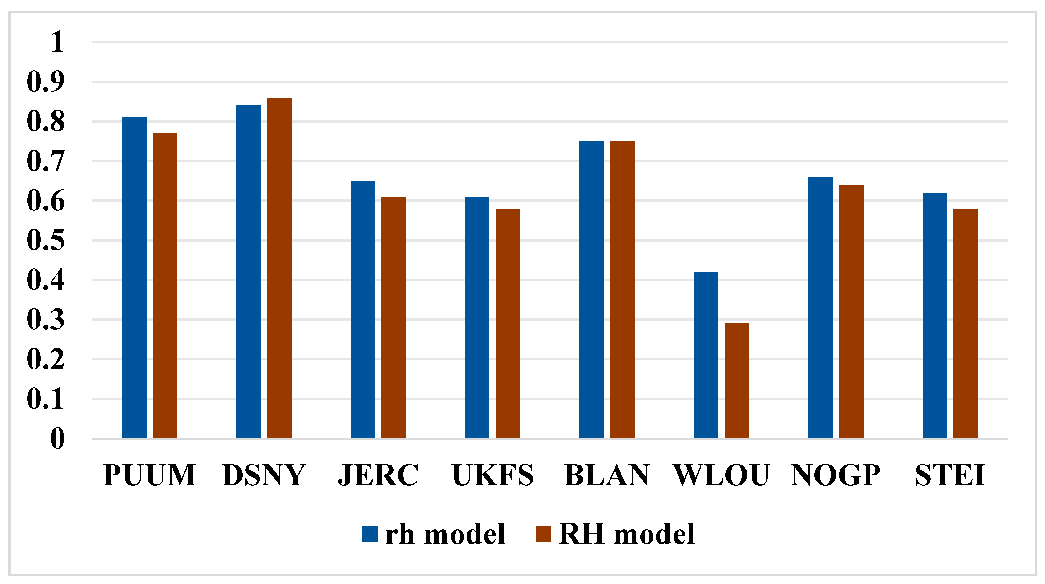
- The developed rh model outperforms the RH model across various conditions (beam types, terrain slopes, and canopy closures) in estimating forest canopy height(FCH).
- IDTW reduces dependence on LiDAR hardware pulse width precision while maintaining high canopy height accuracy, providing a cost effective solution for global forest structure monitoring.
- Combining IDTW with terrain slope constraints enables robust estimation of canopy height in complex terrain and high closure forests, supporting accurate assessment of forest carbon stocks and carbon cycle dynamics.
Abstract
1. Introduction
2. Materials
2.1. Study Area
2.2. GEDI Data
2.3. Airborne Data
2.4. Canopy Cover Data
3. Methods
3.1. Ground Response Function Construction via IDTW
3.1.1. IDTW Algorithm
3.1.2. Construction of the Ground Response Function
3.1.3. Optimization of Ground Response Function
3.2. Construction of FCH Estimation Model Combining the Ground Response Function and Slope Constraints
3.2.1. Extraction of Waveform Length Parameter
3.2.2. Construction of FCH Estimation Model
4. Results and Discussion
4.1. FCH Estimation Results for the GEDI Full-Power and Coverage Beams
4.2. FCH Estimation Under Different Terrain Slopes
4.3. FCH Estimation Under Different Canopy Covers
4.4. FCH Estimation Under Different Sites
5. Conclusions
- (1)
- The FCH estimation accuracy when using the rh model is higher than that with the RH model under conditions such as GEDI full-power beams and coverage beams, varying terrain slopes, different forest canopy densities, and different sites. This indicates that IDTW can effectively address the issues of waveform broadening and waveform overlap caused by NHWTLP.
- (2)
- The rh model, after the incorporation of terrain slope parameters, shows an improvement in FCH estimation accuracy under conditions such as GEDI full-power beams and coverage beams, varying terrain slopes, different forest canopy densities, and different sites. This indicates that the ground response function still contains terrain slope information, and the incorporation of terrain slope parameters into the rh model can reduce waveform broadening and overlap caused by non-flat terrain.
- (3)
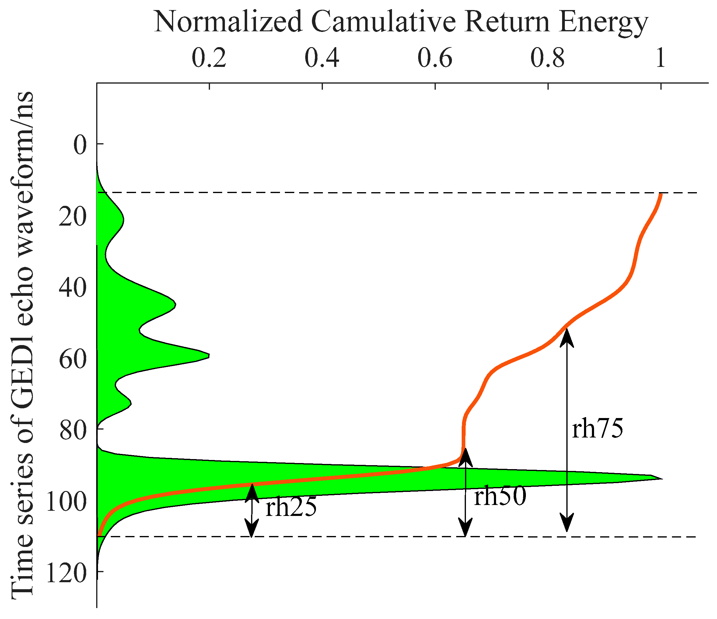
- The optimal parameter values of the rh model are lower than those of the RH model under conditions such as GEDI full-power beams and coverage beams, different terrain slopes, varying forest canopy densities, and different sites. The evidence indicates that IDTW can reduce the overlap of ground object information in the GEDI echo waveform, accurately reflecting the ground object projection area within the footprint. The findings also validate the applicability of the GEDI ground response function in FCH estimation from the perspective of the waveform energy distribution.
- (4)
- The rh model shows a greater improvement in the FCH estimation accuracy compared to the RH model for GEDI coverage beams, indicating that IDTW is more effective in denoising the echo waveforms of GEDI coverage beams than those of GEDI full-power beams.
Author Contributions
Funding
Data Availability Statement
Acknowledgments
Conflicts of Interest
Appendix A
| Symbol | Definition | Symbol | Definition | Symbol | Definition |
|---|---|---|---|---|---|
| Echo waveform | Horizontal projection area of the vegetation in the i-th layer in the vertical direction | Noise threshold | |||
| Transmitted waveform | Energy value of the transmitted waveform | Normalized waveform data of the denoised GEDI echo waveform | |||
| Ground response function | Standard deviation of the transmitted waveform, in ns | Normalized waveform data of the GEDI ground response function | |||
| GEDI noise-reduced transmitted waveform | Projected area of the ground object in the -th layer within the GEDI footprint | Background noise threshold | |||
| Raw GEDI transmitted waveform | Denoised GEDI echo waveform | Multiple of the standard deviation | |||
| GEDI echo waveforms after noise reduction | Number of iterations for Gaussian fitting of the GEDI echo waveform, which is set to 8 in this study | FCH estimation value | |||
| GEDI echo waveforms before noise reduction | Peak value of the Gaussian-fitted waveform | GEDI footprint diameter | |||
| Amplitude value of the m-th echo waveform | Frame number corresponding to the peak point of the Gaussian-fitted waveform | Terrain slope provided by the DTM product in the NEON data | |||
| Frame value corresponding to the peak point of the transmitted waveform | Standard deviation of the Gaussian-fitted waveform | Correlation coefficient values | |||
| Frame values of the echo waveform; the sum of these three amplitude values gives the total length of the echo waveform | GEDI ground response function obtained after n+1 iteration calculation | Vertical distance from the stop point of the GEDI echo waveform to the peak point of the ground wave | |||
| Total number of vertical layers of ground information within the footprint, divided at 0.15 m intervals | GEDI convolved echo obtained after the d-th iteration calculation | Tangent function | |||
| Amplitude value of the transmitted waveform in the i-th frame, in mJ | Difference function between the noise-reduced GEDI echo waveform and |
References
- Harris, N.L.; Gibbs, D.A.; Baccini, A.; Birdsey, R.A.; de Bruin, S.; Farina, M.; Fatoyinbo, L.; Hansen, M.C.; Herold, M.; Houghton, R.A. Global maps of twenty-first century forest carbon fluxes. Nat. Clim. Change 2021, 11, 234–240. [Google Scholar] [CrossRef]
- Li, X.; Li, L.; Ni, W.; Mu, X.; Wu, X.; Vaglio Laurin, G.; Vangi, E.; Stereńczak, K.; Chirici, G.; Yu, S. Validating GEDI tree canopy cover product across forest types using co-registered aerial LiDAR data. ISPRS J. Photogramm. Remote Sens. 2024, 207, 326–337. [Google Scholar] [CrossRef]
- Lai, J.; Kooijmans, L.M.J.; Sun, W.; Lombardozzi, D.; Campbell, J.E.; Gu, L.; Luo, Y.; Kuai, L.; Sun, Y. Terrestrial photosynthesis inferred from plant carbonyl sulfide uptake. Nature 2024, 634, 855–861. [Google Scholar] [CrossRef] [PubMed]
- Pan, Y.; Birdsey, R.A.; Fang, J.; Houghton, R.A.; Kauppi, P.E.; Kurz, W.A.; Phillips, O.L.; Shvidenko, A.Z.; Lewis, S.L.; Canadell, J.G.; et al. A large and persistent carbon sink in the world’s forests. Science 2011, 333, 988–993. [Google Scholar] [CrossRef]
- Han, Y.; Huang, J.; Ling, F.; Gao, X.; Cai, W.; Chi, H. RDNRnet: A reconstruction solution of NDVI based on SAR and optical images by residual-in-residual dense blocks. IEEE Trans. Geosci. Remote Sens. 2024, 62, 4402514. [Google Scholar] [CrossRef]
- Zhang, Q.; Zhou, H.; Ma, Y.; Wang, H.; Li, S.; Chen, Y. ICESat-2 derived canopy covers with radiometric and reflectance ratio corrections. IEEE Trans. Geosci. Remote Sens. 2024, 62, 4401714. [Google Scholar] [CrossRef]
- Tian, X.; Shan, J. ICESat-2 controlled integration of GEDI and SRTM data for large-scale digital elevation model generation. IEEE Trans. Geosci. Remote Sens. 2024, 62, 5703414. [Google Scholar] [CrossRef]
- Fareed, N.; Numata, I.; Cochrane, M.A.; Novoa, S.; Tenneson, K.; Flores de Melo, A.W.; Souza da Silva, S.; d’Oliveira, M.V.N.; Nicolau, A.; Zutta, B. Aboveground biomass modeling using simulated Global Ecosystem Dynamics Investigation (GEDI) waveform LiDAR and forest inventories in Amazonian rainforests. Forest Ecol. Manag. 2025, 578, 122491. [Google Scholar] [CrossRef]
- Adrah, E.; Jaafar, W.S.W.M.; Bajaj, S.; Yusoff, N.A.; Hashim, M. Analyzing canopy height variations in secondary tropical forests of Malaysia using NASA GEDI. IOP Conf. Ser. Earth Environ. Sci. 2021, 880, 012031. [Google Scholar] [CrossRef]
- Knapp, N.; Huth, A.; Fischer, R. Tree crowns cause border effects in area-based biomass estimations from remote sensing. Remote Sens. 2021, 13, 1592. [Google Scholar] [CrossRef]
- Cui, L.; Jiao, Z.; Zhao, K.; Sun, M.; Dong, Y.; Yin, S.; Zhang, X.; Guo, J.; Xie, R.; Zhu, Z.; et al. Retrieving forest canopy elements clumping index using ICESat GLAS lidar data. Remote Sens. 2021, 13, 948. [Google Scholar] [CrossRef]
- Chopping, M.; Wang, Z.; Schaaf, C.; Bull, M.A.; Duchesne, R.R. Forest aboveground biomass in the southwestern United States from a MISR multi-angle index, 2000–2015. Remote Sens. Environ. 2022, 275, 112964. [Google Scholar] [CrossRef]
- Rödig, E.; Knapp, N.; Fischer, R.; Bohn, F.J.; Dubayah, R.; Tang, H.; Huth, A. From small-scale forest structure to Amazon-wide carbon estimates. Nat. Commun. 2019, 10, 5088. [Google Scholar] [CrossRef] [PubMed]
- Lang, N.; Jetz, W.; Schindler, K.; Wegner, J.D. A high-resolution canopy height model of the Earth. Nat. Ecol. Evol. 2023, 7, 1778–1789. [Google Scholar] [CrossRef]
- Wang, B. Estimation of forest canopy height from spaceborne full-waveform LiDAR data using a bisection approximation decomposition method. Forests 2025, 16, 145. [Google Scholar] [CrossRef]
- Wang, S. Optimizing GEDI canopy height estimation and analyzing error impact factors under highly complex terrain and high-density vegetation conditions. Forests 2024, 15, 2024. [Google Scholar] [CrossRef]
- Duncanson, L.; Kellner, J.R.; Armston, J.; Dubayah, R.; Minor, D.M.; Hancock, S.; Healey, S.P.; Patterson, P.L.; Saarela, S.; Marselis, S.; et al. Aboveground biomass density models for NASA’s Global Ecosystem Dynamics Investigation (GEDI) LiDAR mission. Remote Sens. Environ. 2022, 270, 112845. [Google Scholar] [CrossRef]
- Hu, T.; Su, Y.; Xue, B.; Liu, J.; Zhao, X.; Fang, J.; Guo, Q. Mapping global forest aboveground biomass with spaceborne LiDAR, optical imagery, and forest inventory data. Remote Sens. 2016, 8, 565. [Google Scholar] [CrossRef]
- Duncanson, L.; Liang, M.; Leitold, V.; Armston, J.; Krishna Moorthy, S.M.; Dubayah, R.; Costedoat, S.; Enquist, B.J.; Fatoyinbo, L.; Goetz, S.J.; et al. The effectiveness of global protected areas for climate change mitigation. Nat. Commun. 2023, 14, 2908. [Google Scholar] [CrossRef]
- Zhang, W.; Xi, Y.; Brandt, M.; Ren, C.; Bai, J.; Ma, Q.; Fensholt, R. Stand structure of tropical forests is strongly associated with primary productivity. Commun. Earth Environ. 2024, 5, 796. [Google Scholar] [CrossRef]
- Rajabpour Rahmati, M.; Darvishsefat, A.A.; Baghdadi, N.; Namiranian, M.; Soofi Mariv, H. Estimation of forest canopy height in mountainous areas using ICESat-GLAS data. Iran. J. For. Poplar Res. 2015, 23, 90–103. [Google Scholar] [CrossRef]
- Jones, L.A.; Dean, C.D.; Mannion, P.D.; Farnsworth, A.; Allison, P.A. Spatial sampling heterogeneity limits the detectability of deep time latitudinal biodiversity gradients. Proc. R. Soc. B 2021, 288, 20202762. [Google Scholar] [CrossRef]
- Hofton, M.; Blair, J.B.; Story, S.; Yi, D. Algorithm Theoretical Basis Document (ATBD) for GEDI Transmit and Receive Waveform Processing for L1 and L2 Products; University of Maryland: College Park, MD, USA, 2019; Volume 44. [Google Scholar]
- Simard, M.; Pinto, N.; Fisher, J.B.; Baccini, A. Mapping forest canopy height globally with spaceborne LiDAR. J. Geophys. Res. Biogeosci. 2011, 116, 4021. [Google Scholar] [CrossRef]
- Iqbal, I.A.; Dash, J.; Ullah, S.; Ahmad, G. A novel approach to estimate canopy height using ICESat/GLAS data: A case study in the New Forest National Park, UK. Int. J. Appl. Earth Obs. Geoinform. 2013, 23, 109–118. [Google Scholar] [CrossRef]
- Wang, C.; Tang, F.X.; Li, L.W.; Li, G.C.; Cheng, F.; Xi, X.H. Wavelet analysis for ICESat/GLAS waveform decomposition and its application in average tree height estimation. IEEE Geosci. Remote Sens. Lett. 2013, 10, 115–119. [Google Scholar] [CrossRef]
- Lefsky, M.A.; Harding, D.J.; Keller, M.; Smith, A.M.S.; Hanan, N.P.; Healey, S.P. Estimates of forest canopy height and aboveground biomass using ICESat. Geophys. Res. Lett. 2005, 32, L15408. [Google Scholar] [CrossRef]
- Nie, S.; Wang, C.; Dong, P.; Li, Z.; Yuan, Y. A novel model for terrain slope estimation using ICESat/GLAS waveform data. IEEE Trans. Geosci. Remote Sens. 2017, 56, 217–227. [Google Scholar] [CrossRef]
- Hilbert, C.; Schmullius, C. Influence of surface topography on ICESat/GLAS forest height estimation and waveform shape. Remote Sens. 2012, 4, 2210–2235. [Google Scholar] [CrossRef]
- Wang, X.Y.; Huang, H.B.; Gong, P.; Liu, C.X.; Li, C.C.; Li, W.Y. Forest canopy height extraction in rugged areas with ICESat/GLAS data. IEEE Trans. Geosci. Remote Sens. 2014, 52, 4650–4657. [Google Scholar] [CrossRef]
- Hayashi, M.; Saigusa, N.; Oguma, H.; Yamagata, Y.; Takao, G. Quantitative assessment of the impact of typhoon disturbance on a Japanese forest using satellite laser altimetry. Remote Sens. Environ. 2015, 156, 216–225. [Google Scholar] [CrossRef]
- Xing, Y.; Gier, A.D.; Zhang, J.; Wang, L.H. An improved method for estimating forest canopy height using ICESat-GLAS full waveform data over sloping terrain: A case study in Changbai Mountains, China. Int. J. Appl. Earth Obs. Geoinform. 2010, 12, 385–392. [Google Scholar] [CrossRef]
- Corp, L.A.; Cook, B.D.; McCorkel, J.; Middleton, E.M. Data products of NASA Goddard’s LiDAR, hyperspectral, and thermal airborne imager (G-LiHT). In Proceedings of the Next-Generation Spectroscopic Technologies VIII, Baltimore, MD, USA, 20–24 April 2015; Volume 9482, p. 94821D. [Google Scholar] [CrossRef]
- Cook, B.D.; Corp, L.A.; Nelson, R.F.; Middleton, E.M.; Morton, D.C.; McCorkel, J.T.; Masek, J.G.; Ranson, K.J.; Ly, V.; Montesano, P.M. NASA Goddard’s LiDAR, Hyperspectral and Thermal (G-LiHT) Airborne Imager. Remote Sens. 2013, 5, 4045–4066. [Google Scholar] [CrossRef]
- Huang, J.; Xia, T. Multilevel adaptive photon cloud noise filtering algorithm for different observation time scenes in forest environments. IEEE Trans. Geosci. Remote Sens. 2023, 62, 5700816. [Google Scholar] [CrossRef]
- Zhang, X.; Liu, L.Y.; Wu, C.S.; Chen, X.D.; Gao, Y.; Xie, S.; Zhang, B. Development of a global 30 m impervious surface map using multisource and multitemporal remote sensing datasets with the Google Earth Engine Platform. Earth Syst. Sci. Data 2020, 12, 1625–1648. [Google Scholar] [CrossRef]
- Hancock, S.; Armston, J.; Hofton, M.; Sun, X.L.; Duncanson, L.I.; Tang, H.; Kellner, R.J.; Dubayah, R. The GEDI Simulator: A large-footprint waveform LiDAR simulator for calibration and validation of spaceborne missions. Earth Space Sci. 2019, 6, 294–310. [Google Scholar] [CrossRef]
- Wang, J.; Shen, X.; Cao, L. Upscaling forest canopy height estimation using waveform-calibrated GEDI spaceborne LiDAR and Sentinel-2 data. Remote Sens. 2024, 16, 2138. [Google Scholar] [CrossRef]
- Nie, S.; Wang, C.; Xi, X.H.; Li, G.Y.; Luo, S.Z.; Yang, X.B. Exploring the influence of various factors on slope estimation using large-footprint LiDAR data. IEEE Trans. Geosci. Remote Sens. 2018, 56, 6611–6621. [Google Scholar] [CrossRef]
- Fayad, I.; Baghdadi, N.; Alvares, C.A.; Stape, J.L.; Bailly, J.S.; Scolforo, H.F.; Cegatta, I.R.; Zribi, M.; Le Maire, G. Terrain slope effect on forest height and wood volume estimation from GEDI data. Remote Sens. 2021, 13, 2136. [Google Scholar] [CrossRef]
- Liu, C.; Wang, S. Estimating tree canopy height in densely forest-covered mountainous areas using GEDI spaceborne full-waveform data. ISPRS Ann. Photogramm. Remote Sens. Spatial Inf. Sci. 2022, V-1-2022, 25–32. [Google Scholar] [CrossRef]
- Folharini, S.; dos Santos, S.M.B.; Bento-Gonçalves, A.; Vieira, A. Estimation of tree height in burned areas with GEDI laser data in Northern Portugal and Galicia (Spain). Environ. Sci. Proc. 2022, 22, 50. [Google Scholar] [CrossRef]

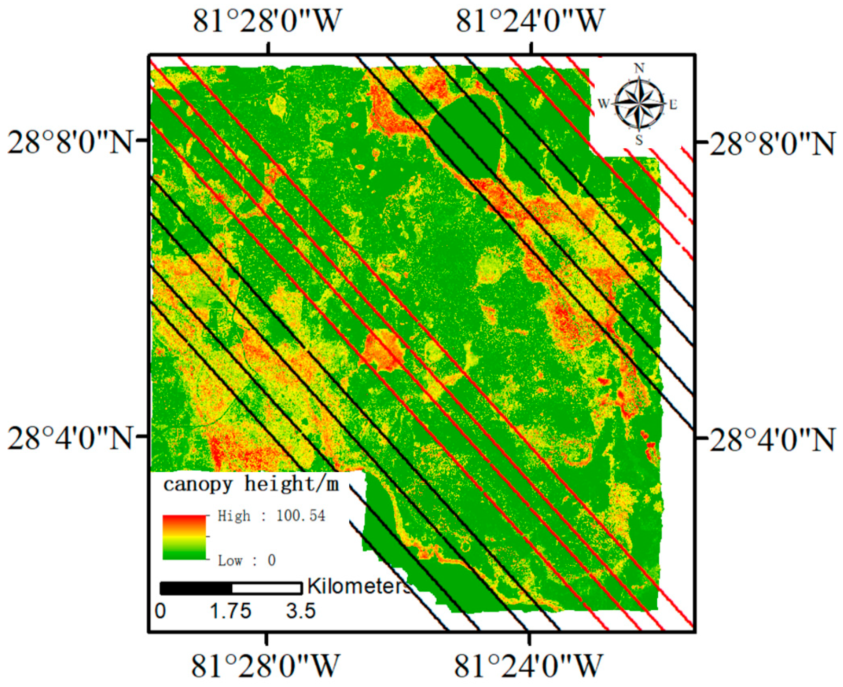
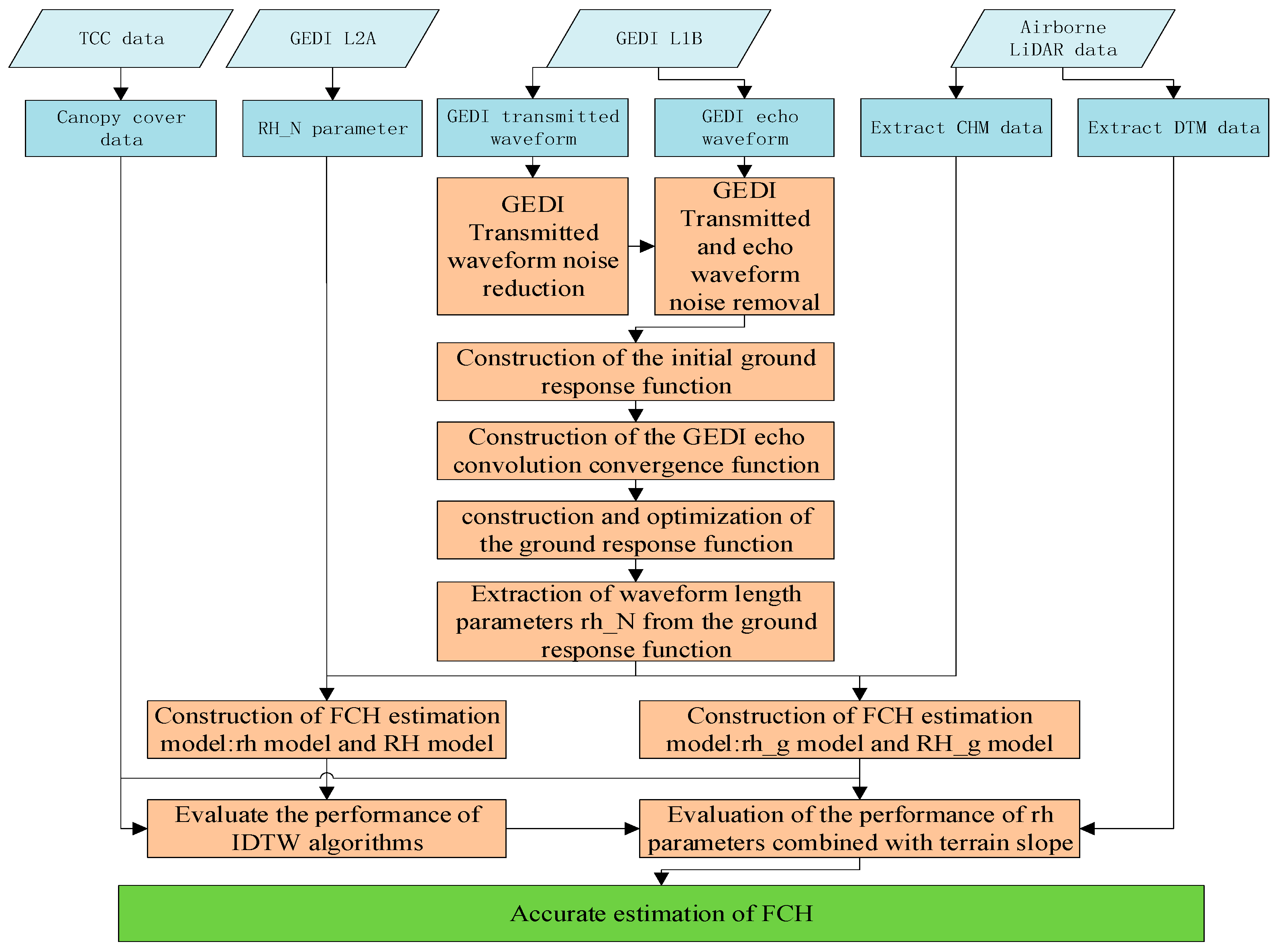


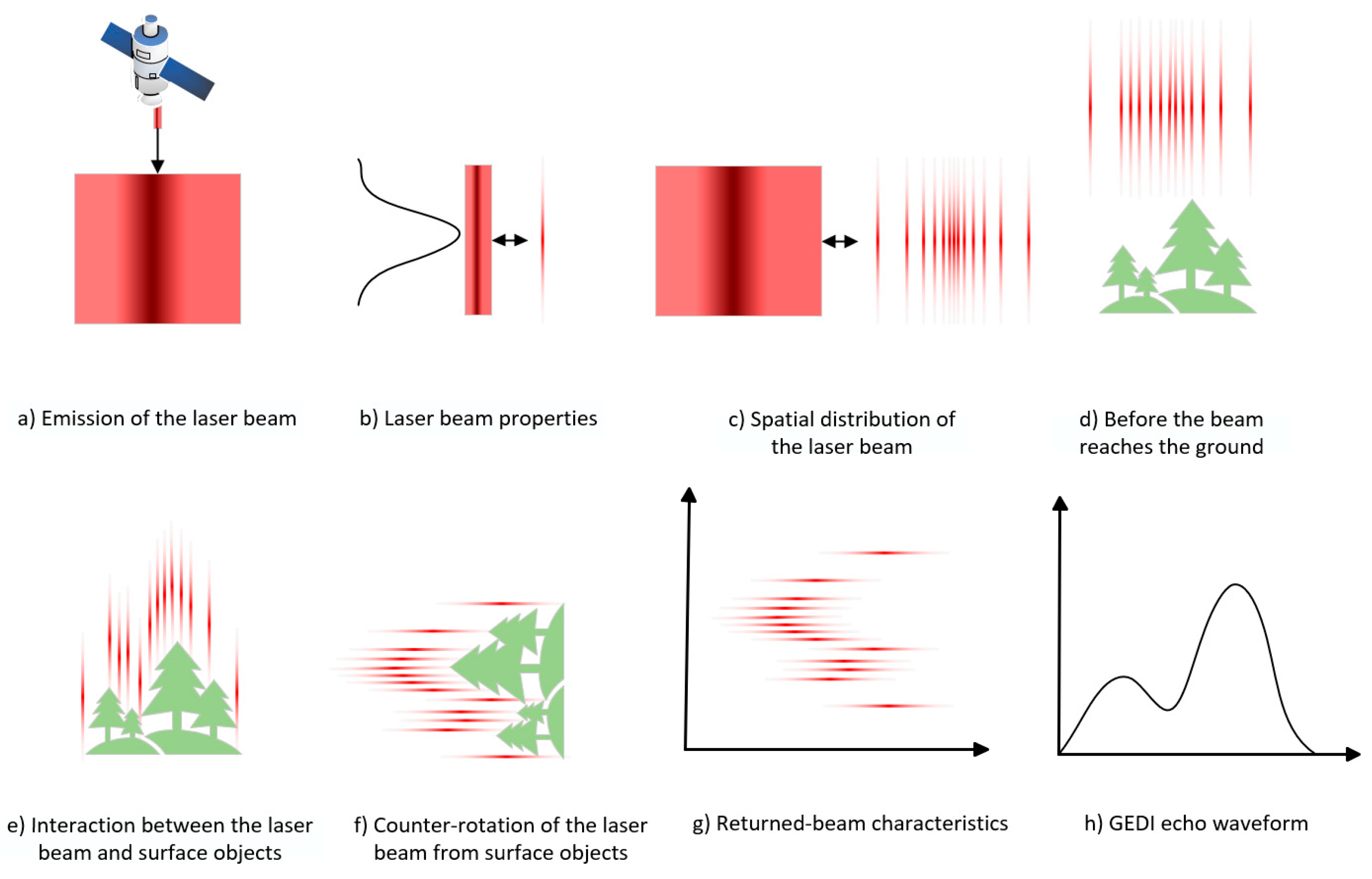
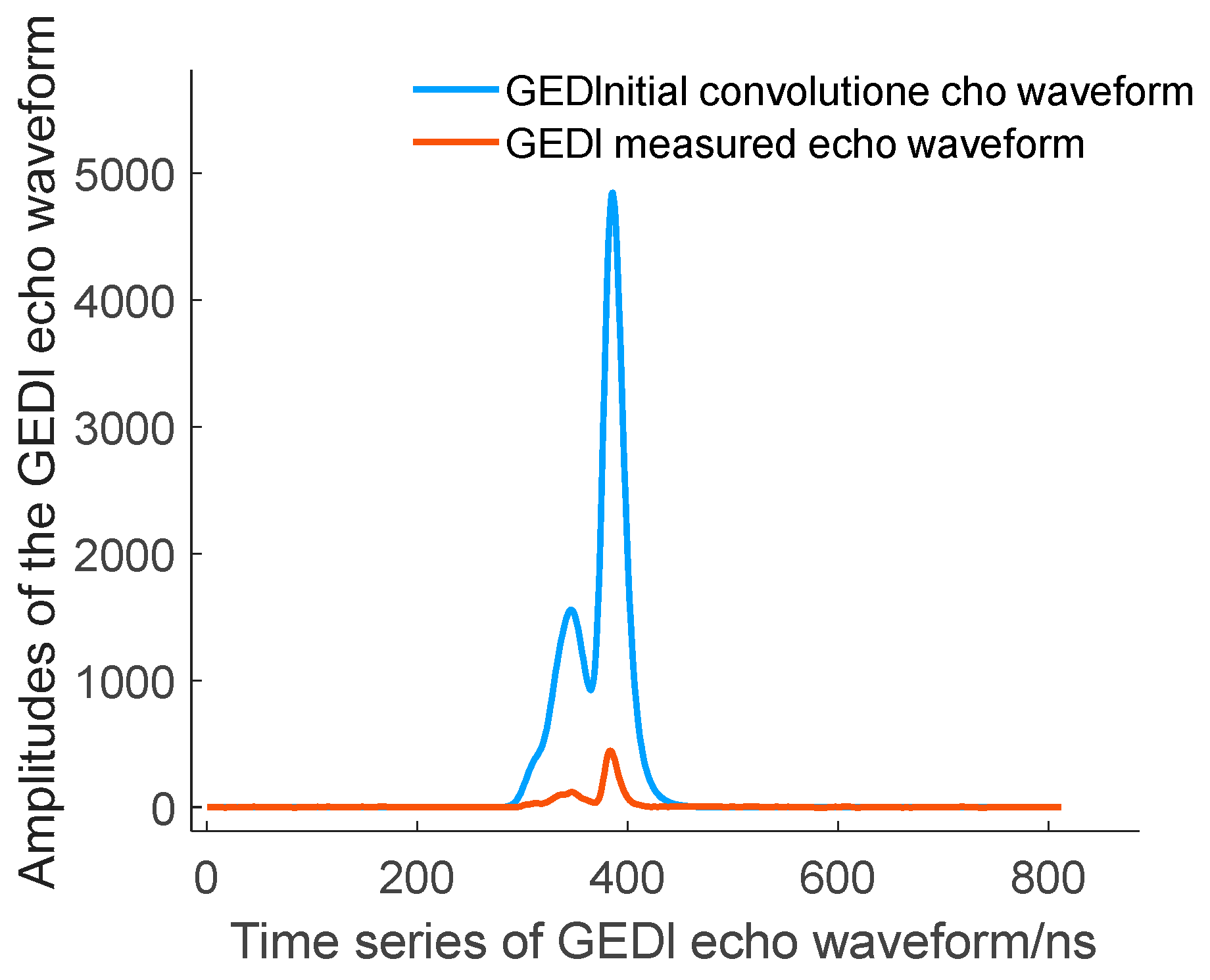

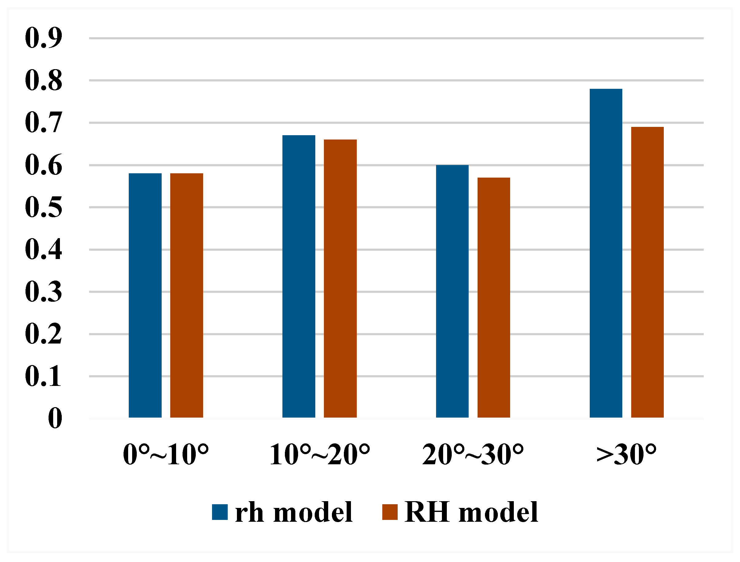
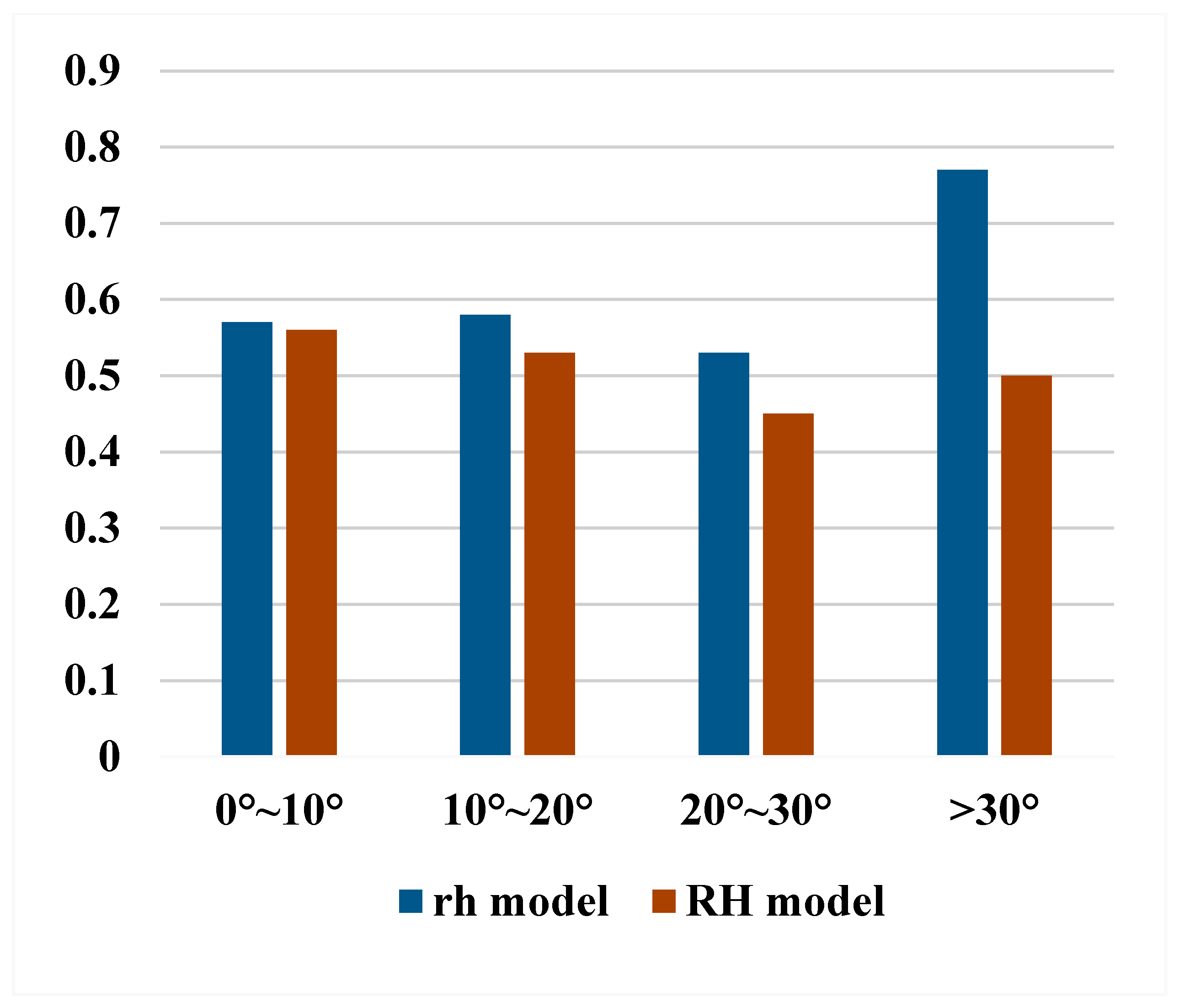
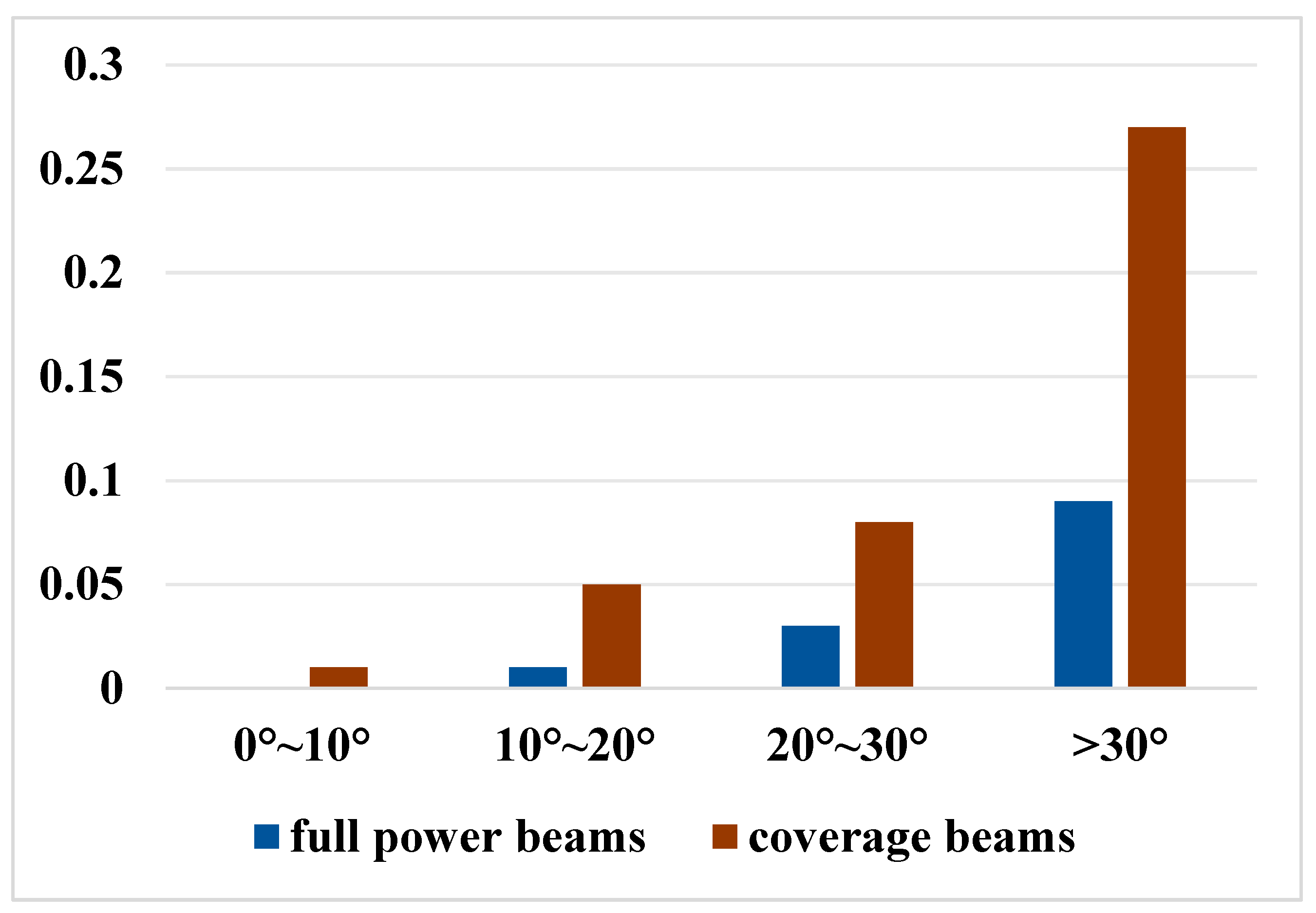
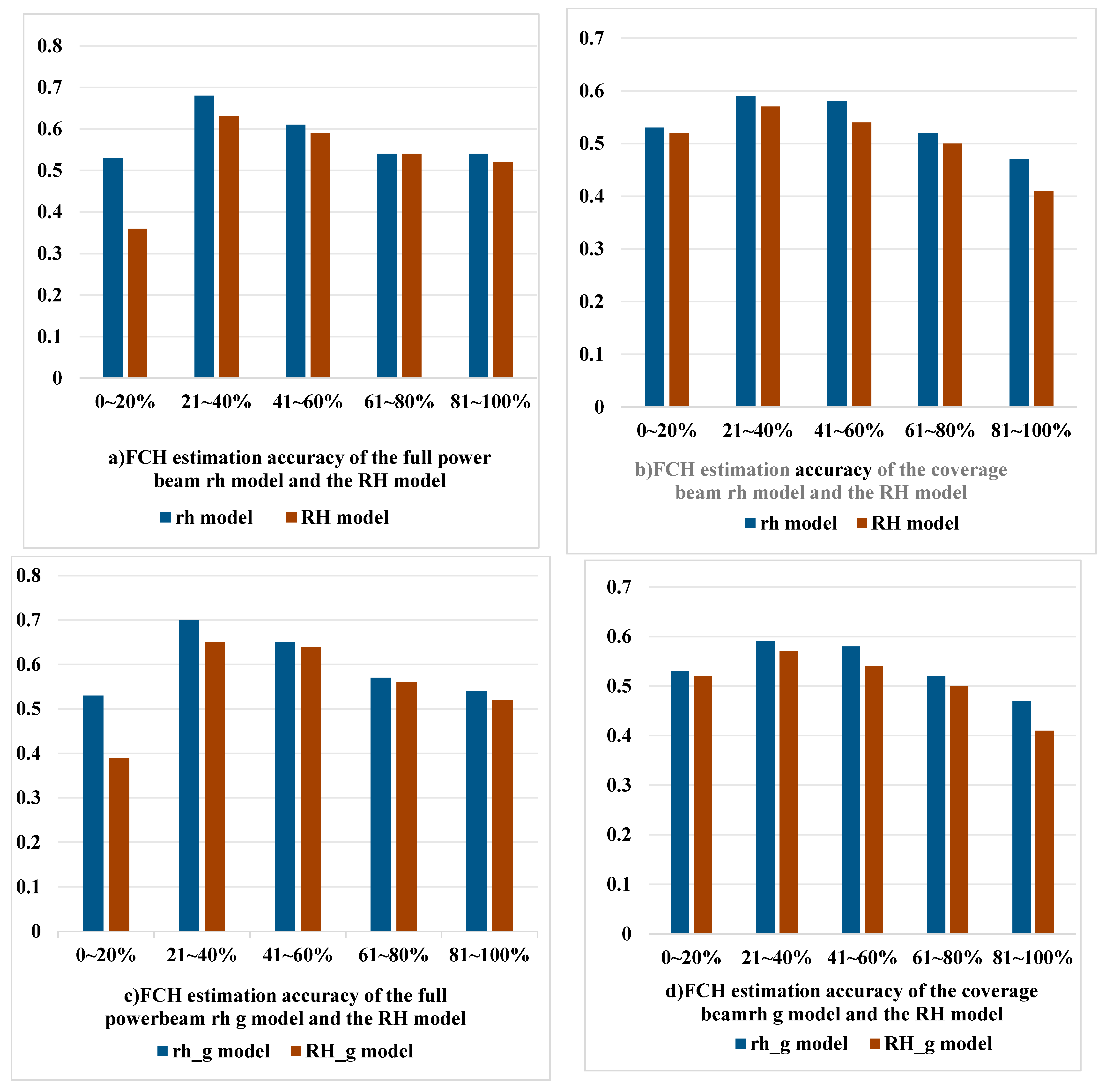
| Site Name | Longitude and Latitude Range | Acquisition Time | Number of Footprints | Tree Height Range | Terrain Slope Range | Canopy Density Range |
|---|---|---|---|---|---|---|
| PUUM | 19.48°N~19.63°N, 155.46°W~155.21°W | 1 Jan 2020 | 2411 | 0.00~26.91 | 0.22~40.42 | 0.00~100 |
| DSNY | 28.02°N~28.15°N, 81.50°W~81.36°W | 1 Sep 2021 | 2683 | 0.00~29.39 | 0.06~13.04 | 0.00~100 |
| JERC | 31.15°N~31.33°N, 84.58°W~84.35°W | 1 Sep 2021 | 5331 | 0.69~99.62 | 0.00~20.13 | 0.00~100 |
| UKFS | 38.94°N~39.10°N, 95.27°W~95.12°W | 1 Jul 2020 | 2078 | 0.00~27.21 | 0.02~35.88 | 0.00~100 |
| BLAN | 39.03°N~39.15°N, 78.11°W~77.93°W | 1 Aug 2021 | 6097 | 0.00~40.98 | 0.04~44.16 | 0.00~100 |
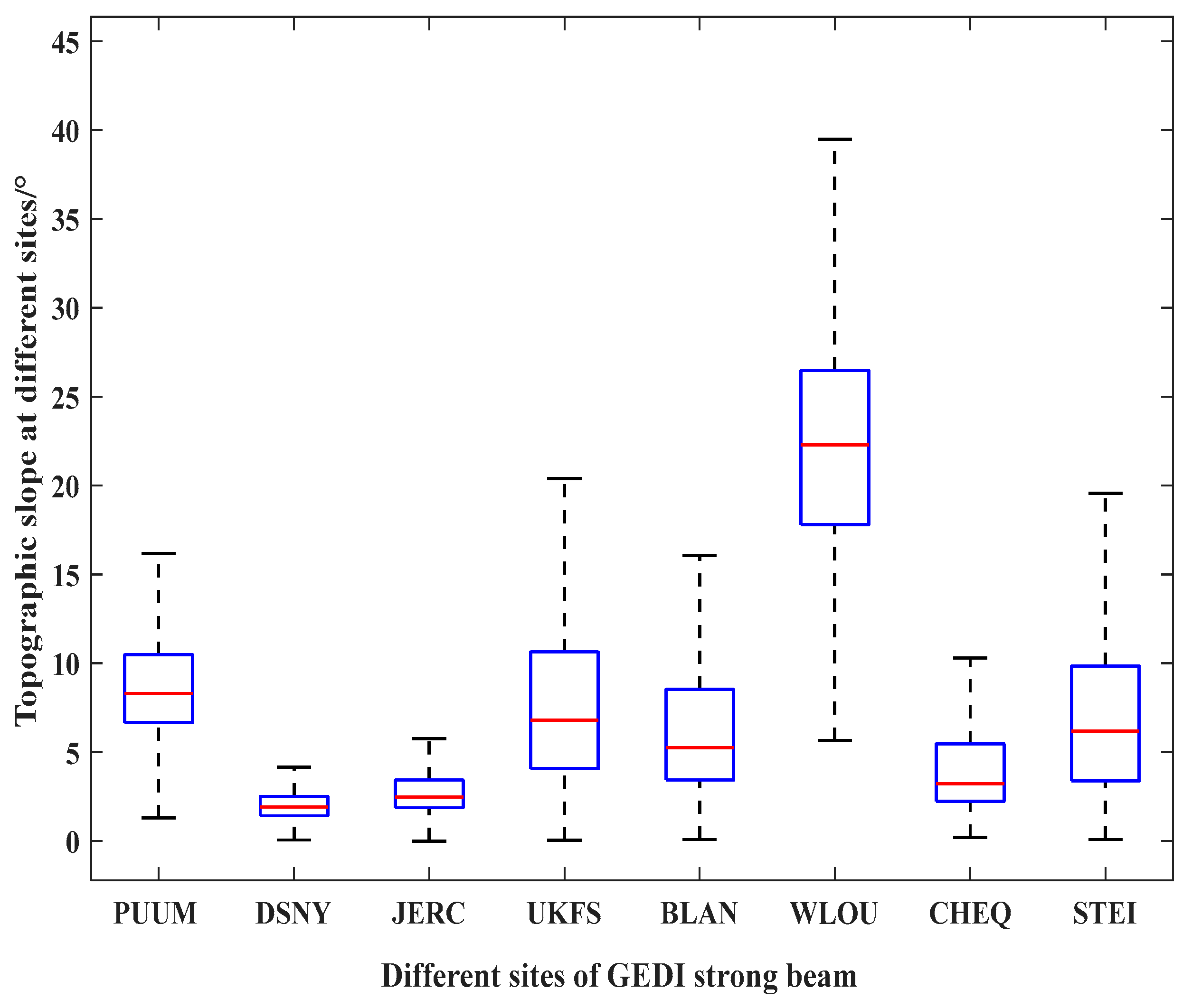
| WLOU | 39.86°N~39.91°N, 105.95°W~105.88°W | 1 Aug 2021 | 468 | 0.02~16.96 | 2.72~40.25 | 0.00~88 |
| NOGP | 45.76°N~45.85°N, 90.14°W~90.02°W | 1 Jun 2020 | 2277 | 0.00~27.35 | 0.09~20.65 | 0.00~100 |
| STEI | 45.43°N~45.57°N, 89.63°W~89.36°W | 1 Sep 2020 | 10,754 | 0.00~28.91 | 0.04~28.00 | 0.00~100 |
| Beam Name | Full-Power Beams | Coverage Beams | |
|---|---|---|---|
| Mean terrain slope/° | 6.09 | 6.26 | |
| Mean canopy cover/% | 57.00 | 63.59 | |
| Mean SNR | 22.83 | 18.56 | |
| Number of footprints | 18,288 | 13,811 | |
| model | optimum parameter | 96 | 92 |
| R2 | 0.58 | 0.57 | |
| RMSE | 5.23 | 4.58 | |
| _g model | optimum parameter | 96 | 92 |
| R2 | 0.61 | 0.58 | |
| RMSE | 5.21 | 4.55 | |
| model | optimum parameter | 98 | 95 |
| R2 | 0.58 | 0.56 | |
| RMSE | 5.54 | 4.72 | |
| model | optimum parameter | 98 | 95 |
| R2 | 0.60 | 0.56 | |
| RMSE | 5.45 | 4.71 | |
| Terrain Slope Range/° | 0~10 | 11~20 | 21~30 | >30 | |||||
|---|---|---|---|---|---|---|---|---|---|
| Beam Name | Full-Power Beams | Coverage Beams | Full-Power Beams | Coverage Beams | Full-Power Beams | Coverage Beams | Full-Power Beams | Coverage Beams | |
| Mean terrain slope/° | 4.28 | 4.33 | 13.37 | 13.33 | 23.53 | 23.19 | 33.68 | 32.86 | |
| Mean canopy cover/% | 53.36 | 59.99 | 73.90 | 79.15 | 79.50 | 78.66 | 77.51 | 66.41 | |
| Mean SNR | 22.83 | 18.82 | 23.01 | 17.53 | 22.81 | 16.30 | 20.95 | 15.23 | |
| Number of footprints | 15,162 | 11,192 | 2711 | 2323 | 366 | 274 | 49 | 22 | |
| model | optimum parameter | 97 | 92 | 95 | 93 | 89 | 91 | 46 | 52 |
| R2 | 0.58 | 0.57 | 0.67 | 0.58 | 0.60 | 0.53 | 0.78 | 0.77 | |
| RMSE | 5.66 | 4.59 | 4.24 | 4.56 | 4.78 | 5.31 | 3.96 | 3.51 | |
| _g model | optimum parameter | 97 | 92 | 95 | 93 | 89 | 91 | 60 | 52 |
| R2 | 0.59 | 0.58 | 0.67 | 0.58 | 0.61 | 0.55 | 0.81 | 0.77 | |
| RMSE | 5.61 | 4.55 | 4.24 | 4.56 | 4.72 | 5.17 | 3.71 | 3.50 | |
| model | optimum parameter | 98 | 95 | 96 | 95 | 90 | 58 | 45 | 40 |
| R2 | 0.58 | 0.56 | 0.66 | 0.53 | 0.57 | 0.45 | 0.69 | 0.50 | |
| RMSE | 5.67 | 4.64 | 4.30 | 4.81 | 4.94 | 5.70 | 4.73 | 5.19 | |
| model | optimum parameter | 98 | 95 | 96 | 95 | 90 | 58 | 85 | 40 |
| R2 | 0.59 | 0.57 | 0.66 | 0.54 | 0.59 | 0.48 | 0.75 | 0.50 | |
| RMSE | 5.62 | 4.59 | 4.30 | 4.81 | 4.82 | 5.54 | 4.26 | 5.19 | |
| Canopy Cover Range/° | 0~20 | 21~40 | 41~60 | 61~80 | 81~100 | ||||||
|---|---|---|---|---|---|---|---|---|---|---|---|
| Beam Name | Full-Power Beams | Coverage Beams | Full-Power Beams | Coverage Beams | Full-Power Beams | Coverage Beams | Full-Power Beams | Coverage Beams | Full-Power Beams | Coverage Beams | |
| Mean terrain slope/° | 4.67 | 4.58 | 5.46 | 5.22 | 4.98 | 5.11 | 5.98 | 6.35 | 7.35 | 7.27 | |
| Mean canopy cover/% | 1.33 | 1.44 | 29.15 | 29.04 | 49.47 | 49.21 | 70.37 | 70.72 | 95.52 | 95.93 | |
| Mean SNR | 23.27 | 19.00 | 23.17 | 17.93 | 22.87 | 17.60 | 22.84 | 17.64 | 22.48 | 17.55 | |
| Number of footprint points | 5476 | 3542 | 1003 | 557 | 1873 | 1070 | 1428 | 982 | 8508 | 7660 | |
| model | optimum parameter | 90 | 90 | 96 | 83 | 98 | 82 | 97 | 90 | 96 | 92 |
| R2 | 0.53 | 0.53 | 0.68 | 0.59 | 0.61 | 0.58 | 0.54 | 0.52 | 0.54 | 0.47 | |
| RMSE | 2.95 | 2.99 | 5.59 | 3.50 | 6.68 | 3.74 | 5.89 | 3.76 | 4.16 | 4.27 | |
| _g model | optimum parameter | 90 | 90 | 96 | 83 | 98 | 82 | 97 | 90 | 96 | 94 |
| R2 | 0.53 | 0.53 | 0.70 | 0.59 | 0.65 | 0.58 | 0.57 | 0.52 | 0.54 | 0.47 | |
| RMSE | 2.95 | 2.99 | 5.37 | 3.49 | 6.32 | 3.74 | 5.74 | 3.76 | 4.14 | 4.26 | |
| model | optimum parameter | 98 | 93 | 98 | 87 | 98 | 85 | 99 | 93 | 97 | 95 |
| R2 | 0.36 | 0.52 | 0.63 | 0.57 | 0.59 | 0.54 | 0.54 | 0.50 | 0.52 | 0.41 | |
| RMSE | 5.99 | 3.01 | 6.03 | 3.59 | 6.84 | 3.92 | 5.93 | 3.85 | 4.25 | 4.49 | |
| model | optimum parameter | 98 | 93 | 98 | 86 | 98 | 85 | 99 | 93 | 97 | 95 |
| R2 | 0.39 | 0.52 | 0.65 | 0.58 | 0.64 | 0.54 | 0.56 | 0.50 | 0.52 | 0.41 | |
| RMSE | 5.84 | 3.01 | 5.80 | 3.57 | 6.47 | 3.91 | 5.76 | 3.84 | 4.24 | 4.49 | |
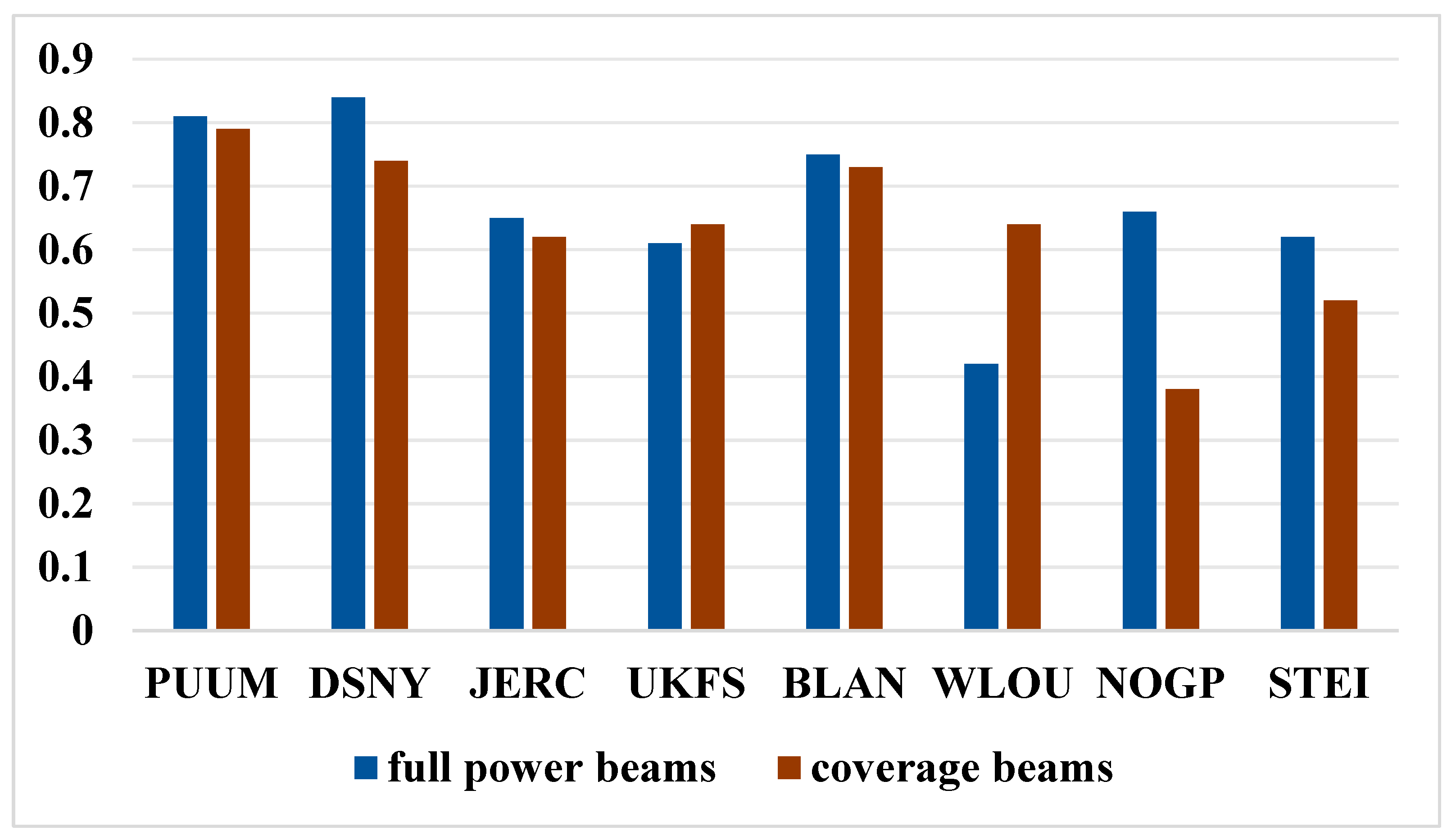
| Site Name | PUUM | DSNY | JERC | UKFS | BLAN | WLOU | NOGP | STEI | |
|---|---|---|---|---|---|---|---|---|---|
| Mean terrain slope/° | 8.83 | 2.14 | 2.96 | 7.82 | 7.10 | 22.27 | 4.28 | 7.21 | |
| Mean canopy cover/% | 64.33 | 45.63 | 31.71 | 35.30 | 43.97 | 49.55 | 86.39 | 83.88 | |
| Mean SNR | 21.23 | 23.69 | 22.34 | 21.04 | 22.56 | 23.77 | 21.33 | 22.72 | |
| Number of footprint points | 1891 | 1748 | 3338 | 1314 | 3675 | 181 | 1215 | 4926 | |
| model | optimum parameter | 86 | 82 | 98 | 97 | 93 | 87 | 52 | 95 |
| R2 | 0.81 | 0.84 | 0.65 | 0.61 | 0.75 | 0.42 | 0.66 | 0.62 | |
| RMSE | 2.43 | 2.52 | 6.09 | 4.01 | 4.50 | 2.42 | 3.54 | 3.66 | |
| _g model | optimum parameter | 86 | 82 | 98 | 97 | 93 | 87 | 52 | 95 |
| R2 | 0.81 | 0.85 | 0.65 | 0.62 | 0.76 | 0.51 | 0.66 | 0.62 | |
| RMSE | 2.39 | 2.49 | 6.08 | 3.98 | 4.44 | 2.24 | 3.53 | 3.66 | |
| model | optimum parameter | 93 | 84 | 100 | 100 | 96 | 94 | 59 | 98 |
| R2 | 0.77 | 0.86 | 0.61 | 0.58 | 0.75 | 0.29 | 0.64 | 0.58 | |
| RMSE | 2.65 | 2.42 | 100 | 4.19 | 4.57 | 2.69 | 3.62 | 3.85 | |
| model | optimum parameter | 93 | 84 | 100 | 100 | 96 | 94 | 59 | 98 |
| R2 | 0.77 | 0.86 | 0.61 | 0.59 | 0.75 | 0.40 | 0.64 | 0.58 | |
| RMSE | 2.63 | 2.39 | 6.40 | 4.11 | 4.54 | 2.24 | 3.62 | 3.85 | |
| Site Name | PUUM | DSNY | JERC | UKFS | BLAN | WLOU | NOGP | STEI | |
|---|---|---|---|---|---|---|---|---|---|
| Mean terrain slope/° | 9.13 | 2.14 | 2.73 | 7.31 | 7.40 | 17.91 | 3.91 | 7.12 | |
| Mean canopy cover/% | 79.62 | 37.48 | 27.93 | 30.36 | 51.89 | 61.55 | 93.27 | 82.46 | |
| Mean SNR | 16.50 | 17.91 | 16.41 | 18.83 | 17.79 | 16.06 | 19.66 | 17.93 | |
| Number of footprint points | 520 | 935 | 1993 | 764 | 2422 | 287 | 1062 | 5828 | |
| model | optimum parameter | 94 | 77 | 91 | 93 | 91 | 77 | 41 | 95 |
| R2 | 0.79 | 0.74 | 0.62 | 0.64 | 0.73 | 0.64 | 0.38 | 0.52 | |
| RMSE | 2.34 | 2.55 | 5.79 | 3.74 | 4.78 | 2.21 | 4.25 | 4.12 | |
| _g model | optimum parameter | 93 | 77 | 91 | 93 | 91 | 77 | 41 | 95 |
| R2 | 0.79 | 0.74 | 0.62 | 0.65 | 0.73 | 0.67 | 0.42 | 0.52 | |
| RMSE | 2.33 | 2.54 | 5.78 | 3.72 | 4.74 | 2.12 | 4.16 | 4.12 | |
| model | optimum parameter | 100 | 85 | 100 | 100 | 91 | 92 | 40 | 98 |
| R2 | 0.74 | 0.73 | 0.53 | 0.58 | 0.73 | 0.54 | 0.34 | 0.45 | |
| RMSE | 2.61 | 2.58 | 6.45 | 4.07 | 4.79 | 2.50 | 4.41 | 4.44 | |
| model | optimum parameter | 100 | 85 | 100 | 100 | 91 | 85 | 40 | 98 |
| R2 | 0.74 | 0.73 | 0.53 | 0.58 | 0.73 | 0.59 | 0.36 | 0.45 | |
| RMSE | 2.61 | 2.56 | 6.45 | 4.05 | 4.76 | 2.35 | 4.34 | 4.43 | |
Disclaimer/Publisher’s Note: The statements, opinions and data contained in all publications are solely those of the individual author(s) and contributor(s) and not of MDPI and/or the editor(s). MDPI and/or the editor(s) disclaim responsibility for any injury to people or property resulting from any ideas, methods, instructions or products referred to in the content. |
© 2025 by the authors. Licensee MDPI, Basel, Switzerland. This article is an open access article distributed under the terms and conditions of the Creative Commons Attribution (CC BY) license (https://creativecommons.org/licenses/by/4.0/).
Share and Cite
Cai, L.; Wu, J.; Somsack, I.; Zhao, X.; He, J. Accurate Estimation of Forest Canopy Height Based on GEDI Transmitted Deconvolution Waveforms. Remote Sens. 2025, 17, 3412. https://doi.org/10.3390/rs17203412
Cai L, Wu J, Somsack I, Zhao X, He J. Accurate Estimation of Forest Canopy Height Based on GEDI Transmitted Deconvolution Waveforms. Remote Sensing. 2025; 17(20):3412. https://doi.org/10.3390/rs17203412
Chicago/Turabian StyleCai, Longtao, Jun Wu, Inthasone Somsack, Xuemei Zhao, and Jiasheng He. 2025. "Accurate Estimation of Forest Canopy Height Based on GEDI Transmitted Deconvolution Waveforms" Remote Sensing 17, no. 20: 3412. https://doi.org/10.3390/rs17203412
APA StyleCai, L., Wu, J., Somsack, I., Zhao, X., & He, J. (2025). Accurate Estimation of Forest Canopy Height Based on GEDI Transmitted Deconvolution Waveforms. Remote Sensing, 17(20), 3412. https://doi.org/10.3390/rs17203412


